Abstract

In this paper, we study a Deep Reinforcement Learning (DRL) based framework for an online end-user service provisioning in a Network Function Virtualization (NFV)-enabled network. We formulate an optimization problem aiming to minimize the cost of network resource utilization. The main challenge is provisioning the online service requests by fulfilling their Quality of Service (QoS) under limited resource availability. Moreover, fulfilling the stochastic service requests in a large network is another challenge that is evaluated in this paper. To solve the formulated optimization problem in an efficient and intelligent manner, we propose a Deep Q-Network for Adaptive Resource allocation (DQN-AR) in NFV-enable network for function placement and dynamic routing which considers the available network resources as DQN states. Moreover, the service’s characteristics, including the service life time and number of the arrival requests, are modeled by the Uniform and Exponential distribution, respectively. In addition, we evaluate the computational complexity of the proposed method. Numerical results carried out for different ranges of parameters reveal the effectiveness of our framework. In specific, the obtained results show that the average number of admitted requests of the network increases by 7 up to 14$\%$ and the network utilization cost decreases by 5 and 20$\%$.
Index Terms— Deep reinforcement learning, service lifetime, resource allocation, NFV.

Online Service Provisioning in NFV-enabled Networks Using Deep Reinforcement Learning Ali Nouruzi, Abolfazl Zakeri, , Mohamad Reza Javan, , Nader Mokari, , Rasheed Hussain, , Ahsan Syed Kazmi, A. Nouruzi, A. Zakeri and N. Mokari are with the Department of Electrical and Computer Engineering, Tarbiat Modares University, Tehran, Iran, (e-mail: nader.mokari@modares.ac.ir). M. R. Javan is with the Department of Electrical Engineering, Shahrood University of Technology, Iran, (e-mail: javan@shahroodut.ac.ir). R. Hussain and A. S. Kazmi are with the Institute of Information Security and Cyber-Physical Systems, Innopolis University, Russia, (e-mail: r.hussain@innopolis.ru).

I INTRODUCTION

I-A State of The Art and Motivation

In recent years, new applications have emerged rapidly with diverse Quality of Service (QoS) requirements [1]. To meet their requirements in an efficient manner with a common physical infrastructure, exploiting advanced technologies is indispensable where these technologies are expected to have pivotal impacts on network performance in terms of enhancing QoS and resource efficiency which result in cost reduction. One such technology is Network Function Virtualization (NFV) providing an array of benefits such as great flexibility, resource efficiency, and cost reduction [2]. However, in such an NFV-enabled network, providing an efficient resource allocation algorithm is a challenging task. In addition, handle online service requests and also service arrival and departure and its effect on the network resources are the other challenges that we have in this paper. To tackle these challenges and design adaptive and intelligent networks, recently, Deep Reinforcement Learning (DRL) based methods have been used to solve various resource allocation problems[3, 4].
Besides, devising online and adaptive/on-demand service provisioning algorithms under dynamic network resource variations is another challenging task in NFV-enabled networks. Online and on-demand services by considering lifetime, i.e, while previously provisioned services are running, new service requests can arrive. Recently, some researchers have made great efforts to address the mentioned challenges, but, to the best of our knowledge, a few researchers consider the lifetime and online service requests, and the effect of this, on the Resource Allocation (RA) problem [5, 6, 7]. The prevailing works inspire us to seek a “smart“ and “online” service provisioning method with considering service “lifetime” in a NFV-enabled network. The term “service” indicates a type of end user request with specific QoS and Service Function Chain (SFC) characteristics, and “provisioning” means that such request’s requirements are fulfilled, hence, the service request is admitted. In brief, this work focuses on a main question which is: how a service provider offers heterogeneous services with a probabilistic lifetime on the common physical resources in a smart and efficient manner?

I-B Research Outputs and Contributions

Different from previous works [8, 7, 9], this work provides a DRL-based online service provisioning algorithm in an NFV-enabled network in which the considered service requests are online with a probabilistic lifetime. In addition, by deploying the proposed online service provisioning method, new requests can be served while previously accepted services are running.
The main results and contributions of this work are listed as follows:
$\bullet$ We propose a new service assurance model leveraging NFV to perform their Network Functions (NFs) and guarantee QoS in terms of latency and bandwidth. To this end, we formulate an optimization problem with constraints on the QoS and the limitation of network resources.
$\bullet$  We deploy DRL method to fulfill the different requests at each time under dynamic network resources in a long-term run. To improve the convergence speed of the considered case with large number of states and large action space, we deploy a Deep Q-Network (DQN) algorithm.
$\bullet$ We propose an online service provisioning method in which each user has a service timeline and new users can request service at each time slot while some services are running from the previous time slots. We also consider the dynamics of resource consumption and release in the network due to admitting new services and terminating previous services. Moreover, request arrivals are modeled by Uniform distribution, and service duration time (service time) is modeled by the exponential distribution.
$\bullet$ To apply the DQN algorithm for RA (i.e., solving the optimization problem), we develop the available calculation algorithm that updates the state space (e.g., due to resource releasing or failure occurring) at the beginning of each time slot to find an appropriate action.
$\bullet$ To evaluate the performance of the proposed method, we consider different baselines. The obtained results unveil that the proposed method has considerable performance. The main baselines are greedy and online-Tabu search algorithms which are well known methods in online algorithm consideration.

I-C Related Work

Recently some works define a service with a specific SFC which includes a set of Virtual Network Functions (VNFs) and these VNFs need to be executed in a tolerable delay [10], [11]. These VNFs run on a specific virtual machines which are created on top of the physical network by leveraging NFV. Hereupon, service provisioning means that the requested SFC with QoS requirement for each request is done successfully by performing the SFC and RA in the NFV environment [12]. The basic principles of NFV Resource Allocation (NFV-RA) is studied in [5] comprehensively. Also, online scheduling with minimizing the total execution time of VNFs is studied in [13]. Furthermore, the authors in [6] propose NFV-RA for traffic routing by deploying game theory. They focus on routing and embedding of VNFs and do not consider the scheduling problem. Similarly, placement of VNF instances for different services with link allocation and fixed delay for links is studied in [14]. Delay-aware cost minimization for random arrival service requests by deploying stochastic dual gradient method is studied in [15].

At the same time, DRL-based methods to solve various RA problems have attracted much attention [16, 17, 18]. In [19], a ML algorithm for extracting feature of data traffic in NFV-cloud network for predicting computation and demands of resources is deployed. In [20], DRL based mechanism with Markov Decision Process (MDP) is proposed for reducing congestion probability and also choosing transmission path for routing and traffic engineering. Network congestion probability reduce to $50\%$ with compare to Open Short First Path (OSFP) routing method. Because routing and function placement problems are related to each other, [21] proposes a function placement and chaining schemes, jointly with Binary Integer Programming (BIP) for minimizing End to End (E2E) delay, and then use Restricted Boltzmann Machine (RBM) output to determine the next hope node in the network. The authors in [22] proposes multi-task deep learning for routing and dynamic SFC with considering network status for predicting the routing path. Lastly, in [23], the authors use Integer Linear Programming (ILP) and multi layer perceptron to minimize E2E delay and placement of VNFs. In [24], the authors propose multi-objective programming and assume that access points work as a player in a game theory based problem that minimizes OpEx and average response time. In [25],the authors study providing IoT services in an NFV-enabled network by deploying DRL. Aiming to minimize the processing and transition delay, the proposed DRL method reduces the total delay to around $200$ms that has decreased up to 3 times compared to other baselines. In [26], the anthers propose a matching-based scheduling method that reduces the scheduling time in a NFV-enabled network up to $50\%$ compared to the Round-Robin scheduling method. Aiming to provide a cost-efficient dynamic resource management in a NFV-enabled network, the authors in [27] propose a practical method that reduces CPU utilization up to $10\%$ compared to the traditional approaches. In addition, the authors in [28, 29, 30] study the performance of the DRL-based methods for RA in the context of a NFV-enabled network where th obtained results show a significant improvement in the results obtained results compared to the traditional optimization methods. Motivated by significant effectiveness of DRL-based algorithm for RA in NFV-enabled networks, we propose a DRL-based algorithm for service provision in an NFV-enabled network. In addition, concerning the ability of DRL to support online algorithms, the proposed DQN algorithm is adopted an online RA algorithm that different from previous works [31, 32, 33], we assume that the services arrive based on the real stochastic model. Moreover, the required resources are allocated to the services while the subsequent services arrive. We summarize related works and compare them with our work in Table. I.

Table I: Related Works Summary

Ref.	Scenarios	Strategy	Main Contribution	Differences with this work
[20]	Routing and traffic engineering	Using DQN for Routing algorithm	Proposing an online routing for Routing algorithm	Considering nodes with several VMs and services specification
[25]	NFV (SFC & Routing)	SFC embedding for NFV-enabled IoT and routing by shortest path algorithm	Dynamic SFC embedding	Dynamic routing algorithm by considering links state
[26]	NFV (SFC & Scheduling)	Matching-Based VNF Scheduling	RA to VNF over time with a matching scheme	Online service assurance with considering VM and links and using DQN
[22]	NFV (SFC & Routing)	Multi task Deep learning	Learning traffic routing by SFC information	Objective, function placement with considering VM states and dynamic routing algorithm by considering links state
[21]	NFV (SFC & Routing)	Applying Deep learning (RBM) to solve a BIP	Minimizing E2E delay with considering SFC path	Objective, VM state function placement consideration and link’s state dynamic routing
[27]	NFV (SFC)	Deploying testbed	Real-time flow monitoring and dynamic resource management	Real service consideration and evaluation of service life time
[28]	NFV (SFC & Routing)	Deploying DRL to solve MILP for optimize resource utilization	Near optimal results is obtained	Evaluation of effect of network topology and geo-distributed DC
[7]	NFV (SFC)	Deploying DRL to function placement	Deploying DRL for SFC	Dynamic routing and considering real service characteristics
[29]	NFV (SFC & Routing)	Deploying DRL for solving BIP	Dynamic SFC embedding	Objective and node by node dynamic routing
[30]	NFV (SDN & Routing)	Deploying DRL to solve mixed integer quadratic constrained (MIQCP) programming	Real time traffic model and NF migration	Objective and service life time consideration and evaluation of network topology

I-D Paper Organization

This paper is arranged as follows: Section II displays the proposed system model and problem formulation. Section III presents the solution methods of the formulated problem. Computational complexity of the proposed algorithm and baselines is evaluated in Section IV. Simulation results are provided in Section V. At the end, concluding remarks are stated in Section VII.
Symbol Notations: We use $\lfloor.\rfloor$ for representing floor function, that takes input and gives the greatest integer less than or equal to the input. $|.|$ denotes the absolute value or size of input argument and $a_{i}$ shows the $i$-th element of vector $\mathbb{a}$ and $a_{i,j}$ shows the $i,j$ element of matrix $\mathbb{A}$. Also to define a set and its elements, we use $\mathcal{B}$ and $b_{n}$ respectively where $b_{n}$ is the $n$-th elements of $\mathcal{B}$. We use ${\mathbb{R}}_{+}$ and $\mathbb{N}$ to show the set of positive real numbers and natural numbers, receptively. In addition, for representing modulo operation for the remainder of the division of $a$ by $n$, we use $a\equiv_{n}$.

II PROPOSED SYSTEM MODEL AND PROBLEM FORMULATION

The proposed system model that has two parts: 1) user’s request with service characteristics and requirements and 2) NFV-enabled infrastructure, and an optimization problem for allocating the resources of the infrastructure to the services. We assume a central controller for providing cooperation and coordination between the network component, and a software-based network control. The high-level representation of the proposed system model is depicted in Fig. 1. More details about this figure are provided in the following subsection.

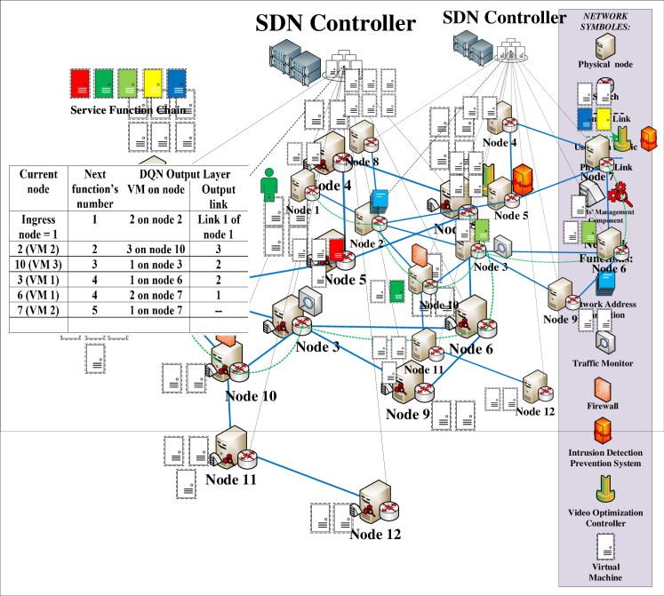
Figure 1: High level representation of the considered system model.

II-A Service Specification and Requirements

Based on the 3rd Generation Partnership Project (3GPP) standardization perspective [34], each communication service needs some NFs that run on the flow/packets of the services. European Telecommunications Standards Institute (ETSI) defines a set of NFs with specific chaining and descriptors as a Network Service (NS) [35] in the NFV environments. According to these, we consider a set of $K$ services which is denoted by $\mathcal{K}=\{1,\dots,K\}$ and a set of all NFs as $\mathcal{F}=\{1,\dots,F\}$. Each service $k$ has some NFs with specific ordering as an SFC that is shown in Fig. 2. We assume that $\mathcal{F}_{k}\subset\mathcal{F}$ is the set of specific functions of service $k$ like Firewall (FW), Network Address Translator (NAT), Intrusion Detection Prevention System (IDPS), and Video Optimization Controller (VOC). We assume that each service $k$ is specified by following:

$$R_{k}=\Big{(}n_{i,k},n_{e,k},B_{k},\tau_{k},\mathcal{D}_{k}\Big{)},\forall k\in\mathcal{K},$$ (1)

where $n_{i,k}$ and $n_{e,k}$ are the ingress and egress nodes of service $k$ [21, 36] and $\left\{n_{i,k},n_{e,k}\right\}\in\mathcal{N}$. It is worth mentioning that each of the services has a specific sequence of functions. For example, in the VoIP service, FW runs after NAT [37]. In addition, $B_{k}$ is the data rate in bits per second. Moreover, $\tau_{k}$ is the tolerable time which is dependent on the type of services of the top layer with respect to their latency requirements. Also, we define $d^{k}_{f}$ to determine the corresponding processing requirement for virtualized NF (VNF) $f$ in CPU cycle per bits of flow/packet in service $k$ [37]. Accordingly, for each service, we have a set of corresponding processing requirements as bellow:

$$\mathcal{D}_{k}=\{d_{{f}}^{k}\},\leavevmode\nobreak\ \leavevmode\nobreak\ \leavevmode\nobreak\ \leavevmode\nobreak\ \forall f\in\mathcal{F}_{k},\forall k\in\mathcal{K}.$$ (2)

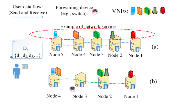
Figure 2: An example of SFC with different scenarios for function placement. We assume that the functions can placed on the successive nodes (a) or non successive nodes (b).

Table II: Main notations and parameters

Notation	Definition
$\mathcal{G(N,L)}$	Network graph
$\mathcal{N}/n$	Set/index of nodes
$\mathcal{L}$	Set of links
$\mathcal{U}/u$	Set/index of users
$\mathcal{F}/f$	Set/index of NFs
$\mathcal{F}_{k}$	Set NFs of service $k$
$\mathcal{V}/v$	Set/index of VMs
$\mathcal{P}/p$	Set/index of the physical paths
$\mathcal{E}/e$	Set/index of the virtual paths
$\boldmath{L}$	Connectivity matrix of graph
$x_{n,n^{\prime}}$	Capacity of the link between nodes $n$ and $n^{\prime}$ in bit per second
$w_{m,v}$	Weight/unit costs of VM $v$ on node $m$
$\hat{w}_{n,n^{\prime}}$	Weight/unit costs of the link between nodes $n$ and $n^{\prime}$
$n_{i,k},n_{e,k}$	The ingress and egress nodes of service $k$
$i^{p_{m,m^{\prime}}}_{n,n^{\prime}}$	Link indicator that shows that link between nodes
	$n$ and $n^{\prime}$ is placed on the physical path $p_{m,m^{\prime}}$
$B_{k}$	Data rate for service $k$ in bits per second
$\tilde{B}_{k}$	Packet size in bits
$\mathcal{D}_{k}$	Set of the corresponding processing
	requirement in CPU cycle per bit
	for the functions of service $k$
$d_{f}^{k}$	Corresponding processing requirement in CPU cycle per bit
	for function $f$ of service $k$
$\tau_{k}$	Tolerable latency of service $k$
$\xi_{v,m}^{f,u}\in\left\{0,1\right\}$	Selection indicator of VM $v$ for NF $f$ on node $m$ for user $u$
$\gamma$	Decay factor of reinforcement learning
$\alpha$	Learning rate for DQN
$\rho^{k,e^{v,v^{\prime}}_{m,m^{\prime}}}_{{p}_{m,m^{\prime}}}\in\left\{0,1\right\}$	Path selection variable that mapping the virtual
	path $e$ between virtual machine
	$v$ and $v^{\prime}$ for service $k$ to physical path $p_{n,n^{\prime}}$
	between nodes $n$ and $n^{\prime}$
$\Psi_{v,m}$	Processing resource at VM $v$
	on nodes $m$ in CPU cycle per second
$\delta_{u}^{k}$	Service request indicator where set to $1$
	for user $u$ that requests service $k$
${z}_{v,m}^{t}$	Available processing resource of VM $v$ that is
	raised on node $m$ at time slot $t$
${y}_{{n,n^{\prime}}}^{t}$	Available capacity resource of link between
	nodes $n$ and $n^{\prime}$ at time slot $t$

Also, to determine the order of the successive functions in a certain SFC, we define the order of functions by $f^{i}$ and $f^{i+1}$, where $f^{i}$ is $i$-th function of the SFC and $f^{i+1}$ is run after function $f^{i}$. To increase the readability of this paper, the main parameters and variables are summarized in Table II. Moreover, we consider a set $\mathcal{U}$ of users with different service requests. We assume that each user $u$ requests only one service. We define a binary indicator $\delta_{u}^{k}$, where if user $u$ requests service $k$, it is $1$ and otherwise $0$.

II-B Infrastructure Model

In order to model and formulate the NFV-enabled network, we consider graph $\mathcal{G}=(\mathcal{N},\mathcal{L})$, where $\mathcal{N}$ represents the set of nodes where $\left|\mathcal{N}\right|=N$ and $\mathcal{L}$ is the set of links between nodes. We further assume that each node $m$ hosts several VMs that is denoted by $\mathcal{V}_{m}=\{1_{m},\dots,V_{m}\}$ and created by a hypervisor, hence the set of total VMs in the network is denoted by $\mathcal{V_{\text{Total}}}=\cup_{m=1}^{N}\mathcal{V}_{m}$. In addition, we denote the maximum number of the VMs on each nodes by $V_{\text{max}}$.
Each VM $v$ on node $m$ has a specific processing resource that is denoted by $\Psi_{v,m}$ in CPU cycle per second. Hence, matrix $\bm{\Psi}=[\Psi_{v,m}]\in\mathbb{R}_{+}^{V\times N}$ indicates the amount of processing resources and also determine the VMs of each node. It is possible that each VM processes a set of NFs for different users based on the allowable capacity [9]. Moreover, we consider connectivity matrix as $\mathbb{L}=\left[l_{n,n^{\prime}}\right]$, that is defined as

$$\begin{split}&l_{n,n^{\prime}}=\begin{cases}1,&\text{a link between nodes $n$ and $n^{\prime}$ exists},\\ 0,&\text{otherwise}.\end{cases}\end{split}$$ (3)

Also, the link between nodes $n$ and $n^{\prime}$ has a limited bandwidth that is represented by matrix $\mathbb{X}=[x_{n,n^{\prime}}]\in{\mathbb{R}}_{+}^{N\times N}$, where $x_{n,n^{\prime}}$ is the capacity of link between nodes ${n}$ and ${n^{\prime}}$ in bits per second. Note that as the considered network is connected, there is at least one path between two nodes. Let $p_{m,m^{\prime}}$ denotes the $p$-th path between nodes $m$ and $m^{\prime}$. Therefore, we have a set $\mathcal{P}_{m,m^{\prime}}=\left\{1_{m,m^{\prime}},\dots,p_{m,m^{\prime}},\dots,P_{m,m^{\prime}}\right\}$ of all possible physical paths between nodes $m$ and $m^{\prime}$ such that each path contains a set of links. To determine which of the physical links are in a path, we define a link-to-path binary indicator as follows:

$$i^{p_{m,m^{\prime}}}_{n,n^{\prime}}=\begin{cases}1,&\text{the link between nodes $n$ and $n^{\prime}$}\\ &\text{ is in the path $p_{m,m^{\prime}},$}\\ 0,&\text{otherwise}.\end{cases}$$ (4)

Moreover, we consider the set of virtual paths between virtual machine $v$ and $v^{\prime}$ on nodes $m$ and $m^{\prime}$ as $\mathcal{E}^{v,v^{\prime}}_{m,m^{\prime}}=\left\{1^{v,v^{\prime}}_{m,m^{\prime}},\dots,e^{v,v^{\prime}}_{m,m^{\prime}},\dots,E^{v,v^{\prime}}_{m,m^{\prime}}\right\}$ where $e^{v,v^{\prime}}_{m,m^{\prime}}$ is the e-th path of this set [39], [40], and [41].

II-C Optimization Variables

We define a binary decision variable $\xi_{v,m}^{f^{i},k}$ to determine that $i$-th function of service $k$ is running on VM $v$ that is raised on node $m$ as follows:

$$\xi_{v,m}^{f^{i},k}=\begin{cases}1,&\text{ NF $f^{i}$ of service $k$ is running on VM $v$ in}\\ &\text{ node $m$,}\\ 0,&\text{otherwise}.\end{cases}$$ (5)

Moreover, to send data traffic of service $k$, we define a binary decision variable $\rho^{k,e^{v,v^{\prime}}_{m,m^{\prime}}}_{p_{m,m^{\prime}}}$ where it maps the virtual path $e^{v,v^{\prime}}_{m,m^{\prime}}$ to the physical path $p_{m,m^{\prime}}$ as follows:

$$\rho^{k,e^{v,v^{\prime}}_{m,m^{\prime}}}_{p_{m,m^{\prime}}}=\begin{cases}1,&\text{the physical path $p_{m,m^{\prime}}$ is selected to tarnsmit }\\ &\text{ of service the data traffic of service $k$ from}\\ &\text{ from virtual machine $v$ to $v^{\prime}$},\\ 0,&\text{otherwise},\end{cases}$$ (6)

where for each virtual path just one physical path is selected. Based on this, we define the following constraint:

$$\sum_{p_{m,m^{\prime}}\in\mathcal{P}_{m,m^{\prime}}}\rho^{k,e^{v,v^{\prime}}_{m,m^{\prime}}}_{p_{m,m^{\prime}}}=1,\forall k\in\mathcal{K}.$$ (7)

We note that the virtual path $e^{v,v^{\prime}}_{m,m^{\prime}}$ is between two successive functions of SFC of service $k$, $(f^{i},f^{i+1})$, with respect to the ordering of SFC. For example, in a certain service, the functions like web browsing, NAT function are always run before FW.
Moreover, the path between $n_{i,k}$ and the VM that the first function of SFC is placed is determined by $\hat{e}^{v}_{n_{i,k},n}$ and also for the path between the VM that the last function placed on it and $n_{e,k}$ is determined by $\hat{e}^{v}_{n,n_{e,k}}$.

II-D Delay Model

This work considers three types of delays as: 1) processing delay, 2) propagation delay and 3) transmission delay.

II-D1 Processing delay

The processing delay of NF $f$ on node $m$ for service $k$ in VM $v$ denoted by $\tau_{v,m}^{f,k}$ in seconds is given by

$$\tau_{v,m}^{f,k}=\frac{d_{{f}}^{k}\tilde{B}_{k}}{\Psi_{v,m}},\forall k\in\mathcal{K},v\in\mathcal{V}_{m},m\in\mathcal{N},$$ (8)

where $\tilde{B}_{k}$ is the packet size in bits. In this paper, we assume the packet size is equal to the number of bits transmitted in one second. For example, by considering a service with required $100$ Kbps data rate, the packet size is $100$ Kbits [9]. Also, the total of processing delay of service $k$ can be calculated by

$$D_{\text{Proc}}^{k}=\sum^{F_{k}}_{i=1}\sum_{m\in\mathcal{N}}\sum_{v\in\mathcal{V}_{m}}\xi_{v,m}^{f^{i},k}\tau_{v,m}^{f^{i},k},\forall k\in\mathcal{K},f^{i}\in\mathcal{F}_{k},\in\mathcal{K}.$$ (9)

II-D2 Propagation Delay

To formulate the propagation delay in the considered system, we define $\kappa_{n,n^{\prime}}$as the amount of propagation delay for the data traffic that traverses on link between nodes $n$ and $n^{\prime}$ depends on the length of this link and the speed of light. Therefore, the total propagation delay for service $k$ is obtained by:

$$D^{k}_{\text{Prop}}=\sum_{\begin{subarray}{c}{n,n^{\prime},m}\in\mathcal{N}\\ p_{n_{i,k},m^{\prime}}\in\mathcal{P}_{n_{i,k},m^{\prime}}\\ v\in\mathcal{V}_{m}\end{subarray}}\kappa_{n,n}i^{p_{n_{i,k},m}}_{n,n^{\prime}}\rho^{\hat{e}^{v}_{n_{i,k},m}}_{p_{n_{i,k},m}}\xi^{f^{1},k}_{v,m}+$$ (10)

$$\sum^{F_{k}-1}_{i=1}\sum_{\begin{subarray}{c}{n,n^{\prime},m^{\prime},m^{\prime\prime}}\in\mathcal{N}\\ p_{m^{\prime},m^{\prime\prime}}\in\mathcal{P}_{m^{\prime},m^{\prime\prime}}\\ v^{\prime},v^{\prime\prime}\in\mathcal{V}_{m}\end{subarray}}\kappa_{n,n^{\prime}}i^{p_{m^{\prime},m^{\prime\prime}}}_{n,n^{\prime}}\rho^{e^{v^{\prime},v^{\prime\prime}}_{m^{\prime},m^{\prime\prime}}}_{p_{m^{\prime},m^{\prime\prime}}}\xi^{f^{i},k}_{v^{\prime},m^{\prime}}\xi^{f^{i+1},k}_{v^{\prime\prime},m^{\prime\prime}}+$$

$$\sum_{\begin{subarray}{c}n,n^{\prime},m^{\prime\prime\prime}\in\mathcal{N}\\ p_{m^{\prime\prime\prime},n_{e,k}}\in\mathcal{P}_{m^{\prime\prime\prime},n_{e,k}}\\ {v^{\prime\prime\prime}\in\mathcal{V}_{m}}\end{subarray}}\kappa_{{n,n^{\prime}}}i^{p_{m^{\prime\prime\prime},n_{e,k}}}_{{n,n^{\prime}}}\rho^{\hat{e}^{v^{\prime\prime\prime}}_{m^{\prime\prime\prime},n_{e,k}}}_{p_{m^{\prime\prime\prime},n_{e,k}}}\xi^{f^{F_{k}},k}_{v^{\prime\prime\prime},m^{\prime\prime\prime}},$$

$$\forall k\in\mathcal{K}.$$

In the first term of (10), we calculate the propagation delay between $n_{i,k}$ and the first VM that the first function is placed. In addition, the second term calculate the propagation delay of the link between the next functions. Finally the last term calculates the propagation delay on the link between the last VM that and $n_{e,k}$.

II-D3 Transmission Delay

The total transmission delay of service $k$ is calculated by:

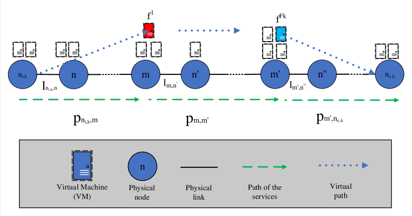
Figure 3: The illustration of equations (10) and (II-D3) for calculation of propagation and transmission delay. These equations are included three terms that calculate the propagation and transmission delay between the ingress nodes and the first VM’ node and the last VM’s node and egress node of services.

$$D_{\text{Tran}}^{k}=\sum_{\begin{subarray}{c}{n,n^{\prime},m}\in\mathcal{N}\\ p_{n_{i,k},m}\in\mathcal{P}_{n_{i,k},m}\\ {v\in\mathcal{V}_{m}}\end{subarray}}i^{p_{n_{i,k},m}}_{n,n^{\prime}}\rho^{k,\hat{e}^{v}_{n_{i,k},m}}_{p_{n_{i,k},m}}\xi^{f^{1},k}_{v,m}\frac{\tilde{B}_{k}}{x_{n,n^{\prime}}}+$$

$$\sum^{F_{k}-1}_{i=1}\sum_{\begin{subarray}{c}{n,n^{\prime},m^{\prime},m^{\prime\prime}}\in\mathcal{N}\\ p_{m^{\prime},m^{\prime\prime}}\in\mathcal{P}_{m^{\prime},m^{\prime\prime}}\\ {v^{\prime},v^{\prime\prime}\in\mathcal{V}_{m}}\end{subarray}}i^{p_{m^{\prime},m^{\prime\prime}}}_{{n,n^{\prime}}}\rho^{k,e^{v^{\prime},v^{\prime\prime}}_{m^{\prime},m^{\prime\prime}}}_{p_{m^{\prime},m^{\prime\prime}}}\xi^{f^{i},k}_{v^{\prime},m^{\prime}}\xi^{f^{i+1},k}_{v^{\prime\prime},m^{\prime\prime}}\frac{\tilde{B}_{k}}{x_{n,n^{\prime}}}+$$

$$\sum_{\begin{subarray}{c}n,n^{\prime},m^{\prime\prime\prime}\in\mathcal{N}\\ p_{m^{\prime\prime\prime},n_{e,k}}\in\mathcal{P}_{m^{\prime\prime\prime},n_{e,k}}\\ v^{\prime\prime\prime}\in\mathcal{V}_{m}\end{subarray}}i^{p_{m^{\prime\prime\prime},n_{e,k}}}_{{n,n^{\prime}}}\rho^{k,\hat{e}^{v^{\prime\prime\prime}}_{m^{\prime\prime\prime},n_{e,k}}}_{p_{m^{\prime\prime\prime},n_{e,k}}}\xi^{f^{F_{k}},k}_{v^{\prime\prime\prime},m^{\prime\prime\prime}}\frac{\tilde{B}_{k}}{x_{n,n^{\prime}}},$$ (11)

$$\forall k\in\mathcal{K},\forall f^{i}\in\mathcal{F}_{k}.$$

To have better understanding and realization of (II-D3) and (10), the details of these equations are depicted in Fig. 3. Based on the formulated latency, the total delay for each packet of service $k$ is obtained as:

$$D_{\text{Total}}^{k}=D_{\text{Proc}}^{k}+D_{\text{Prop}}^{k}+D^{k}_{\text{Tran}},\forall k\in\mathcal{K}.$$ (12)

II-E Objective Function

We define a weighted cost function that includes the cost of processing and bandwidth resources at the level of VMs and links that is given by:

$$\phi(\bm{\rho},\bm{\xi})=\sum_{k\in\mathcal{K}}\sum_{\begin{subarray}{c}{u\in\mathcal{U}}\\ {m\in\mathcal{N}}\\ {v\in\mathcal{V}_{m}}\\ {f\in\mathcal{F}_{k}}\end{subarray}}w_{m,v}d_{{f}}^{k}{B}_{k}\delta_{u}^{k}\xi_{v,m}^{f,k}+$$ (13)

$$\sum_{k\in\mathcal{K}}\sum_{\begin{subarray}{c}{u\in\mathcal{U}}\\ {n,n^{\prime},m,m^{\prime}\in\mathcal{N}}\\ p_{m,m^{\prime}}\in\mathcal{P}_{m,m^{\prime}}\\ v,v^{\prime}\in\mathcal{V}_{m}\end{subarray}}\hat{w}_{{n,n^{\prime}}}\delta^{k}_{u}i^{p_{m,m^{\prime}}}_{n,n^{\prime}}\rho^{k,e^{v,v^{\prime}}_{m,m^{\prime}}}_{p_{m,m^{\prime}}}\xi^{f,k}_{v,m}\xi^{f^{\prime},k}_{v^{\prime},m^{\prime}}B_{k},$$

where $w_{m,v}>0$ denotes the unit cost of VM $v$ on node $m$ that converts the utilized resources to the cost. By considering the service bandwidth and the processing requirement for each of the functions that are placed in the VMs, the total processing cost is calculated by the first term. Subsequently, $\hat{w}_{n,n^{\prime}}>0$ denotes the unit cost of the link between nodes $n$ and $n^{\prime}$. By considering the links that are included in the selected paths and the bandwidth of the requested services, the total bandwidth utilization cost is calculated by the second term.
The values of parameters $w_{m,n}$ and $\hat{w}_{n,n^{\prime}}$ depend on the type of nodes, and links, for example, the edge or core nodes has different (cost) weights. Based on the definitions, our main aim is to solve the following optimization problem:

$$\min_{\bm{\rho},\bm{\xi}}\;\phi$$ (14a)

s.t. $$\sum_{m,m^{\prime}\in\mathcal{N}}i^{p_{m,m^{\prime}}}_{{n,n^{\prime}}}\rho^{k,e^{v,v^{\prime}}_{m,m^{\prime}}}_{p_{m,m^{\prime}}}B_{k}\leq x_{n,n^{\prime}},\forall k\in\mathcal{K},$$ (14b)

$$\forall v,v^{\prime}\in\mathcal{V}_{m},\forall n,n^{\prime}\in\mathcal{N},$$

$$\sum_{m\in\mathcal{N}}\xi^{f^{i},k}_{v,m}d^{f}_{k}B_{k}\leq\Psi_{v,m},f^{i}\in\mathcal{F}_{k},\forall k\in\mathcal{K},\forall v\in\mathcal{V}_{m},$$ (14c)

$$\sum_{m\in\mathcal{N}}\sum_{v\in\mathcal{V}_{m}}\xi_{v,m}^{f^{i},k}=1,\leavevmode\nobreak\ \forall k\in\mathcal{K},f\in\mathcal{F}_{k},$$ (14d)

$$D_{\text{Total}}^{k}\leq\tau_{k},\leavevmode\nobreak\ \leavevmode\nobreak\ \leavevmode\nobreak\ \leavevmode\nobreak\ \leavevmode\nobreak\ \leavevmode\nobreak\ \leavevmode\nobreak\ \forall k\in\mathcal{K},$$ (14e)

$$\xi_{v,m}^{f^{i},k}\in\{0,1\},\leavevmode\nobreak\ \leavevmode\nobreak\ \leavevmode\nobreak\ \leavevmode\nobreak\ \leavevmode\nobreak\ v\in\mathcal{V}_{m},f\in\mathcal{F}_{k},m\in\mathcal{N},\forall k\in\mathcal{K},$$ (14f)

$$\rho^{k,e^{v,v^{\prime}}_{m,m^{\prime}}}_{{p}_{m,m^{\prime}}}\in\left\{0,1\right\},\leavevmode\nobreak\ \leavevmode\nobreak\ \leavevmode\nobreak\ \forall k\in\mathcal{K},p_{m,m^{\prime}}\in\mathcal{P}_{m,m^{\prime}},$$ (14g)

where $\bm{\rho}=[\rho^{k,e^{v,v^{\prime}}_{m,m^{\prime}}}_{{p}_{m,m^{\prime}}}]$ and $\bm{\xi}=[\xi_{v,m}^{f,k}]$. Constraint (14b) ensures that the total resources allocated to service $k$ in all links in path $p_{m,m^{\prime}}$ are less that the link capacity. Constraint (14c) ensures that the total resources allocated to all users are less than the processing capacity of VM $v$ on node $m$. Constrain (14d) indicates that each NF is assigned to one VM. By (14e), we consider that the total delay is less than the predefined tolerable latency of the services.

III PROPOSED SOLUTION

Problem (14) is a integer linear problem witch is complicated to solve efficiently. Therefore, we adopt an RL-based algorithm to solve it. Adopting a RL-based solution for solving problem (14) is a challenge that has significant effect on the obtained results. In this section, first, we evaluate the basic principles of RL algorithms, and second, we describe how to adopt these principles to solve the proposed problem.

III-A Proposed DQN Adaptive Resource (DQN-AR) Allocation Algorithm

We propose a RL-based RA algorithm with considering the basic concepts of RL. The basics of RL are agent, state, action, reward, and an environment. The agent in each iteration, with considering the state of the environment, selects an action that causes that the state changes into the next state. Subsequently, to evaluate the performance of each action, the agent gets a reward from the environment. The set of states, actions, rewards and next state is collocated in each step of RL based algorithm to the agent, so that based on these experiments, the agent can select better actions in the same states. Based on the mentioned assumptions, the main equation for the $Q$-learning algorithm is defined as follows [42]:

$$Q(s^{t},a^{t})\leftarrow Q(s^{t},a^{t})+$$ (15)

$$\alpha\left[r^{t}+\gamma\operatorname*{arg\,max}_{a^{\prime}}\left(Q(s^{t+1},a^{\prime})-Q(s^{t},a^{t})\right)\right],$$

where $s^{t}$, $a^{t}$, and $r^{t}$ denote the state, action, and the obtained reward in the $t$-th step, respectively. In addition, the learning rate and discount factor are denoted by $\alpha$ and $\gamma$, respectively. Because deploying $Q$-learning for the huge state-action space is not possible [17], [30], a DNN is deployed for estimating the $Q$-function values.
Based on the mentioned above, we consider the network components as the basics of components RL.
Descriptions of DQN: We adopt Algorithm 2 where the DQN algorithm chooses a random action with probability $\epsilon$. The parameter $\epsilon$ is set to $1$ in the first iteration and has a final value, $\epsilon=0.1$ whereas the decay coefficient of epsilon is set to $0.9$. To make sure that the algorithm does not get the local optimum, in each time slot with probability $0\leq\epsilon<1$, we choose a random action [43]. In fact, $\epsilon$ parameters determine the ratio between exploration and exploitation in the search algorithm [42]. In addition, we store the current sate, action, new state, and reward in $\mathcal{\hat{D}}$ memory with a certain size. To update the parameters of DQN, we sample the set $\hat{\mathcal{B}}$ of the transactions with the number $|\hat{\mathcal{B}}|$. We set the memory size $|\hat{\mathcal{D}}|=2000$ for storing transactions and the size of mini-batch $\hat{\mathcal{B}}$ is set to $8$ transactions [25]. The learning rate $\alpha$ and the discount factor $\gamma$ is set to $0.001$ and $0.95$, receptively [7, 43]. The reason for using a discount factor $\gamma$ is that it prevents the total reward from going to infinity [44].
$\bullet$ Agent: We consider the SDN controller as the agent that by considering the network’s states, chooses the actions form action spaces. For each selected action, the agent gets a reward and the network’ state changes to the next state over the time. To have a smart and adaptive algorithm, the agent needs to have knowledge about the network state and condition in each time slot $t$. For this reason, available resources or capacity of nodes and links at each time slot $t$ is necessary [29]. To this end, we propose a available calculation algorithm that more details follow in Algorithm 1.
$\bullet$ Network States: We denote the state space at each time slot $t$ by $\bm{S}^{t}$ as network resources that includes the available resources in terms of processing resources of VMs and links’ bandwidth as follows:

$$\bm{S}^{t}=(\mathbb{Z}^{t},\mathbb{Y}^{t}),$$ (16)

$$\mathbb{Z}^{t}=[z_{v,m}^{t}]\in\mathbb{R}_{+}^{V\times N}, \mathbb{Y}^{t}=[y_{{n,n^{\prime}}}^{t}]\in\mathbb{R}_{+}^{N\times N},$$

where $z_{v,m}^{t}$ and $y_{n,n^{\prime}}^{t}$ are the available processing resource of VM $v$ on physical node $m$ and bandwidth of link between nodes ${n}$ and ${n^{\prime}}$ in time slot $t$, respectively, and obtained by Algorithm 1. First, we divide the amount of each resource to $I$ levels. To represent the resources state, we normalized the gap between beginning time and time slot $t$ as bellow [29]:

$${s}^{t}_{{n,n^{\prime}}}=\lfloor I\frac{y_{{n,n^{\prime}}}^{0}-y_{{n,n^{\prime}}}^{t}}{y_{{n,n^{\prime}}}^{0}}\rfloor,\leavevmode\nobreak\ \leavevmode\nobreak\ \leavevmode\nobreak\ \leavevmode\nobreak\ \leavevmode\nobreak\ s_{v,n}^{t}=\lfloor I\frac{z_{v,n}^{0}-z_{v,n}^{t}}{z_{v,n}^{0}}\rfloor.$$ (17)

In order to apply resources’ state to input of the DQN, the values of each network component (links and VMs) are normalized. In addition, we set $I$ to 1000 [7]. In addition, in RA algorithm, the agent considers the service specification, the previous selected node and VM in the path from ingress to egress nodes, and order of the function in SFC as state. Moreover, we assume that in each time slot $t$, the agent has some steps to choose action and perform the RA algorithm. We denote the state and action at time slot $t$ and step $j$, for service $k$, by $s^{t,j}$ and $a^{t,j}_{k}$, respectively. To ensure a limited solving time in each time slot, we assume a upper bound for the steps that is denoted by $J$ and it is set to $100$ in each time slot.
$\bullet\leavevmode\nobreak\$Calculating Available Resources: As mentioned before, we need to have an algorithm that returns the available resources at each time slot. Based on service duration time, the service of users is terminated and their resources are released. Also, to calculate the available resources, it is outlined in Algorithm 1.

Input: The network graph and capacity of the links and VMs; $\mathcal{G}$, $\bm{\Psi}$, and $\mathbb{X}$

1 for  each time slot $t$ do

2       for  each services $k$ do

3             for  each users $u$ do

4                  Save the arrival time ${t}_{u}$ for user $u$

5                   if the request accepted (By the Actions) then

6                         if at the begining time then

7                              $z_{v,m}^{t_{u}}=\Psi_{v,m}-d_{f}^{k}B_{k}\xi_{v,m}^{f,k}$

8                               $y^{t_{u}}_{{n,n^{\prime}}}=x_{n,n^{\prime}}-B_{k}i^{p_{m,m^{\prime}}}_{n,n^{\prime}}\rho^{k,e^{v,v^{\prime}}_{m,m^{\prime}}}_{p_{m,m^{\prime}}}$

9                               else

10                                    $z_{v,m}^{t_{u}}=z_{v,m}^{t_{u}-\hat{t}}-d_{f}^{k}B_{k}\xi_{v,m}^{f,k}$

11                                     $y^{t_{u}}_{{n,n^{\prime}}}=y^{t_{u}-\hat{t}}_{{n,n^{\prime}}}+B_{k}i^{p_{m,m^{\prime}}}_{n,n^{\prime}}\rho^{k,e^{v,v^{\prime}}_{m,m^{\prime}}}_{p_{m,m^{\prime}}}$

12                              if  the user departure then

13                                    Release the user $u$ resource’s

14                                     $z_{v,m}^{t}=z_{v,m}^{t_{u}}+d_{f}^{k}B_{k}\xi_{v,m}^{f,k}$

15                                     $y^{t}_{n,n^{\prime}}=y^{t_{u}}_{{n,n^{\prime}}}+B_{k}i^{p_{m,m^{\prime}}}_{n,n^{\prime}}\rho^{k,e^{v,v^{\prime}}_{m,m^{\prime}}}_{p_{m,m^{\prime}}}$

16                                     ${t}_{u}\leftarrow 0$

17                              Update State :$\mathbb{Z}^{t}$, $\mathbb{Y}^{t}$ according to the utilization of links and nodes based on the bandwidth and processing resources

18                        

19                  

20            

      Output: $\mathbb{Z}^{t},\,\mathbb{Y}^{t}$

21      

Algorithm 1 Resource Allocation and Calculating of Available Resources

1 Initialize the DNN with random weights and consider the network graph and capacity of the links and VMs; $\mathcal{G},\bm{\Psi},\mathbb{X},\text{and set the initial weighth for DNN}:\leavevmode\nobreak\ \theta_{0}$

2 if the central controller want taking an action then

3      Action $a^{t,j}_{k}$ is selected;

4       $a^{t,j}_{k}=\begin{cases}\text{ select a random action}&\text{with probability}\leavevmode\nobreak\ \epsilon,\\ \operatorname*{arg\,max}_{a}(Q(s^{t,j},a))&\text{with probability}\leavevmode\nobreak\ 1-\epsilon\end{cases}$

5       Store transaction ($s^{t,j},a^{t,j}_{k},r^{t,j}_{k},s^{t+1,j}$) in memory $\mathcal{\hat{D}}$

6       Sample random minibatch with batch size $\hat{\mathcal{B}}$ of transitions $(s^{t,j},a^{t,j}_{k},r^{t,j}_{k},s^{t+1,j})$ from $\mathcal{\hat{D}}$

7if a request accepted then

8      Perform Algorithm 1

9else

10      Perform gradient descent step on Mean Square Erorr (MSE) of $(r^{t,j}_{k}-Q(s^{t,j},a^{t,j}_{k};\theta))^{2}$ and update parameter $\theta^{t}$ of network

Algorithm 2 DQN Algorithm

Action Space: The action space is denoted by $\mathcal{A}$ which includes all the network VMs on the nodes that can be considered for function placement or as a switch. Based on the network state and SFC requirements, a subset of actions is possible that is denoted by $\mathcal{A}_{p}\subset\mathcal{A}$. For example, if user $u$ requests service chain $\left\{f^{1}\rightarrow f^{2}\rightarrow f^{3}\right\}$, the corresponding action determines that the next node and VM is selected for function placement or just it is a switch. In fact, we propose a smart and adaptive NFV-RA algorithm that perform joint function placement and node by node dynamic routing. More details are given in Algorithm 3. Thus, the size of all action space for each of service request is calculated by

$$|\mathcal{A}|=|\mathcal{N}|\times|\mathcal{V}_{\text{Total}}|\times 2.$$ (18)

Consequently, the agent for user $u$ in the service $k$ selects action $a^{t,j}_{k}\in\mathbb{N}$ at time slot $t$ in $j$th step of Algorithm 3.
$\bullet$ DQN-AR for RA, Dynamic Routing, and Function Placement: To adopt Algorithm 2 for dynamic routing and function placement, we propose an algorithm that by an interactive approach with Algorithm 2, performs a node by node routing and function placement beginning from $n_{i,k}$ and in each step of routing algorithm, considers the current node as $n_{c,k}$ and continues to reach $n_{e,k}$. On the other hand, for each of service requests, with considering the network state and service specification as inputs of DQN, the output of the DQN determines the corresponding action as the next node and VM in SFC path. It is worth mention that in each step, only a set of the actions is possible. We consider the set of nodes that are directly connected to current node $n_{c,k}$ and it is denoted by $\mathcal{N}_{c,k}$. Subsequently, we consider the set of VMs in which they are on the set $\mathcal{N}_{n,c}$ as set of the possible actions and it is denoted by $\hat{\mathcal{N}}_{c,k}$. In addition, we assume that the agent can choose a VM form $\hat{\mathcal{N}}_{c,k}$. The agent can placed a function on the selected VM or consider the selected VM as a forwarding device. Furthermore, we assume $\mathcal{A}_{p,p}=\mathcal{A}_{p,s}=\left\{\hat{\mathcal{N}}_{n_{c,k}}\right\}$ where $\mathcal{A}_{p,p}$ and $\mathcal{A}_{p,s}$ are the sets of possible actions for function placement and router selection, respectively. Thus, the set of possible action is defined by $\mathcal{A}_{p}=\mathcal{A}_{p,p}\cup\mathcal{A}_{p,s}$. To determine the type of each action, we define an auxiliary binary variable as $a^{t,k}_{s,k}$ as follows:

$$a^{t,k}_{s,k}=\begin{cases}0,\leavevmode\nobreak\ \leavevmode\nobreak\ \text{If}\leavevmode\nobreak\ \leavevmode\nobreak\ a^{t,k}_{k}\equiv_{2}0,\\ 1,\leavevmode\nobreak\ \leavevmode\nobreak\ \text{otherwise}.\end{cases}$$ (19)

It is worth to mention that, if the agent chooses a possible action, $(a^{t,j}_{k}\in{\mathcal{A}}_{p})$, the sub action $a^{t,j}_{s,k}$ determines the type of each action. Based on this, type of each action is defined by

$$a^{t,j}_{k}\in\begin{cases}\mathcal{A}_{p,p},&a^{t,j}_{s,k}=1,\\ \mathcal{A}_{p,s},&\text{otherwise}.\end{cases}$$ (20)

In each step, if the selected action is possible, then we check that this action belongs to which set. If constraints (14c) and (14b) are satisfied, the function is placed on selected VM on corresponding node otherwise the request is rejected. Similarly, for the links, we check the constraint (14b) sanctification. Nevertheless, the processing and propagation delay that incur the action $a^{t,j}_{k,u}$ is denoted by $\hat{\tau}$ and calculated by

$$\hat{\tau}=\begin{cases}\tau^{f,k}_{v,m}+i^{p_{m,m^{\prime}}}_{n,n^{\prime}}\rho^{k,e^{v,v^{\prime}}_{m,m^{\prime}}}_{p_{m,m^{\prime}}}\kappa_{{n,n^{\prime}}},\leavevmode\nobreak\ \leavevmode\nobreak\ \leavevmode\nobreak\ &a^{t,k}_{s,j}=1,\\ i^{p_{m,m^{\prime}}}_{n,n^{\prime}}\rho^{k,e^{v,v^{\prime}}_{m,m^{\prime}}}_{p_{m,m^{\prime}}}\kappa_{{n,n^{\prime}}},\leavevmode\nobreak\ \leavevmode\nobreak\ \leavevmode\nobreak\ &\text{otherwise}.\end{cases}$$ (21)

In each step, by checking constraints (14e), we ensure the tolerable time of service request.
$\bullet$ Reward Function: The agent after doing action $a^{t,j}_{k}$ obtains a reward that is denoted by $r^{t,j}_{k}$ in $j$th step of the RA algorithm to service $k$ in time slot $t$. Nevertheless, the agent selects a VM on a node for function placement or as forwarding device in $j$th step of Algorithm 3. Subsequently, if the link between the current node, and the next node and processing capacity of the next node’s VM satisfy constraints (14b), (14c) and (14e), the agent obtains reward that is calculate by the following:

$$r^{t,j}_{k}=w_{acc}-w_{cost}\tilde{\phi}^{j}_{k}\leavevmode\nobreak\ \leavevmode\nobreak\ \leavevmode\nobreak\ ,\forall k\in\mathcal{K},\forall t,$$ (22)

where $w_{acc}$ and $w_{cost}$ are coefficient factors of constraint satisfaction and cost and $\tilde{\phi}^{j}_{k}$ is the cost of the action, given below:

$$\tilde{\phi}^{j}_{k}=a^{t,k}_{s,k}w_{m,v}d^{k}_{f}B_{k}\delta^{k}_{u}\xi^{f,k}_{v,m}+$$ (23)

$$\hat{w}_{{n,n^{\prime}}}B_{k}i^{p_{m,m^{\prime}}}_{n,n^{\prime}}\rho^{k,e^{v,v^{\prime}}_{m,m^{\prime}}}_{p_{m,m^{\prime}}},\forall u\in\mathcal{U},\forall f\in\mathcal{F}_{k},\forall k\in\mathcal{K}.$$

Otherwise, if the constraints are not satisfied, the request is rejected and the agent reward is set to $0$. Based on this the reward of each step $j$ is calculated by following:

$$r^{t,j}_{k}=\begin{cases}w_{acc}-w_{cost}\tilde{\phi}^{j}_{k},\leavevmode\nobreak\ \leavevmode\nobreak\ \leavevmode\nobreak\ &\text{if the constraints satisfied},\\ 0,\leavevmode\nobreak\ \leavevmode\nobreak\ \leavevmode\nobreak\ \leavevmode\nobreak\ \leavevmode\nobreak\ \leavevmode\nobreak\ \leavevmode\nobreak\ \leavevmode\nobreak\ \leavevmode\nobreak\ \leavevmode\nobreak\ &\text{otherwise}.\end{cases}$$ (24)

In fact, for each step $j$ of the Algorithm 3, we define a reward that depends on constraints sanctification and cost of each action. Finally, the total reward that the agent obtained is defined by

$$r^{t}_{k}=\sum_{j}r^{t,j}_{k}.$$ (25)

1 for each time slot $t$ do

2       for each service $k$ do

3             $t_{u}\leftarrow$Arivial time, $t_{o}\leftarrow 0,\ i_{f}\leftarrow 0$, $j\leftarrow 0$, $\hat{p}=\left\{\right\}$, $n_{c,k}\leftarrow n_{i,k}$

4             while Constraint (14e) is satisfied, $t_{o}<\tau_{k}$ do

5                  while $n_{c,k}\neq n_{e,k}$ do

6                        while $j<J$ do

7                               if $a^{t,j}_{k,u}\in\mathcal{A}_{p}$ then

8                                     $\hat{p}\leftarrow\hat{p}\bigcup\left\{a^{t,j}_{k}\right\}$

9                                     if $a^{t,j}_{k}\in\mathcal{A}_{p,p}$ then

10                                          if $i_{f}<F_{k}$ then

11                                                if Constraints (14c) and (14b) are satisfied then

12                                                      Calculate $r^{t,j}_{k}$

13                                                      $i_{f}\leftarrow i_{f}+1$, $f\leftarrow f^{\prime},j\leftarrow j+1,t_{o}\leftarrow t_{o}+\hat{\tau}$

14                                                else

15                                                      request is rejected

16                                                      $r^{t}_{k}\leftarrow 0$

17                                                

18                                          else

19                                                consider $a^{t,j}_{k}$ as switch

20                                                 $j\leftarrow j+1,t_{o}\leftarrow t_{o}+\hat{\tau}$

21                                          

22                                    else

23                                          if Constraint (14b) is satisfied then

24                                                Calculate $r^{t,j}_{k}$

25                                                $j\leftarrow j+1,t_{o}\leftarrow t_{o}+\hat{\tau}$

26                                          

27                                    

28                              

29                        else

30                              request is rejected

31                              $r^{t}_{k}\leftarrow 0$

32                        

33                  if $i_{f}<F_{k}$ then

34                        if Constraint (14c) and $i_{f}<F_{k}$ then

35                              Function $f$ is placed on engress node;

36                              Calculate $r^{t,j}_{k}$

37                              $i_{f}\leftarrow i_{f}+1$, $f\leftarrow f^{\prime}$, $j\leftarrow j+1,t_{o}\leftarrow t_{o}+\hat{\tau}$

38                        

39                  

40            if $t_{o}>\tau_{k}$ then

41                  request is rejected

42                  $r^{t}_{k}\leftarrow 0$

43            

44      

Algorithm 3 DQN-based NFV-RA algorithm for dynamic routing and function placement

The designed DQN is depicted in Fig. 5. According to the figure, by considering the network state as DQN input, the DNN output layer determines the actions. Note that some of the nodes in the path are only forwarding devices (e.g., switch) (see Fig. 2 and 4).

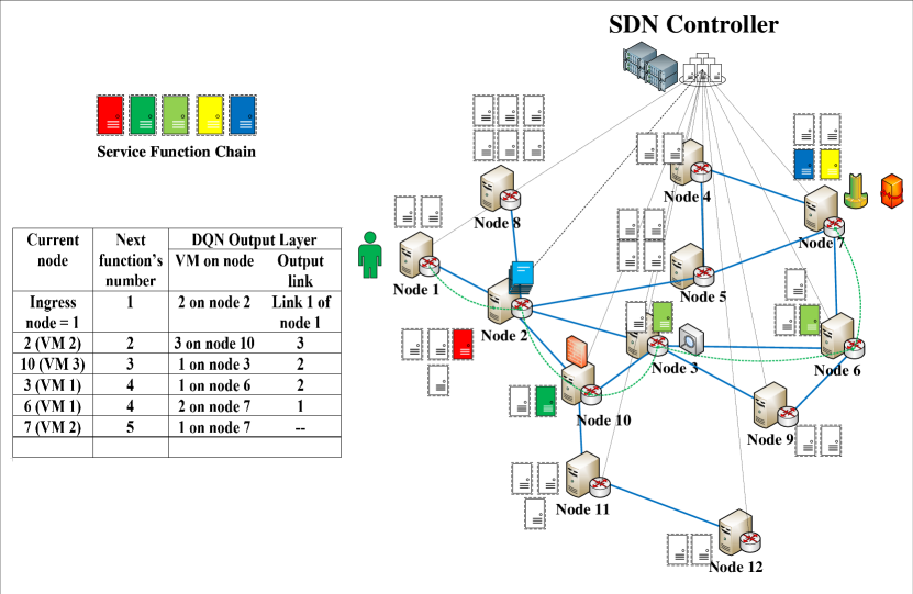
Figure 4: An example of function placement and node by node routing algorithm for a specific service

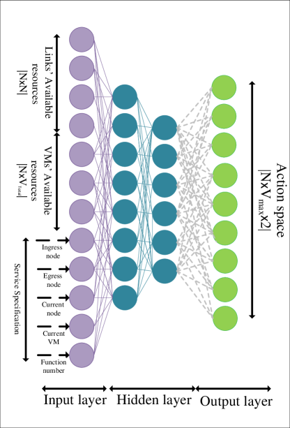
Figure 5: The DQN based on the network state and service specification determines the action.

IV COMPUTATIONAL COMPLEXITY

We analyze the computational complexity of the proposed DQN-AR algorithm and then we compare it with the NFV deep algorithm [7], Tabu search algorithm [45], and greedy search algorithm which is the well know algorithm that is deployed in [46, 47, 48]. The complexity of DNN based algorithms is depended on the architecture, configuration, number of input and output, and hidden layers. Moreover, for deploying DNN in the DQN-AR algorithm, considering the action space size and state space size is required [7]. Also, by considering the number of output layer neurons as $P_{o}$, number of the input layer neurons as $P_{i}$, and number of the hidden layers as $P_{h}$, the time complexity of the proposed DQN-AR for each action is obtained by following:

$$\mathcal{O}(P_{n}\times(P_{i}+P_{h}\times P_{n}+P_{o})),$$ (26)

where $P_{n}$ is the hidden layer’s neuron number [29]. Also, as can be seen from Fig. 5, $P_{i}=|\mathcal{L}|+|\mathcal{N}|\times|\mathcal{V}_{\text{Total}}|+5$ and $P_{o}=|\mathcal{N}|\times|\mathcal{V}_{\text{Total}}|\times 2$. Moreover, by considering $E$ iterations in the case of Tabu search, for $|\mathcal{K}|$ number of service requests, the time complexity is obtained by $\mathcal{O}(E\times|\mathcal{K}|\times F)$ for $F$ number of functions in a certain SCF. Accordingly, by increasing the number of iterations, the complexity of the Tabu search is increasing that can cause more complexity in the case of problems with a larger space of feasible solutions. Finally, to find the shortest path from ingress node to egress nodes for each of services with $F$ functions, in a network with $|\mathcal{N}|$ nodes and $|\mathcal{L}|$ links, the total time complexity is obtained by $\mathcal{O}(|\mathcal{K}|\times(|\mathcal{L}|+|\mathcal{N}|\log(|\mathcal{N}|)+F\times K)$.

V SIMULATION RESULTS

We analyze the performance of the proposed method using simulations. Accordingly, first we investigate the convergence of the proposed method. Next, we evaluate the effect of the coefficient factors in the the objective function. Afterwards, we compare the results of the proposed method with the baselines.

V-A Simulation Setup

Table III: Simulation Setting

Parameters	Value
	Average Duration Time:
	240, 600, 900, 1200 seconds [29]
	Data Rate:
	Max = 4 Mbps Min = 64Kbps [37]
	Average Tolerable Time
	Max = 500ms Min = 100ms
	VNF and Services:
Service Specification	FW, NAT, IDNS, TM, VOC [37]
	Web Browsing, Voice over IP, Video Streaming
	VM’s Capacity:
	Max = 1200 CPU Cycle per second Min = 200 CPU Cycle per second [40]
	Link’s Capacity:
Network Resources	Max = 6400 Mbps Min = 1600 Mbps [40]
	Number of the Server Node:
	10, 20, 30, 50, 100 [7]
	Propagation delay on the links
	Max = 15ms Min = 5ms
	Number VMs of each nodes
Network Configuration	$V_{\text{max}}$=6

As listed in Table. III, we consider some of the service specifications based on their QoSs [37] and service lifetime. We assume that each time slot is equal to one second. We consider $1000$ to $6000$ time slots for the simulation time, and $2000$ iterations [7] with $10$ Monte Carlo repetitions. Moreover, we generate the number of service requests by the Uniform random process [20] and the service life time by the exponential random process. Also, to set the ingress and egress nodes for set $\mathcal{K}$, at the beginning of the simulation, we select some random nodes among the network nodes.
Subsequently, to have a network with certain number of edges and nodes, we generate a random connected graph through NetworkX libraries in Python [25], [40]. Also, to deploy DNN, we use Tensorflow and Keras libraries in Python. Moreover, for the cost weight, we consider $w_{n,v}$ and $\hat{w}_{n,n^{\prime}}$ in range of $25$ to $75$ $/Mbps [9]. In addition, the source code of the proposed DQN-AR is available in [49].

V-B Simulation Results Discussions

We evaluate the effect of the main parameters, such as, services’ life time, number of the server nodes of the network (network topology), and the number of the arrival service requests on different baseline algorithms.

V-B1 Average Acceptance Ratio (AAR)

As the network topology, such as the number of the nodes and links and their configurations, has a significant effect on the routing algorithm and protocols, we evaluate the AAR on different network typologies. To have a comparison of the effect of the network topology on the performance of the agent, we consider the networks with size 10 to 100 nodes to evaluate the AAR over the iteration number. As can be seen in Fig. 6, in the first iteration, the AAR for the different network typologies have significant differences, specially, in the networks with large number of the server nodes. It is because that in a large network, the agent needs to select more actions to find appropriate path from ingress node to egress node and also the SFC placement on the VMs for each service request. Gradually, the AAR increases over the iterations. That is because the agent learns how to handle the requests and find the appropriate path from ingress nodes into egress nodes in different states.

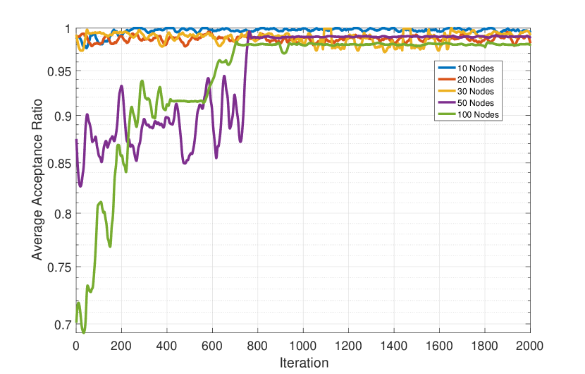
Figure 6: AAR over the iterations for different network topology

V-B2 Average Network Utilization Cost (ANUC)

Network topology and configuration have a significant effect on the length of the paths. To evaluate the effect of the network topology on the ANUC, we consider the network with 10 to 100 nodes. Because of the significant differences in the length of the paths from ingress to egress nodes in small and big networks, ANUC depends on the network size as shown in Fig. 7. Since the initial actions are selected by the agent randomly, we see that the obtained utilization cost is very high. After that, the agent gets more experience and take the actions based on the obtained experience and the ANUC gradually decreases over the iterations.

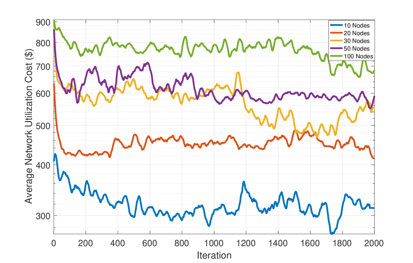
Figure 7: ANUC over the iterations for different network topologies

V-C Baselines Algorithms

In order to evaluate the performance of the proposed DQN-AR, we consider baselines for comparing the results for different setting. Since DQN-AR is an online and adaptive algorithm in routing and function placement, it shows good performance in different conditions. To evaluate the performance of the proposed algorithm, we consider NFVdeep as baseline $1$, Tabu search algorithm as baseline $2$, and greedy algorithm as baseline $3$, that are studied in [7], [45], and [48], respectively.

V-C1 Effect of average number of the requests over time

To analyze the effect of the number of requested services on the ANUC, we increase the average number of users from 5 to 25 requests per second. As can be seen in Fig. 8, by increasing the number of arrival services, ANUC increases. By deploying adaptive function placement and dynamic routing in the proposed DQN-AR, we obtain lower ANUC for different number of arrival services.

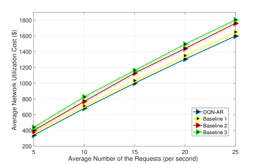
Figure 8: Average network utilization cost versus the average number of requests per second

V-C2 Effect of the coefficient $w_{\text{cost}}$ on AAR

The ANUC is very dependent on the AAR, since when the accepted requests increases, the network utilization cost increases simultaneously. Based on this, we try to maximize the number of accepted requests with respect to the constraints and minimize the utilization cost at the same time. Also, as we denote in (24), we consider the reward function with certain coefficients as $w_{\text{acc}}$ and $w_{\text{cost}}$. Accordingly, the coefficient $w_{\text{cost}}$ determines the priority of cost in each action. As we show in Fig. 9, by increasing the coefficient $w_{\text{cost}}$, the AAR deceases.

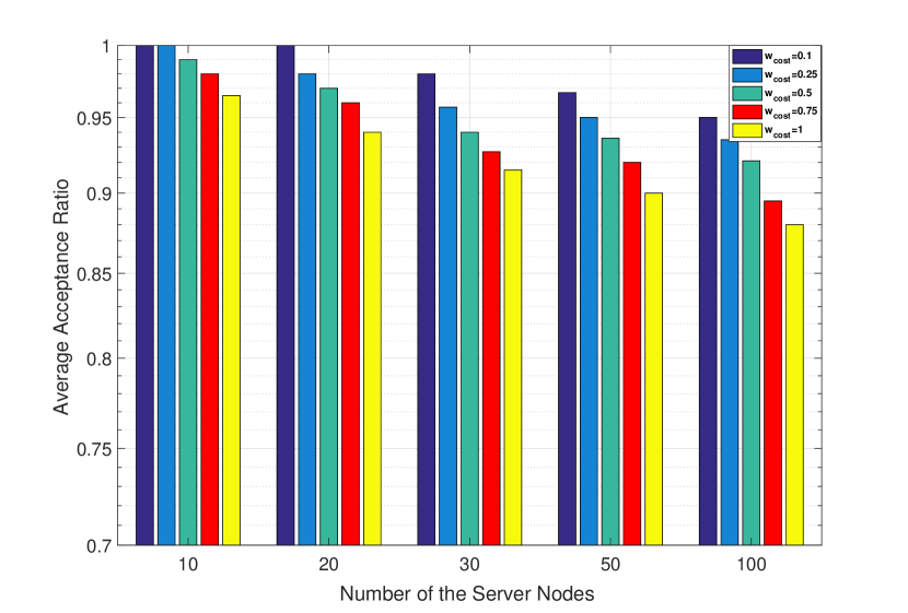
Figure 9: Comparing AAR with considering different coefficient of the cost in reward function

V-C3 Effect of the coefficient $w_{\text{cost}}$ on ANUC

By considering the coefficient $w_{\text{cost}}$, the agent has more attention to minimize the ANUC. Therefore, the agent chooses actions that have less cost, but these actions can not provide sufficient resources for the next requests Fig. 10. Because ANUC is closely dependent on the AAR, by decreasing AAR, ANUC gradually decreases, but by considering this coefficient, AAR decreases 12% and ANUC decreases 20$\%$ in the proposed DQN-AR method. In addition, to evaluate the effect of coefficient $w_{\text{cost}}$ on the baselines, we illustrate the obtained results in Fig. 10. Baseline 1, by placing the VNF in the VMs by the NFVdeep algorithm achieves more ANUC compared to the proposed method. Baseline 2 deploys Tabu-search algorithm for function placement and routing and achieves higher cost than baseline 1. Finally, baseline 3, by deploying greedy-based selection criteria, has the worst results specifically in the case of large networks.

Figure 10: Performance evaluation of the proposed method and the baselines by changing the coefficient $w_{\text{cost}}$

V-C4 Effect of Average Service Life Time on AAR

Average service life is a parameter that depends on the type of services. To evaluate the effect of the service life time on AAR, we consider the service life time with 240 to 1200 seconds. As can be seen in Fig. 12, increasing the services lifetime has more effect on AAR compared to the number of requests. This is because when service lifetime becomes large, the available resource decreases. In addition, by considering the exponential distribution for the users’ service lifetime, after a period of time equal to the mean of exponential distribution from the users’ arrival time, as can be seen in Fig. 11, only 36$\%$ of these users departure the services. Because effective resource allocation according to the service specification have a significant effect on the AAR, DQN-AR by considering network resources and the service specification in the network state can adapt to the conditions that the available resources of network is limited. In addition, DQN-AR by performing an adaptive resource allocation, and dynamic routing achieves better results than baselines.

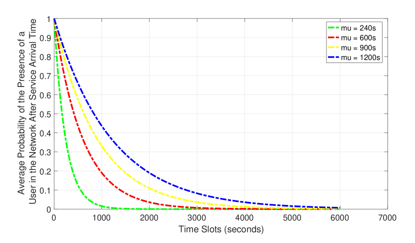
Figure 11: Average probability of the presence of a user in the network after service arrival time.

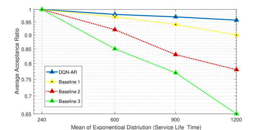
Figure 12: The effect of the service life time on AAR

Figure 13: The effect of the network resources on AAR

V-C5 Effect Network Resources on AAR

To evaluate the effect of the available network resource on AAR, we consider that the users have maximum (1200 seconds) service life time. As can be seen in Fig. 13, by increasing the server nodes and links, the available resources increases and the agent can accept more service requests. Because the proposed DQN-AR algorithm can consider some of the nodes as switch or for function placement and also deploy a dynamic node by node routing, it has higher AAR in different network typologies.

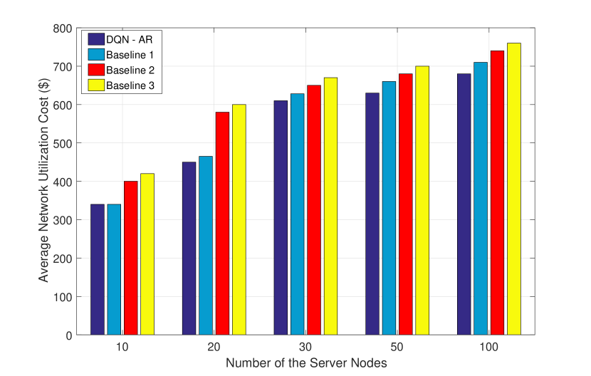
Figure 14: Effect of the network size and number of the server nodes on ANUC

V-C6 Effect of the network topology on ANUC

As we evaluated in Section V-B2, by increasing the network size and the number of the server nodes, because the paths become longer, the AUNC is increased as shown in Fig. 14. In fact, by increasing the server nodes, the network becomes bigger and also more scattered. By solving the routing and function placement jointly in the proposed DQN-AR algorithm, the ANUC is less than that of the other baselines. In summery, since DQN-AR is an online and adaptive algorithm in routing and function placement, it shows good performance in different conditions.

VI Future works

It will be important that future researches investigate the performance of the new RL-based methods that deploy combined methods like Recurrent Deterministic Policy Gradient (RDPG) to provide proactive and predictive resource allocation algorithms in NFV-enabled networks. Therefore, in future works, we will study other RL-algorithms in NFV-enabled networks.

VII Conclusion

We studied an online service provision framework by considering lifetime for each service and using RA approach in a NFV-enabled network. To this end, we formulated the cost of the network resource utilization for function placement and routing of the requested services by considering services requirements and resource constraints. To minimize the resource utilization cost by maximizing the service acceptance ratio, we defined the reward as a piecewise function. Because of the large number of actions and states space, we used a DQN structure. Simulation results show the effectiveness of the proposed model. By evaluating the baselines, the network utilization cost is decreases by $5$ and $20\%$ and average number of admitted request increases by $7$ up to $20$%.

References

- [1] M. Series, “IMT vision–framework and overall objectives of the future development of imt for 2020 and beyond,” Recommendation ITU, pp. 2083–0, Sep. 2015.
- [2] R. Cziva and D. P. Pezaros, “Container network functions: Bringing NFV to the network edge,” IEEE Communications Magazine, vol. 55, no. 6, pp. 24–31, June. 2017.
- [3] J. Pei, P. Hong, and D. Li, “Virtual network function selection and chaining based on deep learning in SDN and NFV-enabled networks,” in Proc. IEEE International Conference on Communications Workshops (ICC Workshops), Kansas City, USA, May. 2018, pp. 1-6.
- [4] Q. Mao, F. Hu, and Q. Hao, “Deep learning for intelligent wireless networks: A comprehensive survey,” IEEE Communications Surveys Tutorials, vol. 20, no. 4, pp. 2595–2621, Jun. 2018.
- [5] J. G. Herrera and J. F. Botero, “Resource allocation in NFV: A comprehensive survey,” IEEE Transactions on Network and Service Management, vol. 13, no. 3, pp. 518–532, August. 2016.
- [6] M. Hamann and M. Fischer, “Path-based optimization of NFV-resource allocation in SDN networks,” in Proc. IEEE International Conference on Communications (ICC), Shanghai, China, July. 2019, pp. 1-6.
- [7] Y. Xiao, Q. Zhang, F. Liu, J. Wang, M. Zhao, Z. Zhang, and J. Zhang, “NFVdeep: Adaptive online service function chain deployment with deep reinforcement learning,” in Proc. International Symposium on Quality of Service (IWQoS), Phoenix, Arizona, USA, June. 2019, pp. 1–10.
- [8] C. Zhang, H. Zhang, J. Qiao, D. Yuan, and M. Zhang, “Deep transfer learning for intelligent cellular traffic prediction based on cross-domain big data,” IEEE Journal on Selected Areas in Communications, vol. 37, no. 6, pp. 1389–1401, March. 2019.
- [9] N. Gholipoor, H. Saeedi, N. Mokari, and E. Jorswieck, “E2E QoS guarantee for the tactile internet via joint NFV and radio resource allocation,” IEEE Transactions on Network and Service Management, June. 2020.
- [10] A. Alleg, T. Ahmed, M. Mosbah, R. Riggio, and R. Boutaba, “Delay-aware VNF placement and chaining based on a flexible resource allocation approach,” in Proc. IEEE International Conference on Network and Service Management (CNSM), Tokyo, Japan, USA, Nov. 2017, pp. 1-7.
- [11] H. Ren, Z. Xu, W. Liang, Q. Xia, P. Zhou, O. F. Rana, A. Galis, and G. Wu, “Efficient algorithms for delay-aware NFV-enabled multicasting in mobile edge clouds with resource sharing,” IEEE Transactions on Parallel and Distributed Systems, March. 2020.
- [12] I. R. D. Kamgang, G. E. M. Zhioua, and N. Tabbane, “A slice-based decentralized NFV framework for an End-to-End QoS-based dynamic resource allocation,” Journal of Ambient Intelligence and Humanized Computing, pp. 1–19, Jan. 2020.
- [13] R. Mijumbi, J. Serrat, J.-L. Gorricho, N. Bouten, F. De Turck, and S. Davy, “Design and evaluation of algorithms for mapping and scheduling of virtual network functions,” in Proc. IEEE Conference on Network Softwarization (NetSoft), London, UK, April. 2015, pp. 1–9.
- [14] T.-H. Nguyen, J. Lee, and M. Yoo, “A practical model for optimal placement of virtual network functions,” in Proc. IEEE International Conference on Information Networking (ICOIN), Kuala Lumpur, Malaysia, May. 2019, pp. 239–241.
- [15] X. Chen, W. Ni, T. Chen, I. B. Collings, X. Wang, R. P. Liu, and G. B. Giannakis, “Multi-timescale online optimization of network function virtualization for service chaining,” IEEE Transactions on Mobile Computing, vol. 18, no. 12, pp. 2899–2912, Dec. 2018.
- [16] Q. Mao, F. Hu, and Q. Hao, “Deep learning for intelligent wireless networks: A comprehensive survey,” IEEE Communications Surveys & Tutorials, vol. 20, no. 4, pp. 2595–2621, 2018.
- [17] J. Li, H. Gao, T. Lv, and Y. Lu, “Deep reinforcement learning based computation offloading and resource allocation for MEC,” in Proc. IEEE Wireless Communications and Networking Conference (WCNC), Barcelona, Spain, June. 2018, pp. 1–6.
- [18] S. Ayoubi, N. Limam, M. A. Salahuddin, N. Shahriar, R. Boutaba, F. Estrada-Solano, and O. M. Caicedo, “Machine learning for cognitive network management,” IEEE Communications Magazine, vol. 56, no. 1, pp. 158–165, Jan. 2018.
- [19] L. M. M. Zorello, M. G. T. Vieira, R. A. G. Tejos, M. A. T. Rojas, C. Meirosu, and T. C. M. de Brito Carvalho, “Improving energy efficiency in NFV clouds with machine learning,” in Proc. IIEEE International Conference on Cloud Computing (CLOUD), San Francisco, CA, USA, July. 2018, pp. 710–717.
- [20] R. Ding, Y. Xu, F. Gao, X. Shen, and W. Wu, “Deep reinforcement learning for router selection in network with heavy traffic,” IEEE Access, vol. 7, pp. 37109–37120, March. 2019.
- [21] J. Pei, P. Hong, and D. Li, “Virtual network function selection and chaining based on deep learning in SDN and NFV-enabled networks,” in Proc. IEEE International Conference on Communications Workshops (ICC Workshops), Kansas City, MO, USA, July. 2018, pp. 1–6.
- [22] J. Zhou, P. Hong, and J. Pei, “Multi-task deep learning based dynamic service function chains routing in SDN/NFV-enabled networks,” in Proc. IEEE International Conference on Communications (ICC), Shanghai, China, May. 2019, pp. 1–6.
- [23] T. ZSubramanya and R. Riggio, “Machine learning-driven scaling and placement of virtual network functions at the network edges,” in Proc. IEEE International Conference on Network Softwarization (NetSoft), Paris, France, Aug. 2019, pp. 414–422.
- [24] B. Wu, J. Zeng, L. Ge, S. Shao, Y. Tang, and X. Su, “Resource allocation optimization in the NFV-enabled MEC network based on game theory,” in Proc. IEEE International Conference on Communications (ICC), Shanghai, China, July. 2019, pp. 1–7.
- [25] X. Fu, F. R. Yu, J. Wang, Q. Qi, and J. Liao, “Dynamic service function chain embedding for NFV-enabled IoT: A deep reinforcement learning approach,” IEEE Transactions on Wireless Communications, Oct. 2019.
- [26] C. Pham, N. H. Tran, and C. S. Hong, “Virtual network function scheduling: A matching game approach,” IEEE Communications Letters, vol. 22, no. 1, pp. 69–72, Aug. 2017.
- [27] M. Li, Q. Zhang, and F. Liu, “Finedge: A dynamic cost-efficient edge resource management platform for NFV network,” in Proc. IEEE/ACM International Symposium on Quality of Service (IWQoS), Hang Zhou, China, Oct. 2020, pp. 1–10.
- [28] Z. Ning, N. Wang, and R. Tafazolli, “Deep reinforcement learning for NFV-based Service Function Chaining in Multi-Service Networks,” in Proc. IEEE International Conference on High Performance Switching and Routing (HPSR), Newark, NJ, USA, May. 2020, pp. 1–6.
- [29] J. Pei, P. Hong, M. Pan, J. Liu, and J. Zhou, “Optimal VNF placement via deep reinforcement learning in SDN/NFV-enabled networks,” IEEE Journal on Selected Areas in Communications, vol. 38, no. 2, pp. 263–278, Dec. 2019.
- [30] K. Qu, W. Zhuang, Q. Ye, X. Shen, X. Li, and J. Rao, “Dynamic flow migration for embedded services in SDN/NFV-enabled 5G core networks,” IEEE Transactions on Communications, vol. 68, no. 4, pp. 2394–2408, Jan. 2020.
- [31] Y. Jia, C. Wu, Z. Li, F. Le, and A. Liu, “Online scaling of NFV service chains across geo-distributed datacenters,” IEEE/ACM Transactions on Networking, vol. 26, no. 2, pp. 699–710, 2018.
- [32] M. Huang, W. Liang, Y. Ma, and S. Guo, “Maximizing throughput of delay-sensitive NFV-enabled request admissions via virtualized network function placement,” IEEE Transactions on Cloud Computing, 2019.
- [33] Z. Xu, W. Liang, A. Galis, Y. Ma, Q. Xia, and W. Xu, “Throughput optimization for admitting NFV-enabled requests in cloud networks,” Computer Networks, vol. 143, pp. 15–29, 2018.
- [34] 3GPP, TS 28.530, “Technical specification group services and system aspects; management and orchestration; Concepts, use cases and requirements,” Sep. 2019.
- [35] N. ETSI, “GS NFV-MAN 001 v1. 1.1 network functions virtualisation (NFV); management and orchestration,” tech. rep., Dec. 2014.
- [36] P. Hong, K. Xue, D. Li, et al., “Resource aware routing for service function chains in SDN and NFV-enabled network,” IEEE Transactions on Services Computing, June. 2018.
- [37] M. Savi, M. Tornatore, and G. Verticale, “Impact of processing-resource sharing on the placement of chained virtual network functions,” IEEE Transactions on Cloud Computing, May. 2019.
- [38] G. Liu, Y. Ren, M. Yurchenko, K. Ramakrishnan, and T. Wood, “Microboxes: high performance NFV with customizable, asynchronous TCP stacks and dynamic subscriptions,” in Proc. Conference of the ACM Special Interest Group on Data Communication (SIGCOMM), Budapest Hungary, Aug. 2018, pp. 504–517.
- [39] M. M. Tajiki, S. Salsano, L. Chiaraviglio, M. Shojafar, and B. Akbari, “Joint energy efficient and QoS-aware path allocation and VNF placement for service function chaining,” IEEE Transactions on Network and Service Management, vol. 16, no. 1, pp. 374–388, Oct. 2018.
- [40] S. Ebrahimi, A. Zakeri, B. Akbari, and N. Mokari, “Joint resource and admission management for slice-enabled networks,” in Proc. EEE/IFIP Network Operations and Management Symposium (NOMS), Budapest, Hungary, June. 2020, pp. 1–7.
- [41] G. Miotto, M. C. Luizelli, W. L. da Costa Cordeiro, and L. P. Gaspary, “Adaptive placement & chaining of virtual network functions with NFV,” Journal of Internet Services and Applications, vol. 10, no. 1, pp. 1–19, Feb. 2019.
- [42] R. S. Sutton and A. G. Barto, Reinforcement learning: An introduction. MIT press, 2018.
- [43] M. Tokic and G. Palm, “Value-difference based exploration: adaptive control between epsilon-greedy and softmax,” in Annual conference on artificial intelligence, pp. 335–346, Springer, 2011.
- [44] H. Van Hasselt and M. A. Wiering, “Reinforcement learning in continuous action spaces,” in 2007 IEEE International Symposium on Approximate Dynamic Programming and Reinforcement Learning, pp. 272–279, IEEE, 2007.
- [45] A. Leivadeas, G. Kesidis, M. Ibnkahla, and I. Lambadaris, “VNF placement optimization at the edge and cloud,” Future Internet, vol. 11, no. 3, p. 69, March. 2019.
- [46] S. Sheikhzadeh, M. Pourghasemian, M. R. Javan, N. Mokari, and E. A. Jorswieck, “AI-based secure NOMA and cognitive radio enabled green communications: Channel state information and battery value uncertainties,” arXiv preprint arXiv:2106.15964, 2021.
- [47] Y. Li, L. Gao, S. Xu, Q. Ou, X. Yuan, F. Qi, S. Guo, and X. Qiu, “Cost-and-QoS-based NFV service function chain mapping mechanism,” in NOMS 2020-2020 IEEE/IFIP Network Operations and Management Symposium, pp. 1–9, IEEE, 2020.
- [48] S. Agarwal, F. Malandrino, C.-F. Chiasserini, and S. De, “Joint VNF placement and CPU allocation in 5G,” in Proc. IEEE INFOCOM Conference on Computer Communications, Honolulu, HI, USA, Oct. 2018, pp. 1943–1951.
- [49] A. Nouruzi, “Code of NFV Paper, DOI: https://dx.doi.org/10.21227/r1j8-tc84, https://ieee-dataport.org/documents/anazmrjnm2021files,”