Deep Least Squares Alignment for Unsupervised Domain Adaptation

Abstract

Unsupervised domain adaptation leverages rich information from a labeled source domain to model an unlabeled target domain. Existing methods attempt to align the cross-domain distributions. However, the statistical representations of the alignment of the two domains are not well addressed. In this paper, we propose deep least squares alignment (DLSA) to estimate the distribution of the two domains in a latent space by parameterizing a linear model. We further develop marginal and conditional adaptation loss to reduce the domain discrepancy by minimizing the angle between fitting lines and intercept differences and further learning domain invariant features. Extensive experiments demonstrate that the proposed DLSA model is effective in aligning domain distributions and outperforms state-of-the-art methods.

1 Introduction

Large amounts of labeled data is a prerequisite to training accurate predictors in most machine learning techniques. However, manually labeling and training a model from scratch is tedious and expensive. Fortunately, unsupervised domain adaptation (UDA) aims to deal with the shortage of labels by leveraging a richly labeled source domain to a similar but different unlabeled target domain. This task is usually challenged by the dataset bias or domain shift issue because source and target domains have different characteristics. UDA can mitigate this by establishing the association between domains and learning domain invariant features.

Recent advances in UDA witness its success in deep neural networks. It can learn abstract representations with nonlinear transformations and suppress the negative effects caused by the domain shift. In earlier work, deep learning based methods rely on minimizing the discrepancy between the source and target distributions by proposing different loss functions, such as Maximum Mean Discrepancy (MMD) [Tzeng et al.(2014)Tzeng, Hoffman, Zhang, Saenko, and Darrell], CORrelation ALignment (CORAL) [Sun and Saenko(2016)], Kullback-Leibler divergence (KL) [Meng et al.(2018)Meng, Li, Gong, and Juang]. Inspired by generative adversarial network (GAN)  [Goodfellow et al.(2014)Goodfellow, Pouget-Abadie, Mirza, Xu, Warde-Farley, Ozair, Courville, and Bengio], adversarial domain adaptation methods aim to identify domain invariant features by playing a min-max game between domain discriminator and feature extractor [Ghifary et al.(2014)Ghifary, Kleijn, and Zhang, Tzeng et al.(2017)Tzeng, Hoffman, Saenko, and Darrell, Zhang and Davison(2020a), Zhang and Davison(2021b), Zhang and Davison(2020b)]. However, these methods either cannot fully align the marginal and conditional distributions between two domains or request additional components such as a domain discriminator [Tzeng et al.(2017)Tzeng, Hoffman, Saenko, and Darrell] or gradient reversal layer [Ghifary et al.(2014)Ghifary, Kleijn, and Zhang].

Although many methods achieve remarkable results in domain adaptation, they still suffer from two challenges: 1) the distributions of two domains cannot be intuitively represented, and alignment processes are hidden; and, 2) the label information and latent structure of the target domain are not fully considered, and how to better align marginal and conditional distributions are not well addressed. To alleviate these challenges, we propose a deep least squares adaptation (DLSA) model with a toy example shown in Fig. 1.

We offer two contributions:

1. We propose a simple and novel UDA approach, DLSA, to explicitly model the distribution of domains in the latent space with estimated fitting lines, which are parameterized by estimated slope and intercept. We further theoretically and statistically show the effectiveness of DLSA in estimating domain distributions.

2. We design and effectively integrate marginal and conditional adaptation losses to impose distribution alignment. By minimizing angle and intercept differences between source and target fitting lines, we enforce feature discriminability, which leads to inter-class dispersion and intra-class compactness.

Experimental results on three benchmark datasets show that DLSA achieves higher classification performance than state-of-the-art methods. We also statistically show the estimated least squares parameters to model the distributions of source and target domains.

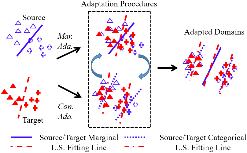
Figure 1: Schematic diagram of the proposed least squares alignment. We first estimate the least squares fitting lines of two domains and then align the marginal and conditional distributions. By rotating and translating the fitting lines, the distributions between the two domains can be aligned, and domain discrepancy is minimized (Mar.: marginal, Con.: conditional, and Ada.: adaptation).

2 Related work

There are different deep techniques for UDA. To learn domain invariant representations, early methods attempt to propose distance-based loss functions to align data distributions between different domains. Maximum Mean Discrepancy (MMD) [Tzeng et al.(2014)Tzeng, Hoffman, Zhang, Saenko, and Darrell] is one of the most popular distance functions to minimize between two distributions. Deep Adaptation Network (DAN) considered the sum of MMD from several layers with multiple kernels of MMD functions [Long et al.(2015)Long, Cao, Wang, and Jordan]. The CORAL loss is another distance function, based on covariance matrices of the latent features from two domains [Sun and Saenko(2016)]. Recently, Li et al. [Li et al.(2020a)Li, Zhai, Luo, Ge, and Ren] proposed an Enhanced Transport Distance (ETD) to measure domain discrepancy by establishing the transport distance of attention perception as the predictive feedback of iterative learning classifiers.

With the advent of GAN [Goodfellow et al.(2014)Goodfellow, Pouget-Abadie, Mirza, Xu, Warde-Farley, Ozair, Courville, and Bengio], adversarial learning models have been found to be an impactful mechanism for identifying invariant representations in domain adaptation and minimizing the domain discrepancy. The Domain Adversarial Neural Network (DANN) considered a minimax loss to integrate a gradient reversal layer to promote the discrimination of source and target domains [Ganin et al.(2016)Ganin, Ustinova, Ajakan, Germain, Larochelle, Laviolette, Marchand, and Lempitsky]. The Adversarial Discriminative Domain Adaptation (ADDA) method utilized an inverted labeled GAN loss to split the source and target domains, and features can be learned separately [Tzeng et al.(2017)Tzeng, Hoffman, Saenko, and Darrell]. Xu et al. ([Xu et al.(2019)Xu, Zhang, Ni, Li, Wang, Tian, and Zhang]) mapped the two domains to a common potential distribution and effectively transfers domain knowledge. There are also many methods that utilized pseudo-labels to consider label information in the target domain [Chen et al.(2019)Chen, Xie, Huang, Rong, Ding, Huang, Xu, and Huang, Kang et al.(2019)Kang, Jiang, Yang, and Hauptmann, Zhang et al.(2021)Zhang, Ye, and Davison]. They have not, however, intuitively studied the distribution adaptation as thoroughly as we do in Fig. 3 of supplemental material.

Least squares estimation is also used in domain adaptation, but most are proposed to solve regression problems. Huang et al. [Huang et al.(2020)Huang, Chen, Li, Chen, Yuan, and Shi] proposed a domain adaptive partial least squares regression model, which utilized the Hilbert-Schmidt independence criterion to estimate the independence of the extracted latent variables and domain labels. The partial least squares method was used to align the source and target data in the latent space via estimating a projection matrix. Similarly, Nikzad-Langerodi et al. [Nikzad-Langerodi et al.(2020)Nikzad-Langerodi, Zellinger, Saminger-Platz, and Moser] considered UDA for regression problems under Beer–Lambert’s law. They employed a non-linear iterative partial least squares algorithm to minimize the covariance matrices difference of the latent sample between two domains. Yuan et al. [Yuan et al.(2020)Yuan, Li, Zhu, Li, and Gu] proposed to use least squares distance to align marginal distribution between two domains for classification problem. However, the so-called least-squares distance is proposed by Mao et al. [Mao et al.(2017)Mao, Li, Xie, Lau, Wang, and Paul Smolley], aiming to push generated samples toward the decision boundary and reduce the gradient vanishing problem during adversarial learning. Notably, we focus on UDA for visual recognition and impose marginal and conditional distribution adaptation losses based on slope and intercept differences from the least squares estimation.

3 Methodology

3.1 Problem and motivation

For unsupervised domain adaptation, given a source domain $\mathcal{D_{S}}=\{\mathcal{X}_{\mathcal{S}}^{i},\mathcal{Y}_{\mathcal{S}}^{i}\}_{i=1}^{\mathcal{N}_{\mathcal{S}}}$ of $\mathcal{N}_{\mathcal{S}}$ labeled samples in $C$ categories and a target domain $\mathcal{D_{T}}=\{\mathcal{X}_{\mathcal{T}}^{j}\}_{j=1}^{\mathcal{N}_{\mathcal{T}}}$ of $\mathcal{N}_{\mathcal{T}}$ samples without any labels (i.e., $\mathcal{Y}_{\mathcal{T}}$ is unknown). Our ultimate goal is to learn a classifier $\mathcal{F}$ under a feature extractor $G$, which reduces domain discrepancy and improves the generalization ability of the classifier to the target domain.

To achieve it, existing methods usually attempt to align either marginal or conditional distributions of the two domains. Moreover, the statistical estimation of distributions is not well addressed. In contrast, we propose to align both distributions to further reduce domain discrepancies. In particular, we employ least squares to estimate the latent space distribution, which is parameterized by a slope and an intercept. We then design marginal and conditional adaptation losses to enforce the distribution alignment both in inter-class and intra-class. In turn, we can push the decision boundary of classifier $\mathcal{F}$ toward the target domain.

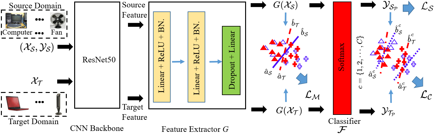
Figure 2: The architecture of our proposed DLSA model. We first employ a ResNet50-based feature extractor $G$ to acquire the feature representations of two domains. DLSA consists of three loss functions (classification loss $\mathcal{L_{S}}$, marginal adaptation loss $\mathcal{L_{M}}$, and conditional adaptation loss $\mathcal{L_{C}}$). The marginal distribution is aligned via reducing the global angle and intercept differences between source and target fitting lines. The conditional distribution is aligned by categorical angle and intercept differences of two domains (BN.: BatchNormalization).

3.2 Source Classifier

For the labeled source domain, we minimize the following classification loss:

$$\mathcal{L_{S}}=J(\mathcal{F}(G(\mathcal{X}_{\mathcal{S}})),\mathcal{Y_{S}}),$$ (1)

where $\mathcal{F}$ is the classifier, $J(\cdot,\cdot)$ is the cross-entropy loss and $\mathcal{Y_{S_{P}}}=\mathcal{F}(G(\mathcal{X}_{\mathcal{S}}))$ is the predicted label in Fig. 2.

3.3 Least squares estimation

The feature extractor $G$ maps samples from a given neural network layer into a $d$-dimensional latent space ($d>1$). The latent source and target samples can be denoted as: $G(\mathcal{X_{S}})\in\mathbb{R}^{\mathcal{N_{S}}\times d}$, and $G(\mathcal{X_{T}})\in\mathbb{R}^{\mathcal{N_{T}}\times d}$, respectively. Next, we aim to model domain distribution via estimating the fitting line of two domains in the latent space, which has the minimum error to all latent samples. The latent samples can be encoded via $G(\mathcal{X_{Z}})=[G(\mathcal{X_{Z}})^{1},G(\mathcal{X_{Z}})^{d-1}]$, where $\mathcal{Z}$ can be either source domain $\mathcal{S}$ or target domain $\mathcal{T}$. Let $L_{V}^{\mathcal{Z}}=G(\mathcal{X_{Z}})^{1}\in\mathbb{R}^{\mathcal{N_{Z}}\times 1}$ and $L_{W}^{\mathcal{Z}}=G(\mathcal{X_{Z}})^{d-1}\in\mathbb{R}^{\mathcal{N_{Z}}\times(d-1)}$, $L_{V}^{z}$ and $L_{W}^{z}$ are each one of the elements, respectively, i.e., $L_{V}^{z}\in\mathbb{R}$, which is a scalar and $L_{W}^{z}\in\mathbb{R}^{d-1}(z=1,2,\cdots,\mathcal{N_{Z}})$. To model the distribution of latent space, we naively assume that there is a linear relationship between $L_{V}^{\mathcal{Z}}$ and $L_{W}^{\mathcal{Z}}$. The motivation is that we aim to use the slope and intercept to represent the distribution of the latent feature $G(\mathcal{X_{Z}})$. Then, we can minimize the difference of slope and intercept of the two domains. Moreover, such a linear fitting line can always be estimated (except when there is only one sample for estimation). Here, we arbitrarily choose the first dimension as the independent variable, and the remaining $d-1$ dimensions as dependent variables; other dimensions are explored in supplemental material.

Before formulating distribution alignment, we first review multiple linear regression in $\mathbb{R}^{d-1}$. Given the target variable (dependent variable) $L_{W}^{\mathcal{Z}}$ taking values in $\mathbb{R}^{d-1}$, and independent variable $L_{V}^{\mathcal{Z}}$ taking values in $\mathbb{R}$, the multiple linear regression model is given by:

$$L_{W}^{\mathcal{Z}}=a_{\mathcal{Z}}L_{V}^{\mathcal{Z}}+b_{\mathcal{Z}}+\epsilon,$$ (2)

where $a_{\mathcal{Z}}\in\mathbb{R}^{d-1}$ contains the unobservable slope parameter, $b_{\mathcal{Z}}\in\mathbb{R}^{d-1}$ holds unobservable intercept parameter, and $\epsilon$ is unobservable random noise, which is drawn i.i.d.

Consider a data set of input $L_{V}^{\mathcal{Z}}=\{L_{V}^{z}\}_{z=1}^{\mathcal{N_{Z}}}$ with corresponding target value $L_{W}^{\mathcal{Z}}=\{L_{W}^{z}\}_{z=1}^{\mathcal{N_{Z}}}$, the least squares estimate of the slope $\hat{a}_{\mathcal{Z}}$ and intercept $\hat{b}_{\mathcal{Z}}$ via solving the minimization problem in Eq. 3.

$$\hat{a}_{\mathcal{Z}},\hat{b}_{\mathcal{Z}}=\arg\min\sum_{z=1}^{\mathcal{N_{Z}}}||L_{W}^{z}-a_{\mathcal{Z}}L_{V}^{z}-b_{\mathcal{Z}}||^{2}$$ (3)

Let $E=\sum_{z=1}^{\mathcal{N_{Z}}}||L_{W}^{z}-a_{\mathcal{Z}}L_{V}^{z}-b_{\mathcal{Z}}||^{2}$, to estimate coefficients, we take the gradient of $E$ with respect to each parameter, and setting the result equal to zero.

$$\frac{\partial E}{\partial a_{\mathcal{Z}}}=-2\sum_{z=1}^{\mathcal{N_{Z}}}L_{V}^{z}(L_{W}^{z}-a_{\mathcal{Z}}L_{V}^{z}-b_{\mathcal{Z}})=0,\quad\frac{\partial E}{\partial b_{\mathcal{Z}}}=-2\sum_{z=1}^{\mathcal{N_{Z}}}(L_{W}^{z}-a_{\mathcal{Z}}L_{V}^{z}-b_{\mathcal{Z}})=0$$ (4)

The estimation of the true parameters are denoted by $\hat{a}_{\mathcal{Z}}$ and $\hat{b}_{\mathcal{Z}}$, solving Eq. LABEL:eq:par, we can get

$$\hat{a}_{\mathcal{Z}}=\frac{\frac{1}{\mathcal{N_{Z}}}\sum_{z=1}^{\mathcal{N_{Z}}}L_{V}^{z}L_{W}^{z}-\mkern 3.5mu\overline{\mkern-3.5muL_{V}^{\mathcal{Z}}\mkern-3.5mu}\mkern 3.5mu\mkern 3.5mu\overline{\mkern-3.5muL_{W}^{\mathcal{Z}}\mkern-3.5mu}\mkern 3.5mu}{\frac{1}{\mathcal{N_{Z}}}\sum_{z=1}^{\mathcal{N_{Z}}}L_{V}^{z}-\mkern 3.5mu\overline{\mkern-3.5muL_{V}^{\mathcal{Z}}\mkern-3.5mu}\mkern 3.5mu^{2}},\quad\quad\hat{b}_{\mathcal{Z}}=\mkern 3.5mu\overline{\mkern-3.5muL_{W}^{\mathcal{Z}}\mkern-3.5mu}\mkern 3.5mu-\hat{a}_{\mathcal{Z}}\mkern 3.5mu\overline{\mkern-3.5muL_{V}^{\mathcal{Z}}\mkern-3.5mu}\mkern 3.5mu$$ (5)

where $\mathcal{Z}$ can be either $\mathcal{S}$ or $\mathcal{T}$, $\mkern 3.5mu\overline{\mkern-3.5muL_{V}^{\mathcal{Z}}\mkern-3.5mu}\mkern 3.5mu$ and $\mkern 3.5mu\overline{\mkern-3.5muL_{W}^{\mathcal{Z}}\mkern-3.5mu}\mkern 3.5mu$ are the mean of $L_{V}^{\mathcal{Z}}$ and $L_{W}^{\mathcal{Z}}$, respectively. Therefore, we are able to model the fitting lines of two domains via $L_{W}^{\mathcal{S}}=\hat{a}_{\mathcal{S}}L_{V}^{\mathcal{S}}+\hat{b}_{\mathcal{S}}$ and $L_{W}^{\mathcal{T}}=\hat{a}_{\mathcal{T}}L_{V}^{\mathcal{T}}+\hat{b}_{\mathcal{T}}$. In the following section, we present the distribution alignment with the estimated key coefficients $(\hat{a}_{\mathcal{S}},\hat{b}_{\mathcal{S}},\hat{a}_{\mathcal{T}},\hat{b}_{\mathcal{T}})$, which are the slope and intercept of the source and the target domain, respectively.

3.3.1 Marginal adaptation loss

Before the alignment process, the marginal distribution of the two domains may partially overlap. To learn a separable geometric structure of marginal or global distribution, we consider the estimated parameters of two domains. It can be reached via maximizing the similarities between slope and intercept of two domains, which can be achieved by minimizing the following loss function:

$$\mathcal{L_{M}}=||\hat{a}_{\mathcal{S}}-\hat{a}_{\mathcal{T}}||_{F}^{2}+\gamma||\hat{b}_{\mathcal{S}}-\hat{b}_{\mathcal{T}}||_{F}^{2},$$ (6)

where $\mathcal{M}$ denotes marginal distribution, $||\cdot||_{F}$ is the Frobenius norm and $\gamma$ balances the scale between two terms. The first term enforces small differences of slope between two domains, which is equivalent to minimizing the marginal/global angle ($\theta_{\mathcal{M}}$) between two fitting lines as in Eq. 7.

$$\theta_{\mathcal{M}}=\arccos{\frac{\hat{a}_{\mathcal{S}}\cdot\hat{a}_{\mathcal{T}}}{|\hat{a}_{\mathcal{S}}|\cdot|\hat{a}_{\mathcal{T}}|}}$$ (7)

We can reformulate Eq. 6 as follows:

$$\mathcal{L_{M}}=\theta_{\mathcal{M}}+\gamma\mathcal{B}_{\mathcal{M}},$$ (8)

where $\mathcal{B}_{\mathcal{M}}=||\hat{b}_{\mathcal{S}}-\hat{b}_{\mathcal{T}}||_{F}^{2}$ represents the marginal intercept difference between two domains. The marginal adaptation loss in Eq. 8 first minimizing the angle of the two fitting lines, which is similar to rotating two fitting lines and leads to the same slope. It then minimizes the estimated intercepts of the two lines, which is equivalent to translating $\hat{b}_{\mathcal{S}}$ to $\hat{b}_{\mathcal{T}}$. As shown in Fig. 2, there is a 2-dimensional space with 2 classes. Let $\{1,2\}$ be the labels of “triangle" and “cross". According to the goal of Eq. 8, the marginal distribution alignment of the two domains can be achieved by finding a minimal $\theta_{\mathcal{M}}$ and intercept difference $\mathcal{B}_{\mathcal{M}}$.

3.3.2 Conditional adaptation loss

Eq. 8 can only minimize the marginal distribution divergences between the two domains. The conditional distributions are not aligned. Therefore, we need to design a conditional adaptation loss to minimize the conditional distribution divergences between the two domains. Since there are no labels in the target domain, the conditional distribution alignment is facilitated by soft pseudo-labels for the target domain. Given the trained classifier $\mathcal{F}$ in Eq. 1, we can get the dominant predicted class for each target sample as $\mathcal{Y}_{\mathcal{T_{P}}}^{j}=\text{argmax}\ \mathcal{F}(G(\mathcal{X}_{\mathcal{T}}^{j}))$. We hence get the label information for the latent target samples $G(\mathcal{X}_{\mathcal{T}})$ and these soft pseudo-labels can be refined via minimizing Eq. 1 and Eq. 8. To estimate the categorical slope and intercept, we modified Eq. LABEL:eq:parae as:

$$\hat{a}_{\mathcal{Z}}^{c}=\frac{\frac{1}{\mathcal{N}_{\mathcal{Z}}^{c}}\sum_{z=1}^{\mathcal{N}_{\mathcal{Z}}^{c}}L_{V}^{z}L_{W}^{z}-\mkern 3.5mu\overline{\mkern-3.5muL_{V}^{\mathcal{Z}^{c}}\mkern-3.5mu}\mkern 3.5mu\mkern 3.5mu\overline{\mkern-3.5muL_{W}^{\mathcal{Z}^{c}}\mkern-3.5mu}\mkern 3.5mu}{\frac{1}{\mathcal{N}_{\mathcal{Z}}^{c}}\sum_{z=1}^{\mathcal{N}_{\mathcal{Z}}^{c}}L_{V}^{z}-\mkern 3.5mu\overline{\mkern-3.5muL_{V}^{\mathcal{Z}^{c}}\mkern-3.5mu}\mkern 3.5mu^{2}}\quad\quad\hat{b}_{\mathcal{Z}}^{c}=\mkern 3.5mu\overline{\mkern-3.5muL_{W}^{\mathcal{Z}^{c}}\mkern-3.5mu}\mkern 3.5mu-\hat{a}_{\mathcal{Z}}^{c}\mkern 3.5mu\overline{\mkern-3.5muL_{V}^{\mathcal{Z}^{c}}\mkern-3.5mu}\mkern 3.5mu$$ (9)

where $\mathcal{Z}$ can be either $\mathcal{S}$ or $\mathcal{T}$, $\mathcal{N}_{\mathcal{Z}}^{c}$ is number of samples in each class $c$. $\mkern 3.5mu\overline{\mkern-3.5muL_{V}^{\mathcal{Z}^{c}}\mkern-3.5mu}\mkern 3.5mu$ and $\mkern 3.5mu\overline{\mkern-3.5muL_{W}^{\mathcal{Z}^{c}}\mkern-3.5mu}\mkern 3.5mu$ are the mean of $L_{V}^{\mathcal{Z}^{c}}$ and $L_{W}^{\mathcal{Z}^{c}}$ of class $c$. $L_{V}^{z}$ and $L_{W}^{z}$ naturally become one of the elements of $L_{V}^{\mathcal{Z}^{c}}$ and $L_{W}^{\mathcal{Z}^{c}}$. Therefore, we are able to model the categorical fitting lines of two domains with $L_{W}^{\mathcal{S}^{c}}=\hat{a}_{\mathcal{S}}^{c}L_{V}^{\mathcal{S}^{c}}+\hat{b}_{\mathcal{S}}^{c}$ and $L_{W}^{\mathcal{T}^{c}}=\hat{a}_{\mathcal{T}}^{c}L_{V}^{\mathcal{T}^{c}}+\hat{b}_{\mathcal{T}}^{c}$. Similar to Eq. 6, the conditional adaptation loss is formulated as:

$$\mathcal{L_{C}}=\frac{1}{C}\sum_{c=1}^{C}||\hat{a}_{\mathcal{S}}^{c}-\hat{a}_{\mathcal{T}}^{c}||_{F}^{2}+\gamma\frac{1}{C}\sum_{c=1}^{C}||\hat{b}_{\mathcal{S}}^{c}-\hat{b}_{\mathcal{T}}^{c}||_{F}^{2}.$$ (10)

Specifically, the estimated categorical slope and intercept are based on predicted pseudo-labels. Intuitively, the first term can also be regarded as minimizing the categorical angle $\theta_{\mathcal{C}}^{c}$ between fitting lines as follows.

$$\theta_{\mathcal{C}}^{c}=\arccos{\frac{\hat{a}_{\mathcal{S}}^{c}\cdot\hat{a}_{\mathcal{T}}^{c}}{|\hat{a}_{\mathcal{S}}^{c}|\cdot|\hat{a}_{\mathcal{T}}^{c}|}}$$ (11)

Hence, we can rewrite Eq. 10 as:

$$\mathcal{L_{C}}=\frac{1}{C}\sum_{c=1}^{C}(\theta_{\mathcal{C}}^{c}+\gamma\mathcal{B}_{\mathcal{C}}^{c}),$$ (12)

where $\mathcal{B}_{\mathcal{C}}^{c}=||\hat{b}_{\mathcal{S}}^{c}-\hat{b}_{\mathcal{T}}^{c}||_{F}^{2}$ denotes the conditional intercept difference between two domains of each class $c$. Therefore, the conditional adaptation loss considers each class, and minimizes categorical angle and intercept differences; it is naturally similar to performing categorical fitting line rotation and translation. As shown in Fig. 2, let $\theta_{\mathcal{C}}^{1}$ be the estimated angle between source and target fitting lines of “triangle", and $\theta_{\mathcal{C}}^{2}$ be the estimated angle of “cross". According to Eq. 12, the conditional distribution alignment of the two domains can be achieved by seeking minimal $\theta_{\mathcal{C}}^{1},\theta_{\mathcal{C}}^{2}$ and intercept difference ($\mathcal{B}_{\mathcal{C}}^{1}=||\hat{b}_{\mathcal{S}}^{1}-\hat{b}_{\mathcal{T}}^{1}||,\mathcal{B}_{\mathcal{C}}^{2}=||\hat{b}_{\mathcal{S}}^{2}-\hat{b}_{\mathcal{T}}^{2}||$).

3.4 Overall objective function

We integrate all components and obtain the following overall objective function of DLSA as:

$$\mathcal{L}=\operatorname*{arg\,min}\ (\mathcal{L_{S}}+(1-\alpha)\mathcal{L_{M}}+\alpha\mathcal{L_{C}}),$$ (13)

where $\mathcal{L_{S}}$ is the cross-entropy loss of the classifier in the labeled source domain. $\mathcal{L_{M}}$ and $\mathcal{L_{C}}$ represent the marginal and conditional adaptation loss, respectively. $\alpha$ is the penalty parameter to balance conditional and marginal distribution.

The overall training procedure is straightforward. We first train the labeled source domain and unlabeled target domain using Eqs. 1 and 8 to reduce the marginal distribution discrepancy between two domains. We then generate pseudo-labels ($\mathcal{Y_{T_{P}}}$) for the target domain with the trained classifier $\mathcal{F}$, and minimize the conditional adaptation loss using Eq. 12. Finally, we repeat the previous two steps until the loss function in Eq. 13 has converged.

4 Experiments

4.1 Datasets

Office + Caltech-10 [Gong et al.(2012)Gong, Shi, Sha, and Grauman] has 2,533 images in four domains: Amazon (A), Webcam (W), DSLR (D), and Caltech (C) from ten classes. In experiments, A$\shortrightarrow$W represents transferring knowledge from domain A to domain W. We evaluate twelve tasks in this dataset. Office-31 [Saenko et al.(2010)Saenko, Kulis, Fritz, and Darrell] has 4,110 images from three domains: Amazon (A), Webcam (W), and DSLR (D) in 31 classes. We try six tasks in the Office-31 dataset. The Office-Home [Venkateswara et al.(2017)Venkateswara, Eusebio, Chakraborty, and Panchanathan] dataset contains 15,588 images from four domains: Art (Ar), Clipart (Cl), Product (Pr) and Real-World (Rw) in 65 classes. We also test twelve tasks in this dataset. VisDA-2017 [Peng et al.(2017)Peng, Usman, Kaushik, Hoffman, Wang, and Saenko] is a particularly challenging dataset due to a large domain-shift between the synthetic images (152,397 images from VisDA) and the real images (55,388 images from COCO) in 12 classes. We test our model on the setting of synthetic-to-real as the source-to-target domain and report the accuracy of each category.

4.2 Implementation details

We implement our approach using PyTorch with an Nvidia GeForce 1080 Ti GPU and extract features for the three datasets from a fine-tuned ResNet50 network [He et al.(2016)He, Zhang, Ren, and Sun], which is a neural network well trained on the Imagenet dataset [Krizhevsky et al.(2012)Krizhevsky, Sutskever, and Hinton]. The 1,000 features are then extracted from the last fully connected layer for the source and target features [Zhang and Davison(2019), Zhang and Davison(2020d), Zhang and Davison(2020c)]. In the feature extractor $G$, the outputs of the first two Linear layers are 512, and the output of the last Linear layer is the number of classes in each dataset. The learning rate = 0.001, batch size = 32 and number of iterations = 300.

During training, to balance the scale between slope and intercept, we return the value of angle $\theta_{\mathcal{M}}$ and $\theta_{\mathcal{C}}^{c}$ in radians, which is in the range of $[0,\pi]$. The optimal parameters are $\alpha=0.2$, and $\gamma=0.1$, and $\alpha\in\{0.1,0.2,\cdots,0.9\}$, while $\gamma$ is selected from $\{0.1,0.2,\cdots,1\}$ based on the parameter analysis in supplemental material. We also compare our results with 19 state-of-the-art methods (including both traditional methods and deep neural networks).

Table 1: Accuracy (%) on Office + Caltech-10 (based on ResNet50)

Task	C$\shortrightarrow$A	C$\shortrightarrow$W	C$\shortrightarrow$D	A$\shortrightarrow$C	A$\shortrightarrow$W	A$\shortrightarrow$D	W$\shortrightarrow$C	W$\shortrightarrow$A	W$\shortrightarrow$D	D$\shortrightarrow$C	D$\shortrightarrow$A	D$\shortrightarrow$W	Ave.
GSM [Zhang et al.(2019b)Zhang, Xie, and Davison]	96.0	95.9	96.2	94.6	89.5	92.4	94.1	95.8	100	93.9	95.1	98.6	95.2
JGSA [Zhang et al.(2017)Zhang, Li, and Ogunbona]	95.1	97.6	96.8	93.9	94.2	96.2	95.1	95.9	100	94.0	96.3	99.3	96.2
MEDA [Wang et al.(2018)Wang, Feng, Chen, Yu, Huang, and Yu]	96.3	98.3	96.2	94.6	99.0	100	94.8	96.6	100	93.6	96.0	99.3	97.0
DDC [Tzeng et al.(2014)Tzeng, Hoffman, Zhang, Saenko, and Darrell]	91.9	85.4	88.8	85.0	86.1	89.0	78.0	83.8	100	79.0	87.1	97.7	86.1
DCORAL [Sun and Saenko(2016)]	89.8	97.3	91.0	91.9	100	90.5	83.7	81.5	90.1	88.6	80.1	92.3	89.7
DAN [Long et al.(2015)Long, Cao, Wang, and Jordan]	92.0	90.6	89.3	84.1	91.8	91.7	81.2	92.1	100	80.3	90.0	98.5	90.1
RTN [Long et al.(2016)Long, Zhu, Wang, and Jordan]	93.7	96.9	94.2	88.1	95.2	95.5	86.6	92.5	100	84.6	93.8	99.2	93.4
MDDA [Rahman et al.(2020)Rahman, Fookes, Baktashmotlagh, and Sridharan]	93.6	95.2	93.4	89.1	95.7	96.6	86.5	94.8	100	84.7	94.7	99.4	93.6
DLSA	96.6	98.6	98.1	95.4	98.9	100	95.3	96.6	100	95.1	96.2	98.3	97.4

Table 2: Accuracy (%) on Office-Home dataset (based on ResNet50)

Task	Ar$\shortrightarrow$Cl	Ar$\shortrightarrow$Pr	Ar$\shortrightarrow$Rw	Cl$\shortrightarrow$Ar	Cl$\shortrightarrow$Pr	Cl$\shortrightarrow$Rw	Pr$\shortrightarrow$Ar	Pr$\shortrightarrow$Cl	Pr$\shortrightarrow$Rw	Rw$\shortrightarrow$Ar	Rw$\shortrightarrow$Cl	Rw$\shortrightarrow$Pr	Ave.
GSM [Zhang et al.(2019b)Zhang, Xie, and Davison]	49.4	75.5	80.2	62.9	70.6	70.3	65.6	50.0	80.8	72.4	50.4	81.6	67.5
JGSA [Zhang et al.(2017)Zhang, Li, and Ogunbona]	45.8	73.7	74.5	52.3	70.2	71.4	58.8	47.3	74.2	60.4	48.4	76.8	62.8
MEDA [Wang et al.(2018)Wang, Feng, Chen, Yu, Huang, and Yu]	49.1	75.6	79.1	66.7	77.2	75.8	68.2	50.4	79.9	71.9	53.2	82.0	69.1
DANN [Ghifary et al.(2014)Ghifary, Kleijn, and Zhang]	45.6	59.3	70.1	47.0	58.5	60.9	46.1	43.7	68.5	63.2	51.8	76.8	57.6
JAN [Long et al.(2017)Long, Zhu, Wang, and Jordan]	45.9	61.2	68.9	50.4	59.7	61.0	45.8	43.4	70.3	63.9	52.4	76.8	58.3
CDAN-M [Long et al.(2018)Long, Cao, Wang, and Jordan]	50.6	65.9	73.4	55.7	62.7	64.2	51.8	49.1	74.5	68.2	56.9	80.7	62.8
TAT [Liu et al.(2019)Liu, Long, Wang, and Jordan]	51.6	69.5	75.4	59.4	69.5	68.6	59.5	50.5	76.8	70.9	56.6	81.6	65.8
ETD [Li et al.(2020a)Li, Zhai, Luo, Ge, and Ren]	51.3	71.9	85.7	57.6	69.2	73.7	57.8	51.2	79.3	70.2	57.5	82.1	67.3
TADA [Wang et al.(2019)Wang, Li, Ye, Long, and Wang]	53.1	72.3	77.2	59.1	71.2	72.1	59.7	53.1	78.4	72.4	60.0	82.9	67.6
SymNets [Zhang et al.(2019a)Zhang, Tang, Jia, and Tan]	47.7	72.9	78.5	64.2	71.3	74.2	64.2	48.8	79.5	74.5	52.6	82.7	67.6
DCAN [Li et al.(2020b)Li, Liu, Lin, Xie, Ding, Huang, and Tang]	54.5	75.7	81.2	67.4	74.0	76.3	67.4	52.7	80.6	74.1	59.1	83.5	70.5
RSDA [Gu et al.(2020)Gu, Sun, and Xu]	53.2	77.7	81.3	66.4	74.0	76.5	67.9	53.0	82.0	75.8	57.8	85.4	70.9
SPL [Wang(2020)]	54.5	77.8	81.9	65.1	78.0	81.1	66.0	53.1	82.8	69.9	55.3	86.0	71.0
ESD [Zhang and Davison(2021c)]	53.2	75.9	82.0	68.4	79.3	79.4	69.2	54.8	81.9	74.6	56.2	83.8	71.6
SHOT [Liang et al.(2020)Liang, Hu, and Feng]	57.1	78.1	81.5	68.0	78.2	78.1	67.4	54.9	82.2	73.3	58.8	84.3	71.8
DLSA	56.3	79.4	82.5	67.4	78.4	78.6	69.4	54.5	82.1	75.3	56.4	83.7	71.7
SHOT+DLSA	57.6	80.1	82.7	68.4	78.9	79.4	69.4	55.1	82.4	75.3	59.1	83.8	72.7

Table 3: Accuracy (%) on Office-31 (ResNet50)

Task	A$\shortrightarrow$W	A$\shortrightarrow$D	W$\shortrightarrow$A	W$\shortrightarrow$D	D$\shortrightarrow$A	D$\shortrightarrow$W	Ave.
GSM [Zhang et al.(2019b)Zhang, Xie, and Davison]	85.9	84.1	75.5	97.2	73.6	95.6	85.3
JGSA [Zhang et al.(2017)Zhang, Li, and Ogunbona]	89.1	91.0	77.9	100	77.6	98.2	89.0
MEDA [Wang et al.(2018)Wang, Feng, Chen, Yu, Huang, and Yu]	91.7	89.2	77.2	97.4	76.5	96.2	88.0
ADDA [Tzeng et al.(2017)Tzeng, Hoffman, Saenko, and Darrell]	86.2	77.8	68.9	98.4	69.5	96.2	82.9
JAN [Long et al.(2017)Long, Zhu, Wang, and Jordan]	85.4	84.7	70.0	99.8	68.6	97.4	84.3
DMRL [Wu et al.(2020)Wu, Inkpen, and El-Roby]	90.8	93.4	71.2	100	73.0	99.0	87.9
TAT [Liu et al.(2019)Liu, Long, Wang, and Jordan]	92.5	93.2	73.1	100	73.1	99.3	88.4
TADA [Wang et al.(2019)Wang, Li, Ye, Long, and Wang]	94.3	91.6	73.0	99.8	72.9	98.7	88.4
SymNets [Zhang et al.(2019a)Zhang, Tang, Jia, and Tan]	90.8	93.9	72.5	100	74.6	98.8	88.4
SHOT [Liang et al.(2020)Liang, Hu, and Feng]	90.1	94.0	74.3	99.9	74.7	98.4	88.6
SPL [Wang(2020)]	92.7	93.0	76.8	99.8	76.4	98.7	89.6
CAN [Kang et al.(2019)Kang, Jiang, Yang, and Hauptmann]	94.5	95.0	77.0	99.8	78.0	99.1	90.6
RSDA [Gu et al.(2020)Gu, Sun, and Xu]	96.1	95.8	78.9	100.0	77.4	99.3	91.3
DLSA	95.2	96.2	80.4	99.2	80.7	98.0	91.6

Table 4: Ablation experiments on Office-31 ($\mathcal{M}$: marginal ada-
ptation loss, $\mathcal{C}$: conditional adaptation loss).

Task	A$\shortrightarrow$W	A$\shortrightarrow$D	W$\shortrightarrow$A	W$\shortrightarrow$D	D$\shortrightarrow$A	D$\shortrightarrow$W	Ave.
DLSA$-\mathcal{C/M}$	89.0	87.4	75.2	97.2	76.5	95.4	87.9
DLSA$-\mathcal{C}$	92.6	89.9	78.5	98.2	78.9	96.6	89.1
DLSA$-\mathcal{M}$	95.1	95.1	79.1	99.0	79.8	97.2	91.0
DLSA	95.2	96.2	80.4	99.2	80.7	98.0	91.6

Table 5: Accuracy (%) on VisDA-2017 dataset (based on ResNet101)

Task	plane	bcycl	bus	car	horse	knife	mcycl	person	plant	sktbrd	train	truck	Ave.
Source-only [He et al.(2016)He, Zhang, Ren, and Sun]	55.1	53.3	61.9	59.1	80.6	17.9	79.7	31.2	81.0	26.5	73.5	8.5	52.4
MCD [Saito et al.(2018)Saito, Watanabe, Ushiku, and Harada]	87.0	60.9	83.7	64.0	88.9	79.6	84.7	76.9	88.6	40.3	83.0	25.8	71.9
DMP [Luo et al.(2020)Luo, Ren, DAI, and Yan]	92.1	75.0	78.9	75.5	91.2	81.9	89.0	77.2	93.3	77.4	84.8	35.1	79.3
DADA [Tang and Jia(2020)]	92.9	74.2	82.5	65.0	90.9	93.8	87.2	74.2	89.9	71.5	86.5	48.7	79.8
STAR [Lu et al.(2020)Lu, Yang, Zhu, Liu, Song, and Xiang]	95.0	84.0	84.6	73.0	91.6	91.8	85.9	78.4	94.4	84.7	87.0	42.2	82.7
SHOT [Liang et al.(2020)Liang, Hu, and Feng]	94.3	88.5	80.1	57.3	93.1	94.9	80.7	80.3	91.5	89.1	86.3	58.2	82.9
DSGK [Zhang and Davison(2021a)]	95.7	86.3	85.8	77.3	92.3	94.9	88.5	82.9	94.9	86.5	88.1	46.8	85.0
CAN [Kang et al.(2019)Kang, Jiang, Yang, and Hauptmann]	97.9	87.2	82.5	74.3	97.8	96.2	90.8	80.7	96.6	96.3	87.5	59.9	87.2
DLSA	96.9	89.2	85.4	77.9	98.3	96.9	91.3	82.6	96.9	96.5	88.3	60.8	88.4
CAN+DLSA	98.1	89.2	86.8	79.3	98.5	96.9	92.0	83.2	96.9	96.5	88.9	61.4	89.0

4.3 Results

Tables 1-4 display the results of Office + Caltech-10, Office-Home and Office-31 datasets. For a fair comparison, we bold three re-implemented baselines (GSM [Zhang et al.(2019b)Zhang, Xie, and Davison], JGSA [Zhang et al.(2017)Zhang, Li, and Ogunbona], and MEDA [Wang et al.(2018)Wang, Feng, Chen, Yu, Huang, and Yu]) using the same extracted features as our model. Our DLSA model still surpasses all state-of-the-art methods in general (most notably in the challenging Office-31 dataset and the Office-Home dataset).

In the Office + Caltech-10 dataset, compared with the best baseline MEDA, which is tested using our features, the accuracy of our method increases by 0.4% on average. Although the improvement is not large, we still achieve the highest accuracy so far. For Office-31, the average accuracy of DLSA is 91.6%. It is superior to all other methods. If we focus on the difficult tasks W$\shortrightarrow$A and D$\shortrightarrow$A, DLSA shows substantially better transferring ability than other methods. Our model has a particularly obvious improvement in the challenging Office-Home dataset. The average accuracy is 71.7%, which exceeds most SOTA methods. Our model also outperforms SOTA models in the challenging large-scale VisDA-2017 dataset in Tab. 5. Our DLSA model can be an additional component for other models. We conducted experiments on two challenging datasets (Office-Home and VisDA-2017) and find that the combination of previous models with our proposed DLSA achieves the highest performance in Tab. 2 and Tab. 5 (SHOT+DLSA and CAN+DLSA). These two results demonstrate the effectiveness of DLSA in improving existing SOTA UDA models. Therefore, these experimental results show that our model outperforms all comparison methods, which reveal the DLSA is applicable to different datasets.

Ablation study.

To isolate the effects of marginal adaptation loss $\mathcal{L_{M}}$ and conditional adaptation loss $\mathcal{L_{C}}$ on classification accuracy, we perform an ablation study by evaluating different variants of DLSA in Tab. 4. “DLSA$-\mathcal{C/M}$” is implemented without marginal and conditional adaptation losses. It is a simple model, which only reduces the source risk without minimizing the domain discrepancy using Eq. 1. “DLSA$-\mathcal{C}$” reports results without performing the additional conditional adaptation loss. “DLSA$-\mathcal{M}$” trains the labeled source domain and performs the conditional adaptation. As the number of loss functions increases, the robustness of our model keeps improving. We can also conclude that $\mathcal{L_{C}}$ is more important than $\mathcal{L_{M}}$ in improving the performance. Therefore, the proposed marginal and conditional loss functions are helpful in minimizing the target domain risk.

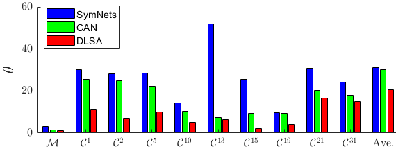
(a) Estimated angle $\theta$

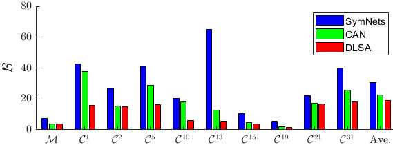
(b) Estimated intercept differences $\mathcal{B}$

Figure 3: Least squares parameters comparison of task A$\shortrightarrow$D in the Office-31 dataset. (a) is the estimated angle $\theta$ of fitting lines between source and target domains. (b) is estimated intercept differences. DLSA consistently shows the smallest estimated parameters than CAN [Kang et al.(2019)Kang, Jiang, Yang, and Hauptmann], and SymNets [Zhang et al.(2019a)Zhang, Tang, Jia, and Tan]. Ave. is the mean of 31 classes of $\theta_{\mathcal{C}}^{c}$ or $\mathcal{B}_{\mathcal{C}}^{c}$.

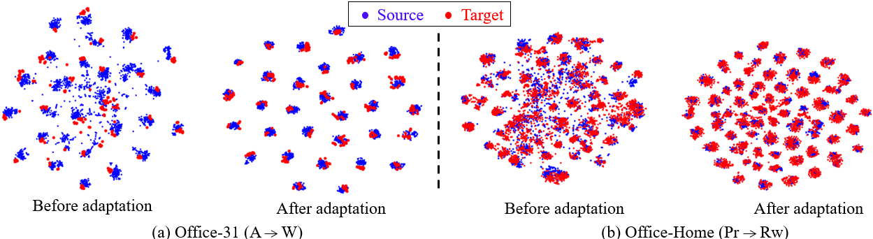
Figure 4: Visualization of learned features using a 2D t-SNE view of Office-31 and Office-Home dataset.

To further investigate whether $\theta$ and $\mathcal{B}$ are minimized using DLSA, we also compare it with top baseline methods CAN [Kang et al.(2019)Kang, Jiang, Yang, and Hauptmann] and SymNets [Zhang et al.(2019a)Zhang, Tang, Jia, and Tan] with randomly selected task A$\shortrightarrow$D in Office-31 dataset in Fig. 3 (9 of 31 classes of conditional distribution are randomly reported). We can find that the estimated parameters $\theta$ and $\mathcal{B}$ are consistently smaller than the other two methods. Hence, we can find that DLSA can minimize marginal and conditional distribution discrepancy between two domains.

Feature Visualization.

To intuitively present adaptation performance, we utilize t-SNE to visualize the deep features of network activations in 2D space before and after distribution adaptation. Fig. 4 shows two tasks: (a) A$\shortrightarrow$W of Office-31 and (b) Pr$\shortrightarrow$Rw of Office-Home dataset. Apparently, the distributions of the two tasks become more discriminative after adaptation, while many categories are mixed up in the feature space before adaptation. It indicates that DLSA can learn more discriminative representations, which can significantly increase inter-class dispersion and intra-class compactness.

5 Discussion

In these experiments, DLSA always achieves the highest average accuracy. Therefore, the quality of our model exceeds that of SOTA methods, which reveals that DLSA can better learn domain invariant features and exceeds the frequently used MMD loss and CORAL loss. There are two reasons for this. First, DLSA can estimate the latent space distribution, which is parameterized by slope and intercept. Secondly, to reduce the discrepancy between domains in the latent feature space, we align the marginal distributions by reducing the angle and intercept differences between fitting lines of the domains. In addition, conditional distribution alignment is realized by generating soft pseudo labels. Then the categorical angle and intercept differences are minimized, which further supports agreement in label space. In terms of time, the major cost of estimating slope and intercept is in Eq. LABEL:eq:parae, which can be calculated in $\mathbb{O}(1)$. More comparisons can be found in supplementary material.

However, one disadvantage of our DLSA model is that we assume a linear relationship in the latent space. Other relationships may also improve the performance (e.g., polynomial/nonlinear). Also, incorrect pseudo-labels may exist during training, affecting the quality of the fitting line as shown in Tab. 6. We can find that there are small differences of estimated parameters ($\theta_{\mathcal{C}}$ and $B_{\mathcal{C}}$) using pseudo-labels versus true labels from the target domain. Therefore, we can still improve the prediction using better pseudo-label generation methods. Removing outlier labels in the target domain might improve performance. We leave this to future work.

Table 6: Least squares estimated conditional parameters of task C$\shortrightarrow$W on Office + Caltech-10 dataset using pseudo and true target labels ($\mathcal{C}^{c}$: conditional distribution of each class $c$, where $c=\{1,2,3,\cdots,10\}$).

Parameters	$\mathcal{C}^{1}$	$\mathcal{C}^{2}$	$\mathcal{C}^{3}$	$\mathcal{C}^{4}$	$\mathcal{C}^{5}$	$\mathcal{C}^{6}$	$\mathcal{C}^{7}$	$\mathcal{C}^{8}$	$\mathcal{C}^{9}$	$\mathcal{C}^{10}$	Ave.
$\theta_{\mathcal{C}}^{\text{pseudo}}$	29.786	35.871	24.615	16.451	7.202	11.924	37.778	0.355	33.137	16.594	21.371
$\theta_{\mathcal{C}}^{\text{true}}$	31.847	36.301	26.824	17.730	7.074	9.634	36.169	0.726	35.393	18.824	22.052
$\mathcal{B}_{\mathcal{C}}^{\text{pseudo}}$	33.137	9.875	17.656	3.622	3.626	0.250	15.820	3.097	3.358	16.237	10.668
$\mathcal{B}_{\mathcal{C}}^{\text{true}}$	30.936	10.159	19.546	5.778	2.557	0.337	13.239	5.036	4.088	19.536	11.121

6 Conclusion

In this paper, we propose a novel unsupervised domain adaptation method, namely deep least squares adaptation. DLSA estimates the latent space distribution by finding the fitting lines of two domains. We then develop marginal and conditional adaptation loss to reduce domain discrepancy and learn domain invariant features. Experiential results illustrate the superiority of DLSA in modeling the source and target domain distributions, resulting in outstanding performances on benchmark datasets.

References

- [Chen et al.(2019)Chen, Xie, Huang, Rong, Ding, Huang, Xu, and Huang] C. Chen, W. Xie, W. Huang, Y. Rong, X. Ding, Y. Huang, T. Xu, and J. Huang. Progressive feature alignment for unsupervised domain adaptation. In Proc. IEEE Conf. on Computer Vision and Pattern Recognition, pages 627–636, 2019.
- [Ganin et al.(2016)Ganin, Ustinova, Ajakan, Germain, Larochelle, Laviolette, Marchand, and Lempitsky] Y. Ganin, E. Ustinova, H. Ajakan, P. Germain, H. Larochelle, F. Laviolette, M. Marchand, and V. Lempitsky. Domain-adversarial training of neural networks. The Journal of Machine Learning Research, 17(1):2096–2030, 2016.
- [Ghifary et al.(2014)Ghifary, Kleijn, and Zhang] M. Ghifary, W. B. Kleijn, and M. Zhang. Domain adaptive neural networks for object recognition. In Proceedings of the Pacific Rim International Conference on Artificial Intelligence, pages 898–904. Springer, 2014.
- [Gong et al.(2012)Gong, Shi, Sha, and Grauman] B. Gong, Y. Shi, F. Sha, and K. Grauman. Geodesic flow kernel for unsupervised domain adaptation. In Proceedings of IEEE Conference on Computer Vision and Pattern Recognition (CVPR), pages 2066–2073. IEEE, 2012.
- [Goodfellow et al.(2014)Goodfellow, Pouget-Abadie, Mirza, Xu, Warde-Farley, Ozair, Courville, and Bengio] I. Goodfellow, J. Pouget-Abadie, M. Mirza, B. Xu, D. Warde-Farley, S. Ozair, A. Courville, and Y. Bengio. Generative adversarial nets. In Advances in Neural Information Processing Systems, pages 2672–2680, 2014.
- [Gu et al.(2020)Gu, Sun, and Xu] X. Gu, J. Sun, and Z. Xu. Spherical space domain adaptation with robust pseudo-label loss. In Proceedings of the IEEE/CVF Conference on Computer Vision and Pattern Recognition, pages 9101–9110, 2020.
- [He et al.(2016)He, Zhang, Ren, and Sun] K. He, X. Zhang, S. Ren, and J. Sun. Deep residual learning for image recognition. In Proceedings of the IEEE Conference on Computer Vision and Pattern Recognition (CVPR), pages 770–778, 2016.
- [Huang et al.(2020)Huang, Chen, Li, Chen, Yuan, and Shi] G. Huang, X. Chen, L. Li, X. Chen, L. Yuan, and W. Shi. Domain adaptive partial least squares regression. Chemometrics and Intelligent Laboratory Systems, 201:103986, 2020.
- [Kang et al.(2019)Kang, Jiang, Yang, and Hauptmann] G. Kang, L. Jiang, Y. Yang, and A. G. Hauptmann. Contrastive adaptation network for unsupervised domain adaptation. In Proc. of the IEEE Conference on Computer Vision and Pattern Recognition, pages 4893–4902, 2019.
- [Krizhevsky et al.(2012)Krizhevsky, Sutskever, and Hinton] A. Krizhevsky, I. Sutskever, and G. E. Hinton. ImageNet classification with deep convolutional neural networks. In Advances in Neural Information Processing Systems, pages 1097–1105, 2012.
- [Li et al.(2020a)Li, Zhai, Luo, Ge, and Ren] M. Li, Y. Zhai, Y. Luo, P. Ge, and C. Ren. Enhanced transport distance for unsupervised domain adaptation. In Proceedings of the IEEE/CVF Conference on Computer Vision and Pattern Recognition, pages 13936–13944, 2020a.
- [Li et al.(2020b)Li, Liu, Lin, Xie, Ding, Huang, and Tang] S. Li, C. H. Liu, Q. Lin, B. Xie, Z. Ding, G. Huang, and J. Tang. Domain conditioned adaptation network. In AAAI, pages 11386–11393, 2020b.
- [Liang et al.(2020)Liang, Hu, and Feng] J. Liang, D. Hu, and J. Feng. Do we really need to access the source data? source hypothesis transfer for unsupervised domain adaptation. In International Conference on Machine Learning, pages 6028–6039. PMLR, 2020.
- [Liu et al.(2019)Liu, Long, Wang, and Jordan] H. Liu, M. Long, J. Wang, and M. Jordan. Transferable adversarial training: A general approach to adapting deep classifiers. In International Conference on Machine Learning, pages 4013–4022, 2019.
- [Long et al.(2015)Long, Cao, Wang, and Jordan] M. Long, Y. Cao, J. Wang, and M. I. Jordan. Learning transferable features with deep adaptation networks. In International conference on machine learning, pages 97–105. PMLR, 2015.
- [Long et al.(2016)Long, Zhu, Wang, and Jordan] M. Long, H. Zhu, J. Wang, and M. I. Jordan. Unsupervised domain adaptation with residual transfer networks. In Advances in Neural Information Processing Systems, pages 136–144, 2016.
- [Long et al.(2017)Long, Zhu, Wang, and Jordan] M. Long, H. Zhu, J. Wang, and M. I. Jordan. Deep transfer learning with joint adaptation networks. In Proceedings of the 34th International Conference on Machine Learning, volume 70, pages 2208–2217. JMLR.org, 2017.
- [Long et al.(2018)Long, Cao, Wang, and Jordan] M. Long, Z. Cao, J. Wang, and M. I. Jordan. Conditional adversarial domain adaptation. In Advances in Neural Information Processing Systems, pages 1647–1657, 2018.
- [Lu et al.(2020)Lu, Yang, Zhu, Liu, Song, and Xiang] Z. Lu, Y. Yang, X. Zhu, C. Liu, Y.-Z. Song, and T. Xiang. Stochastic classifiers for unsupervised domain adaptation. In Proceedings of the IEEE/CVF Conference on Computer Vision and Pattern Recognition, pages 9111–9120, 2020.
- [Luo et al.(2020)Luo, Ren, DAI, and Yan] Y. Luo, C. Ren, D. DAI, and H. Yan. Unsupervised domain adaptation via discriminative manifold propagation. IEEE Transactions on Pattern Analysis and Machine Intelligence, 2020.
- [Mao et al.(2017)Mao, Li, Xie, Lau, Wang, and Paul Smolley] X. Mao, Q. Li, H. Xie, R. Y. Lau, Z. Wang, and S. Paul Smolley. Least squares generative adversarial networks. In Proceedings of the IEEE international conference on computer vision, pages 2794–2802, 2017.
- [Meng et al.(2018)Meng, Li, Gong, and Juang] Z. Meng, J. Li, Y. Gong, and B. Juang. Adversarial teacher-student learning for unsupervised domain adaptation. In 2018 IEEE International Conference on Acoustics, Speech and Signal Processing (ICASSP), pages 5949–5953. IEEE, 2018.
- [Nikzad-Langerodi et al.(2020)Nikzad-Langerodi, Zellinger, Saminger-Platz, and Moser] R. Nikzad-Langerodi, W. Zellinger, S. Saminger-Platz, and B. A. Moser. Domain adaptation for regression under beer–lambert’s law. Knowledge-Based Systems, 210:106447, 2020.
- [Peng et al.(2017)Peng, Usman, Kaushik, Hoffman, Wang, and Saenko] X. Peng, B. Usman, N. Kaushik, J. Hoffman, D. Wang, and K. Saenko. Visda: The visual domain adaptation challenge. arXiv preprint arXiv:1710.06924, 2017.
- [Rahman et al.(2020)Rahman, Fookes, Baktashmotlagh, and Sridharan] M. M. Rahman, C. Fookes, M. Baktashmotlagh, and S. Sridharan. On minimum discrepancy estimation for deep domain adaptation. In Domain Adaptation for Visual Understanding, pages 81–94. Springer, 2020.
- [Saenko et al.(2010)Saenko, Kulis, Fritz, and Darrell] K. Saenko, B. Kulis, M. Fritz, and T. Darrell. Adapting visual category models to new domains. In Proceedings of the European Conference on Computer Vision, pages 213–226. Springer, 2010.
- [Saito et al.(2018)Saito, Watanabe, Ushiku, and Harada] K. Saito, K. Watanabe, Y. Ushiku, and T. Harada. Maximum classifier discrepancy for unsupervised domain adaptation. In Proceedings of the IEEE Conference on Computer Vision and Pattern Recognition, pages 3723–3732, 2018.
- [Sun and Saenko(2016)] B. Sun and K. Saenko. Deep coral: Correlation alignment for deep domain adaptation. In Proc. of European Conference on Computer Vision, pages 443–450. Springer, 2016.
- [Tang and Jia(2020)] H. Tang and K. Jia. Discriminative adversarial domain adaptation. In Proceedings of the AAAI Conference on Artificial Intelligence, volume 34, pages 5940–5947, 2020.
- [Tzeng et al.(2014)Tzeng, Hoffman, Zhang, Saenko, and Darrell] E. Tzeng, J. Hoffman, N. Zhang, K. Saenko, and T. Darrell. Deep domain confusion: Maximizing for domain invariance. arXiv preprint arXiv:1412.3474, 2014.
- [Tzeng et al.(2017)Tzeng, Hoffman, Saenko, and Darrell] E. Tzeng, J. Hoffman, K. Saenko, and T. Darrell. Adversarial discriminative domain adaptation. In Proceedings of the IEEE Conference on Computer Vision and Pattern Recognition, pages 7167–7176, 2017.
- [Venkateswara et al.(2017)Venkateswara, Eusebio, Chakraborty, and Panchanathan] H. Venkateswara, J. Eusebio, S. Chakraborty, and S. Panchanathan. Deep hashing network for unsupervised domain adaptation. In Proceedings of the IEEE Conference on Computer Vision and Pattern Recognition, pages 5018–5027, 2017.
- [Wang et al.(2018)Wang, Feng, Chen, Yu, Huang, and Yu] J. Wang, W. Feng, Y. Chen, H. Yu, M. Huang, and P. S. Yu. Visual domain adaptation with manifold embedded distribution alignment. In Proceedings of the 26th ACM International Conference on Multimedia, MM ’18, pages 402–410, 2018. 10.1145/3240508.3240512.
- [Wang(2020)] T. Wang, Q.and Breckon. Unsupervised domain adaptation via structured prediction based selective pseudo-labeling. In Proceedings of the AAAI Conference on Artificial Intelligence, volume 34, pages 6243–6250, 2020.
- [Wang et al.(2019)Wang, Li, Ye, Long, and Wang] X. Wang, L. Li, W. Ye, M. Long, and J. Wang. Transferable attention for domain adaptation. In Proceedings of the AAAI Conference on Artificial Intelligence, volume 33, pages 5345–5352, 2019.
- [Wu et al.(2020)Wu, Inkpen, and El-Roby] Y. Wu, D. Inkpen, and A. El-Roby. Dual mixup regularized learning for adversarial domain adaptation. In European Conference on Computer Vision, pages 540–555. Springer, 2020.
- [Xu et al.(2019)Xu, Zhang, Ni, Li, Wang, Tian, and Zhang] M. Xu, J. Zhang, B. Ni, T. Li, C. Wang, Q. Tian, and W. Zhang. Adversarial domain adaptation with domain mixup. arXiv preprint arXiv:1912.01805, 2019.
- [Yuan et al.(2020)Yuan, Li, Zhu, Li, and Gu] Y. Yuan, Y. Li, Z. Zhu, R. Li, and X. Gu. Adversarial joint domain adaptation of asymmetric feature mapping based on least squares distance. Pattern Recognition Letters, 136:251–256, 2020.
- [Zhang et al.(2017)Zhang, Li, and Ogunbona] J. Zhang, W. Li, and P. Ogunbona. Joint geometrical and statistical alignment for visual domain adaptation. In Proceedings of the IEEE Conference on Computer Vision and Pattern Recognition, pages 1859–1867, 2017.
- [Zhang and Davison(2019)] Y. Zhang and B. D. Davison. Modified distribution alignment for domain adaptation with pre-trained Inception ResNet. arXiv preprint arXiv:1904.02322, 2019.
- [Zhang and Davison(2020a)] Y. Zhang and B. D. Davison. Adversarial consistent learning on partial domain adaptation of plantclef 2020 challenge. In CLEF working notes 2020, CLEF: Conference and Labs of the Evaluation Forum, 2020a.
- [Zhang and Davison(2020b)] Y. Zhang and B. D. Davison. Adversarial continuous learning on unsupervised domain adaptation. In 25th International Conference on Pattern Recognition Workshops, pages 672–687, 2020b.
- [Zhang and Davison(2020c)] Y. Zhang and B. D. Davison. Domain adaptation for object recognition using subspace sampling demons. Multimedia Tools and Applications, pages 1–20, 2020c.
- [Zhang and Davison(2020d)] Y. Zhang and B. D. Davison. Impact of ImageNet model selection on domain adaptation. In Proceedings of the IEEE Winter Conference on Applications of Computer Vision Workshops, pages 173–182, 2020d.
- [Zhang and Davison(2021a)] Y. Zhang and B. D. Davison. Deep spherical manifold gaussian kernel for unsupervised domain adaptation. In Proceedings of the IEEE/CVF Conference on Computer Vision and Pattern Recognition Workshops (CVPRW), pages 4443–4452, 2021a.
- [Zhang and Davison(2021b)] Y. Zhang and B. D. Davison. Efficient pre-trained features and recurrent pseudo-labeling in unsupervised domain adaptation. In Proceedings of the IEEE/CVF Conference on Computer Vision and Pattern Recognition Workshops (CVPRW), pages 2719–2728, 2021b.
- [Zhang and Davison(2021c)] Y. Zhang and B. D. Davison. Enhanced separable disentanglement for unsupervised domain adaptation. In 2021 IEEE International Conference on Image Processing (ICIP), pages 784–788, 2021c.
- [Zhang et al.(2019a)Zhang, Tang, Jia, and Tan] Y. Zhang, H. Tang, K. Jia, and M. Tan. Domain-symmetric networks for adversarial domain adaptation. In Proceedings of the IEEE Conference on Computer Vision and Pattern Recognition, pages 5031–5040, 2019a.
- [Zhang et al.(2019b)Zhang, Xie, and Davison] Y. Zhang, S. Xie, and B. D. Davison. Transductive learning via improved geodesic sampling. In Proceedings of the 30th British Machine Vision Conference, 2019b.
- [Zhang et al.(2021)Zhang, Ye, and Davison] Y. Zhang, H. Ye, and B. D. Davison. Adversarial reinforcement learning for unsupervised domain adaptation. In Proceedings of the IEEE/CVF Winter Conference on Applications of Computer Vision, pages 635–644, 2021.