Shell-model study of titanium isotopic chain with chiral two- and three-body forces

Abstract

The even-even Ti isotopic chain, from $A=42$ to 70, has been studied within the nuclear shell-model framework by employing an effective Hamiltonian which is derived by way of many-body perturbation theory from a chiral potential with two- and three-body forces, and includes three-body contributions which account for Pauli principle violations in nuclei with more than two valence particles. We consider ⁴⁰Ca as a closed core and a model space spanned by the neutron and proton $0f1p$ orbitals with the addition of the $0g_{9/2}$ orbital for neutrons. Calculated two-neutron separation energies and excitation energies of the yrast $2^{+}$ states are reported and compared with the experimental data, which are available up to ⁶²Ti. The present study intends to investigate the effects of the adopted effective interactions on the evolution of the shell structure.

I Introduction

In the last two decades or so, a large amount of data provided by radioactive ion beam facilities has refined our vision of the nuclear shell structure. The existence of the magic numbers associated with 2, 8, 20, 28, 50, 82 protons or neutrons, and 126 neutrons has been the cornerstone of the shell model for many years starting from its entry into nuclear physics by Mayer and Jensen Mayer (1949); Haxel et al. (1949). The new data have put into evidence that magic numbers are not universal, but they may change as a function of $N$ and $Z$ when going far from the stability line. For instance, new shell gaps have been identified at $N=32,34$ in neutron-rich nuclei with $Z\approx 20$ and at $N=16$ for O isotopes, while the disappearance or weakening of canonical magic numbers has been observed in lighter nuclei at $N=8$, $N=20$, and $N=28$ (see, for instance, Refs.Huck et al. (1985); Motobayashi et al. (1995); Navin et al. (2000); Iwasaki et al. (2000); Janssens et al. (2002); Shimoura et al. (2003); Dinca et al. (2005); Bürger et al. (2005); Gade et al. (2006); Bastin et al. (2007); Hoffman et al. (2009); Kanungo et al. (2009); Takeuchi et al. (2012); Wienholtz et al. (2013); Steppenbeck et al. (2013); Liu et al. (2019)). Nowadays, great theoretical and experimental efforts are devoted to study the evolution of the shell structure and, in particular, to identify the behavior of shell gaps along isotopic chains as well as to understand the role played by the different components of the nuclear force in driving their modifications.

In particular, the Ca isotopic chain, with magic proton number $Z=20$, has attracted considerable interest, since it exhibits two neutron shell closures at $N=32$ Huck et al. (1985); Gade et al. (2006); Wienholtz et al. (2013) and 34 Steppenbeck et al. (2013) in addition to the standard one at $N=28$. Special attention is presently focused on the very exotic ⁶⁰Ca with the aim to acquire information useful to investigate the shell structure evolution at $N=40$ and shed light on the possible doubly magic nature of this nucleus. From the experimental point of view the existence of ⁶⁰Ca has been only recently established Tarasov et al. (2018), but no information is available on the excitation energy of the yrast $2^{+}$ state. It is worth mentioning also that the experimental location of the neutron drip line in Ca isotopes is still unknown, and no clear indications emerge from theory Meng et al. (2002); Holt et al. (2012); Hagen et al. (2012); Hergert et al. (2014); Neufcourt et al. (2019); Cao et al. (2019); Li et al. (2020).

On the other hand, the shell closure at $N=40$ observed in ⁶⁸Ni, which corresponds to the filling of the neutron $0f1p$ and proton $0f_{7/2}$ orbitals, rapidly disappears when removing protons from $0f_{7/2}$, as it is shown by the behavior of the experimental excitation energies of the yrast $J^{\pi}=2^{+}$ states in iron and chromium neutron-rich isotopes.

In this context, also the chain of Ti isotopes ($Z=22$) represents a key piece to investigate the evolution of the shell structure towards $Z=20$. The properties of these nuclei, especially those for $N\approx 40$, may provide a more sound testing ground of nuclear models and of their predictions of the Ca drip line.

Experimental data are now known for Ti isotopes from $A=42$ to 62. The masses of ^60,62Ti were determined for the first time through the measurements reported in Ref. Michimasa et al. (2020), while the $2^{+}_{1}\rightarrow 0^{+}_{gs}$ and $4^{+}_{1}\rightarrow 2^{+}_{1}$ transitions in ⁶⁰Ti and ⁶²Ti were observed via one-proton stripping reactions from ⁶¹V and ⁶³V, respectively, in Refs. Gade et al. (2014); Cortès et al. (2020). These experiments show an increase in the $2^{+}_{1}$ excitation energies of both nuclei as compared with the corresponding Cr and Fe isotones, which indicates a decrease in collectivity towards $Z=20$. However, the reduced size in the increase does not seem to support the existence of a shell closure at $N=40$ for ⁶⁰Ca.

From the theoretical point of view, several shell-model (SM) calculations have been carried out for Ti nuclei by considering various model spaces referred to both ⁴⁰Ca or ⁴⁸Ca as closed core and employing empirically corrected interactions Poves et al. (2005); Honma et al. (2005); Dinca et al. (2005); Lenzi et al. (2010); Suzuki et al. (2013); Wimmer et al. (2019); Gade et al. (2014); Cortès et al. (2020). In Ref. Coraggio et al. (2014), some of the present authors performed a study of isotopic chains ”north-east” of ⁴⁸Ca, including Ti isotopes, by employing two-body matrix elements of the residual interaction derived from the high-precision CD-Bonn free nucleon-nucleon potential.

In the present paper, the whole even-even titanium isotopic chain from $A=42$ to 70 has been studied for the first time within the realistic SM framework starting from up-to-date two- and three-body forces derived in the framework of chiral perturbation theory (ChPT). The SM effective Hamiltonian, consisting of the single-particle (SP) energies and the two-body matrix elements (TBMEs), is built up using the many-body perturbation theory Kuo et al. (1971); Coraggio and Itaco (2020), and includes the effect of second-order three-body diagrams arising in nuclei with more than two valence particles, which account for three-body correlations induced by the interaction via the two-body force of clusters of three-valence nucleons with core excitations as well as with virtual intermediate nucleons scattered above the model space.

This work follows two of our previous studies. In the first one  Ma et al. (2019), we investigated the role played by genuine and effective chiral three-body forces in providing a reliable monopole component of the SM effective Hamiltonian defined in the $0f1p$ model space. Results are discussed for $Z=20$, 22, 24, 26, 28 with $N$ from 22 to 40. In the second one  Coraggio et al. (2020), focused only on Ca isotopes, the same approach was used in a larger model space including the neutron $0g_{9/2}$ orbital to describe isotopes beyond $N=40$. Here, we move a step forward to test our approach along an extensive isotopic chain, as Ti nuclei, with both valence neutrons and protons.

It is worth mentioning that two- and three-body chiral forces have been also used in some recent ab initio calculations for Ti isotopes. In Ref. Hagen et al. (2012), the authors investigated ^50,54,56Ti by way of the coupled-cluster method including the coupling to the particle continuum, while in Ref. Xu et al. (2019) the shell gap in ⁵⁴Ti was analyzed in terms of valence-space in-medium similarity renormalization group (VS-IMSRG). The latter was also used in Ref. Stroberg et al. (2021) to investigate the properties of nuclei from helium to iron. Precision mass measurements of ^51-55Ti were performed in Ref. Leistenschneider et al. (2018) and compared with the predictions of multireference in-medium similarity renormalization group (MR-IMSRG), VS-IMSRG, and self-consistent Gorkov-Green’s function (GGF) calculations. Furthermore, VS-IMSRG results are reported in Ref. Cortès et al. (2020) for the excitation energies of the new observed $2^{+}$ and $4^{+}$ states in ⁶²Ti, together with predictions of beyond mean-field and large-scale SM calculations, the latter being based on the same model space and effective interaction of Ref. Lenzi et al. (2010). The comparison with experiment shows that only large-scale SM calculations reproduce very accurately data for ⁶²Ti, which are instead largely overestimated by the other two approaches. The theoretical framework of Ref. Lenzi et al. (2010) gives also a good description of the experimental excitation energies of ⁶⁰Ti, as shown in Ref. Gade et al. (2014).

In concluding this section, it has to be pointed out that, similarly to our previous study on Ca isotopes Coraggio et al. (2020), we do not include in the model space the neutron $1d_{5/2}$ orbital, which was shown to be of great importance to reproduce the onset of the collectivity at $N=40$ for isotopic chains ”north-east” of ⁴⁸Ca, as first discussed in Ref. Caurier et al. (2002) and then confirmed in Refs. Lenzi et al. (2010); Coraggio et al. (2014); Wimmer et al. (2019); Gade et al. (2014); Cortès et al. (2020).

In Ref. Zuker et al. (1995), the authors have identified the source of this collective behavior as a consequence of the quasi-SU(3) approximate symmetry, owing to the interplay between the quadrupole-quadrupole component of the residual interaction and the central field in the sub-space spanned by the lowest $\Delta j$=2 orbitals of a major shell.

In particular, in Ref. Lenzi et al. (2010) -where the adopted model space was based on a ⁴⁸Ca core including the $1p0f$ shell for protons and the $1p,0f_{5/2},0g_{9/2},1d_{5/2}$ orbitals for neutrons - the deformation driving role of the neutron $1d_{5/2}$ orbital below ⁶⁸Ni was assessed showing that the maximum deformation develops in ⁶⁴Cr and decreases towards Ca. Such a situation was, in fact, explained in terms of a reduction of the neutron $0f_{5/2}-0g_{9/2}$ gap when protons are removed from the $0f_{7/2}$ orbital, which is accompanied by an enhancement of the quadrupole-quadrupole correlations between the neutron $0g_{9/2}$ and $1d_{5/2}$ orbitals. Similar results are shown in Ref. Coraggio et al. (2014) where the Ca, Ti, Fe Cr, Ni isotopic chains ”north-east” of ⁴⁸Ca were studied within the realistic SM framework, by comparing the results for two model spaces differing for the inclusion of the neutron $1d_{5/2}$ orbital.

A model space space starting from ⁴⁰Ca as closed core and including the neutron $1d_{5/2}$ makes calculations around $N=40$ very cumbersome. Dimensions of the Hamiltonian matrix reach about $10^{11}$ in the case of ⁶²Ti, which represents the limit of our computing power. Our choice to exclude the neutron $1d_{5/2}$ orbital is, therefore, related essentially to this reason. We plan to overcome this limit by extending the so-called double-step procedure introduced in Refs. Coraggio et al. (2015, 2016) to reduce the computational complexity of large-scale SM calculations, which consists in deriving an effective Hamiltonian within a manageable model space by means of a unitary transformation of a large-scale Hamiltonian.

Nevertheless, the present study, in parallel with our previous one on Ca isotopes, intends to investigate the effects of our SM effective interactions on the evolution of the shell structure before tackling the problem in a larger model space including the neutron $1d_{5/2}$ orbital.

In the following section, we give an outline of the theoretical framework in which our SM calculations are performed. Results for the excitation energies of the yrast $2^{+}$ states and two-neutron separation energies of even-even Ti nuclei from $N=20$ to 48 are presented and compared with the available experimental data in Sec. III. In this section, we also discuss the sensitivity of these results with respect to the many-body correlations and their impact on the effective-single particle energies. Section IV provides a summary and concluding remarks.

II Outline of the theoretical framework

As mentioned in the Introduction, SM calculations for Ti isotopes have been performed within the same approach as Ref. Coraggio et al. (2020), which we refer for more details. Calculations are performed by means of the SM code KSHELL Shimizu et al. (2019) in the model space spanned by the four proton $0f_{7/2}$, $0f_{5/2}$, $1p_{3/2}$, $1p_{1/2}$ orbitals and the five neutron $0f_{7/2}$, $0f_{5/2}$, $1p_{3/2}$, $1p_{1/2}$, $0g_{9/2}$ orbitals outside the doubly magic ⁴⁰Ca.

We start our calculation from the nucleon-nucleon ($NN$) potential developed by Entem and Machleidt Entem and Machleidt (2002) within chiral perturbation theory at next-to-next-to-next-to-leading order (N³LO) and the chiral three-body ($NNN$) potential at next-to-next-to-leading order (N²LO), which share the same nonlocal regulator function. The low-energy constants (LECs) appearing in both $NN$ and $NNN$ components, namely $c_{1}$, $c_{3}$, $c_{4}$, are determined by the renormalization procedure described in Ref. Machleidt and Entem (2011), while for the $c_{D}$ and $c_{E}$ LECs characterizing only the $NNN$ force we take the values of Ref. Navrátil et al. (2007).

The matrix elements of the $NN$ and $NNN$ forces, with the addition of the Coulomb one in the proton-proton channel, are computed in the harmonic oscillator basis with an oscillator parameter $\hbar\omega=45A^{-1/3}-25A^{-2/3}$ for $A=40$. Details of the calculation of matrix elements of the N²LO $NNN$ potential are reported in Ref. Fukui et al. (2018).

These matrix elements are used as input to derive the SM effective Hamiltonian $H_{\rm eff}$  within the time-dependent perturbation theory. Specifically, $H_{\rm eff}$  is expressed by way of the Kuo-Lee-Ratcliff folded-diagram expansion Kuo et al. (1971) in terms of the $\hat{Q}$-box vertex function, which is defined as

$$\hat{Q}(\epsilon)=PH_{1}P+PH_{1}Q\frac{1}{\epsilon-QHQ}QH_{1}P~{},$$ (1)

where $H$ is the full nuclear Hamiltonian $H=H_{0}+H_{1}$, $H_{0}$ and $H_{1}$ being the unperturbed and the interaction components, respectively, and $\epsilon$ an energy parameter called starting energy”.

Then, the $\hat{Q}$-box may be calculated by expanding the term $1/(\epsilon-QHQ)$ as a power series

$$\frac{1}{\epsilon-QHQ}=\sum_{n=0}^{\infty}\frac{1}{\epsilon-QH_{0}Q}\left(\frac{QH_{1}Q}{\epsilon-QH_{0}Q}\right)^{n}~{}.$$ (2)

This provides a perturbative expansion of the $\hat{Q}$-box, and its diagrammatic representation is given as a collection of irreducible valence-linked Goldstone diagrams Kuo et al. (1971).

Once the $\hat{Q}$-box is calculated, $H_{\rm eff}$ is obtained solving nonlinear matrix equations by way of iterative techniques such as the Kuo-Krenciglowa and Lee-Suzuki ones Suzuki and Lee (1980), or graphical noniterative methods Suzuki et al. (2011). The latter is the method we have employed in present work, since it results in a faster and more stable convergence to the solution of the matrix equations.

We arrest the $\hat{Q}$-box expansion of the one- and two-body Goldstone diagrams at third order in the $NN$ potential and at first order in the $NNN$ one. It has to be pointed out that the diagrams at first order in $NNN$ potential - whose analytical expressions are reported in Refs. Fukui et al. (2018); Ma et al. (2019) - are the coefficients of the one-body and two-body terms arising from the normal-ordering decomposition of the three-body component of a many-body Hamiltonian Hjorth-Jensen et al. (2017).

Since our goal is the study of the Ti isotopic chain up to ⁷⁰Ti, we are going to diagonalize the SM Hamiltonian for systems up to thirty valence nucleons. This means that the derivation of the SM effective Hamiltonian needs to resolve the progressive filling of the model space orbitals, especially in the calculation of the irreducible valence-linked diagrams of the $\hat{Q}$-box.

This should be achieved by including in the $\hat{Q}$-box many-body diagrams which account for the interaction via the two-body force of the valence nucleons with configurations outside the model space, leading to a dependence of $H_{\rm eff}$ on the number of valence nucleons. We arrest the cluster expansion to the leading term, namely second-order three-body diagrams, which, for those nuclei with more than two valence nucleons, account for the interaction of the valence nucleons with core excitations as well as with virtual intermediate nucleons scattered above the model space. These diagrams are reported in Fig. 1 and their explicit expressions, $D_{A}$ and $D_{B}$, are

$$\langle\left[(j_{a}j_{b})_{J_{ab}},j_{e}\right]_{J}|D_{A}|\left[(j_{c}j_{d})_{J_{cd}},j_{f}\right]_{J}\rangle=\\ \sum_{J_{be}}\sum_{p}(-1)^{b+e+f+p}\hat{J_{ab}}\hat{J_{cd}}\hat{J_{be}}^{2}\left\{\begin{array}[]{ccc}j_{a}~{}j_{b}~{}J_{ab}\\ j_{e}~{}J~{}J_{be}\end{array}\right\}\left\{\begin{array}[]{ccc}j_{a}~{}j_{p}~{}J_{cd}\\ j_{f}~{}J~{}J_{be}\end{array}\right\}\\ ~{}\times\frac{\langle b,e;J_{be}|V_{NN}|p,f;J_{be}\rangle\langle a,p;J_{cd}|V_{NN}|c,d;J_{cd}\rangle}{[\epsilon_{0}-(\epsilon_{a}+\epsilon_{f}+\epsilon_{p})]}~{},$$ (3)

$$\langle\left[(j_{a}j_{b})_{J_{ab}},j_{e}\right]_{J}|D_{B}|\left[(j_{c}j_{d})_{J_{cd}},j_{f}\right]_{J}\rangle=\\ \sum_{J_{be}}\sum_{h}(-1)^{b+e+f+h+1}\hat{J_{ab}}\hat{J_{cd}}\hat{J_{be}}^{2}\left\{\begin{array}[]{ccc}j_{a}~{}j_{b}~{}J_{ab}\\ j_{e}~{}J~{}J_{be}\end{array}\right\}\left\{\begin{array}[]{ccc}j_{a}~{}j_{h}~{}J_{cd}\\ j_{f}~{}J~{}J_{be}\end{array}\right\}\\ ~{}\times\frac{\langle b,e;J_{be}|V_{NN}|h,f;J_{be}\rangle\langle a,h;J_{cd}|V_{NN}|c,d;J_{cd}\rangle}{[\epsilon_{0}-(\epsilon_{a}+\epsilon_{b}+\epsilon_{d}+\epsilon_{f}-\epsilon_{h})]}~{},$$ (4)

where the indices $a,b,c,d,e,f,p,h$ refer to the quantum numbers of the incoming, outcoming, and intermediate single-particle states, $\epsilon_{m}$ denotes the unperturbed single-particle energy of the orbital $j_{m}$, $\epsilon_{0}$ is the so-called starting energy, namely the unperturbed energy of the incoming particles $\epsilon_{0}=\epsilon_{c}+\epsilon_{d}+\epsilon_{f}$.

From now on, we dub these contributions 3-b correlations .

Figure 1: Second-order three-body diagrams. The sum over the intermediate lines runs over particle and hole states outside the model space, shown by $A$ and $B$, respectively. We report only one of the nine existing topologies which correspond to the permutations of the external lines.

We also point out that for each topology reported in Fig. 1, there are nine diagrams, corresponding to the possible permutations of the external lines Polls et al. (1983).

Diagrams $A,B$ include the effects of the Pauli blocking due to the filling of the valence particle lines in the second-order ladder and core-polarization diagrams Ellis and Osnes (1977), respectively, quenching the contribution of these two-body terms.

Nevertheless, the KSHELL SM code, which we employ for the calculations, cannot perform the diagonalization of a three-body $H_{\rm eff}$, so we derive density-dependent two-body terms ($\alpha$) from the corresponding second-order three-body diagrams ($A,B$), as shown in Fig. 2.

Figure 2: Density-dependent two-body contribution that is derived from a three-body one. $\alpha$ is obtained by summing over one incoming and outgoing particle of the three-body graphs $A,B$ reported in Fig. 1.

We then calculate, for each $A,B$ topology, nine one-loop diagrams, namely the graph $(\alpha)$ in Fig. 2. Their explicit form, in terms of the three-body graphs $A,B$, is

$$\langle(j_{a}j_{b})_{J}|V^{\alpha}|(j_{c}j_{d})_{J}\rangle=\\ \sum_{m,J^{\prime}}~{}\rho_{m}\frac{\hat{J^{\prime}}^{2}}{\hat{J}^{2}}\langle\left[(j_{a}j_{b})_{J},j_{m}\right]_{J^{\prime}}|V^{A,B}|\left[(j_{c}j_{d})_{J},j_{m}\right]_{J^{\prime}}\rangle~{}~{},$$ (5)

where the summation over $m$-index runs in the model space, and $\rho_{m}$ is the unperturbed occupation density of the orbital $m$ according to the number of valence nucleons.

Following the above procedure, the perturbative expansion of the $\hat{Q}$-box contains one- and two-body diagrams up to third order in $V_{NN}$, and a density-dependent two-body contribution which accounts for three-body second-order diagrams $A,B$.

It should be stressed that the latter term depends on the number of valence protons and neutrons, thus we derive specific effective SM Hamiltonians for any nuclear system under consideration, Hamiltonians that differ only for the two-body matrix elements.

It is worth mentioning that, as done in Ref. Coraggio et al. (2020) for Ca, we have checked the effect of the spurious center-of-mass motion. In line with the previous outcome, we have found that results are only marginally affected by spurious components.

In the Supplemental Material SM we report the TBMEs of the interaction calculated without including three-body correlations as well as those of the density dependent interaction for $A=62$. Neutron and proton SP energies are shown in Table 1. It is worth mentioning that the proton and neutron SP spacings obtained from the theory are shifted to reproduce the experimental ground-state energies of ⁴¹Sc and ⁴¹Ca with respect to ⁴⁰Ca. This is because, as discussed in Ref. Coraggio et al. (2020), our derivation of the effective Hamiltonian with $N_{\rm max}=18$ does not provide convergent spectra for the one-valence systems.

Table 1: Proton $\epsilon_{b}^{\pi}$ and neutron $\epsilon^{\nu}_{b}$ single-particle energies (in MeV).

$b$	$\epsilon^{\pi}_{b}$	$\epsilon^{\nu}_{b}$
$0f_{7/2}$	$-1.1$	$-8.4$
$0f_{5/2}$	$6.2$	$-0.2$
$1p_{3/2}$	$1.4$	$-5.2$
$1p_{1/2}$	$3.3$	$-3.1$
$0g_{9/2}$	$-$	$1.5$

III Results

We start focusing on the two-neutron separation energies, whose calculated values from ⁴⁴Ti to ⁷⁰Ti are shown in Fig. 3 together with the available experimental data.

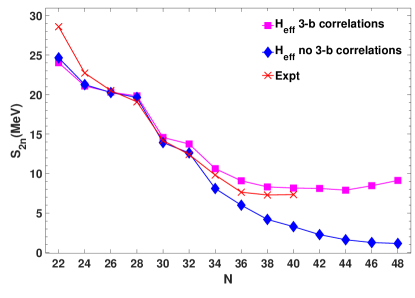
Figure 3: (Color online) Theoretical two-neutron separation energies for even-even Ti isotopes from $N=22$ to 48, with and without the 3-b correlations, are compared to the experimental data from Ref. Michimasa et al. (2020) for $N=40$ and from AME2020 Wang et al. (2021) for the other isotopes.

We see that the calculated two-neutron separation energies ($S_{2n}$), with (magenta squares) and without (blue diamonds) 3-b correlations, are in a good agreement with the experimental data (red cross) up to $N=32$. Actually, both calculations provide the observed shell closures at $N=28$ and $N=32$, which manifest as a sudden drop of $S_{2n}$ at $N=30$ and $N=34$. However, starting from $N=34$ the effect of 3-b correlations becomes rather large and, as expected, grows with increasing neutron number in analogy with the results obtained for Ca isotopes Coraggio et al. (2020). It turns out that their contribution increases the calculated $S_{2n}$, and leads to a good agreement with the measured values in ^56-62Ti, which are significantly underestimated when 3-b correlations are omitted. Nevertheless, in both calculations all Ti isotopes up to ⁷⁰Ti are predicted to be bound.

The experimental excitation energies of the yrast $2^{+}$ state are compared with the calculated values obtained with and without 3-b correlations in Fig. 4. Up to $N=38$, the results of the two calculations are very similar and do not differ significantly from those reported in Ref. Ma et al. (2019), where the model space was limited to the neutron and proton $1f1p$ orbitals. It can be seen that both calculations are in quite good agreement with experimental data up to $N=34$, and in particular predict the observed shell closures in ⁵⁰Ti and ⁵²Ti. However, from $N=36$ on, the theoretical curves start to climb towards $N=40$, at variance with the observed behavior of the yrast $2^{+}$ excitation energies that does not exhibit such a raise. This deficiency in our calculations may be ascribed to the inadequacy of the adopted model space, which does not include the neutron $1d_{5/2}$ orbital. In fact, as mentioned in the Introduction, the interaction between neutron $1d_{5/2}$ and $0g_{9/2}$ orbitals ignites a quadrupole collectivity that is responsible for the disappearance of the $N=40$ shell closure in isotopic chains ”north-east” of ⁴⁸Ca, especially in chromium and iron isotopes Caurier et al. (2002); Lenzi et al. (2010); Coraggio et al. (2014); Wimmer et al. (2019); Gade et al. (2014); Cortès et al. (2020).

Despite this unsatisfactory result, it is worth pointing out that differences emerge in the two theoretical curves starting from $N=40$ to 48. As a matter of fact, they evince that the contribution of 3-b correlations reduces the excitation energy of the $2^{+}_{1}$ state, leading to the disappearance of the shell gap in ⁶²Ti, in agreement with experiment Cortès et al. (2020).

We have found that 3-b correlations also influence the calculation of the yrast $4^{+}$ states. The predicted behavior of their excitation energies, obtained by omitting these correlations, exhibits a positive slope from ⁶⁰Ti to ⁶²Ti that is not experimentally observed. On the other hand, the experimental behavior is reproduced when 3-b correlations are included, although the calculated excitation energies underestimate the measured values by about 500 KeV along the whole chain, except for ⁴²Ti where a larger discrepancy is noticed.

The results shown above evince the effects produced on the shell structure of Ti isotopes when the evolution the SM Hamiltonian, as a function of the number of valence nucleons, is microscopically taken into account. We are confident that the combination of these correlations with the enlargement of the model space including the neutron $1d_{5/2}$ orbital is the key to reproduce the observed degree of collectivity in N$\approx$40 nuclei ”north-east” of ⁴⁸Ca.

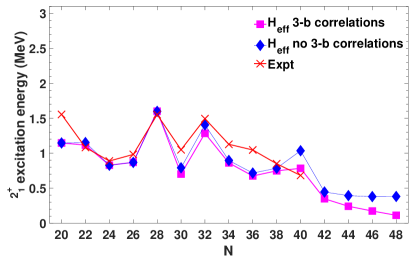
Figure 4: (Color online) Theoretical $2^{+}_{1}$ excitation energies for even-even Ti isotopes from $N=20$ to 48, with and without the 3-b correlations, are compared with the experimental data from Ref. Cortès et al. (2020) for $N=40$ and from Ref. NND for the other isotopes.

The shell evolution can be analyzed by studying the behavior of the effective single particle energies (ESPEs) along the isotopic chain, and thus we have found it interesting to see how they are influenced by 3-b correlations.

The ESPEs are defined as

$${\rm ESPE}(a^{\tau})=\epsilon_{a}^{\tau}+\sum_{b\tau^{\prime}}{\bar{V}}_{ab}^{\tau\tau^{\prime}}n_{b}^{\tau^{\prime}},$$ (6)

where $\tau$,$\tau^{\prime}$ stand for neutron or proton index and $a$,$b$ run over all the valence orbitals. The quantities $\epsilon_{a}^{\tau}$ and $n_{a}^{\tau}$ denote the SP energy and the ground-state occupation number of the $a^{\tau}$ level, while ${\bar{V}}_{ab}^{\tau\tau^{\prime}}$ is the monopole component of the two-body effective interaction $(V_{\rm eff})$ obtained by averaging on the projection of the total angular momentum and can be written as

$${\bar{V}}_{ab}^{\tau\tau^{\prime}}=\frac{\sum_{J}(2J+1)\langle a^{\tau},b^{\tau^{\prime}}\mid V_{\rm eff}\mid a^{\tau},b^{\tau^{\prime}}\rangle_{J}}{\sum_{J}(2J+1)},$$ (7)

where $J$ runs over Pauli allowed values.

The proton ESPEs are not significantly affected by 3-b correlations. In both calculations, the proton $0f^{\pi}_{7/2}$ orbital is well separated from the other ones, and the $1p^{\pi}_{3/2}-0f^{\pi}_{7/2}$ gap increases towards neutron rich Ti isotopes, which indicates the stability of the shell closure at $Z=28$. The other SP states are close each other with the inversion of $1p^{\pi}_{1/2}$ and $0f^{\pi}_{5/2}$ orbitals in correspondence of $N=40$.

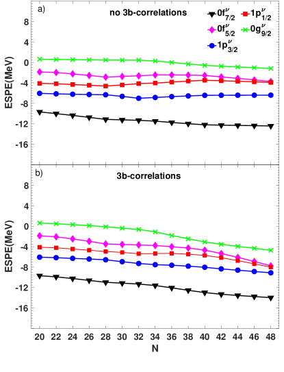
Figure 5: (Color online) ESPE for neutrons in even-even Ti isotopes from $N=20$ to 48 resulting from calculations (a) without and (b) with 3-b correlations.

More interesting is the behavior of the ESPEs for neutrons. Figure 5(a), presenting the neutron ESPEs obtained by omitting 3-b correlations, shows some similarities with Fig. 5(b), where these correlations are included. In both calculations, the neutron $0f_{7/2}$ orbital is well isolated from the others along all the isotopic chain, and a fairly large spacing is observed between the $1p_{3/2}$ and $1p_{1/2}$ orbitals up to $N=44$, which gives rise to the subshell closure at $N=28$ and $N=32$, respectively. No shell closure is instead predicted at $N=34$, corresponding to the filling of the $1p^{\nu}_{1/2}$ orbital, whose separation energy from the $0f^{\nu}_{5/2}$ orbital decreases with increasing neutron number. In spite of these similarities, however, we note that 3-b correlations introduce appreciable changes in the neutron ESPEs, which explain the differences in the two-neutron separation energies and in the $2^{+}_{1}$ excitation energies discussed above. In particular, we see that all the neutron ESPEs show a more rapid and almost continuous decrease as a function of $N$ when 3-b correlations are taken into account, while the neglect of these correlations leads to a more flat behavior or even to an increasing trend for the $1p^{\nu}_{3/2}$, $1p^{\nu}_{1/2}$, and $0f^{\nu}_{5/2}$ orbitals from $N=30$ or $34$ to 40. This explains the strong negative slope of the $S_{2n}$ curve when calculations are performed without including 3-b correlations. Moreover, the $0g^{\nu}_{9/2}-0f^{\nu}_{5/2}$ gap is affected by 3-b correlations which reduce its value by $\approx 400$ keV at $N=40$. The larger gap we find when 3-b correlations are neglected leads to the increase in energy of the $2^{+}_{1}$ state from ⁶⁰Ti to ⁶²Ti we predict in such a case.

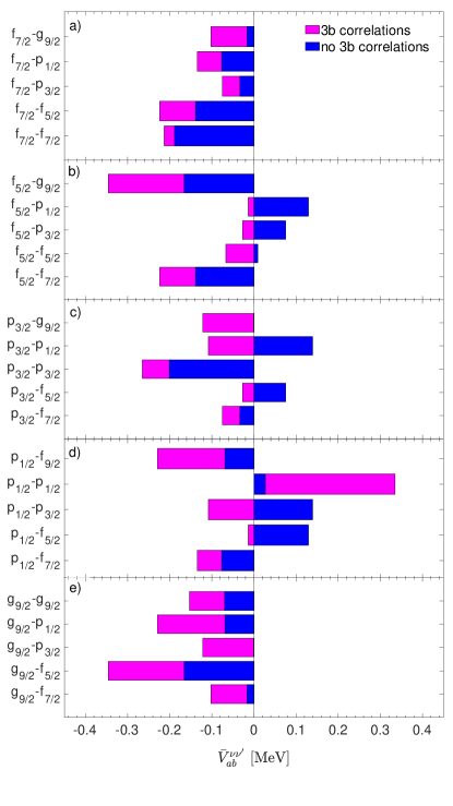
Figure 6: (Color online) Neutron-neutron monopole matrix elements, ${\bar{V}}^{\nu\nu^{\prime}}_{ab}$, of the effective interactions with and without 3-b correlations (see text for details).

The different behavior of the neutron ESPEs with and without 3-b correlations is related to the changes these correlations produce in the monopole part of the neutron-neutron interaction. Actually, the neutron-proton monopole components, which also enter in the neutron ESPE definition, are not significantly affected by 3-b correlations, and, additionally, they do not play a relevant role since their contribution is limited by the reduced number of valence protons. As concerns the neutron-neutron monopole components, we find that 3-b correlations induce on the overall a larger attractiveness which explains the difference in the behavior of the neutron ESPEs shown in Figs. 5(a) and 5(b). As an example, we compare in Fig. 6 the monopole matrix elements of the neutron-neutron effective interaction without 3-b correlations with those of the density-dependent interaction at $N=40$. It can be seen that the only matrix element that acquire a repulsive component is ${\bar{V}}_{1p_{1/2}1p_{1/2}}^{\nu\nu}$.

Furthermore, the size of changes induced by 3-b correlations is orbital dependent, which leads to modifications of the ESPE spacings. In particular, ${\bar{V}}_{0g_{9/2}b}^{\nu\nu}$ receive a larger attractive contribution with respect to ${\bar{V}}_{0f_{5/2}b}^{\nu\nu}$ for any value of $b$, except for $b=0g_{9/2}$. This gives rise to the reduced gap between the $0_{9/2}$ and $0f_{5/2}$ ESPEs we find at $N=40$ when 3-b correlations are taken into account.

To better asses the role of the monopole contributions arising from 3-b correlations we have investigated the interplay of monopole and multipole components. To this end, we have built a modified effective interaction for each Ti isotope starting from the Hamiltonian without 3-b correlations and replacing its monopole component with that arising from the density-dependent Hamiltonian derived for the same nucleus. The obtained results are very close to those of the original density-dependent Hamiltonians, showing, in particular, that the behavior of the two-neutron separation energies and of the $2^{+}_{1}$ excitation energies is essentially determined by the monopole component.

IV Summary and conclusions

In this paper we have studied the even-even Ti isotopic chain from $A=42$ to 70 within the realistic SM framework starting from up-to-date two- and three-body forces derived from ChPT. The one and two-body matrix components of the SM effective Hamiltonian are derived by means of the many-body perturbation in a model space spanned by the proton and neutron $0f1p$ orbitals plus the neutron $0g_{9/2}$ orbital. Three-body contributions are also included through density-dependent TBME consistently derived within a microscopic approach from chiral forces. These correlations are essential to account for the Pauli blocking effect due to the progressive filling of the model space orbitals in nuclei with more than two valence nucleons.

As in our previous paper Coraggio et al. (2020), we have compared the calculated two-neutron separation energies and the excitation energies of the yrast $2^{+}$ state with the available experimental data.

We have found that 3-b correlations have a tiny impact on the two-neutron separation energies up to $N=32$ but, starting from $N=34$ on, their role becomes more relevant with the increasing number of valence neutrons. This results in an upshift of the two-neutron separation energies that become very close to the experimental ones up ⁶²Ti beyond which no experimental information is available. This makes us confident in our predictions for the heaviest Ti isotopes, which we found to be bound up to $N=70$. In Ref. Coraggio et al. (2020), we have shown that 3-b correlations are relevant also to determine the drip line in Ca isotopes. In fact, without the inclusions of these correlations the drip line of calcium isotopes is located at $N=40$, while their attractive contribution shifts the last bound nucleus at least to ⁶⁸Ca.

As concerns the excitation energies of the yrast $2^{+}$ states, we do not obtain a satisfactory agreement with experiment from $N=36$ on, despite the inclusion of 3-b correlations. As a matter of fact, the decreasing trend observed from $N=36$ to $40$ is not reproduced even if correlations are taken into account. This may be related to the omission of the neutron $1d_{5/2}$ orbital, which, as discussed above, is fundamental to reproduce the collectivity of nuclei ”north-east” of ⁴⁸Ca around a $N=40$, especially of ⁶⁴Cr and ⁶²Fe. Nevertheless, our calculations evince that contributions arising from 3-b correlations affect the neutron-neutron monopole components leading to a reduction of the excitation energy of the $2^{+}_{1}$ state and in particular of the shell gap at ⁶²Ti. A similar result was found for the excitation energy of $2^{+}_{1}$ state in ⁶⁰Ca, whose value is reduced by their inclusion from $\sim 2.3$ to 1.7 MeV, which is quite small when compared with the gaps observed in ⁵²Ca and ⁴⁸Ca, namely $\approx 2.5$ and $\approx 4.0$ MeV.

Despite the missing contribution coming from the neutron $1d_{5/2}$ orbital, interesting conclusions can be drawn. In fact, the present study shows that starting from $N=34$ the attractive contribution arising from 3-b correlations impacts significantly on the shell structure evolution.

We plan in a near future to overcome the computational complexity related to the large model by including the neutron $1d_{5/2}$ orbital so as to perform large-scale SM calculations to study the collective behavior at $N=40$ starting from chiral two- and three-body forces and employing single-particle energies and two-body matrix elements derived from many-body perturbation theory.