A unification of least-squares and Green-Gauss gradients under a common projection-based gradient reconstruction framework

Abstract

We propose a family of gradient reconstruction schemes based on the solution of over-determined systems by orthogonal or oblique projections. In the case of orthogonal projections, we retrieve familiar weighted least-squares gradients, but we also propose new direction-weighted variants. On the other hand, using oblique projections that employ cell face normal vectors we derive variations of consistent Green-Gauss gradients, which we call Taylor-Gauss gradients. The gradients are tested and compared on a variety of grids such as structured, locally refined, randomly perturbed, unstructured, and with high aspect ratio. The tests include quadrilateral and triangular grids, and employ both compact and extended stencils, and observations are made about the best choice of gradient and weighting scheme for each case. On high aspect ratio grids, it is found that most gradients can exhibit a kind of numerical instability that may be so severe as to make the gradient unusable. A theoretical analysis of the instability reveals that it is triggered by roundoff errors in the calculation of the cell centroids, but ultimately is due to truncation errors of the gradient reconstruction scheme, rather than roundoff errors. Based on this analysis, we provide guidelines on the range of weights that can be used safely with least squares methods to avoid this instability.

[1]organization=Department of Mechanical and Manufacturing Engineering, University of Cyprus, addressline=P.O. Box 20537, city=Nicosia, postcode=1678, state=, country=Cyprus

[2]organization=Engys, addressline=Studio 20, Royal Victoria Patriotic Building, John Archer Way, city=London, postcode=SW18 3SX, state=, country=U.K.

[3]organization=Laboratory of Fluid Mechanics and Rheology, Dept. of Chemical Engineering, University of Patras, addressline=, city=Patras, postcode=26500, state=, country=Greece

1 Introduction

Gradient reconstruction schemes are among the fundamental ingredients of Finite Volume Methods (FVMs). They are used in the discretisation of diffusion [1, 2] and convection [3] terms, of terms of turbulence closure equations [4], of terms of non-Newtonian constitutive equations [5, 3, 6, 7] etc. Although lately a significant amount of research has gone into the development of high-order FVMs, the second-order accurate FVMs continue to be the most popular choice, due to ease of implementation, low memory requirements, faster execution (for the same number of degrees of freedom), better understanding and familiarity with the discretisation and stabilisation schemes etc. For such reasons, low-order methods will likely remain a popular choice in the foreseeable future (and this holds true even for finite element methods [8, 9], for which achievement of high-order accuracy is relatively more straightforward than for FVMs). For second-order accurate FVMs, the main families of gradient schemes in use are the Green-Gauss (GG) gradients [10, 11, 12, 4, 13, 14], which are derived from the divergence (Gauss) theorem, and the least-squares (LS) gradients [15, 16, 17, 18, 13, 14], which are derived from least-squares error minimisation (the latter are also easily applicable to high-order FVMs). The performance of each gradient scheme depends on the geometrical characteristics of the grid and on the function being differentiated.

In a previous publication [19] we analysed the properties of both of these gradient families, and showed in theory and verified in practice that the GG gradients require special grid smoothness in order to be consistent, whereas LS gradients are always at least first-order accurate, which is a prerequisite for a second-order accurate FVM on grids of general geometry. Despite their shortcomings, GG gradients remain popular and a number of recent publications have addressed the problem of their inconsistency [20, 21, 22, 23, 24]. One way to remove the inconsistency is through an iterative procedure that couples the gradients at neighbouring grid cells [25, 13, 19, 21, 22] (equivalently, a large linear system that includes the gradients at all grid cells can be solved [26]). This procedure is expensive, but if the gradient iterations are interwoven with the solution iterations of an implicit FVM then the gradient computation cost becomes almost as small as for the uniterated GG gradient [19, 21]. Another option for obtaining consistent GG gradient schemes, without the need for iteration, is to apply the Gauss theorem to suitably selected auxiliary cells rather than to the actual grid cells [19, 24].

The aforementioned GG gradient variants achieve consistency at a price, which is either the need for iterations or large linear system solving, or the additional complexity of constructing the auxiliary cells, which can be significant for three-dimensional grids of general topology. However, there does exist another GG gradient variant, named “quasi-Green” (QG) gradient by its inventors, which is consistent but avoids these additional costs [27, 28]; it achieves this by a form of self-correction. Although not new, the QG gradient seems to have gone mostly unnoticed. The QG gradient is of particular interest in the present study because it turns out to be identical with a particular member of a new family of gradient schemes whose derivation is related to that of the least-squares gradients.

The other major family of gradient schemes is that based on least-squares minimisation. The least-squares gradients have no inconsistency, being at least first-order accurate always [19]. In the past they acquired a reputation of producing large errors on curved geometries gridded with cells of very high aspect ratio [29], but proper inverse-distance weighting overcomes the problem in many cases [29, 30]. Nevertheless, in some cases the only way to improve the accuracy is to extend the least-squares computational stencil beyond the immediate neighbours of the cell, notably on grids of triangles (or tetrahedra) where some spatial directions are under-represented by the nearest-neighbour stencils. On such grids, augmented-stencil LS gradients were found in [30] to outperform GG gradients, the latter being made consistent by application of corrections calculated with the aid of LS gradients. Stencil augmentation is not straightforward when it comes to GG gradients and has not been applied, to the best of our knowledge.

In a previous (not peer-reviewed) work [31] we proposed a new family of consistent gradient methods, with similarities to both the GG and LS gradients, which we called “Taylor-Gauss” (TG) gradients. The starting point of the derivation of the TG gradients is the same as for the LS gradients, namely the Taylor series expansion of the values of the function, whose gradient is sought, at neighbour cell centres. This results in an overdetermined system for the gradient, which in the LS case is solved via an orthogonal projection. In the TG case, it is solved by an oblique projection, whose direction is determined by the vectors normal to the cell faces – hence the resemblance to the GG gradient. Therefore, the LS and TG gradients are members of a larger family of gradient schemes which express the differentiated variable at neighbour cell centres in terms of Taylor series and solve the resulting overdetermined system via some sort of projection. Furthermore, after the publication of [31], it has been realised that one of the basic members of the TG family can be recast as the QG gradient mentioned above. This provides an interesting link between least-squares and Green-Gauss gradients.

The present paper aims to present a unified discussion of, and comparison between, the TG, LS, and QG gradients. This encompasses the larger part of available schemes for FVMs, as the majority of FVM gradient schemes currently in use belong either to the LS family or to the GG family (the latter represented here by the QG gradient). The TG gradients constitute the link between the LS and GG gradients, as they can be viewed either as a projection method, like the LS gradients, or as a family of QG gradients, as will be shown. This theoretical unification of the various gradients provides deeper insight that can help to advance the field.

The paper begins in Sec. 2 with a presentation of the general framework for formulating gradient schemes whereby the differentiated variable is expanded in Taylor series in the neighbourhood of the cell in question and the resulting overdetermined system is solved via some projection. Particular projections that lead to the least-squares and Taylor-Gauss gradients are described in Sections 3 and 4, respectively. Several variants of these methods are described, that correspond to different choices of weighting scheme. Subsequently, in Sec. 5, the Taylor-Gauss gradients are re-derived as self-corrected Green-Gauss gradients. The theory is followed by numerical tests on grids of various topologies in Sec. 7, which verify the theoretical orders of accuracy of the schemes. In Section 8, the gradients are tested on the aforementioned challenging case that combines a curved geometry and a very high aspect ratio grid. This case brings to the surface issues of numerical stability, in addition to accuracy. In particular, it is observed that, as the grid is refined, eventually errors related to finite precision arithmetic can become important, depending on the weighting scheme. The paper concludes in Sec. 9.

The scope of the present work is limited to the standalone accuracy of the gradient schemes themselves, i.e. their ability to compute the gradient of a function. Although there are applications for which this knowledge suffices, e.g. [32], in the majority of applications the gradient schemes would be part of an overall composite discretisation scheme used to solve a set of differential equations – a finite volume method. The effect of the gradient scheme on the discretisation error of a FVM is complex and not determined solely by the accuracy of the gradient scheme per se. A study of the latter, however, which is the topic of the present paper, is a prerequisite for obtaining a more complete understanding of the former. We also note that all of the presently examined gradient schemes are “explicit” in the sense that they compute the gradient using only the values of the differentiated variable at nearby cell centres. As mentioned, there exist also “implicit” gradient schemes where the gradient at a cell depends additionally on the gradients at nearby cells; hence these schemes require iteration or solution of domain-wide linear systems. Given the much higher computational cost of the implicit gradients, they do not appear to be advantageous compared to explicit gradients if all that is required is to compute the gradient of a function. However, it is possible that they have advantages when used as a component of a FVM, e.g. they may offer better stability or iterative convergence. The effect of the choice of gradient scheme on the FVM solution deserves a separate study, which we plan for the future, on a variety of continuum mechanics problems.

It is also noted that all of the presented gradient schemes are formally of first-order accuracy (in practice they are second-order accurate on smooth grids); thus they can serve as components of second-order accurate FVMs. Least-squares gradients are straightforward to extend to higher-order accuracy (see e.g. [17, 33]), but not so for gradients that employ face normal vectors (TG and GG gradients). Finally, to keep things simple, the present work is limited to two-dimensional geometries.

2 General framework: Taylor expansion and projection

Suppose we wish to calculate the gradient of a function $\phi$ at the centre $\underline{C}_{0}$ of a cell under consideration (Fig. 1). Let us first introduce some definitions and notation. The cell has $F$ faces, each of which either separates it from a single neighbour cell, or is a boundary face. We will use a local indexing system where index 0 is assigned to the cell where the gradient is sought, and indices $f>0$ are assigned to nearby cells involved in the calculation. For $f\leq F$, index $f$ is assigned to the neighbour cell that shares face $f$. The centroids of these cells are denoted as $\underline{C}_{0}$ and $\underline{C}_{f}$, respectively (geometric vectors are denoted with an underline). If face $f$ is a boundary face then its centroid $\underline{c}_{f}$ will be used instead, assuming the value of $\phi$ is known there. Gradient schemes will reconstruct the gradient at $\underline{C}_{0}$ from the values of $\phi$ at $\underline{C}_{0}$ and at $N$ additional points, where $N=F$ for nearest-neighbour schemes and $N>F$ for extended-stencil schemes. Using only the nearest neighbours allows an implementation that uses simpler data structures; however, sometimes these points do not carry sufficient information and additional points are needed. Some of the gradient schemes examined here, namely the least-squares schemes, can use any set of neighbour points, but others, namely those making use of the cell’s faces such as the Green-Gauss gradient, are limited to nearest neighbours only, and cannot be extended to additional points in a straightforward manner.

Some geometric definitions are as follows. An interior face $f$ has centroid $\underline{c}_{f}$, whose projection on the line joining $\underline{C}_{0}$ and $\underline{C}_{f}$ is denoted as $\underline{c}^{\prime}_{f}$. The point $\underline{m}_{f}=(\underline{C}_{0}+\underline{C}_{f})/2$ lies midway between $\underline{C}_{0}$ and $\underline{C}_{f}$. The distance vector from $\underline{C}_{0}$ to $\underline{C}_{f}$ is denoted as $\underline{D}_{f}=\underline{C}_{f}-\underline{C}_{0}$, and the unit vector in the same direction as $\hat{\underline{d}}=\underline{D}_{f}/\|\underline{D}_{f}\|$. The unit vector normal to face $f$ is denoted by $\hat{\underline{s}}_{f}$, and if we multiply this by the face area $S_{f}$ we get the face vector $\underline{S}_{f}=S_{f}\hat{\underline{s}}_{f}$. We can define the following important grid quality metrics [19]: Skewness is the deviation of the centroid $\underline{c}_{f}$ from the line joining $\underline{C}$ and $\underline{C}_{f}$, and can be quantified as $\|\underline{c}_{f}-\underline{c}^{\prime}_{f}\|/\|\underline{D}_{f}\|$; non-orthogonality is the angle between $\hat{\underline{d}}_{f}$ and $\hat{\underline{s}}_{f}$; and unevenness is the asymmetrical distancing of points $\underline{C}$ and $\underline{C}_{f}$ from face $f$, which can be quantified as $\|\underline{c}^{\prime}_{f}-\underline{m}_{f}\|/\|\underline{D}_{f}\|$.

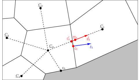
Figure 1: The notation adopted in the present paper (see text for details).

Eventually, the reconstruction scheme must involve only values of $\phi$ at cell centres, but in a first step we can express $\phi$ in terms of Taylor series at a number of points $\underline{P}_{1},\underline{P}_{2},\ldots,\underline{P}_{N}$ that are not necessarily the cell centroids. If the points $\underline{P}_{f}$ are different from $\underline{C}_{f}$ then a further step is required where the (approximate) values $\phi(\underline{P}_{i})$ are interpolated from the values $\phi(\underline{C}_{j})$. In any case, the change of $\phi$ between $\underline{C}_{0}$ and the points $\underline{P}_{f}$, $\Delta\phi_{f}=\phi(\underline{P}_{f})-\phi(\underline{C}_{0})$, is given by (using Taylor series):

$$\Delta\phi_{f}\;=\;\underline{R}_{f}\cdot\nabla\phi(\underline{C}_{0})\;+\;\frac{1}{2}\underline{R}_{f}\underline{R}_{f}:\nabla\nabla\phi(\underline{C}_{0})\;+\;O(h^{3})$$ (1)

where $\underline{R}_{f}=\underline{P}_{f}-\underline{C}_{0}$, and $h$ is a typical cell dimension. Vectors written next to each other, such as $\underline{R}_{f}\underline{R}_{f}$ above, denotes the tensor product.

If we drop the second- and higher-order terms of the above equations, then we are left with $N$ equations with D=2 or D=3 unknowns (the components of $\nabla\phi(\underline{C}_{0})$), in two or three dimensional space, respectively. Thus we have an over-determined system with no solution. From it, we can obtain a full-rank D$\times$D system with unique solution by the following procedure. We first weigh (left-multiply) each equation (1) by a vector $\underline{V}_{f}$ (the choice of vector will be discussed later), to convert it into a vector equation:

$$\underline{V}_{f}\Delta\phi_{f}\;=\;\underline{V}_{f}\underline{R}_{f}\cdot\nabla\phi(\underline{C}_{0})\;+\;\frac{1}{2}\underline{V}_{f}\underline{R}_{f}\underline{R}_{f}:\nabla\nabla\phi(\underline{C}_{0})\;+\;O(\underline{V}_{f})\cdot O(h^{3})$$ (2)

Then, we sum all of the equations (2):

$$\sum_{f}\underline{V}_{f}\Delta\phi_{f}\;=\;\left[\sum_{f}\underline{V}_{f}\underline{R}_{f}\right]\cdot\nabla\phi(\underline{C}_{0})\;+\;\frac{1}{2}\left[\sum_{f}\underline{V}_{f}\underline{R}_{f}\underline{R}_{f}\right]:\nabla\nabla\phi(\underline{C}_{0})\;+\;O(\underline{V}_{f})\cdot O(h^{3})$$ (3)

Because $\underline{R}_{f}=O(h)$, we have $\underline{V}_{f}\underline{R}_{f}\underline{R}_{f}=O(\underline{V}_{f})\cdot O(h^{2})$. Grouping together all terms of order 2 or higher and solving for $\nabla\phi(\underline{C}_{0})$ we obtain

$$\nabla\phi(\underline{C}_{0})\;=\;\left[\sum_{f}\underline{V}_{f}\underline{R}_{f}\right]^{-1}\!\cdot\left[\sum_{f}\underline{V}_{f}\Delta\phi_{f}\right]\;+\;\underbrace{\left[\sum_{f}\underline{V}_{f}\underline{R}_{f}\right]^{-1}\!\cdot O(\underline{V}_{f})\cdot O(h^{2})}_{=\;[O(\underline{V}_{f})O(h)]^{-1}\cdot O(\underline{V}_{f})O(h^{2})\;=\;O(h)}$$ (4)

or, summarising:

$$\nabla\phi(\underline{C}_{0})\;=\;\left[\sum_{f}\underline{V}_{f}\underline{R}_{f}\right]^{-1}\!\cdot\left[\sum_{f}\underline{V}_{f}\Delta\phi_{f}\right]\;+\;O(h)$$ (5)

We have thus arrived at a gradient scheme that is at least first-order accurate (it is also exact for linear functions, as can be seen from Eq. (3), where in the case of a linear function $\nabla\nabla\phi$ and all the higher derivatives are zero), and therefore appropriate for second-order accurate FVMs [19]. It must be noted that this analysis assumes that the values $\Delta\phi_{f}$ are exact, which will be the case if the points $\underline{P}_{f}$ are cell centroids, $\underline{C}_{f}$. If not, then the interpolation used to obtain approximate values $\tilde{\phi}(\underline{P}_{f})=\phi(\underline{P}_{f})+O(h^{p})$, where $p$ is the order of interpolation, will introduce additional errors. In this case, the exact differences $\Delta\phi_{f}$ will not be available to us, but rather approximate values $\Delta\tilde{\phi}_{f}=\Delta\phi_{f}+O(h^{p})$. Substituting in (5) we obtain:

$$\nabla\phi(\underline{C}_{0})\;=\;\left[\sum_{f}\underline{V}_{f}\underline{R}_{f}\right]^{-1}\!\cdot\left[\sum_{f}\underline{V}_{f}\Delta\tilde{\phi}_{f}\right]\;+\;\underbrace{\left[\sum_{f}\underline{V}_{f}\underline{R}_{f}\right]^{-1}\!\cdot\left[\sum_{f}\underline{V}_{f}O(h^{p})\right]}_{=\;[O(\underline{V}_{f})O(h)]^{-1}\cdot O(\underline{V}_{f})O(h^{p})\;=\;O(h^{p-1})}\;+\;O(h)$$ (6)

Therefore, the order of accuracy of the gradient in this case is $\min\{p-1,\,1\}$. In order to have a gradient that is at least first-order accurate, the order of interpolation must be $p\geq 2$. This makes good candidates for points $\underline{P}_{f}$ the points that lie on the lines joining $\underline{C}_{0}$ to $\underline{C}_{f}$, such as $\underline{c}^{\prime}_{f}$ and $\underline{m}_{f}$, as $\phi$ can be obtained there with linear interpolation ($p=2$).

It is noteworthy that, to this point, we have particularised neither the weighting vectors $\underline{V}_{f}$ (possible choices include $\underline{R}_{f}$, $\hat{\underline{d}}_{f}$, $\underline{D}_{f}$ $\hat{\underline{s}_{f}}$, $\underline{S}_{f}$, and many others), nor the points $\underline{P}_{f}$ (and therefore the vectors $\underline{R}_{f}$ appearing in (5)). The scheme (5) is, therefore, quite general. Despite appearing as something new, it will soon be shown that very familiar gradient schemes, such as least-squares gradients and a self-corrected variation of the Green-Gauss gradient, can be cast in this form.

The scheme (5) is very general, but nevertheless there are some minimal restrictions on the vectors $\underline{R}_{f}$ and $\underline{V}_{f}$ involved in the calculation. In order for the D$\times$D matrix $\sum_{f}\underline{V}_{f}\underline{R}_{f}$ to be invertible, it must be of full rank, i.e. it must have linearly independent columns (and linearly independent rows). Obviously each of the component matrices $\underline{V}_{f}\underline{R}_{f}$ has rank 1 and is singular, but their sum may be of full rank. The columns of $\sum_{f}\underline{V}_{f}\underline{R}_{f}$ are linear combinations of the vectors $\underline{V}_{f}$, and therefore we need at least D linearly independent vectors $\underline{V}_{f}$ (in fact we can’t have more than D in D-dimensional space). Similarly, for $\sum_{f}\underline{V}_{f}\underline{R}_{f}$ to have D linearly independent rows we need D linearly independent direction vectors $\underline{R}_{f}$. These requirements are hardly surprising.

2.1 Some linear algebra

Before discussing particular instances of the general scheme (5) it is useful to take another look at it from a linear algebra perspective. In matrix form, the over-determined system (1), after dropping the second- and higher-order terms, is (for simplicity the two-dimensional case is assumed):

$$\begin{bmatrix}R_{1,x}&R_{1,y}\\ R_{2,x}&R_{2,y}\\ \vdots&\vdots\\ R_{N,x}&R_{N,y}\end{bmatrix}\cdot\begin{bmatrix}\phi_{.x}\\ \phi_{.y}\end{bmatrix}\;=\;\begin{bmatrix}\Delta\phi_{1}\\ \Delta\phi_{2}\\ \vdots\\ \Delta\phi_{N}\end{bmatrix}$$ (7)

where $\underline{R}_{f}=(R_{f,x},R_{f,y})$ and $\nabla\phi(\underline{C}_{0})=(\phi_{.x},\phi_{.y})$ in Cartesian component form. We can write this in compact matrix notation as

$$\mathbf{Rx}=\mathbf{b}$$ (8)

where $\mathbf{R}$ is $N\times 2$, $\mathbf{x}$ is $2\times 1$ and contains the sought derivatives, and $\mathbf{b}$ is $N\times 1$. To turn this into a solvable $2\times 2$ system, we left-multiply it by the transpose of a full-rank $N\times 2$ matrix $\mathbf{V}$:

$$\mathbf{V}^{\mathrm{T}}\mathbf{Rx}=\mathbf{V}^{\mathrm{T}}\mathbf{b}$$ (9)

This is a $2\times 2$ system which can be solved for $\mathbf{x}$. The solution is:

$$\mathbf{x}\;=\;(\mathbf{V}^{\mathrm{T}}\mathbf{R})^{-1}\mathbf{V}^{\mathrm{T}}\mathbf{b}$$ (10)

A little contemplation reveals that Eq. (9) is equivalent to (2) (if we omit the higher-order terms), and Eq. (10) is equivalent to Eq. (5); the rows of the matrix $\mathbf{V}$ are the vectors $\underline{V}_{f}$.

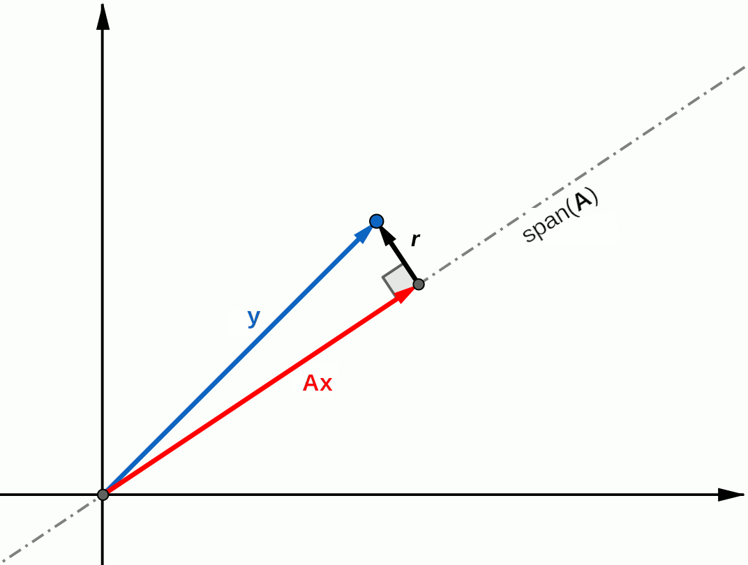
(a) Orthogonal projection

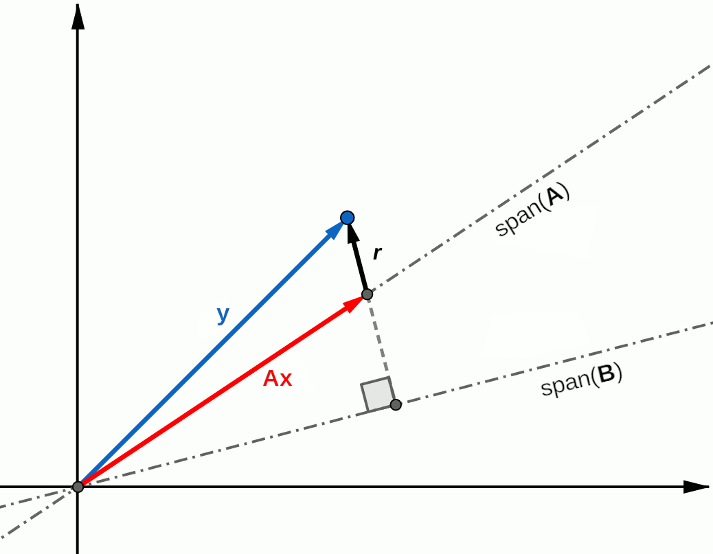
(b) Oblique projection

Figure 2: Orthogonal 2(a) and oblique 2(b) projections $\mathbf{Ax}$ of the vector $\mathbf{y}$ onto the subspace $\mathrm{span}(\mathbf{A})$. The difference $\mathbf{r}=\mathbf{y}-\mathbf{Ax}$ is orthogonal to either $\mathrm{span}(\mathbf{A})$ 2(a) or to another subspace $\mathrm{span}(\mathbf{B})$ 2(b).

We know from linear algebra (e.g. [34]) that if $\mathbf{Ax}=\mathbf{y}$ is an overdetermined system then the solution $\mathbf{x}$ that minimises the L2 norm of the error $\mathbf{r}=\mathbf{y}-\mathbf{Ax}$ satisfies

$$\mathbf{A}^{\mathrm{T}}(\mathbf{y}-\mathbf{Ax})\;=\;\mathbf{0}$$ (11)

In this case, the error $\mathbf{r}$ is orthogonal to the column space of $\mathbf{A}$ and $\mathbf{Ax}$ is the orthogonal projection of $\mathbf{y}$ onto $\mathrm{span}(\mathbf{A})$. However, we could instead choose $\mathbf{x}$ such that $\mathbf{r}=\mathbf{y}-\mathbf{Ax}$ is orthogonal to another subspace, spanned by the columns of a matrix $\mathbf{B}$, in which case $\mathbf{Ax}$ is an oblique projection of $\mathbf{y}$ onto $\mathrm{span}(\mathbf{A})$:

$$\mathbf{B}^{\mathrm{T}}(\mathbf{y}-\mathbf{Ax})\;=\;\mathbf{0}$$ (12)

These cases are illustrated in Fig. 2. Equation (9) is of the form (12), but sometimes can be cast in the form (11) which is preferable from a theoretical standpoint because it allows us to discern a quantity that is minimised by the gradient scheme. Choices of $\mathbf{V}$ that allow this are, for example:

• $\mathbf{V}=\mathbf{R}$. Equation (9) can be rearranged in the form (11) as $\mathbf{R}^{\mathrm{T}}(\mathbf{b}-\mathbf{Rx})=\mathbf{0}$, whose solution $\mathbf{x}$ minimises $\|\mathbf{b}-\mathbf{Rx}\|_{2}$. This is the unweighted least squares method.

• $\mathbf{V}=\mathbf{DR}$, where $\mathbf{D}$ is a diagonal matrix. Equation (9) can be recast in the form (11) as $(\mathbf{D}^{\frac{1}{2}}\mathbf{R})^{\mathrm{T}}(\mathbf{D}^{\frac{1}{2}}\mathbf{b}-\mathbf{D}^{\frac{1}{2}}\mathbf{Rx})=\mathbf{0}$. The quantity minimised is $\|\mathbf{D}^{\frac{1}{2}}\mathbf{b}-\mathbf{D}^{\frac{1}{2}}\mathbf{Rx}\|_{2}=\|\mathbf{D}^{\frac{1}{2}}(\mathbf{b}-\mathbf{Rx})\|_{2}$. So, it is again the magnitude of the discrepancy array $\mathbf{r}=\mathbf{b}-\mathbf{Rx}$ that is minimised, but this time not all components carry equal weight; the weights are stored in $\mathbf{D}^{\frac{1}{2}}$. Usually, components that come from farther neighbours carry less weight. Weighted least-squares gradients have this form.

• $\mathbf{V}=\mathbf{W}^{\mathrm{T}}\mathbf{WR}$, where $\mathbf{W}$ is a full matrix. This is the natural generalisation of the previous case: Eq. (9) can be cast as $(\mathbf{W}\mathbf{R})^{\mathrm{T}}(\mathbf{W}\mathbf{b}-\mathbf{W}\mathbf{Rx})=\mathbf{0}$, and the norm of $\mathbf{W}(\mathbf{b}-\mathbf{Rx})$ is minimised.

3 Least-squares gradients

Least-squares gradients are those that can be cast in the form (11). Here we will list a few particular schemes resulting from particular choices of the weights (matrix $\mathbf{D}$; full weight matrices $\mathbf{W}$, although offering more control, will not be examined here) – one of these schemes is new, to the best of our knowledge. Least squares gradients usually employ the cell centroids $\underline{C}_{f}$ as the points $\underline{P}_{f}$, avoiding any interpolation, which is the practice followed here as well.

3.1 Unweighted least-squares

The unweighted least-squares gradient is the scheme that comes from setting $\underline{V}_{f}=\underline{R}_{f}$ in Eq. (5), or $\mathbf{V}=\mathbf{R}$ in (10). It minimises the sum $\sum_{f}(\Delta\phi_{f}-\underline{R}_{f}\cdot\tilde{\nabla}(\underline{C}_{0}))^{2}$ (where $\tilde{\nabla}$ denotes the approximate gradient). This sum can also be written as

$$\sum_{f}\left[\|\underline{R}_{f}\|\left(\frac{\Delta\phi_{f}}{\|\underline{R}_{f}\|}\;-\;\hat{\underline{d}}_{f}\cdot\tilde{\nabla}\phi(\underline{C}_{0})\right)\right]^{2}$$ (13)

Thus although “unweighted”, this scheme preferentially tries to minimise the difference between the approximation of the directional derivative, $\hat{\underline{d}}_{f}\cdot\tilde{\nabla}(\underline{C}_{0})$, and the finite difference approximation of that derivative, $\Delta\phi_{f}/\|\underline{R}_{f}\|$, mostly in the directions $f$ of more distant neighbours (larger $\|\underline{R}_{f}\|$). This is unnatural, as normally one would want to assign equal weights to the directional derivatives in all directions, or even to assign larger weights to the directions of closer neighbours, since the closer we are to $\underline{C}_{0}$ the more linearly $\phi$ varies. Therefore it is not surprising that this scheme often performs poorly, and that inverse-distance-weighted least squares schemes are more popular.

3.2 Inverse-distance-weighted least-squares

To remedy the aforementioned problem, the weight vectors $\underline{V}_{f}$ can instead be defined as

$$\underline{V}_{f}\;=\;\frac{1}{\|\underline{R}_{f}\|^{q}}\,\underline{R}_{f}$$ (14)

where $q$ is an exponent usually in the range $q\in[0,4]$ ($q=0$ corresponds to the unweighted least squares gradient of Sec. 3.1). For brevity, henceforth the scheme with weights (14) will be denoted as the LS($q$) gradient.

3.3 Area-weighted least-squares

Inverse-distance-weighting accounts for the fact that the neighbour points $\underline{P}_{f}$ may not be equidistant from $\underline{C}_{0}$. Another factor that may cause the performance of the gradient to suffer is that the points $\underline{P}_{f}$ may not be distributed equally in all directions around $\underline{C}_{0}$. In [19] it was shown that when some points are clustered in a particular direction, the scheme (14) may not achieve optimal accuracy because this direction is over-represented in the calculation.

If only nearest neighbours are included in the calculation, then a possible remedy is to include the face areas as factors in the respective weights:

$$\underline{V}_{f}\;=\;\frac{\|\underline{S}_{f}\|}{\|\underline{R}_{f}\|^{q}}\,\underline{R}_{f}$$ (15)

This is because usually (especially if the grid is orthogonal, $\hat{\underline{d}}_{f}=\hat{\underline{s}}_{f}$) face area is roughly inversely proportional to the degree of clustering in that direction: a large area means that there are no other neighbours around, while a small area means the opposite. This is not completely accurate, but it is easy to implement as the face areas $\|\underline{S}_{f}\|$ are readily available. Henceforth we will refer to this scheme as LSA($q$) gradient.

3.4 Direction-weighted least-squares

A more diligent quantification of the degree of clustering in each direction is the following. We define

$$\theta_{ij}\;=\;\theta_{ji}\;=\;\begin{dcases}\hat{\underline{d}}_{i}\cdot\hat{\underline{d}}_{j}&\quad\text{if}\;\;\;\hat{\underline{d}}_{i}\cdot\hat{\underline{d}}_{j}\geq 0\\ 0&\quad\text{if}\;\;\;\hat{\underline{d}}_{i}\cdot\hat{\underline{d}}_{j}<0\end{dcases}$$ (16)

$\theta_{ij}$ is a measure of the alignment of directions $\hat{\underline{d}}_{i}$ and $\hat{\underline{d}}_{j}$, ranging from 0, if $\hat{\underline{d}}_{i}$ and $\hat{\underline{d}}_{j}$ are perpendicular or point in opposite directions, to 1 if they point in the same direction. Now consider the point $\underline{P}_{f}$, which lies in the direction $\hat{\underline{d}}_{f}$ with respect to $\underline{C}_{0}$. If other points, $\underline{P}_{j}$, are also roughly aligned in the same direction, then the contribution of point $\underline{P}_{f}$ to the computed gradient should be reduced accordingly. One possibility for quantifying this is through the following factor:

$$\Theta_{f}\;=\;\frac{1}{\sum_{j}\theta_{fj}}$$ (17)

This compares the contribution of point $\underline{P}_{f}$ to direction $\hat{\underline{d}}_{f}$ (this contribution is $\theta_{ff}=\hat{\underline{d}}_{f}\cdot\hat{\underline{d}}_{f}=1$, the numerator) to the total contribution from all points (the sum in the denominator). The smaller $\theta_{ff}$ is compared to $\sum_{j}\theta_{fj}$, the less point $\underline{P}_{f}$ should contribute to the gradient.

Therefore, a reasonable choice of weights seems to be:

$$\underline{V}_{f}\;=\;\frac{\Theta_{f}}{\|\underline{R}_{f}\|^{q}}\,\underline{R}_{f}$$ (18)

With this choice, the quantity minimised by the least-squares gradient is:

$$\sum_{f}\left[\left(\frac{\Theta_{f}}{\|\underline{R}_{f}\|^{q}}\right)^{\frac{1}{2}}\|\underline{R}_{f}\|\left(\frac{\Delta\phi_{f}}{\|\underline{R}_{f}\|}\;-\;\hat{\underline{d}}_{f}\cdot\tilde{\nabla}\phi(\underline{C}_{0})\right)\right]^{2}$$ (19)

as follows from the fact that using $\mathbf{V}=\mathbf{DR}$ minimises $\mathbf{D}^{\frac{1}{2}}(\mathbf{b}-\mathbf{Rx})$ (Sec. 2.1).

To ensure that this scheme works reasonably, let us perform a couple of checks. To isolate the effect of directionality, let us assume that all neighbour points $\underline{P}_{f}$ are equidistant from $\underline{C}_{0}$. First, if the points are distributed equally in all directions, then due to symmetry the factors $\Theta_{f}$ will be equal for all points, and all of them will receive equal weight, as is desirable. As another check, consider an extreme case where two points $\underline{P}_{i}$ and $\underline{P}_{j}$ coincide, and none of the other points contribute in that particular direction ($\theta_{ij}=1$ and $\theta_{ik}=0$ for $k\neq i,j$). The reader can verify that the contributions of these two points to the quantity (19) sum up to what would be the contribution of a single point at that location, had there been only one point there.

The scheme (18), henceforth referred to as LSD($q$) gradient, is more expensive than the simpler scheme (15), but has the advantage that the only geometric data it employs are the locations of the points $\underline{P}_{f}$, and thus it does not even require a well-defined grid. This is in line with the popular traditional scheme (14). The LSA scheme (15), on the other hand, requires a well-defined grid with cell faces. The use of the cell faces entails that only nearest neighbours can be involved in the calculation (as for GG gradients). The LSD gradient has no such restriction.

4 Taylor-Gauss gradients

Another option that naturally comes to mind concerning the weight vectors $\underline{V}_{f}$ is to base them on the face area vectors $\underline{S}_{f}$.

$$\underline{V}_{f}\;=\;\frac{1}{\|\underline{R}_{f}\|^{q}}\,\underline{S}_{f}$$ (20)

This scheme, called “Taylor-Gauss” (TG) gradient in [31] is more difficult to analyse from a theoretical perspective because it is an oblique projection scheme and does not perform a task of minimisation. Nevertheless, it will be shown in the next section that it can be interpreted as a consistent form of Green-Gauss gradient. The scheme (20) with the choice $\underline{P}_{f}=\underline{C}_{f}$ will henceforth be referred to as TG($q$) gradient.

Since Green-Gauss gradients typically employ face-centre values of $\phi$, let us briefly examine the implications of choosing the points $\underline{P}_{f}$ to be the points $\underline{c}^{\prime}_{f}$ rather than $\underline{C}_{f}$. It turns out that the resulting scheme is equivalent to that of using the cell centroids $\underline{C}_{f}$ but with altered weights. In particular, for $\underline{P}_{f}=\underline{c}^{\prime}_{f}$ we have $\underline{R}_{f}=\underline{c}^{\prime}_{f}-\underline{C}_{0}$ and $\Delta\phi_{f}=\phi(\underline{c}^{\prime}_{f})-\phi(\underline{C}_{0})$ in Eq. (5), but let us define also $\underline{R}^{*}_{f}=\underline{C}_{f}-\underline{C}_{0}$ and $\Delta\phi^{*}_{f}=\phi(\underline{C}_{f})-\phi(\underline{C}_{0})$ (these are the corresponding values that would be used if we had chosen $\underline{P}_{f}=\underline{C}_{f}$). The value $\phi(\underline{c}^{\prime}_{f})$ is interpolated linearly. If

$$a_{f}\;=\;\frac{\|\underline{c}^{\prime}_{f}-\underline{C}_{0}\|}{\|\underline{C}_{f}-\underline{C}_{0}\|}$$ (21)

is the linear interpolation factor, then $\underline{R}_{f}=a_{f}\underline{R}^{*}_{f}$ and $\Delta\phi_{f}=a_{f}\Delta\phi^{*}_{f}$. Equation (5), with weight vectors (20), can then be written as (omitting the truncation error):

$$\nabla\phi(\underline{C}_{0})\;=\;\left[\sum_{f}\frac{a^{1-q}_{f}}{\|\underline{R}^{*}_{f}\|^{q}}\underline{S}_{f}\underline{R}^{*}_{f}\right]^{-1}\!\cdot\left[\sum_{f}\frac{a^{1-q}_{f}}{\|\underline{R}^{*}_{f}\|^{q}}\underline{S}_{f}\Delta\phi^{*}_{f}\right]$$ (22)

Obviously, the weight vectors in (22) differ from (20) in that they have an extra factor $a^{1-q}_{f}$. So, choosing $\underline{P}_{f}=\underline{c}^{\prime}_{f}$ is equivalent to choosing $\underline{P}_{f}=\underline{C}_{f}$ except that the weight vectors (20) are multiplied by $a^{1-q}_{f}$. We will refer to the scheme (20) with $\underline{P}_{f}=\underline{c}^{\prime}_{f}$ as TGI($q$) gradient (TG with interpolation). For $q=1$, we have $a^{1-q}_{f}=1$ and hence gradients TG(1) and TGI(1) are identical.

5 Self-corrected Green-Gauss gradients

In this section we briefly review the “quasi-Green” (QG) gradient of [27, 28] and show that it is identical to a member of the Taylor-Gauss gradient family. Furthermore, we will show that all members of the TG family can be viewed as self-corrected GG gradients.

The starting point for most Green-Gauss gradients is the following equation, derived from application of the Gauss (divergence) theorem to cell 0 ($\Omega_{0}$ denotes its volume) – see [19] for details of the derivation:

$$\nabla\phi(\underline{C}_{0})\;=\;\frac{1}{\Omega_{0}}\sum_{f}\underline{S}_{f}\phi(\underline{c}_{f})\;+\;O(h)$$ (23)

To proceed further, one must express the values of $\phi$ at the face centroids, $\phi(\underline{c}_{f})$, as a function of the values at the cell centroids $\underline{C}_{i}$, via interpolation. The most popular schemes substitute $\phi(\underline{c}_{f})$ in (23) with the value of $\phi$ at $\underline{c}^{\prime}_{f}$ or at $\underline{m}_{f}$ or at some other point on the line joining $\underline{C}_{0}$ to $\underline{C}_{f}$ where $\phi$ can be linearly interpolated. However, this is only an $O(h)$ approximation to $\phi(\underline{c}_{f})$ and introduces an $O(1)$ error into Eq. (23), making the resulting scheme inconsistent – see [19] for details. Alternatively, a second-order accurate interpolation for $\phi(\underline{c}_{f})$ has been employed:

$$\phi(\underline{c}_{f})\;=\;(1-a_{f})\phi_{0}\;+\;a_{f}\phi_{f}\;+\;(\underline{c}_{f}-\underline{c}^{\prime}_{f})\cdot\nabla\phi(\underline{c}^{\prime}_{f})\;+\;O(h^{2})$$ (24)

where $\phi_{i}=\phi(\underline{C}_{i})$ and $a_{f}$ is the interpolation factor (21) (thus the sum of the first two terms of the right-hand side of (24) is the linearly interpolated value of $\phi$ at point $\underline{c}^{\prime}_{f}$). The gradient in the right-hand side is usually linearly interpolated from the gradients computed at $\underline{C}_{0}$ and $\underline{C}_{f}$. In this case, substituting (24) into (23) results in a consistent GG gradient where the gradient at each cell is coupled to the gradients at all neighbouring cells, thus requiring either iterations [25, 1, 19] or solution of a large linear system [26] to obtain the values of the gradient at all grid cells. This significant computational overhead makes the scheme unattractive.

However, it is not hard to see that linear interpolation for the gradient in (24) is superfluous. Linear interpolation is used for 2nd-order accuracy, but the gradients at $\underline{C}_{0}$ and $\underline{C}_{f}$ are likely only 1st-order accurate anyway. Furthermore, a first-order accurate approximation of the gradient at $\underline{c}^{\prime}_{f}$ is all that is needed in (24) because the $O(h)$ error of the gradient, multiplied by $(\underline{c}_{f}-\underline{c}^{\prime}_{f})$, contributes only a $O(h^{2})$ error to (24). The most convenient 1st-order approximation to $\nabla\phi(\underline{c}^{\prime}_{f})$ is just $\nabla\phi(\underline{C}_{0})$, because this avoids any coupling between the gradients of neighbouring cells. So, replacing $\nabla\phi(\underline{C}_{0})$ for $\nabla\phi(\underline{c}^{\prime}_{f})$ in (24) and substituting the latter expression in (23) gives:

$$\nabla\phi(\underline{C}_{0})\;=\;\frac{1}{\Omega_{0}}\sum_{f}\underline{S}_{f}\left[(1-a_{f})\phi_{0}\;+\;a_{f}\phi_{f}\right]\;+\;\frac{1}{\Omega_{0}}\sum_{f}\underline{S}_{f}(\underline{c}_{f}-\underline{c}^{\prime}_{f})\cdot\nabla\phi(\underline{C}_{0})\;+\;O(h)$$ (25)

which can be solved for the gradient $\nabla\phi(\underline{C}_{0})$ to obtain:

$$\nabla\phi(\underline{C}_{0})\;=\;\frac{1}{\Omega_{0}}\left[\underline{\underline{I}}\;-\;\frac{1}{\Omega_{0}}\sum_{f}\underline{S}_{f}(\underline{c}_{f}-\underline{c}^{\prime}_{f})\right]^{-1}\sum_{f}\underline{S}_{f}\bar{\phi}(\underline{c}^{\prime}_{f})\;+\;O(h)$$ (26)

where $\bar{\phi}(\underline{c}^{\prime}_{f})=(1-a_{f})\phi_{0}+a_{f}\phi_{f}$ is the linearly interpolated value of $\phi$ at $\underline{c}^{\prime}_{f}$, and $\underline{\underline{I}}$ is the identity tensor. It is noted that if $\underline{c}_{f}-\underline{c}^{\prime}_{f}=0$ at all faces then the scheme (26) reduces to the common GG gradient; however, in the presence of skewness ($\underline{c}_{f}-\underline{c}^{\prime}_{f}\neq 0$), the gradient (26) uses its own self (through Eq. (24)) to apply a correction that retains consistency. So, scheme (26) is a self-corrected, consistent, first-order accurate GG gradient. It has been used in [27, 28] where it is termed “quasi-Green” (QG) gradient.

Interestingly, the scheme (26) can be re-written in a familiar form. Consider first the tensor being inverted (in square brackets in (26)). By writing $\underline{c}_{f}-\underline{c}^{\prime}_{f}=(\underline{c}_{f}-\underline{C}_{0})-(\underline{c}^{\prime}_{f}-\underline{C}_{0})$ it can be seen to equal

$$\underline{\underline{I}}\;-\;\frac{1}{\Omega_{0}}\sum_{f}\underline{S}_{f}(\underline{c}_{f}-\underline{c}^{\prime}_{f})\;=\;\underline{\underline{I}}\;-\;\frac{1}{\Omega_{0}}\sum_{f}\underline{S}_{f}(\underline{c}_{f}-\underline{C}_{0})\;+\;\frac{1}{\Omega_{0}}\sum_{f}\underline{S}_{f}(\underline{c}^{\prime}_{f}-\underline{C}_{0})$$ (27)

The second term on the right-hand side happens to equal $\underline{\underline{I}}$, as shown in the Appendix, so it cancels out with the first term. In the remaining term, if we define $\underline{R}_{f}=\underline{C}_{f}-\underline{C}_{0}$, we can express $\underline{c}^{\prime}_{f}-\underline{C}_{0}=a_{f}\underline{R}_{f}$. Finally, we can manipulate the vector multiplied by this inverse tensor in (26) as follows:

$$\sum_{f=1}^{F}\underline{S}_{f}\left[(1-a_{f})\phi_{0}+a_{f}\phi_{f}\right]\;=\;\sum_{f=1}^{F}\underline{S}_{f}\left[\phi_{0}-a_{f}\phi_{0}+a_{f}\phi_{f}\right]\;=\;\phi_{0}\sum_{f=1}^{F}\underline{S}_{f}\;+\;\sum_{f=1}^{F}\underline{S}_{f}a_{f}\Delta\phi_{f}$$ (28)

where $\Delta\phi_{f}=\phi_{f}-\phi_{0}$. The first term of the right-hand side of (28) is zero because $\sum_{f}\underline{S}_{f}=\underline{0}$.

Putting everything together, the QG gradient (26) can also be expressed as

$$\nabla\phi(\underline{C}_{0})\;=\;\left[\sum_{f}a_{f}\underline{S}_{f}\underline{R}_{f}\right]^{-1}\sum_{f}a_{f}\underline{S}_{f}\Delta\phi_{f}$$ (29)

($1/\Omega_{0}$ cancels with $(1/\Omega_{0})^{-1}$, and the truncation error has been dropped). But this is just the TGI(0) gradient (compare with (22), for $q=0$).

In fact, all members of the Taylor-Gauss family can be viewed as self-corrected Green-Gauss gradients. This is because, although we have assumed that point $\underline{c}^{\prime}_{f}$ is the projection of $\underline{c}_{f}$ onto the line through $\underline{C}_{0}$ and $\underline{C}_{f}$, there is nothing in the above analysis that forces this choice. The derivation of the QG gradient (26), or equivalently (29), is equally valid wherever we choose to place $\underline{c}^{\prime}_{f}$ on that line; it could even be placed beyond point $\underline{C}_{f}$, in which case $a_{f}>1$ and $\phi(\underline{c}^{\prime}_{f})$ is linearly extrapolated rather than interpolated. Taylor-Gauss gradients are characterised by the fact that the weight vectors $\underline{V}_{f}$ are parallel to the face vectors $\underline{S}_{f}$, and what distinguishes between different TG variants is the magnitudes of $\underline{V}_{f}$. The same effect can be accomplished from the QG perspective by varying the locations of the $\underline{c}^{\prime}_{f}$ points. For example, comparing Eq. (20) with Eq. (29) we see that the TG($q$) gradient is equivalent to a QG gradient with the interpolation points placed so that $a_{f}=1/\|\underline{R}_{f}\|^{q}$ (or $a_{f}=c/\|\underline{R}_{f}\|^{q}$, where the value $c$ is the same for all faces).

6 Some comments

6.1 Inverse-distance weighting and face-area weighting

Inverse-distance weighting is quite beneficial for least-squares gradients, but somewhat less so for Taylor-Gauss gradients, as the numerical results that follow will show. This is because the latter’s weights include the face areas $\|\underline{S}_{f}\|$, which can achieve a similar effect as inverse-distance weighting. Usually, neighbours $\underline{C}_{f}$ that lie across large faces are relatively closer to $\underline{C}_{0}$ than neighbours across small faces, because a large face “pushes” other neighbours to lie at greater distances.

It is noteworthy that, as inspection of the minimisation quantity (19) reveals, “inverse-distance” weighting is actually in effect only for $q>2$; for $q<2$, it is in fact the farthest points (larger $\|\underline{R}_{f}\|$) that are prioritised for the minimisation of the finite difference error $\Delta\phi_{f}/\|\underline{R}_{f}\|-\hat{\underline{d}}_{f}\cdot\tilde{\nabla}\phi(\underline{C}_{0})$. This holds for all least-squares gradients (replace $\Theta_{f}$ in (19) with $1$ or $\|\underline{S}_{f}\|$ for the LS($q$) and LSA($q$) gradients, respectively).

6.2 Order of accuracy: special cases

In Sec. 2 it was shown that all the gradients that fall into the general framework examined here are at least first-order accurate (Eq. (5)). However, in some special cases the order of accuracy may increase to 2; in particular, this happens when the gradients are applied on smooth structured grids, because under these circumstances the leading term of the truncation error becomes zero, or converges to zero at a second-order rate rather than first-order.

Considering the terms of Eq. (3) that are truncated in order to arrive at the generic gradient (5), we see that for the leading term to be zero for all functions $\phi$ the tensor $\sum_{f}\underline{V}_{f}\underline{R}_{f}\underline{R}_{f}$ must equal zero. The $(i,j,k)$ component of this third order tensor is $\sum_{f}V_{f,i}R_{f,j}R_{f,k}$, where $V_{f,i}$ is the $i$-th component of $\underline{V}_{f}$ etc. For the least-squares gradients, the components of this tensor become

$$\sum_{f}V_{f,i}R_{f,j}R_{f,k}\;=\;\sum_{f}\frac{\beta_{f}}{\|\underline{R}_{f}\|^{q}}R_{f,i}R_{f,j}R_{f,k}$$ (30)

where $\beta_{f}$ is either $1$, for LS($q$), or $\|\underline{S}_{f}\|$, for LSA($q$), or $\Theta_{f}$, for LSD($q$). Likewise, the components for the Taylor-Gauss gradients are

$$\sum_{f}V_{f,i}R_{f,j}R_{f,k}\;=\;\sum_{f}\frac{\beta_{f}S_{f}}{\|\underline{R}_{f}\|^{q}}(\hat{\underline{s}_{f}}\cdot\hat{\underline{e}_{i}})R_{f,j}R_{f,k}$$ (31)

where $\hat{\underline{e}}_{i}$ is the unit vector in the $i$-th coordinate direction, and $\beta_{f}$ is either $1$, for TG($q$), or $a_{f}$, for TGI($q$).

One situation where all these tensor components are zero is when the contributions from opposite faces or neighbours of a cell cancel out. Suppose that faces $f=1$ and $f=2$ are opposite to each other and geometrically similar so that $\underline{R}_{1}=-\underline{R}_{2}$, $\beta_{1}=\beta_{2}$, and $\underline{S}_{1}=-\underline{S}_{2}$ (if used). Then it is easy to see that the contributions of these two faces to the sums (30) and (31) cancel out. If all faces of the cell can be paired this way, then the first-order error will vanish and the gradient will be second-order accurate. This situation occurs on Cartesian grids, but also on smooth structured grids, if they are refined in a way that skewness and unevenness diminish on finer grids. In the latter case, the conditions $\underline{R}_{1}=-\underline{R}_{2}$, $\beta_{1}=\beta_{2}$, and $\underline{S}_{1}=-\underline{S}_{2}$ do not hold perfectly, but hold in the limit of infinite grid fineness. This topic is discussed in detail in [19].

Unfortunately, even if the grid is structured, the conditions for 2nd-order accuracy will, in general, not be met at boundary cells, because if face 1 is a boundary face, and the opposite face 2 is an internal face, then $\underline{R}_{1}=\underline{c}_{1}-\underline{C}_{0}\neq-\underline{R}_{2}=-(\underline{C}_{2}-\underline{C}_{0})$. The two vectors, although parallel and facing in opposite directions, have different lengths. Nevertheless, there are particular choices of the exponent $q$ that make the lengths of the $\underline{R}$ vectors irrelevant. These choices are $q=3$ for least squares gradients, and $q=2$ for Taylor-Gauss gradients. For $q=3$, the component (30) can be written as $\sum_{f}\beta_{f}(R_{f,i}/\|\underline{R}_{f}\|)(R_{f,j}/\|\underline{R}_{f}\|)(R_{f,k}/\|\underline{R}_{f}\|)$. Each of the ratios $R_{f,i}/\|\underline{R}_{f}\|$ etc. is the cosine of an angle related to the direction of $\underline{R}_{f}$, and is therefore independent of the length of $\underline{R}_{f}$. So, if $\underline{R}_{1}$ and $\underline{R}_{2}$ are parallel but point in opposite directions, then these ratios for $\underline{R}_{1}$ will be equal and opposite to those for $\underline{R}_{2}$, and the two contributions will cancel each other out in the sum (30). This situation will occur at boundary cells of structured grids. An inspection of component (31) shows that the same effect occurs for Taylor-Gauss gradients if $q=2$, but not for the interpolated version: for the TGI(2) gradient, $\beta_{1}=a_{1}\neq\beta_{2}=a_{2}$ and the contributions of faces 1 and 2 do not cancel each other out.

Summarising, on smooth structured grids, all the gradients examined herein that are described by the generic formula (5) are 2nd-order accurate at the interior cells and 1st-order accurate on boundary cells, except for LS(3), LSA(3), LSD(3) and TG(2), which are 2nd-order accurate even there.

6.3 Subtle difference between the TG and QG gradients

Since the Gauss theorem converts a volume integral into a surface integral over the whole surface of the cell, Green-Gauss gradients must normally include all faces of the given cell in the calculation. However, viewed from the Taylor-Gauss perspective, as a projection scheme, the gradient (29) has no such restriction. We can use only a subset of the cell’s faces. For example, if the gradient is used for extrapolating a variable (e.g. pressure or stress) to a boundary, then the boundary face itself may be omitted from the gradient calculation.

7 Numerical tests

7.1 Consistency and order of accuracy

We begin testing the gradients on the grids that were employed in [19], which consist of quadrilateral cells (Fig. 3). The grid types considered differ with respect to the effect that grid refinement has on qualities such as skewness, unevenness and non-orthogonality. The design of the experiments is based on the fact that the observed order of accuracy may depend on these qualities; in particular, the common Green-Gauss gradient’s inconsistency is triggered by skewness [19] (also by unevenness [20] or non-orthogonality [21] for some variants). The types of grids employed are:

(a) Elliptic grid, $l=3$

(b) Refined grid, $l=3$

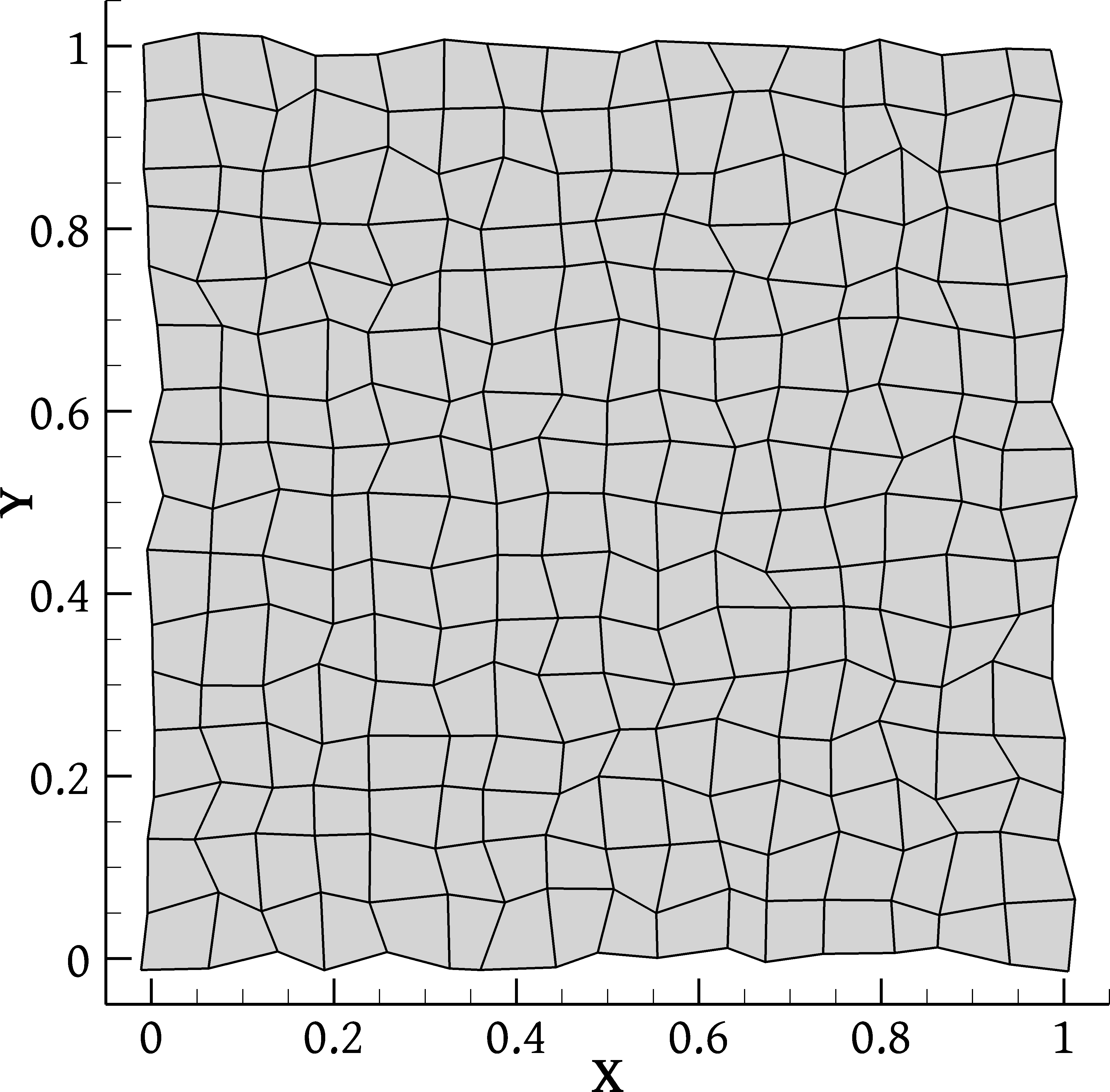
(c) Perturbed grid, $l=3$

Figure 3: Grids of different kinds, at the $l=3$ level of refinement.

1. Structured grids generated by solving a set of elliptic partial differential equations, such as that depicted in Fig. 3(a) (see [19] for construction details). Such grids exhibit skewness, unevenness and non-orthogonality, but the first two qualities diminish with refinement.

2. Cartesian grids with local refinement patches, such as that depicted in Fig. 3(b). Finer grids are obtained by splitting every cell, including those of the patches, into four smaller cells. Therefore, all finer grids are similarly patched, and grid qualities are not affected by refinement. These grids are characterised by large, localised skewness and unevenness (confined near the patch interfaces) that do not diminish with refinement.

3. Grids derived from Cartesian ones by random perturbation of their nodes, such as that of Fig. 3(c) – see [19] for details. Skewness, unevenness and non-orthogonality remain large throughout the grid irrespective of refinement.

For each kind of grid we employ 8 levels of refinement, $l=1,2,\ldots 8$, with each successive grid having 4 times as many cells as the previous one; the grids of level $l=3$ are shown in Fig. 3. The tests concern the calculation of the gradient of the function $\phi(x,y)=\tanh(x)\cdot\tanh(y)$. The effect of grid refinement on the mean and maximum errors $\|\tilde{\nabla}\phi(\underline{P})-\nabla\phi(\underline{P})\|$ across all grid cells, where $\tilde{\nabla}\phi$ is the approximate gradient and $\nabla\phi$ is the exact gradient, are plotted in Figs. 4, 7 and 10. In order to not clutter the diagrams, the errors of only a subset of the schemes are plotted. Following [19], for grids (a) and (c) the average error is calculated simply by dividing the total sum by the number of grid cells, whereas for grids (b) the error of each cell is weighed by the cell volume to account for the patches of different fineness. The slopes of the lines in these figures reveal the order of accuracy of the gradients. Additionally, the errors on the finest grid levels ($l=8$) as a function of the inverse-distance weighting exponent $q$ are plotted in Figs. 5, 6, 8, 9, 11 and 12 (the gradients LSX and LSDX included in these figures will be defined and discussed in Sec. 7.3). At this level of fineness all methods have reached their asymptotic rate of convergence.

On the smooth structured grids, refinement causes the mean errors (Fig. 4(a)) to decrease at a second-order rate, despite the gradients being nominally only first-order accurate (Eq. (5)). This is due to the property that structured grids generated by the solution of differential equations possess, that their skewness and unevenness diminish through refinement (see [19] for an explanation). This causes truncation error component cancellations of the sort described in Sec. 6.2, increasing the order of the leading-order truncation error term. The same happens even with the (nominally inconsistent) common Green-Gauss (GG) gradient which is included for comparison purposes in Fig. 4. However, the performance of the GG gradient is amongst the poorest. The unweighted LS gradient also performs poorly, while the gradients’ performance improves with increase of the weighting exponent $q$ up to $q=2$ for the TG gradients and $q=3$ for the LS gradients (Fig. 5). For larger $q$ the performance deteriorates. The most accurate gradient in this case appears to be the TG(2). This gradient, together with LS(3), LSA(3) and LSD(3), benefit from the even more special situation described in Sec. 6.2, namely they retain their second-order accuracy even at boundary cells, as verified by Fig. 4(b); it is at these cells that the maximum errors occur for the other gradients, seen to decrease at only a first-order rate in Fig. 4(b). Despite this advantageous property, the performance of the LSA gradient is comparatively poor – see also Figs. 5, 6. It is worth noting that the TGI(0) gradient (the QG gradient) performs quite well, much better than its inconsistent GG counterpart, and even significantly better than the un-interpolated TG(0) gradient.

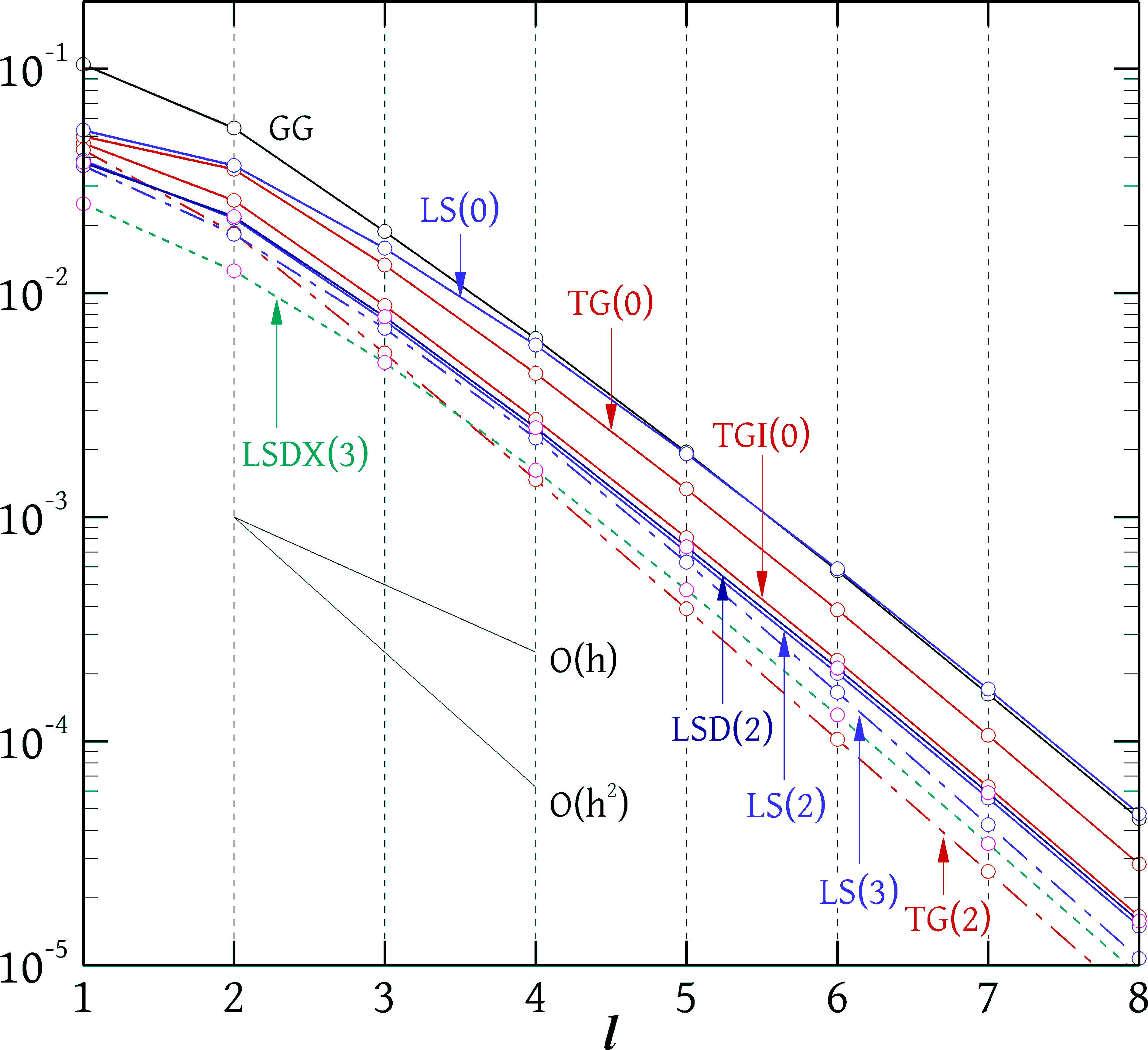
(a) Mean errors

(b) Maximum errors

Figure 4: Minimum and maximum errors of gradient schemes versus refinement level $l$, for the elliptic grids (Fig. 3(a)).

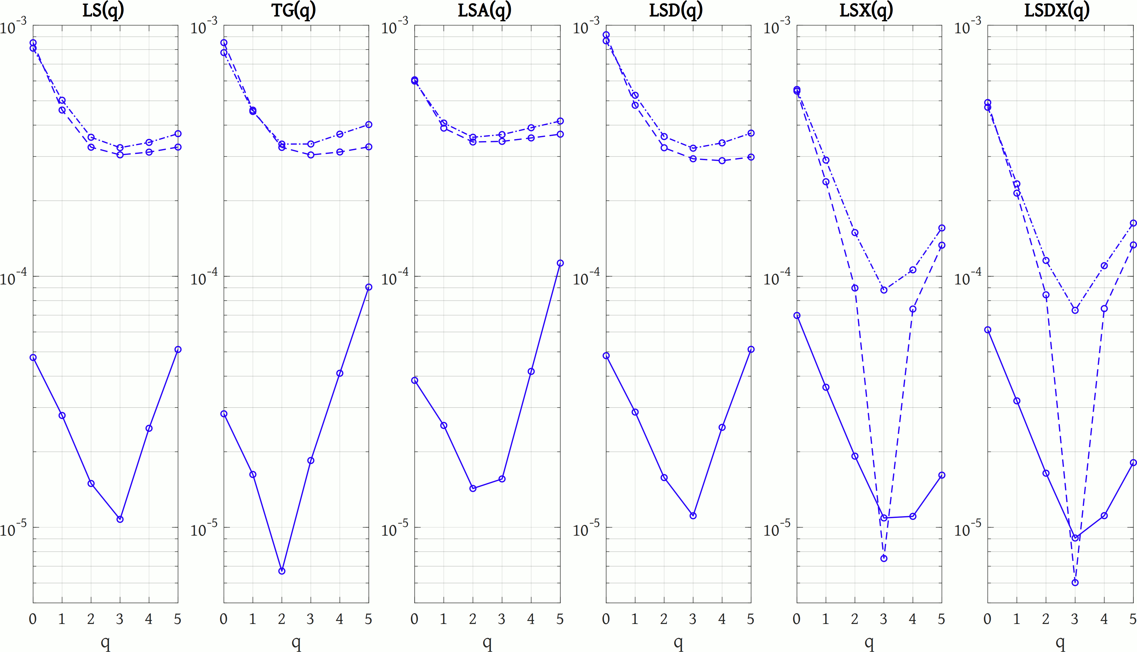
Figure 5: Average errors of various gradient schemes as a function of the exponent $q$, on the finest ($l=8$) elliptic grids. Continuous lines: original structured grid (Fig. 3(a)). Dashed lines: orderly triangulated grid (Fig. 13(a)). Dash-dot lines: randomly triangulated grids (Fig. 13(b)).

Figure 6: Maximum errors of various gradient schemes as a function of the exponent $q$, on the finest ($l=8$) elliptic grids. Continuous lines: original structured grid (Fig. 3(a)). Dashed lines: orderly triangulated grid (Fig. 13(a)). Dash-dot lines: randomly triangulated grids (Fig. 13(b)).

The locally refined grids (Fig. 3(b)) are essentially uniform Cartesian over most of the domain, except near the patch interfaces. Such grids could, for example, be used in flow simulations in combination with immersed boundary methods. On Cartesian grids, all gradient schemes reduce to the same (second-order accurate) simple formula. Hence the differences between the mean errors plotted in Fig. 7(a) are due solely to cells at patch interfaces (details on the topology of these cells, which induces skewness and unevenness, can be found in [19]) and boundaries. Since these cells are a small minority, the mean errors of the various gradient schemes do not differ by much. As can be seen in Fig. 7(a), the mean error of all gradient schemes that fall into the presently proposed general framework decreases at a second-order rate. However, at the cells near the patch interfaces, where there are large skewness and unevenness, the gradients are only first-order accurate, yet the number of these cells is too small to have a effect on the rate of convergence of the mean error (see [19] for a more quantitative discussion). The mean errors of the LS(3), LSA(3), LSD(3) and TG(2) gradients are affected favourably by the second-order accuracy that these schemes enjoy at boundary cells, but in this particular experiment we are mostly interested in what happens at the patch interfaces. The maximum errors, plotted in Fig. 7(b), are more helpful in this respect. They all decrease at a first-order rate (including for the LS(3), LSA(3), LSD(3) and TG(2) gradients, which means that they do not occur at boundary cells but at patch interface cells). Additionally, again Figs. 8 and 9 show the variation of the mean and maximum errors on the finest grid with respect to the inverse-distance weighting exponent $q$. From these results, we can see that inverse distance weighting can help substantially, up to $q=3-4$. Furthermore, the fact that coarse cells at patch interfaces have two neighbours on the fine patch side creates a directional clustering situation, and the accuracy suffers in the absence of any mitigative measures. LSA, LSD and TG gradients do incorporate mitigation strategies (area or directional weighting), unlike LS gradients whose accuracy obviously suffers. Interestingly, the TGI(0) (QG) gradient again performs decently, better than TG(0) or TG(1). In fact, Figs. 8 and 9 show that within the TGI($q$) family, inverse distance weighting is not beneficial, and the best performance is obtained for $q=0$.

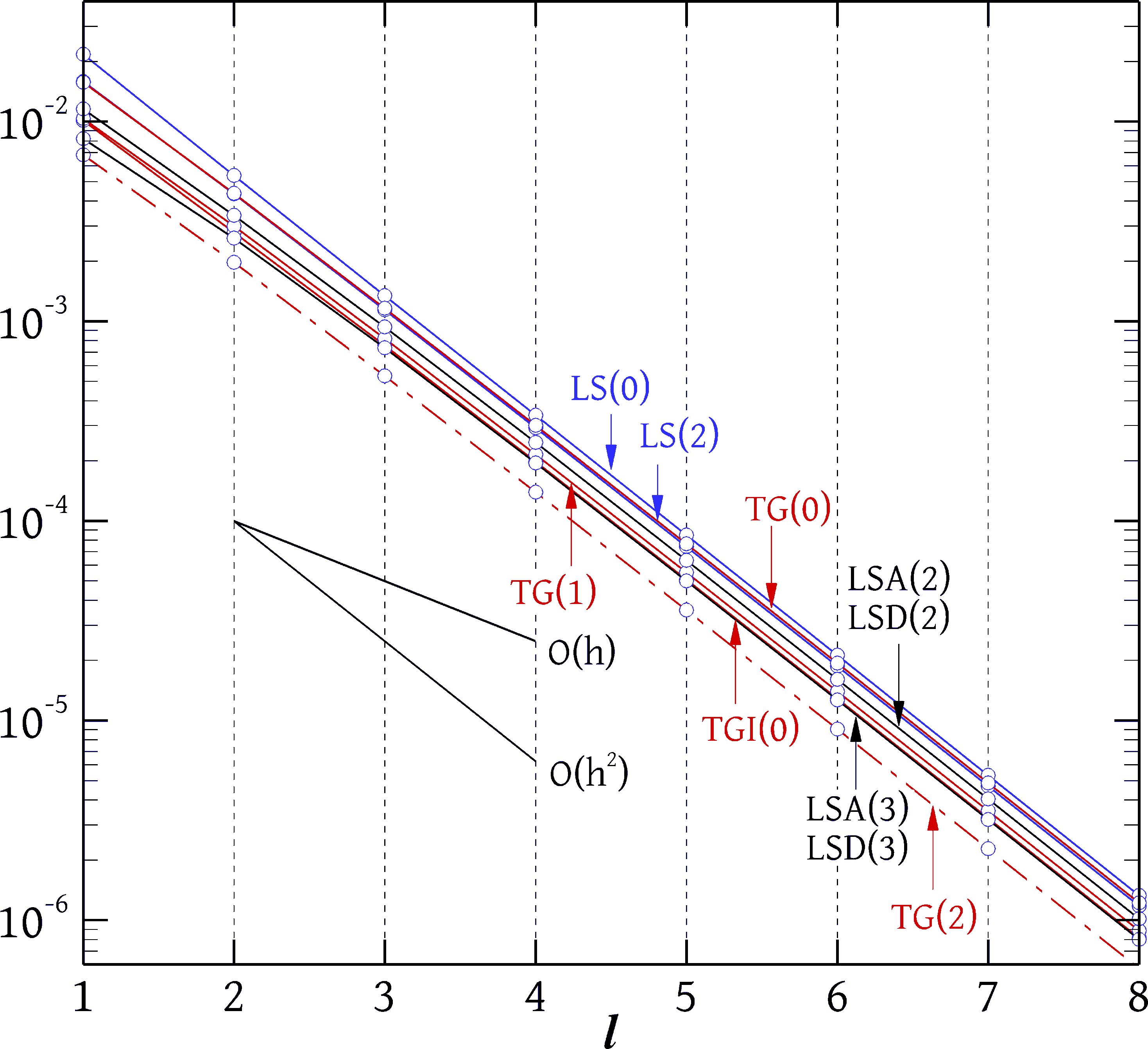
(a) Mean errors

(b) Maximum errors

Figure 7: Minimum and maximum errors of various gradients versus refinement level $l$, for the locally refined grids (Fig. 3(b)).

Figure 8: Average errors of various gradient schemes as a function of the exponent $q$, on the finest ($l=8$) locally refined grid.

Figure 9: Maximum errors of various gradient schemes as a function of the exponent $q$, on the finest ($l=8$) locally refined grid.

Moving on to the randomly perturbed grids, Fig. 10 shows that all methods are first-order accurate with respect to the mean error as well as the maximum error. This behaviour is expected, as these grids exhibit arbitrary, non-diminishing skewness and unevenness throughout the domain and there are no special conditions that could increase the order of accuracy beyond the nominal first-order of Eq. (5) through error cancellations. Figures 10, 11 and 12 show that the best and worst performers are the LS(0) and LSD(3) gradients, respectively, but the differences are quite small and no gradient has a decisive advantage. Again, inverse distance weighting helps up to $q=2-3$, but only slightly in the present case.

(a) Mean errors

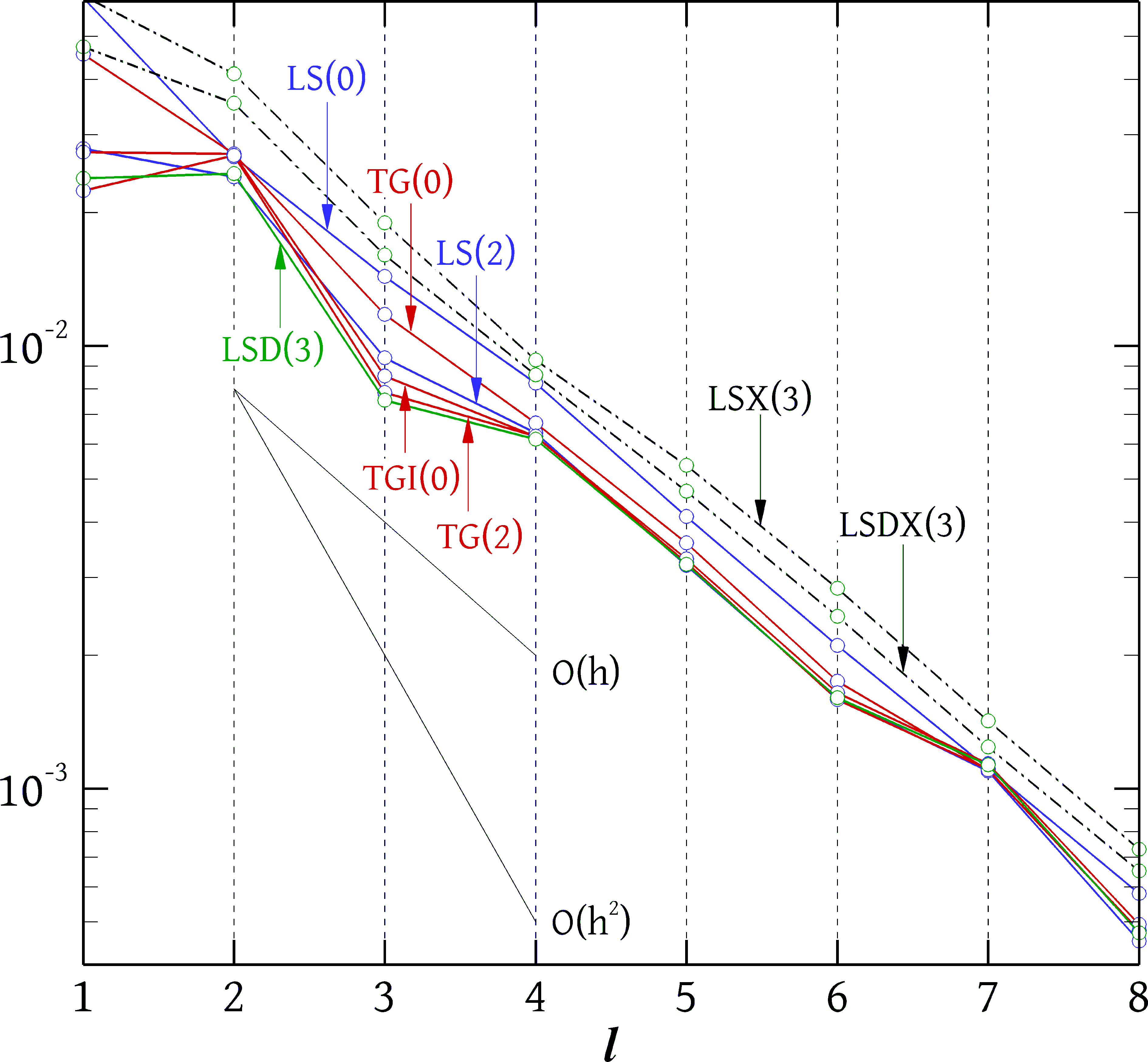
(b) Maximum errors

Figure 10: Minimum and maximum errors of various gradients versus refinement level $l$, for the randomly perturbed grids (Fig. 3(c)).

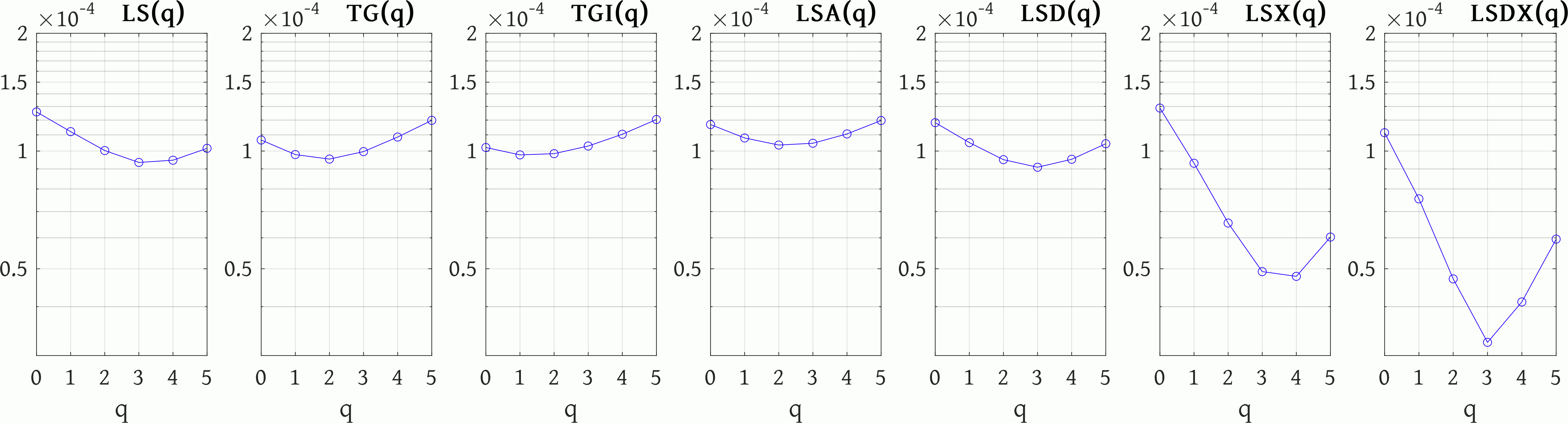
Figure 11: Average errors of various gradient schemes as a function of the exponent $q$, on the finest ($l=8$) randomly perturbed grid.

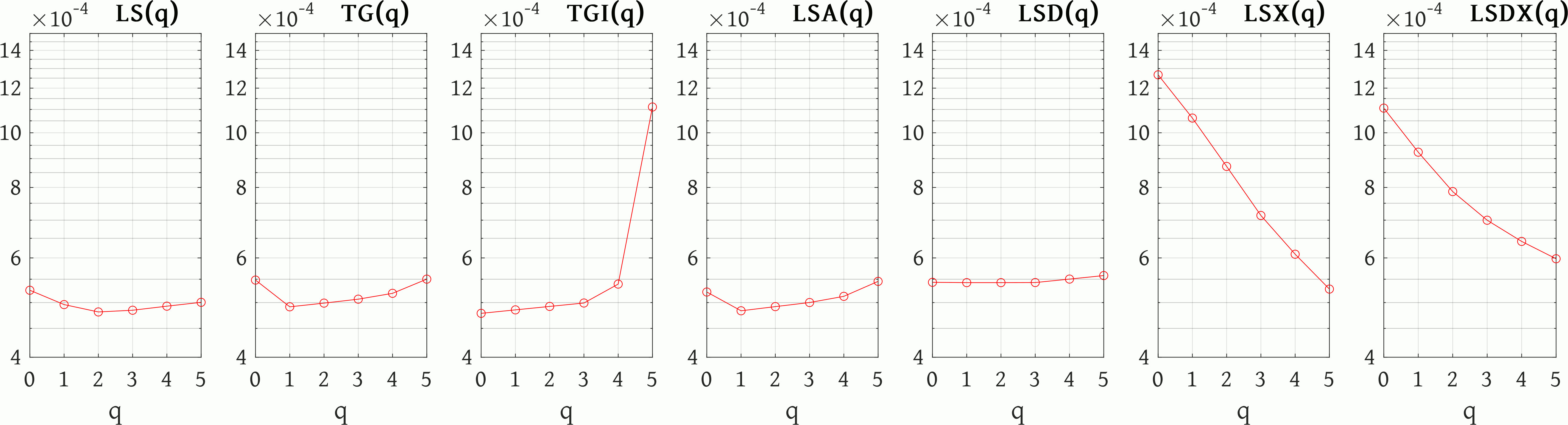
Figure 12: Maximum errors of various gradient schemes as a function of the exponent $q$, on the finest ($l=8$) randomly perturbed grid.

7.2 Grids of triangles

Grids consisting of triangles are quite popular due to the availability of corresponding automated meshing algorithms, which greatly reduce the pre-processing time required for solving a problem. This advantage usually comes at a price of a loss of accuracy compared to structured grids or grids of quadrilaterals in general (similar observations hold also in three-dimensional space). In the present Section, we test the performance of the gradient schemes on triangular meshes. Figure 13 shows the three kinds of meshes used: the first two are based on the elliptically generated structured meshes of Sec. 7.1 (Fig. 3(a)) which have been triangulated by splitting each quadrilateral into two triangles, either along the same diagonal, as in Fig. 13(a), or along a random diagonal, as in Fig. 13(b). The third group of meshes were constructed using the Gmsh mesh generator [35], v. 4.8.4, which was used to tessellate a quarter-disc-shaped domain, of unit radius, as in Fig. 13(c).

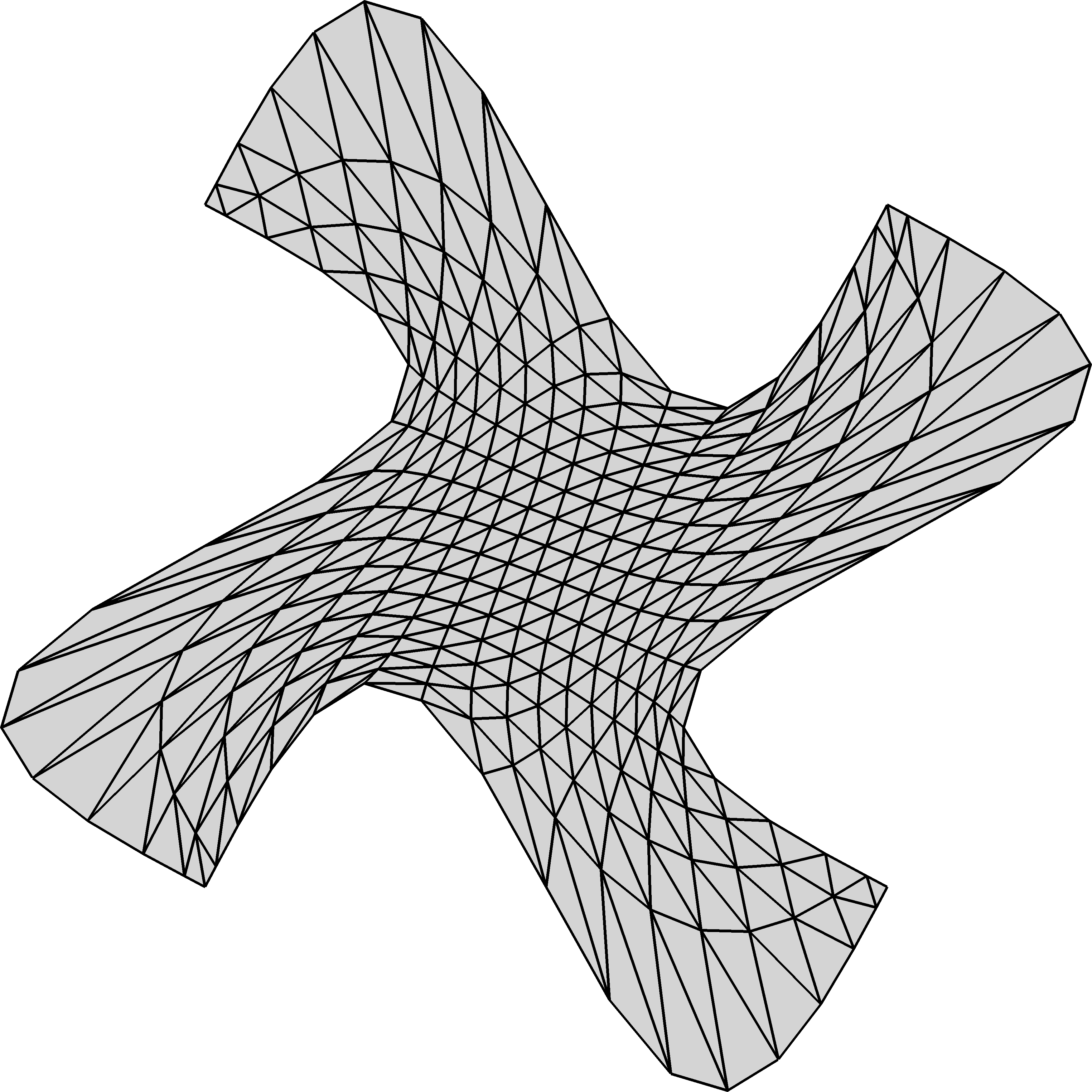
(a) Orderly triangulated elliptic grid

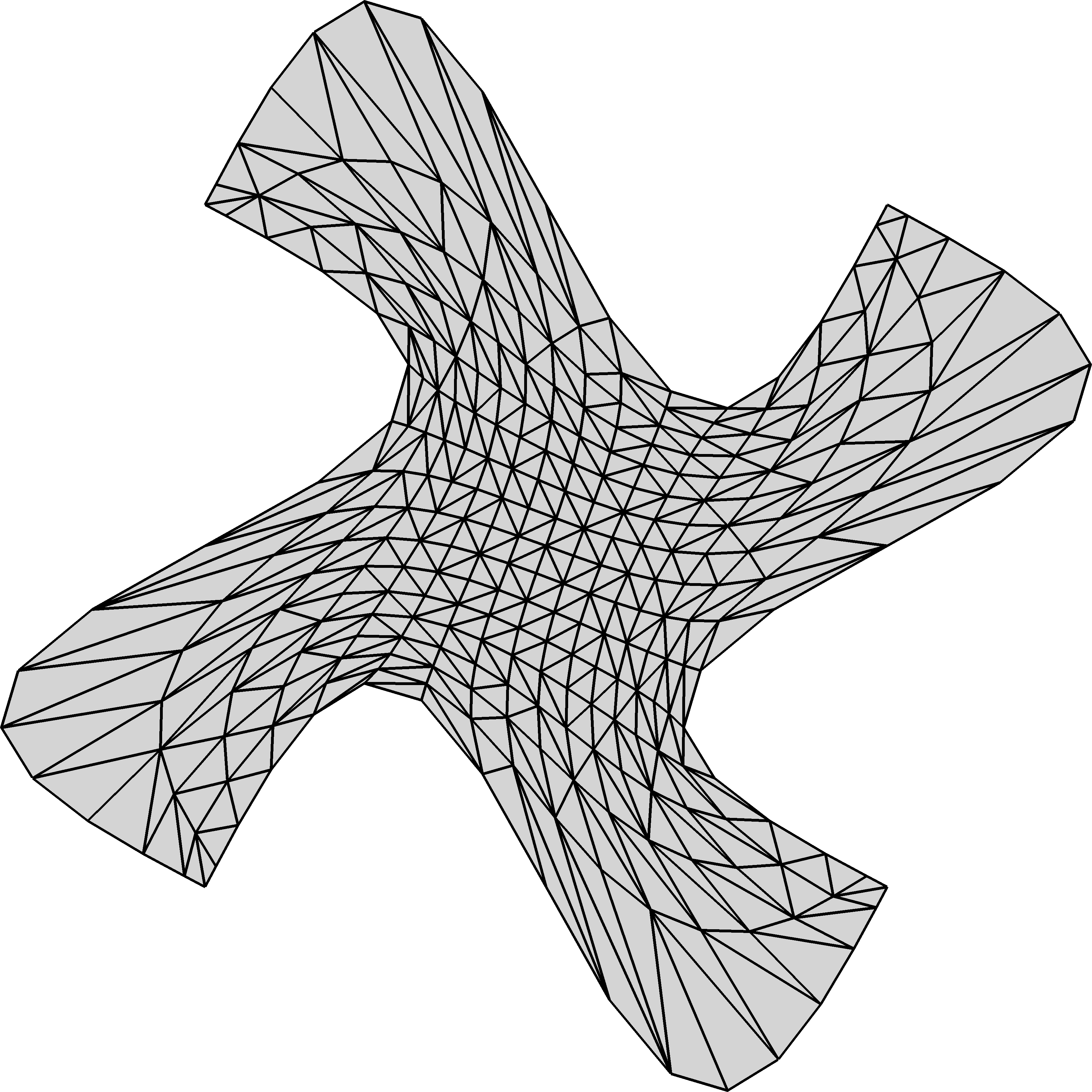
(b) Randomly triangulated elliptic grid

(c) Gmsh grid

Figure 13: Grids of triangles, at the $l=3$ level of refinement.

Mean and maximum errors on the triangulated elliptic grids are plotted in Fig. 14; some errors on the original (quadrilateral) elliptic grids are also included for comparison. In order not to clutter the plots, only the errors of a small subset of the gradients are plotted. The errors of all the gradients on the finest grids ($l=8$) are plotted in Figs. 5 and 6, together with the errors on the original, quadrilateral, structured grids. Excluding for the moment the LSX and LSDX gradients, which will be defined and discussed in Sec. 7.3, we see in Fig. 5 that the mean errors of the LS, LSA, LSD and TG gradients are very similar, and depend mostly on the exponent $q$ than on the gradient scheme. Hence in Fig. 14(a) only the TG(0) and LS(2) errors are plotted, which lie near the higher and lower ends of the spectrum, respectively. The LSA gradient appears to perform worst. The accuracy is usually better on the uniformly triangulated grids (Fig. 13(a)) than on the randomly triangulated (Fig. 13(b)), which is not surprising. The error difference between these two kinds of grids is larger when it comes to the maximum error – Fig. 6.

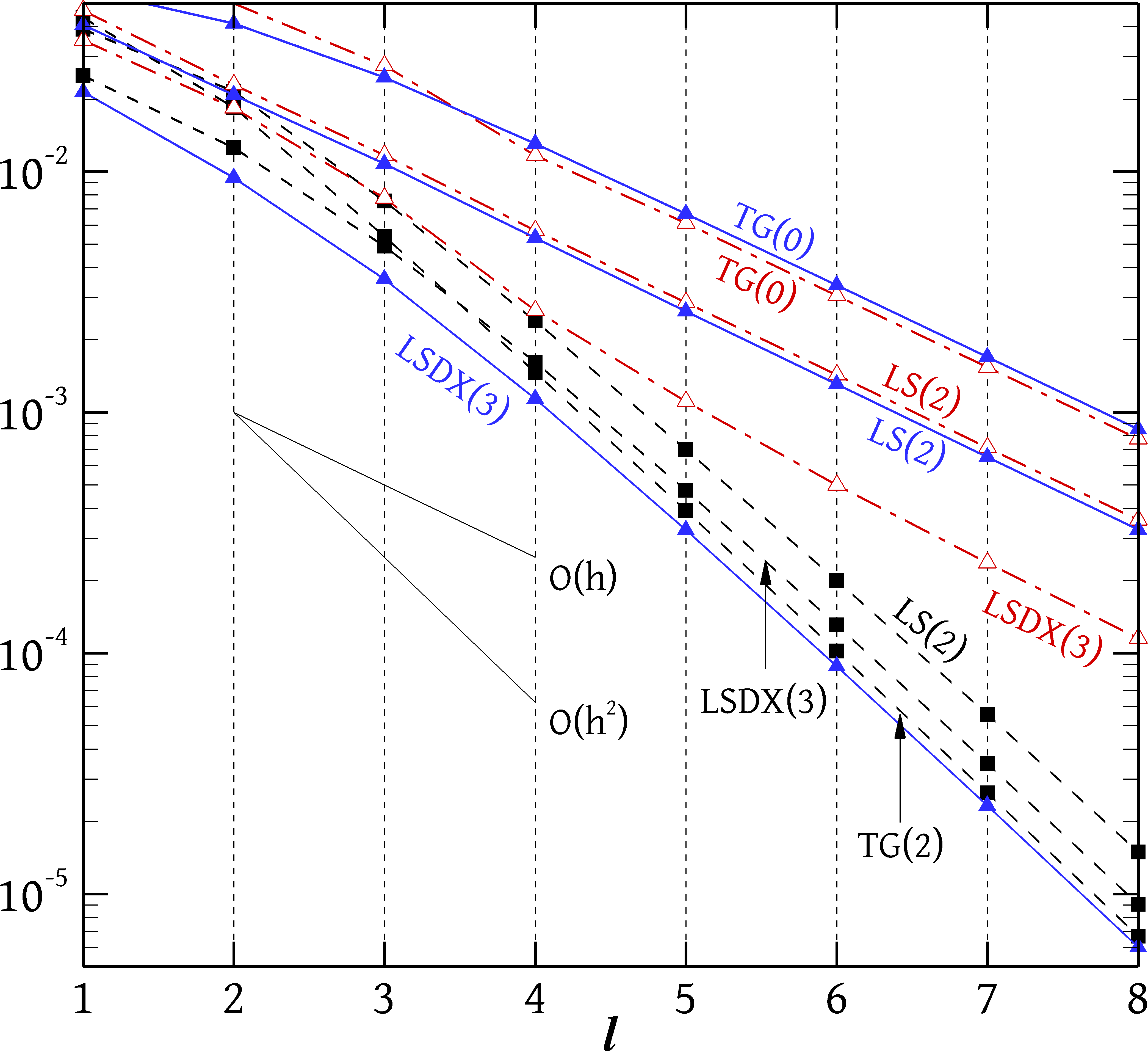
(a) Mean errors

(b) Maximum errors

Figure 14: Minimum and maximum errors of gradient schemes versus refinement level $l$, for the triangulated elliptic grids (Fig. 3(a)). Continuous blue lines ($\blacktriangle$): uniformly triangulated grids (Fig. 13(a)). Dash-dot red lines ($\vartriangle$): randomly triangulated grids (Fig. 13(b)). Dashed black lines ($\blacksquare$): original structured (quadrilateral) grids (Fig. 3(a)).

Concerning the order of accuracy, the LS, LSA, LSD and TG gradients are first-order accurate on both kinds of triangulated structured grid, with respect to both the mean and maximum errors (Fig. 14). This contrasts with the original, quadrilateral structured grid, where all these gradients are second-order accurate with respect to the mean error, while the LS(3), LSA(3), LSD(3) and TG(2) are also second-order accurate with respect to the maximum error, as discussed previously. This is due to error cancellations between opposite faces, as discussed in Sec. 6.2, but in the case of triangulated grids there are no opposite faces and such cancellations do not occur, hence the accuracy remains of first order. Consequently, the gradients can produce 1-2 orders of magnitude larger errors on the finest triangulated grids than on the finest quadrilateral grid, despite the former having twice as many cells.

In fact, a more meticulous examination of the slopes of the maximum error lines in Fig. 14(b) shows that the situation is slightly worse, with the order of convergence being below one, at about $0.6-0.9$ in most cases. This is another instance where the effect of refinement on the grid quality influences the observed order of convergence. The LS, LSA, LSD and TG gradients are formally first-order accurate, provided that grid refinement does not change the quality of the grid. If, however, the refinement procedure is such that the grid quality improves (e.g. opposite faces of quadrilaterals become more aligned, leading to larger error cancellations) or deteriorates then the observed order of convergence may be higher or lower than the formal one.

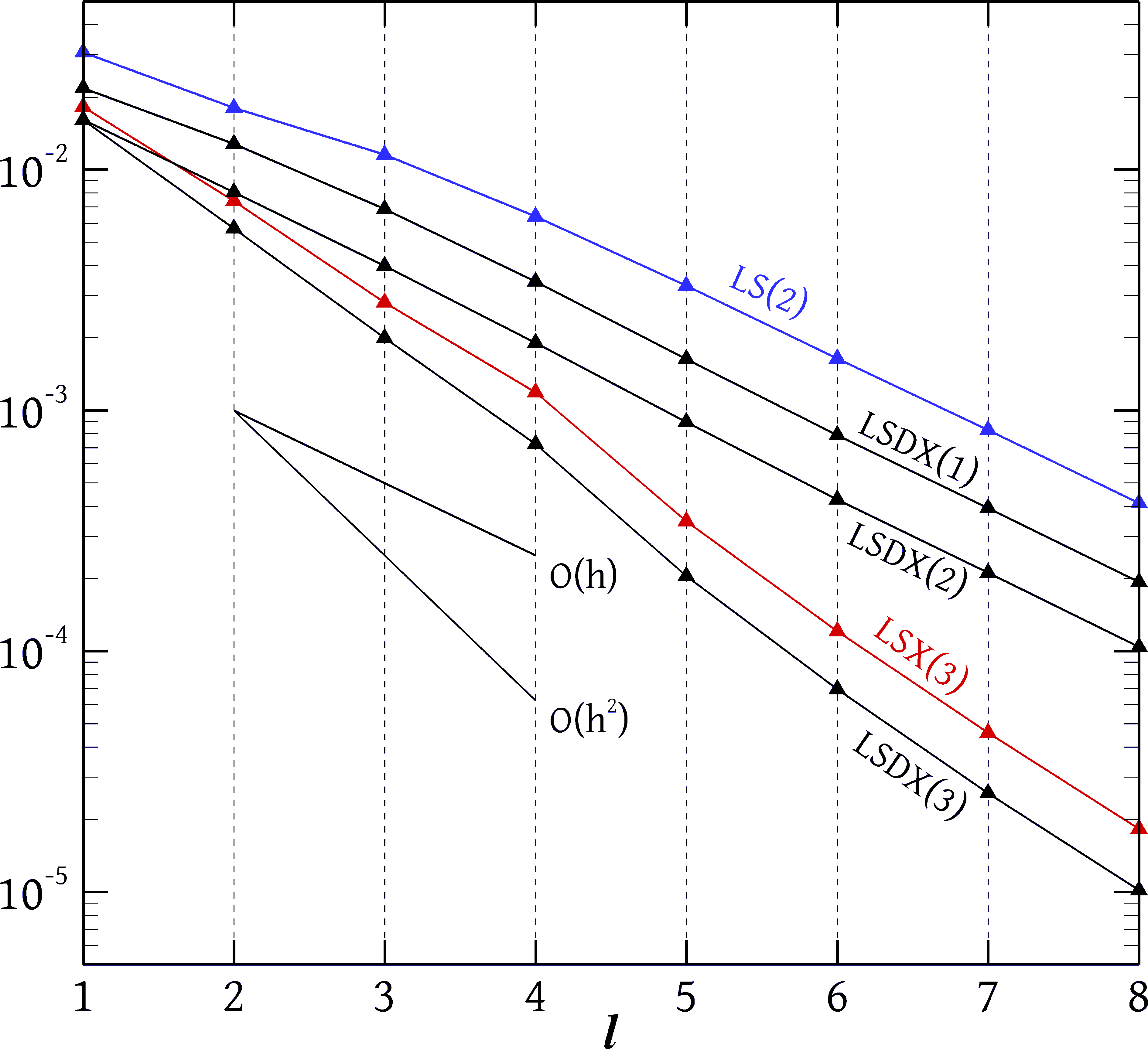
(a) Mean errors

(b) Maximum errors

Figure 15: Minimum and maximum errors of gradient schemes versus refinement level $l$, for the Gmsh grids (Fig. 13(c)).

Next, we consider a series of meshes constructed using the Gmsh mesh generator [35]. The domain is the quarter-disc shown in Fig. 13(c), centred at point (1,1) with additional corners at $(0,1)$ and $(1,0)$. The mesh spacing at each of these three points is set to $2^{-(l+1)}$, where $l$ is the grid level (again, we use 8 grids, corresponding to $l=1,2,\ldots,8$). Furthermore, we impose a mesh spacing of $2^{-(l-1)}$ at point $(0.5,0.5)$, and a mesh spacing of $2^{-(l+3)}$ at point $(0.75,0.75)$. This creates a 16-fold size (length) difference between cells close to $(0.5,0.5)$ and cells close to $(0.75,0.75)$. The $l=3$ grid is shown in Fig. 13(c). It was observed that on these Gmsh meshes the errors of the LS($q$), LSA($q$), LSD($q$) and TG($q$) gradients are nearly identical, for any value of $q$ (see Figs. 16 and 17), and hence we only plotted LS(2) in Fig. (15). The methods are first-order accurate (again, the maximum errors fall at a rate that is slightly below first-order).

Figure 16: Average errors of various gradient schemes as a function of the exponent $q$, on the finest ($l=8$) Gmsh grid.

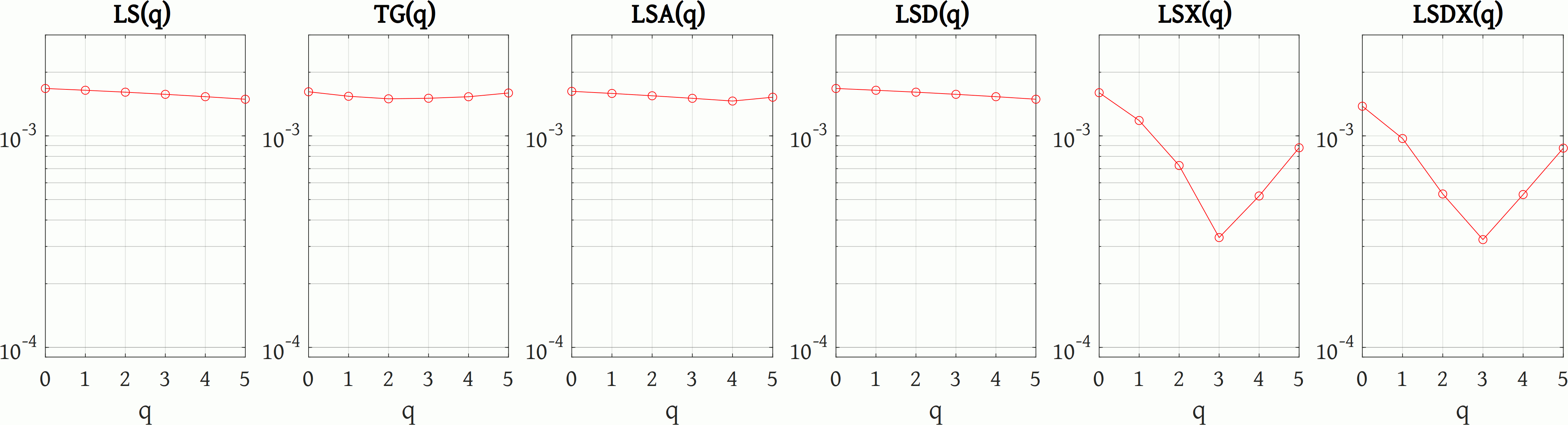
Figure 17: Maximum errors of various gradient schemes as a function of the exponent $q$, on the finest ($l=8$) Gmsh grid.

7.3 Compact vs. extended stencils

In the previous results, the gradients (LS, LSA, LSD, TG, TGI) at the centroid of a cell were calculated using information only from the nearest neighbours of that cell (the cells that share a face with it). These cells are marked as “N” in Fig. 18. Some studies have found it beneficial to include more than just the nearest neighbours in the calculation of the gradient, e.g. [30, 20, 23, 36]. Therefore, we also performed such calculations. In particular, we employed extended stencils that include additionally all other cells (marked as “D” in Fig. 18) that share a vertex with the cell where the gradient is calculated. Unfortunately, not all gradients examined here can employ extended stencils; those whose weight vectors involve geometrical features of the cell’s faces, i.e. LSA, TG and TGI, can only use compact stencils. On the other hand, the LS and LSD gradients are face-free and do not have any restrictions on which neighbours to use. Hence, we applied them also in combination with the extended stencils of Fig. 18, and for convenience we will refer to the resulting schemes as LSX($q$) and LSDX($q$), respectively (LS($q$) and LSD($q$) refer to the use of nearest-neighbour stencils).

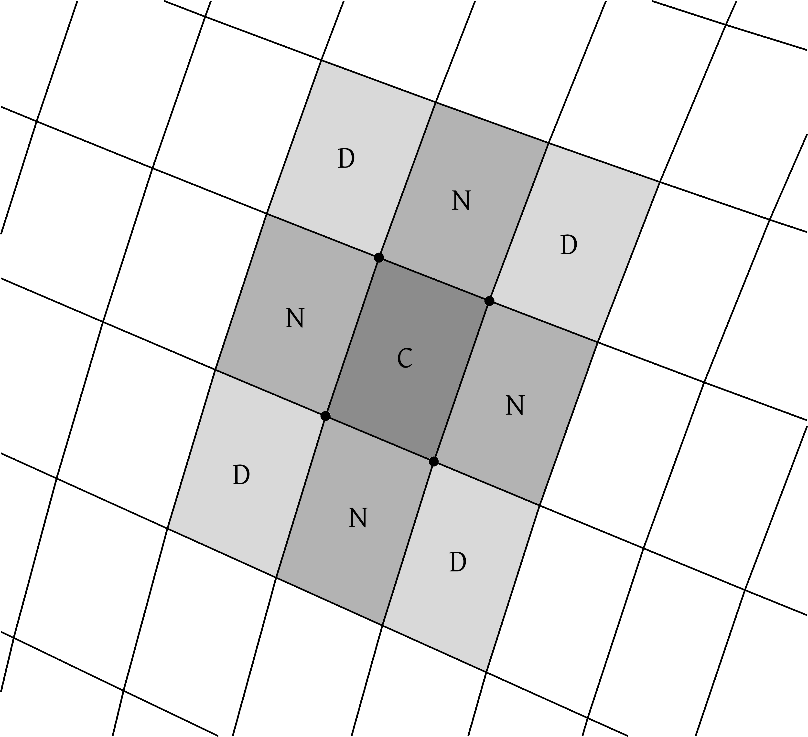
(a) Quadrilateral mesh

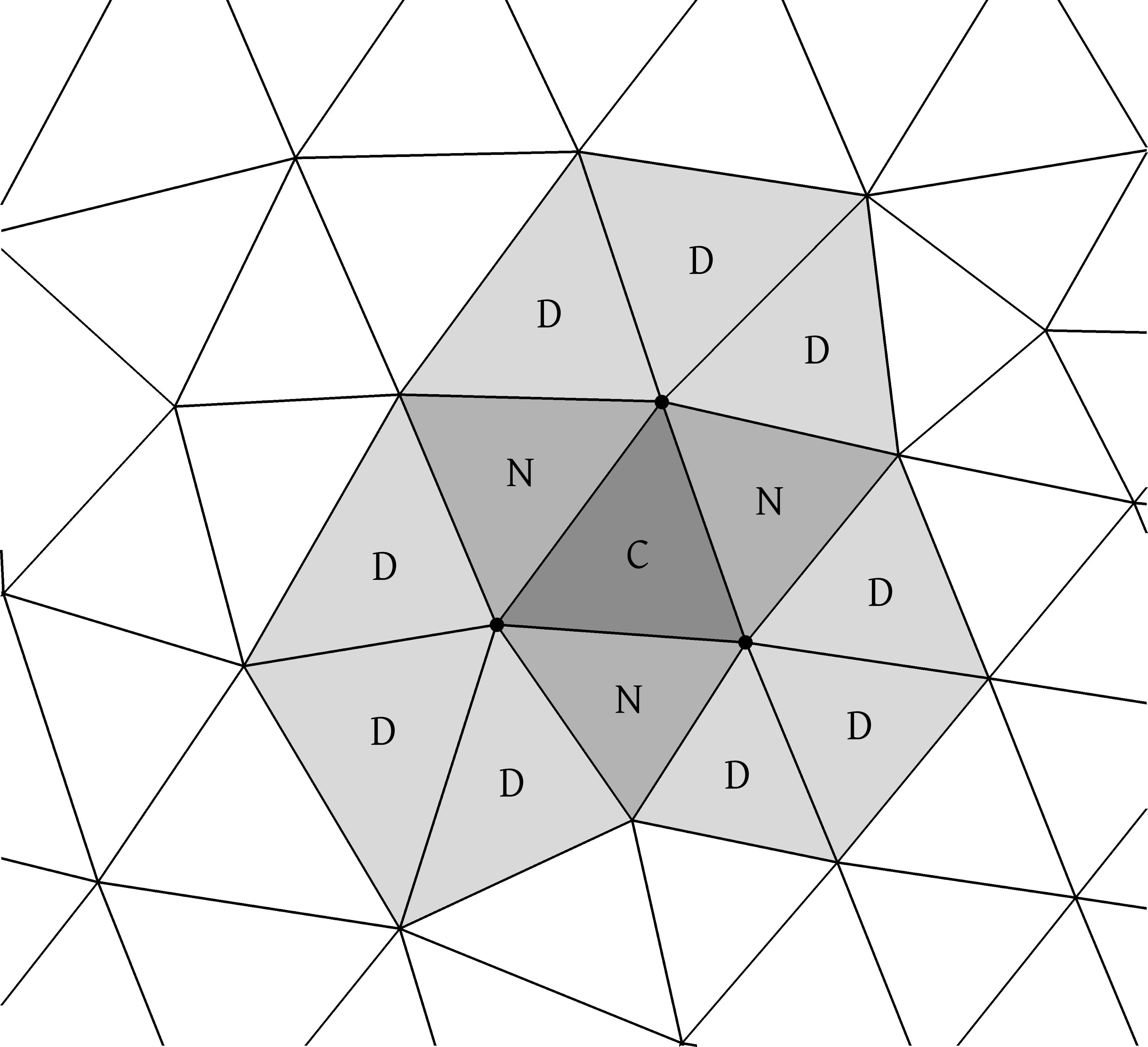
(b) Triangular mesh

Figure 18: Compact and extended stencils for the calculation of the gradients, on quadrilateral 18(a) and triangular 18(b) grids. The gradient is calculated at the centroid of cell ’C’, while ’N’ marks its nearest neighbours (those that share a face with ’C’) and ’D’ its distant neighbours (those that share a single vertex with ’C’).

Results for the LSX and LSDX gradients were also included in the Figures presented thus far. First, let us examine their performance on the elliptic quadrilateral grids (Fig. 3(a)). There, Figs. 4, 5 and 6 show that these gradients perform well; nevertheless, they are outperformed by the TG(2) gradient. Also, Figs. 5 and 6 (quadrilateral grids) show that the optimal range of $q$ for LSX and LSDX is shifted to higher values compared to the compact-stencil gradients. This is not surprising, since the additional neighbours that LSX and LSDX involve will usually lie at greater distances than the nearest neighbours, and hence contribute larger distance-related truncation errors, which are minimised by increasing the distance-weighting exponent $q$. On the other hand, these additional neighbours contribute information from more directions, which may be beneficial for accuracy, provided that $q$ is large enough, so that, for example, for $q>3$, LSX and LSDX are much more accurate than LS, LSA, LSD or TG. It is also noteworthy that the maximum errors of the LSX and LSDX gradients on the quadrilateral grids are, in general, larger than those of the nearest-neighbour gradients (Fig. 6), which can also be attributed to large distances of additional neighbours. Finally, we can note that, as seen in Figs. 4 and 14, the extended-stencil gradients outperform the compact stencil gradients on coarse structured grids, where skewness and unevenness are still large and the benefits of structured refinement, which grant 2nd-order accuracy (Sec. 6.2), have not yet manifested.

So, the extra data structures and computational cost associated with the extended stencils is rather unwarranted in the quadrilateral elliptic grids’ case. However, the situation changes dramatically when these grids are triangulated. Figure 5 shows that extending the stencil can reduce the error by a factor of 50 on the finest orderly triangulated grid, and by a factor of 4.5 on the finest randomly triangulated grid. The LSDX gradient is slightly more accurate than the LSX. It is striking in Fig. 5 that the LSDX(3) error on the orderly triangulated grid is smaller than any other error, including that on the quadrilateral grids. Figure 14(a) shows that the LSDX(3) gradient is nearly 2nd-order accurate on the orderly triangulated grids (so is the LSX(3) gradient, not shown). This is because, on the orderly triangulated grid, the cells of the extended stencil tend to align pairwise, giving rise to the situation described in Sec. 6.2 where the $q=3$ exponent causes error cancellations between opposite neighbours. On the randomly triangulated grids no such perfect alignment occurs, but nevertheless the multitude of directions associated with the many neighbours gives opportunities for partial cancellations of errors, so that the LSX(3) and LSDX(3) gradients are still substantially more accurate than the rest.

A similar large benefit is brought about by extending the stencil on the Gmsh grids, as Figs. 16 and 17 show. The Gmsh algorithm appears to generate grids that are similar to the orderly triangulated elliptic grid over parts of the domain (Fig. 13(c)). The extended stencils give rise to error cancellations that increase the order of accuracy of the LSX(3) and LSDX(3) gradients to about 1.5, as the slopes of the corresponding curves of Fig. 15(a) reveal. Directional weighting again brings a modest increase in accuracy (LSDX(3) is more accurate than LSX(3)).

Finally, significant benefits of extending the stencil are also evident in Figs. 10(a) and 11: on the randomly perturbed quadrilateral grids the LSDX(3) and LSX(3) gradients have mean errors that are approximately 3 and 2 times smaller, respectively, than those of the compact stencil gradients. The LSX(3) and LSDX(3) gradients are ultimately first order accurate, although, as Fig. 10(a) shows, on coarser grids they exhibit second-order convergence. When it comes to the maximum error, Figs. 10(b) and 12 show that, on the contrary, the extended stencil gradients exhibit large maximum errors. This can again be attributed to distant cells being included in the stencil in some cases, and is remedied by increasing the exponent $q$ (Fig. 12).

8 Further numerical tests: curved geometry with grids of high aspect ratio

8.1 The tests and their results

A situation that is quite challenging for gradient discretisation schemes and has gathered attention from researchers is that of domains with curved boundaries meshed with cells of very high aspect ratio, as typically used for the simulation of high-speed boundary layer flows in aerodynamics (e.g. [29, 30, 37, 20, 23]). Hence it was included in the current set of experiments. Figure 19 shows part of such a grid (the aspect ratio is reduced for clarity), which shall henceforth be referred to as HARC (High Aspect Ratio Curved) grid. The grid of Fig. 19 is structured and a compact stencil is marked, but we will also examine triangulated grids and extended stencils. The structured grid case is important, because it is a popular strategy to use a structured grid near the boundary, in order to achieve high accuracy, even if farther from the boundary the grid is unstructured.

Oftentimes, the differentiated variable’s contours more or less follow the shape of the boundary. In this case, the curvature introduces a nonlinearity that poses a challenge to gradient schemes like the ones considered here, which are founded on an assumption of linear variation of the variable in the neighbourhood of the cell. Furthermore, due to the large aspect ratio, the magnitudes of the contributions of different faces can differ by several orders of magnitude, depending on the weighting scheme. The unweighted LS gradient is particularly notorious. With reference to Fig. 19, LS(0) places equal emphasis on satisfying $\Delta\phi_{f}=\nabla\phi(\underline{C}_{0})\cdot(\underline{C}_{f}-\underline{C}_{0})$ for $f=1$ (or $3$) as for $f=2$ (or $4$). For $\gamma>1$, where $\gamma$ is the ratio of the $y-$displacement of $\underline{C}_{1}$ to that of $\underline{C}_{4}$, both of them with respect to $\underline{C}_{0}$ (Fig. 19), this results in the LS(0) gradient underestimating the actual $\partial\phi/\partial y$ at $\underline{C}_{0}$ by a factor of approximately $\gamma$. The resulting inaccuracy can be very severe, as in practical applications $\gamma$ can be as high as $50$ or greater [29]. Using proper weighting (inverse distance) greatly improves the accuracy.

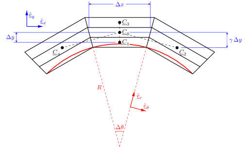
Figure 19: Structured grid of high aspect ratio cells over a curved boundary (the aspect ratio is shown greatly reduced for clarity).

So, we first construct a structured HARC grid over a circular arc of radius $R=1$, like the one shown in Fig. 19. The grid spans from $\theta=-0.256$ to $\theta=+0.256$ radians in the azimuthal direction, with a corresponding spacing of $\Delta\theta_{l}=0.256/2^{l}$ radians, for levels of refinement $l=0,1,\ldots,9$. The radial spacing is $\Delta r_{l}=R\,\Delta\theta_{l}/A$ where $A=1000$ is the cell aspect ratio. Grid level $l=0$ has $2\times 2$ cells, and grid level $l=9$ has $1024\times 1024$ cells in the $(r,\theta)$ directions.

The first function to be differentiated is selected to vary only in the radial direction:

$$\phi(r)\;=\;\tanh\left(f(r)\right)\qquad\text{where}\qquad f(r)\;=\;f_{\min}\;+\;(f_{\max}-f_{\min})\frac{r-r_{\min}}{r_{\max}-r_{\min}}$$ (32)

The function $f$ varies linearly in the radial direction, from $f=f_{\min}=1$ at $r_{\min}=R=1$, to $f=f_{\max}=3$ at $r_{\max}=1.0005$ ($r_{\max}$ is close to the outer radius of the grid, which is $1.000512$). Thus the differentiated function $\phi$ varies from $\tanh(1)$ to $\tanh(3)$ across the radial width of the grid. An average value for the magnitude of $\nabla\phi$ is therefore $G=(\tanh(3)-\tanh(1))/0.0005=466.9$.

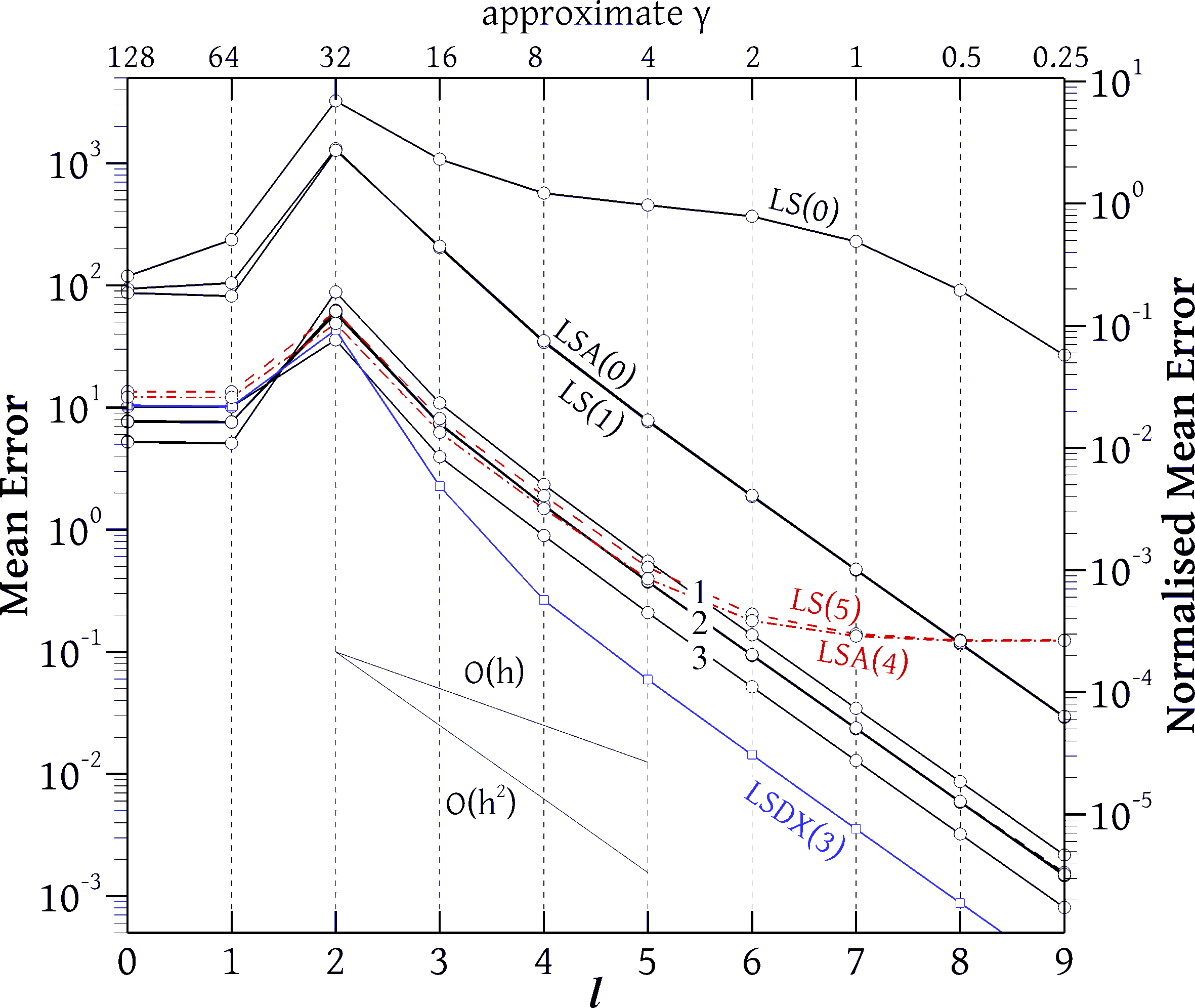
Figure 20: Mean errors of several gradient schemes when differentiating the radial function (32) on the structured HARC grid. Line group 1: TG(0), LSA(1). Line group 2: TGI(0), TGI(1), TG(1), TGI(2), GG, LS(2), LSA(2), LSX(2). Line group 3: TG(2), LS(3), LSA(3), LSDX(4).

Figure 20 shows the mean errors of several gradient schemes, at each refinement level $l$. The left vertical axis shows the mean error, while the right vertical axis shows this error normalised by the average gradient $G$. Many error curves collapse onto the lines labelled “1” (TG(0) and LSA(1)), “2” (TGI(0), TGI(1), TG(1), TGI(2), GG, LS(2), LSA(2), LSX(2)) and “3” (TG(2), LS(3), LSA(3), LSDX(4)). All lines exhibit 2nd-order convergence, which is expected since the grid is structured. The most accurate among these groups is group “3” which includes gradients such as LS(3), LSA(3) and TG(2) that retain 2nd-order accuracy even at boundary cells. Looking at the normalised error, most schemes achieve adequate accuracy except the LS(0) gradient which only gives meaningful results on grids $l\geq 7$, for which $\gamma\leq 1$, in accordance with the theory outlined above. Approximate values of $\gamma$ are printed on the top axis, calculated as $\gamma\approx A\Delta\theta/2$, a valid approximation for small $\Delta\theta$ [29]. On the other extreme, the LSDX(3) gradient stands out as the most accurate by a significant margin. The LSA(0) and LS(1) gradients form a small group of their own; their accuracy is relatively poor, albeit much better than that of the LS(0) gradient. In general, it was observed that the LSA($q$) gradient is almost identical to the LS($q+1$) gradient on this grid, which is not surprising since, for this geometry, weighting by $\|\underline{S}_{f}\|$ is almost equivalent to weighting by $\|\underline{R}\|^{-1}$.

The plot 20 includes the error curves for LS(5) and LSA(4), shown in red dashed and dash-dot lines, respectively. As expected, these curves nearly coincide; however, what stands out is that these errors appear to diverge beyond level $l=5$. This seems to stem from a numeric instability, as repeating the calculations in higher precision arithmetic, 10-byte (extended precision) or 16-byte (quadruple precision), eliminates the divergence and the gradients exhibit second-order convergence down to the finest grid. Depending on the algorithm used to calculate the cell centroids, the instability can be much worse than that shown on Fig. 20. Hence, this issue deserves a deeper investigation, and we devote a separate section to it, Sec. 8.2.

To get a more complete picture, in addition to the structured HARC grid of Fig. 19, other kinds of high-aspect-ratio grids were used as well. This includes a version where the radial grid lines of HARC grids are replaced by oblique ones, at an angle of 45° to the radial direction, as in the sketch of Fig. 21; this family of grids will be referred to as HARCO grids (HARC grids with Oblique grid lines). The other grid families employed are orderly and randomly triangulated versions of the HARC and HARCO grids, in exactly the same fashion that the elliptic grid of Fig. 3(a) gave rise to the triangulated grids of Figs. 13(a) and 13(b).

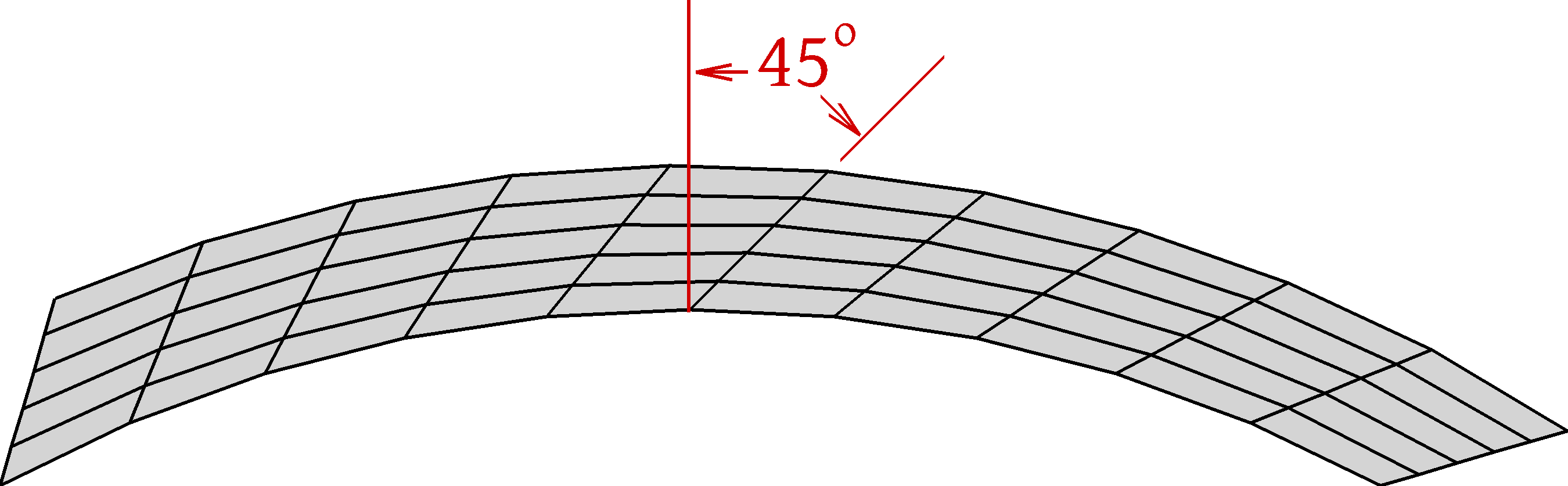
Figure 21: A High Aspect Ratio Curved Oblique (HARCO) grid.

Figure 22 shows the mean normalised (by $G$) errors on the level 6 grids of all these mesh families, as a function of the weighting exponent $q$. The 10-byte calculation results are shown, in order to avoid any pollution by roundoff errors. One can observe the following. The errors on the structured grids are, in general, 1-3 orders of magnitude smaller than on the triangulated grids. The difference is especially huge for the compact-stencil LS and LSD gradients, which perform poorly on the triangulated grids. The difference is smallest for the extended stencil gradients, LSX and LSDX; extending the stencil can increase the accuracy of the LS and LSD gradients on triangulated grids by several orders of magnitude, especially on the orderly triangulated grids. On the quadrilateral grids, the gains from extending the stencil are small, although the best accuracy overall is observed for the LSDX(3) gradient on the HARC quadrilateral grid.

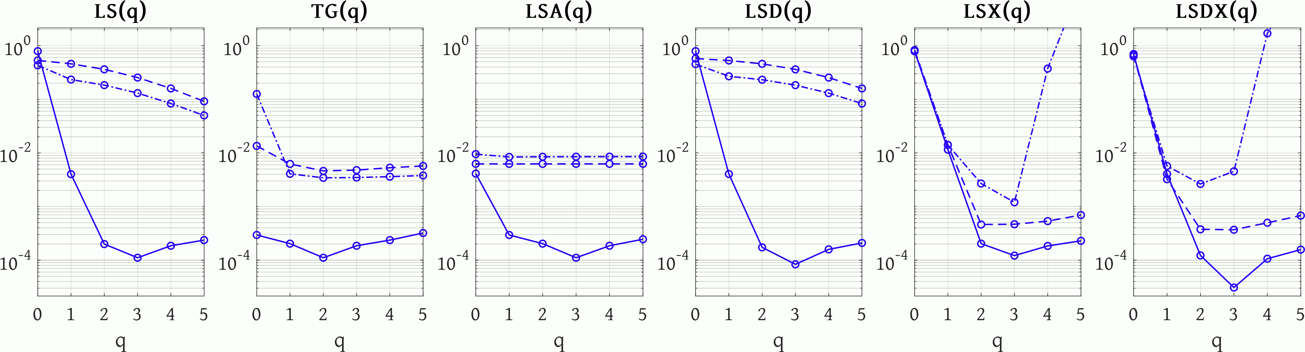
(a) HARC meshes

(b) HARCO meshes

Figure 22: Average normalised errors of several gradient schemes, as a function of the exponent $q$, for computing the gradient of the radially-varying function (32) on the $l=6$ HARC 22(a) and HARCO 22(b) grids. The errors on structured grids are drawn with continuous lines, those on orderly triangulated grids with dashed lines, and those on randomly triangulated grids with dash-dot lines.

The performance of the least-squares gradients is very similar on the HARC and HARCO grids. This is not surprising, given that the least-squares gradients’ geometric input is only or mostly the cell centres, which do not differ much between these two grids. On the other hand, the TG gradient relies heavily also on the face normal vectors, which differ significantly between the HARC and HARCO grids; hence, in the quadrilateral case, Fig. 22 shows that, whereas the TG gradient is quite efficient on the HARC grid, its performance suffers tremendously, to the point of TG becoming unusable, on the HARCO grid if $q>1$. Such impact on the TG gradient performance is not exhibited in the triangulated grids case; one only notices a slight deterioration in the randomly triangulated case.

On triangulated grids, the accuracy is usually better when the triangulation is orderly, but, unlike in the elliptic grid case of Sec. 7 (Figs. 13(a) and 13(b)), the LS and LSD gradients appear to be more accurate on the randomly triangulated grids (as is the TG gradient on the HARC grid). Nevertheless, the accuracies on both kinds of grids are usually comparable. The extended-stencil gradients have a larger advantage on the orderly triangulated grids than on the randomly triangulated ones, as for the elliptic grids of Sec. 7. Surprisingly, on the randomly triangulated grids, the errors of the extended-stencil gradients skyrocket when $q$ is increased beyond 3.

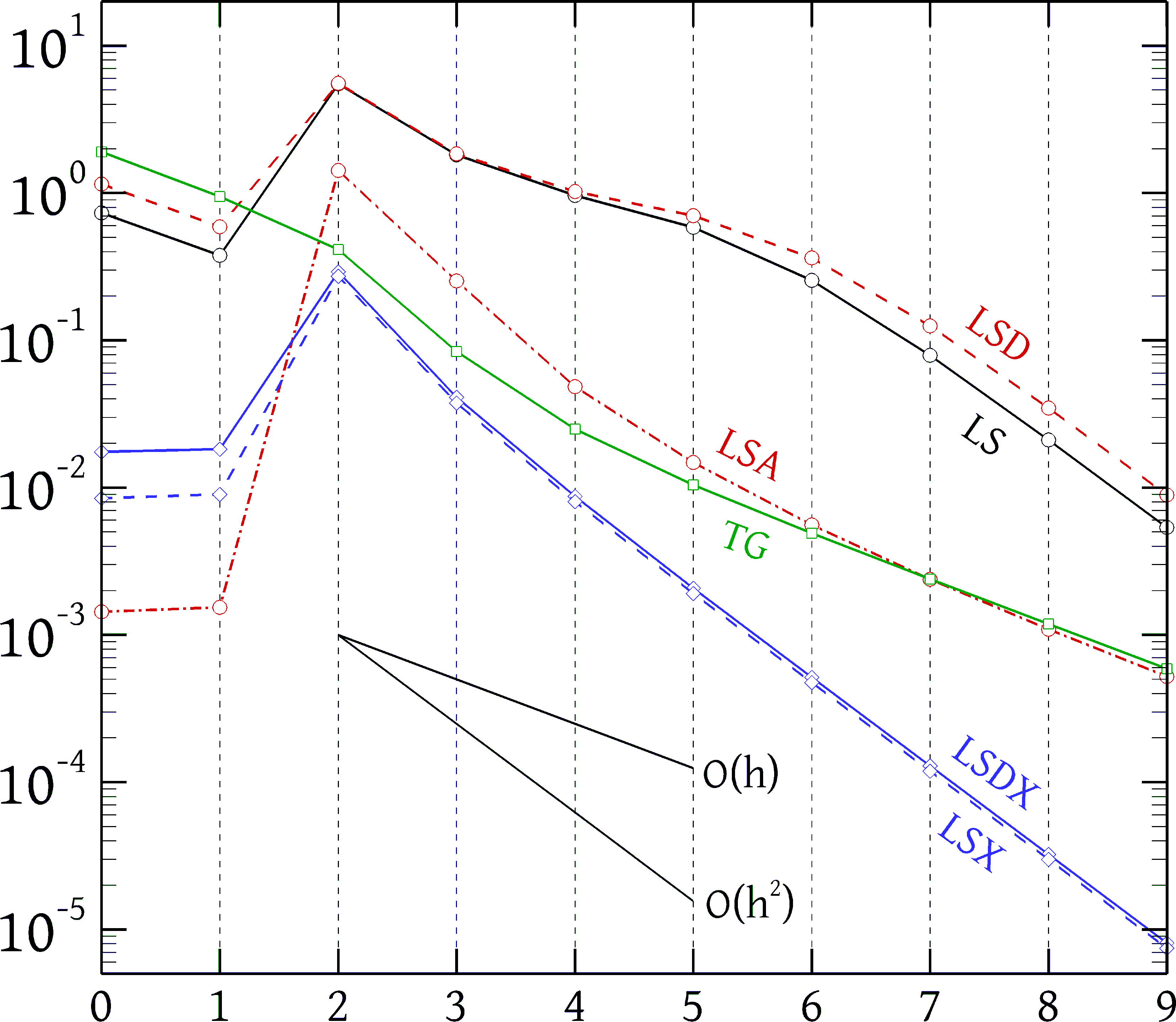
(a) Orderly triangulated HARCO grids

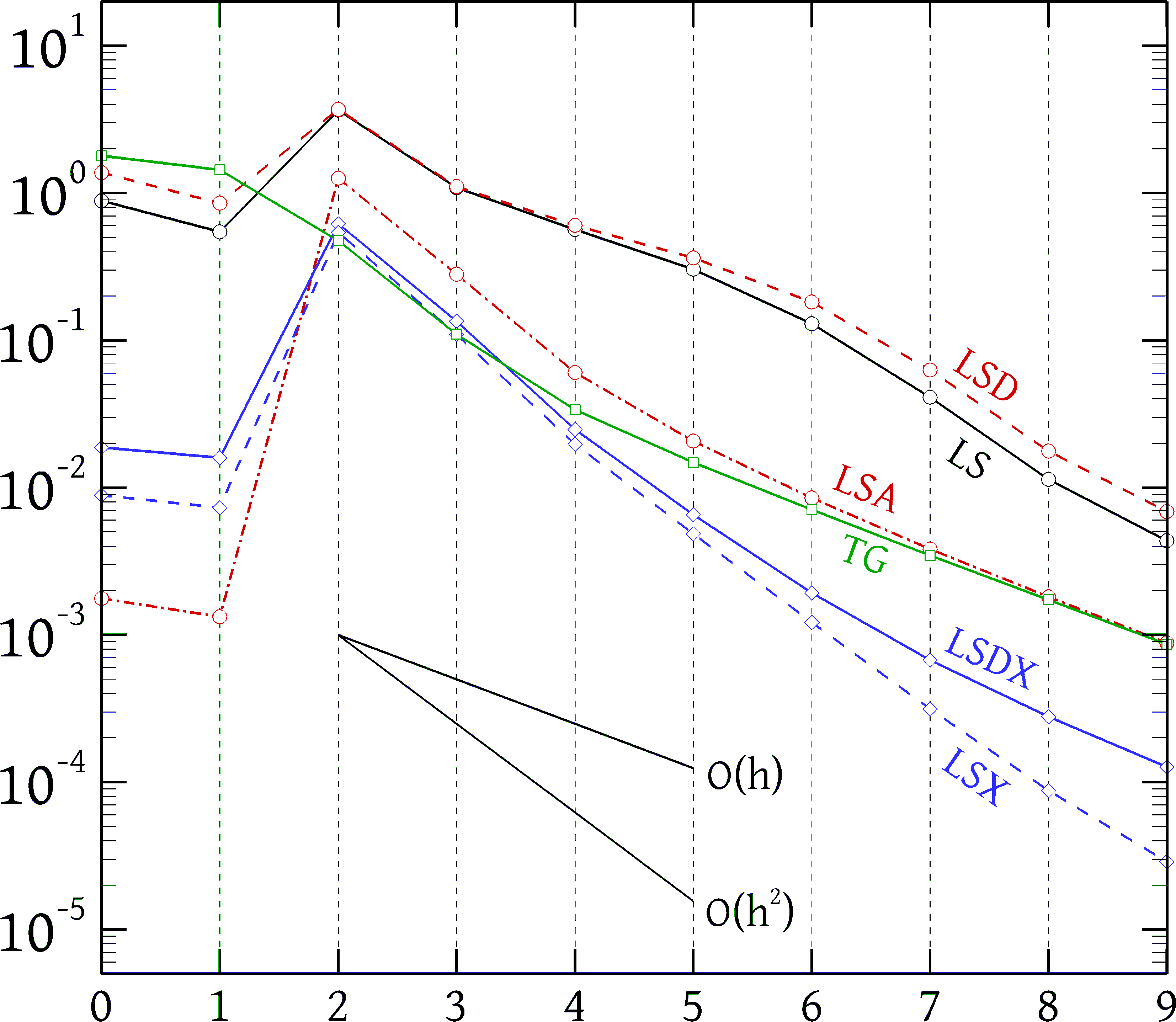
(b) Randomly triangulated HARCO grids

Figure 23: Mean normalised errors of various gradients with $q=3$ weight exponent, on 23(a) orderly triangulated HARCO grids and 23(b), as a function of the grid level. The function differentiated is the radial function (32).

Figure 23 shows the convergence of the mean errors (normalised by $G$) of several gradients, all of which have a weighting exponent of $q=3$, on the triangulated HARCO grids. As noted, the gradients are slightly more accurate on the orderly triangulated grids. On the orderly grids, we can observe the following: compared to the other gradients, the LS(3) and LSD(3) gradients have poor accuracy, but appear to converge at a second-order rate, in contrast with the LSA(3) and TG(3) gradients, which are more accurate but exhibit first-order convergence. Since, on this type of grid, first-order convergence is expected, presumably the convergence of the LS(3) and LSD(3) gradients would downgrade to first-order on even finer levels, as indeed we can see happening on the randomly triangulated grids (Fig. 23(b)). The LSDX(3) and LSX(3) gradients exhibit second-order convergence on the orderly grids, like in the elliptic grid case. On the randomly triangulated grids, the LSX(3) and LSDX(3) convergence rates are of second order on intermediate levels, but taper off towards first-order on the finest levels. Figure 23 (and also Fig. 26(a), to be discussed later) shows that on the HARC and HARCO grids the asymptotic convergence rates may not yet be attained on intermediate levels, and hence a comparison of the gradients on the same grid level, as in Fig. 22, may not be completely fair. Finally, we note that there are no visible signs of arithmetic instabilities in Fig. 23, even at the finest levels (all calculations were performed in 8-byte arithmetic). As will be shown in Sec. 8.2, the instability on the quadrilateral grids is due to the closeness and alignment of neighbour centroids in the radial direction, conditions that do not pertain in the case of triangulated grids.

Further tests were conducted where the differentiated function varies in the azimuthal direction; for example, in a boundary layer flow simulation the velocity would vary predominantly in the radial direction whereas the pressure would vary mostly in the azimuthal direction. The function differentiated is

$$\phi(\theta)\;=\;\tanh\left(f(\theta)\right)\qquad\text{where}\qquad f(\theta)\;=\;f_{\min}\;+\;(f_{\max}-f_{\min})\frac{\theta-\theta_{\min}}{\theta_{\max}-\theta_{\min}}$$ (33)

where $f_{\min}=1$ and $f_{\max}=3$ as before, while $\theta_{\min}=-0.256$ $\mathrm{r}\mathrm{a}\mathrm{d}$ and $\theta_{\max}=+0.256$ $\mathrm{r}\mathrm{a}\mathrm{d}$ are the extents of the domain in the azimuthal direction. Thus, since our grids have an equal number of cells in the radial and azimuthal directions, again the value of $\phi$ given by (33) varies from $\tanh(1)$ to $\tanh(3)$ across the same number of cells (1024 for $l=9$) as when $\phi$ was given by (32). Due to the high aspect ratio though, the distance over which $\phi$ given by (33) varies is $A=1000$ times larger than that over which function (32) varies, which means that $\nabla\phi$ of (33) is about $A=1000$ times smaller than that of (32). In particular, the average gradient $G$ is now defined as $G=(\tanh(3)-\tanh(1))/((\theta_{\max}-\theta_{min})R)=0.456$, which is about 1000 times smaller than for $\phi$ given by (32).

(a) HARC meshes

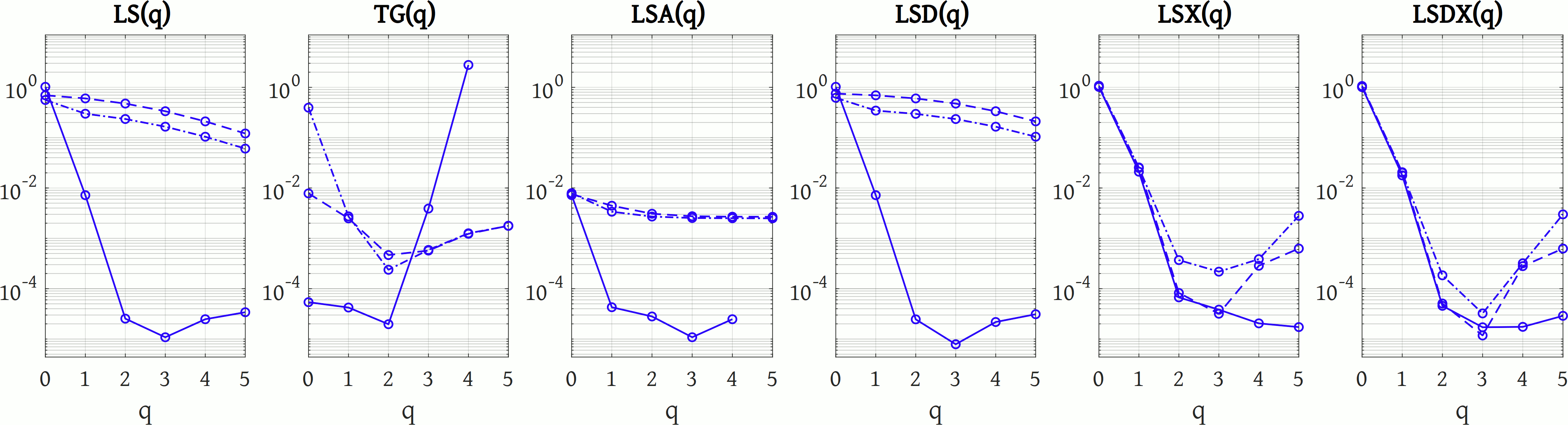
(b) HARCO meshes

Figure 24: Average normalised errors of several gradient schemes, as a function of the exponent $q$, for computing the gradient of the azimuthally-varying function (33) on the $l=6$ HARC 22(a) and HARCO 22(b) grids. The errors on structured grids are drawn with continuous lines, those on orderly triangulated grids with dashed lines, and those on randomly triangulated grids with dash-dot lines.

Figure 24 shows the normalised (by the new $G$) errors on level $l=6$ of the HARC and HARCO meshes. Results are given only for the cases where the 8-byte calculations are arithmetically stable. This appears to be an easier test case for the gradients, as the normalised errors are about an order of magnitude smaller than those for the radial function 32. The accuracy improvement compared to the differentiation of the radial function is particularly large for the extended-stencil gradients LSX and LSDX with high $q$ exponents on the randomly triangulated grids. On the other hand, the accuracy of the nearest-neighbour stencil gradients LS and LSD on the triangle grids is still terrible.

8.2 Numerical stability

As mentioned, the results plotted in Fig. 25 revealed that some gradients exhibited a numerical instability at finer meshes. The instability disappeared when the calculations were performed in higher precision arithmetic, which indicates that roundoff errors play a role. Factors that were observed to either trigger or aggravate the instability are the grid fineness and the weighting exponent $q$. Of course, it is reasonable to assume that the high aspect ratio is also a necessary ingredient, since no such instabilities were observed in the tests of Sec. 7.

When it comes to least-squares methods, it is well known [34] that solution of the over-determined system by means of the normal equations, which is what is practiced in the present work, can lead to numerical instabilities. For orthogonal projections (Eq. (11))) our solution method, Eq. (10), gives $\mathbf{x}=(\mathbf{A}^{\mathrm{T}}\mathbf{A})^{-1}\mathbf{A}^{\mathrm{T}}\mathbf{y}$. These operations return $\mathbf{x}$ but can amplify round-off errors by a factor of $\kappa(\mathbf{A})^{2}$, where $\kappa(\mathbf{A})$ is the condition number of the matrix $\mathbf{A}$, so depending on this number the error of the calculation can be very large [34]. The remedy, in the orthogonal projection case, is to do a QR or SVD decomposition of the matrix $\mathbf{A}$ which leads to alternative algorithms [34] that do not solve the normal equations but involve cancellations between orthogonal matrices done beforehand in exact arithmetic (not applicable in oblique projection cases). These algorithms amplify roundoff errors in $\mathbf{A}$ and $\mathbf{y}$ only by a factor $\kappa(\mathbf{A})$ and are therefore much more stable.

The effect of the condition number on the accuracy of least squares gradients has not been thoroughly investigated in the literature, but some studies do exist. In [33] a least-squares procedure was devised to construct gradients of first- and higher-order accuracy, using SVD; the higher-order variants had much larger condition numbers (up to $10^{12}$ reported for aspect ratios of 1000), but this could be brought down significantly by scaling the columns of the matrix $\mathbf{A}$. Seo et al. [36] compared what is effectively our LS(2) and LSX(2) gradients, computed via solution of the normal equations, against a couple of Green-Gauss gradients. Tests were performed on grids of aspect ratios up to 500, and it was found that there is a positive correlation between the condition number $\kappa(\mathbf{A}^{\mathrm{T}}\mathbf{A})\sim\kappa(\mathbf{A})^{2}$ and the gradient error. Condition numbers of nearly up to 20,000 were reported for the product $\mathbf{A}^{\mathrm{T}}\mathbf{A}$ of the LS(2) gradient, but those of the LSX(2) gradient were much smaller; this gave rise to the idea of using $\kappa(\mathbf{A}^{\mathrm{T}}\mathbf{A})$ as a criterion for switching between the cheaper LS(2) gradient and the more expensive LSX(2) gradient.

To find out whether our instability is related to the normal equations, we repeated the LSA gradient calculations (the most unstable ones) using the SVD algorithm instead. The DGELSD subroutine of the LAPACK [38] library was used for this purpose; it returns also the singular values of $\mathbf{A}$, from which $\kappa(\mathbf{A})$ can be easily computed as the ratio of largest to smallest singular value. The LSA gradient can be brought into the form (11) with $\mathbf{A}=\mathbf{D}^{\frac{1}{2}}\mathbf{R}$ and $\mathbf{y}=\mathbf{D}^{\frac{1}{2}}\mathbf{b}$, in the notation of Sec. 2.1 (Eqs. (7) and (8)), where $\mathbf{D}^{\frac{1}{2}}$ is a diagonal matrix with elements $D_{ff}=(\|\underline{S}_{f}\|/\|\underline{R}_{f}\|^{q})^{\frac{1}{2}}$. Unfortunately, using the SVD did not improve the stability: the results were exactly the same as for the normal equations. Furthermore, while the condition numbers $\kappa(\mathbf{A})$ were indeed found to increase with increasing $q$ (e.g. $\kappa(\mathbf{A})$ has mean values of roughly 1, 32 and 1000 for $q$ = 1, 2 and 3, respectively, and the maximum $\kappa(\mathbf{A})$ are not much larger than the mean), they were not large enough to explain the instability (even the LSA(3) became unstable under certain conditions, described below). Finally, the condition numbers were found to be nearly independent of the grid fineness, whereas the instability shows a strong dependence on it.

So, the origin of the instability must be sought elsewhere. In fact, experiments showed a very strong dependence on the algorithm used to calculate the cell centroids. For all the experiments of Sec. 7, and for the triangular grid experiments of Sec. 8, the coordinates of the cell centroids $\underline{C}_{0}=(x_{0},y_{0})$ were calculated with formulae derived using the Gauss theorem:

$$x_{0}\;=\;\frac{1}{\Omega_{0}}\iiint_{\Omega_{0}}x\,\mathrm{d}\Omega\;=\;\frac{1}{\Omega_{0}}\iint_{S_{0}}\frac{x^{2}}{2}\,\hat{\underline{e}}_{x}\cdot\mathrm{d}\underline{S}\;=\;\frac{1}{6\Omega_{0}}\sum_{f=1}^{4}(x_{f,1}^{2}+x_{f,1}x_{f,2}+x_{f,2}^{2})\hat{\underline{e}}_{x}\cdot\underline{S}_{f}$$ (34)

and similarly for $y_{0}$, where $\Omega_{0}$ and $S_{0}$ are the volume and bounding surface of the cell, $\hat{\underline{e}}_{x}$ is the unit vector in the $x$ direction, and $x_{f,1}$ and $x_{f,2}$ are the $x$-coordinates of the two vertices of face $f$. Another method that was tried was simply averaging the coordinates of the cell’s vertices. Strictly speaking, this is not equal to the geometric centroid, but the two converge with grid refinement on structured quadrilateral grids such as the present ones. The great difference in stability resulting from these two methods can be seen in Fig. 25. The HARC and HARCO quadrilateral grid results of Sec. 8.1 were obtained with the simple averaging method. Yet another method that was tried was splitting each quadrilateral into two triangles, and computing the centroid as an area-weighted average of the centroids of the two triangles. In exact precision arithmetic, this method would give exactly the same result as formula (34). This method resulted in better stability than Eq. 34, but worse than simple averaging.

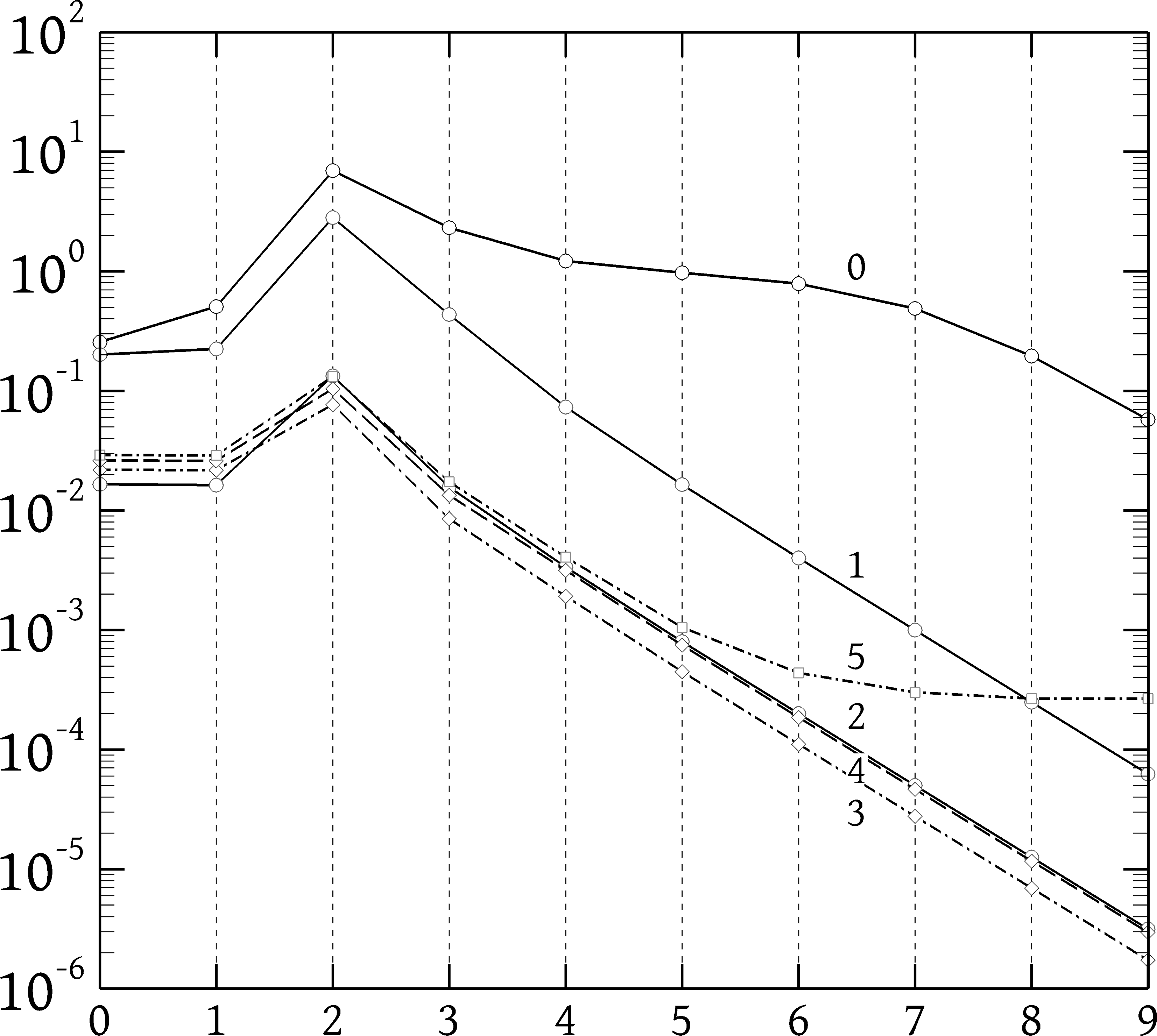
(a)

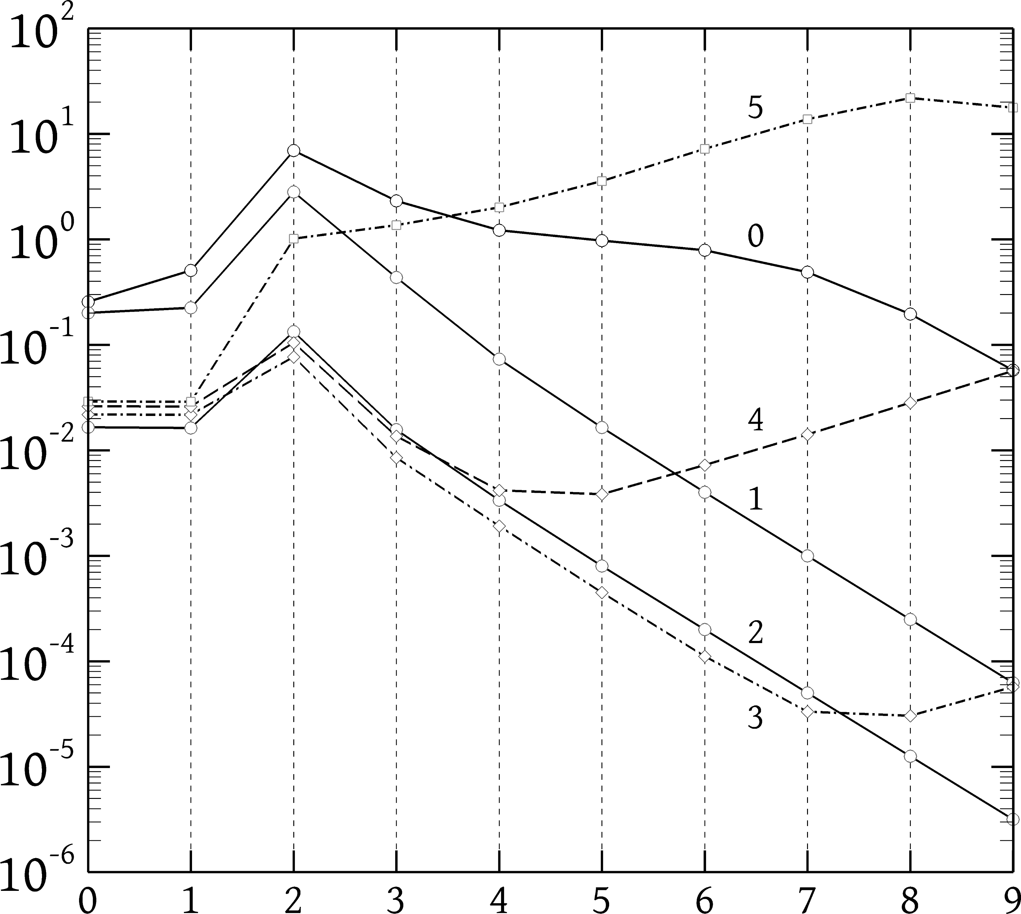
(b)

Figure 25: Mean normalised errors of the LS($q$) gradients, with $q$ indicated on each curve, as a function of the refinement level $l$, on the HARC quadrilateral grids. 25(a) Cell centroids calculated as simple averages of the cells’ nodes. 25(b) Cell centroids calculated via formulae (34). The function (32) is differentiated. All calculations were performed in 8-byte precision.

To provide a better feel for the potential severity of this instability, Fig. 26 shows the errors of all gradients, with $q=3$, on the HARCO quadrilateral grids, for both the radial and azimuthal functions, with centroids calculated via (34). To better test the stability of the gradients, two additional refinement levels are included ($l=10$ and $11$, with $2048$ and $4096$ cells in each direction, respectively). Both 8- and 10-byte calculations are included, so that the effects of the instability can be evident. The instability is more prominent in the radial function case, but the azimuthal function case is not immune to it either. In the radial function case, the 8-byte LSA gradient becomes unstable already at level $l=4$, and even the 10-byte version does not manage to remain stable all the way down to the finest grid. All the other gradients become unstable at $l=8$, except the TG gradient which, although stable, has a huge error.

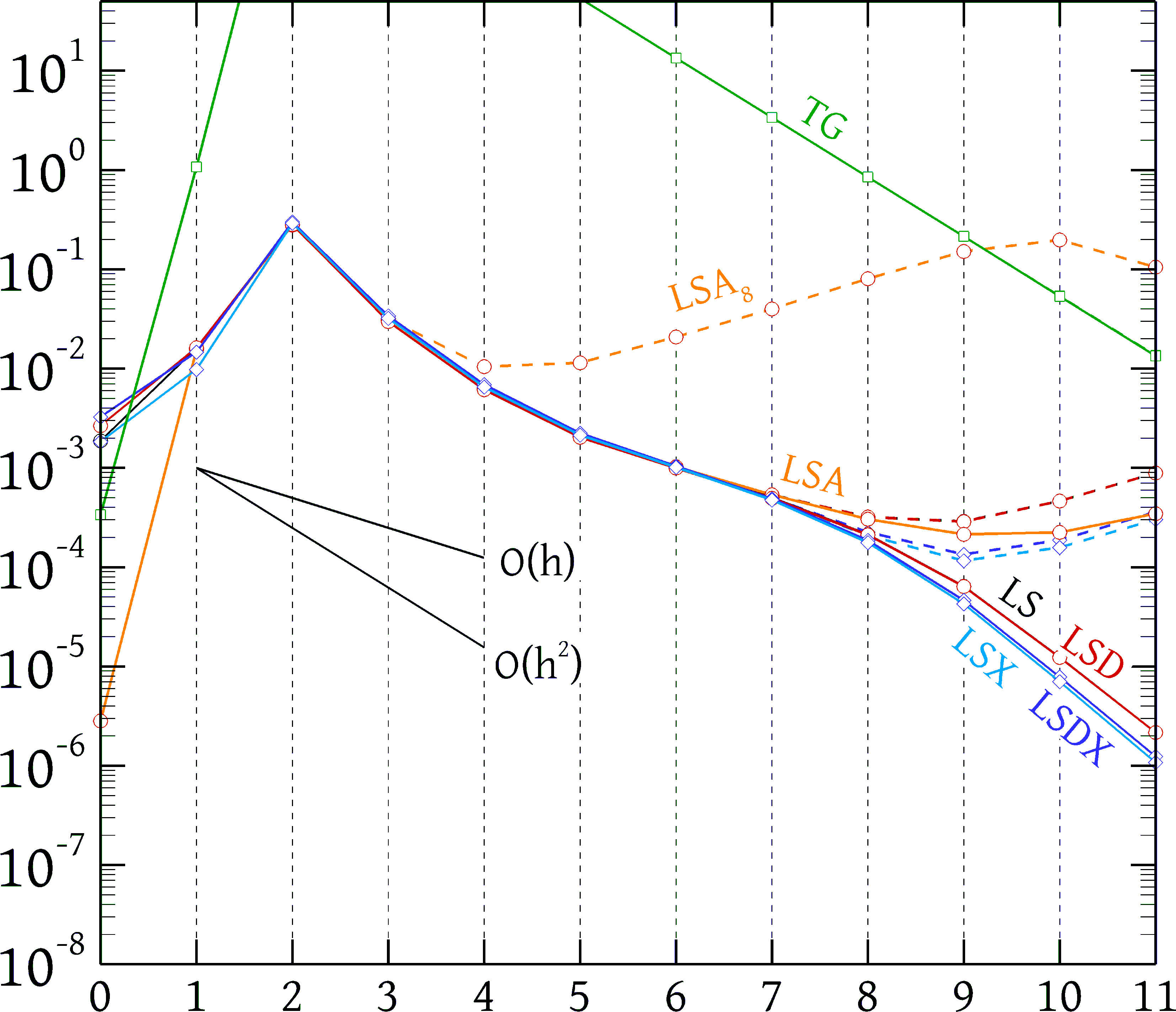
(a) Radial function (32)

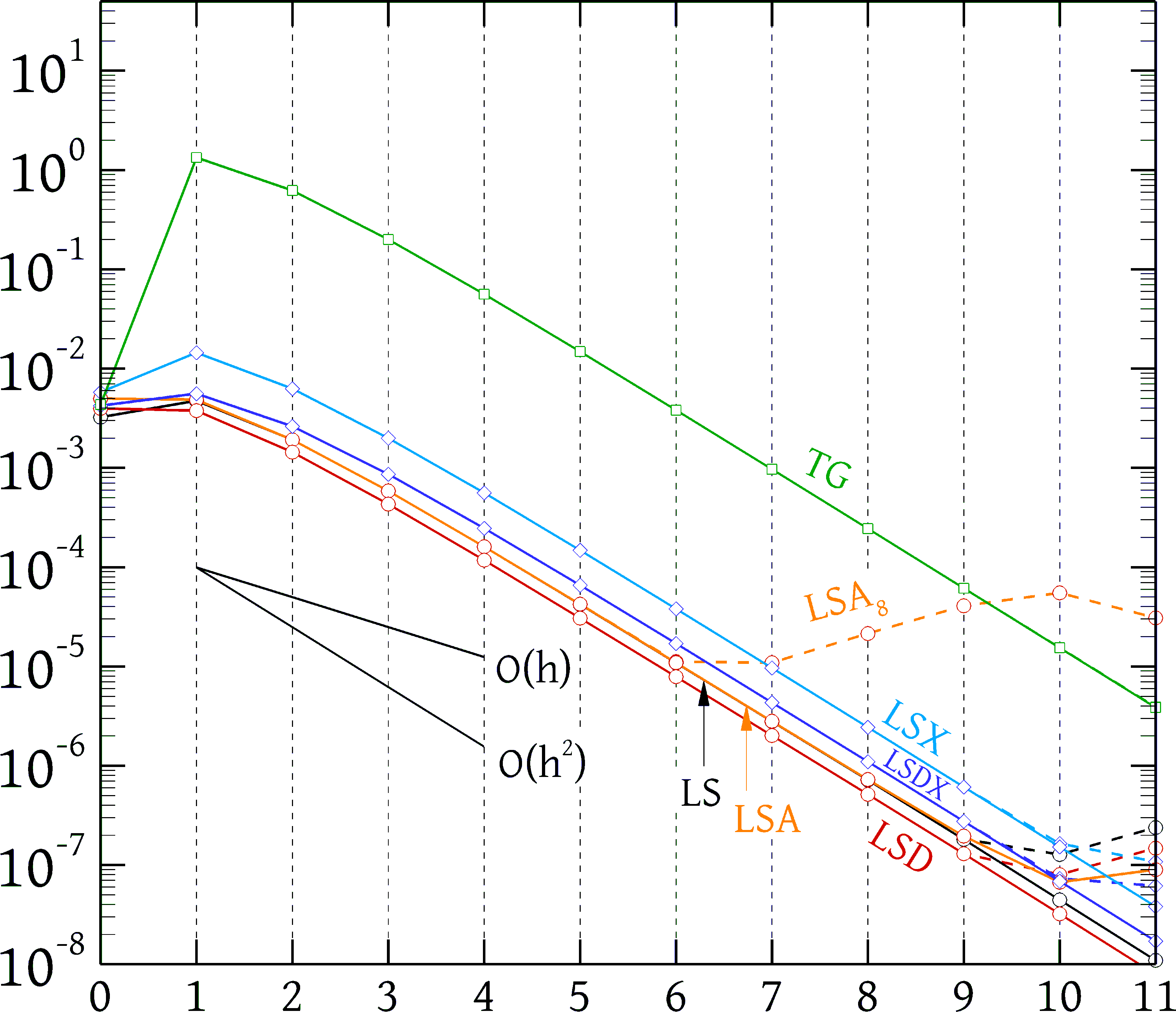
(b) Azimuthal function (33)

Figure 26: Mean normalised errors of the LS(3), LSD(3), LSA(3), TG(3), LSX(3) and LSDX(3) gradients on the quadrilateral HARCO grids. Dashed lines: 8-byte calculations; continuous lines: 10-byte calculations.

To locate the source of the instability, we performed downscaling tests [39], which use only a tiny fraction of the grid (the stencil of Fig. 19) and allow refinement down to very fine levels. The cell configuration was representative of the HARC quadrilateral grid, as in Fig. 19, and the radial function was considered. The findings that helped pinpoint the source of the instability are the following.

1. If all calculations are performed in quadruple (16 byte) precision, then the instabilities vanish.

2. The formula (34), in 8-byte arithmetic, which results in more intense instability, introduces larger misalignment between the ideally colinear nodes $\underline{C}_{1}$, $\underline{C}_{0}$ and $\underline{C}_{3}$ (Fig. 19), than the more stable node averaging method.

3. If only the centroid calculations are performed in 8-byte precision and all other operations (calculation of the $\underline{R}_{f}$ and $\underline{V}_{f}$ vectors, assembly and solution of the normal equations etc.) are performed in 16-byte precision, then there is no improvement in stability compared to the case that all calculations are performed in 8-byte precision.

4. Misalignment between the colinear centroids correlates with the production of a large spurious azimuthal component of the gradient, whereas the error in the radial component remains small.

Observation 3 is important because it means that the errors that we labeled as stability errors thus far, seen in Figs. 20, 25 and 26, are actually not round-off errors but truncation errors, since they occur even if all gradient-related operations are essentially exact (quadruple precision). Calculation of the cell centroids cannot be considered to be part of the gradient calculation. If the gradient schemes have a small truncation error then they should accurately compute the gradient whether the centroids are aligned or not. So, all these observations taken together point to the following explanation for the instabilities.

To keep things simple, consider the model stencil of Fig. 27. Grid curvature is not necessary for the instability to occur, so it has been omitted. We have perturbed only one centroid, $\underline{C}_{3}$, a distance $\delta$ horizontally. The $\underline{R}_{f}$ vectors are therefore $\underline{R}_{1}=(0,-h)$, $\underline{R}_{2}=(Ah,0)$, $\underline{R}_{3}=(\delta,h)$ and $\underline{R}_{4}=(-Ah,0)$. Hence the $\mathbf{R}$ and $\mathbf{V}$ matrices for the LS($q$) gradient are:

$$\mathbf{R}\;=\;\begin{bmatrix}0&Ah&\delta&-Ah\\ -h&0&h&0\end{bmatrix}^{\mathrm{T}}$$ (35)

$$\mathbf{V}\;=\;\begin{bmatrix}0&A^{1-q}h^{1-q}&\delta h^{-q}&-A^{1-q}h^{1-q}\\ -h^{1-q}&0&h^{1-q}&0\end{bmatrix}^{\mathrm{T}}$$ (36)

where, for simplicity, we assumed in $\underline{V}_{3}$ that $\|\underline{R}_{3}\|\approx h$.

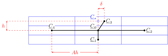
Figure 27: A model stencil for a theoretical analysis of the instability.

Now, assume that we are differentiating a radially-varying function such as (32), with the origin of the polar coordinate system located on the line joining $\underline{C}_{0}$ and $\underline{C}_{1}$, as in Fig. 19. Then $\phi_{2}=\phi_{4}$ and the vector $\mathbf{b}$ in Eq. (10) is ($\phi_{f}$ being short for $\phi(\underline{C}_{f})$):

$$\mathbf{b}\;=\;\left[\;\phi_{1}-\phi_{0}\quad 0\quad\phi_{3}-\phi_{0}\quad 0\;\right]^{\mathrm{T}}$$ (37)

Then, the solution (10) to the system (9) is:

$$\mathsf{x}_{1}\; =\;\frac{\delta(\phi_{3}-2\phi_{0}+\phi_{1})}{4A^{2-q}h^{2}+\delta^{2}}$$ (38)

$$\mathsf{x}_{2}\; =\;\frac{4A^{2-q}h^{2}}{4A^{2-q}h^{2}+\delta^{2}}\;\frac{\phi_{3}-\phi_{1}}{2h}\;+\;\frac{\delta^{2}}{4A^{2-q}h^{2}+\delta^{2}}\;\frac{\phi_{0}-\phi_{1}}{h}$$ (39)

($\mathsf{x}_{1}$ and $\mathsf{x}_{2}$ must not be confused with the $x$ coordinate; they are the two components of the vector $\mathbf{x}$ of Eq. (10) which are intended to hold approximations to $\partial\phi/\partial x$ and $\partial\phi/\partial y$, respectively). It is noted that if $\phi$ were a linear function, $\phi=\phi_{0}+Gy$ (it must have this form for $\phi(\underline{C}_{2})$ to equal $\phi(\underline{C}_{4})$), then $\mathsf{x}_{1}=0$ and $\mathsf{x}_{2}=G$, which are the exact values. If $\phi$ is a non-linear, radial function ($\phi=\phi(r)$) but $\delta=0$, then $\mathsf{x}_{1}=0$ (the exact value) and $\mathsf{x}_{2}=(\phi_{3}-\phi_{1})/2h$ (a very good approximation).

Now suppose that $\phi=\phi(r)$ and $\delta\neq 0$. The value of $\mathsf{x}_{2}$ can be seen from (39) to lie between $(\phi_{3}-\phi_{1})/2h$ and $(\phi_{0}-\phi_{1})/h$; when $\delta$ is small such that $\delta^{2}\ll 4A^{2-q}h^{2}$, then $\mathsf{x}_{2}\rightarrow(\phi_{3}-\phi_{1})/2h$, which, in this case, is a good approximation to $\partial\phi/\partial y$. At the other extreme, when $\delta^{2}\gg 4A^{2-q}h^{2}$ then $\mathsf{x}_{2}\rightarrow(\phi_{0}-\phi_{1})/h$, which is still a good approximation to $\partial\phi/\partial y$. In general, no matter what the value of $\delta$, $\mathsf{x}_{2}$ will return acceptable approximations to $\partial\phi/\partial y$.

However, this is not the case for $\mathsf{x}_{1}$, the approximation to the azimuthal component of the gradient, which should ideally be zero. Let $\bar{\phi}_{*}$ be the linearly extrapolated value of $\phi$ at point $\underline{C}_{*}=(0,h)$ (Fig. 27), assuming $\partial\phi/\partial y\approx(\phi_{0}-\phi_{1})/h$:

$$\bar{\phi}_{*}\;=\;\phi_{0}\;+\;\frac{\phi_{0}-\phi_{1}}{h}\,h\;=\;2\phi_{0}\;-\;\phi_{1}$$ (40)

Noting that $\phi_{3}-2\phi_{0}+\phi_{1}=\phi_{3}-\bar{\phi}_{*}$, Eq. (38) can be written in a form similar to (39) as

$$\mathsf{x}_{1}\;=\;\frac{4A^{2-q}h^{2}}{4A^{2-q}h^{2}+\delta^{2}}\;0\;+\;\frac{\delta^{2}}{4A^{2-q}h^{2}+\delta^{2}}\;\frac{\phi_{3}-\bar{\phi}_{*}}{\delta}$$ (41)

The first term on the right-hand side is zero, but it has been included because it represents the finite difference $(\phi_{2}-\phi_{4})/(2Ah)=0$. Thus, the value of $\mathsf{x}_{1}$ lies somewhere between the finite difference $(\phi_{2}-\phi_{4})/(2Ah)$ and the finite difference $(\phi_{e}-\bar{\phi}_{*})/\delta$. To which one it is closer is determined by the relative magnitude of $\delta^{2}$ compared to $4A^{2-q}h^{2}$. Inverse-distance weighting can lead to the contributions of points $\underline{C}_{2}$ and $\underline{C}_{4}$ to the LS gradient being suppressed, if the aspect ratio $A$ and the weight exponent $q$ are large enough so that $4A^{2-q}h^{2}<\delta^{2}$. In that case $\mathsf{x}_{1}$ will be closer to $(\phi_{e}-\bar{\phi}_{*})/\delta$. In the extreme case of very large $A$ and $q$ the contributions of $\underline{C}_{2}$ and $\underline{C}_{4}$ are completely eliminated and we are left only with $\underline{C}_{0}$, $\underline{C}_{1}$ and $\underline{C}_{3}$. These are three non-colinear points, so the system (7) is not overdetermined but has a unique solution. This solution is the same as that of Eqs. (41) and (39) if we set $4A^{2-q}h^{2}\rightarrow 0$:

$$\mathsf{x}_{1}\;=\;\frac{\phi_{3}-\bar{\phi}_{*}}{\delta}\qquad\qquad\mathsf{x}_{2}\;=\;\frac{\phi_{0}-\phi_{1}}{h}$$ (42)

As mentioned, the error is small for $\mathsf{x}_{2}$. However, it can be huge for $\mathsf{x}_{1}$; the problem is that, if $\delta\rightarrow 0$, $\phi_{3}$ tends to the value $\phi(\underline{C}_{*})$, which is different from $\bar{\phi}_{*}$ because the latter is just an extrapolated value. Hence, as $\delta\rightarrow 0$ the difference $\phi_{3}-\bar{\phi}_{*}$ remains finite and the ratio $\mathsf{x}_{1}=(\phi_{3}-\bar{\phi}_{*})/\delta$ goes to infinity.

For a quantitative estimate of this error, we can expand $\phi(r)$ as Taylor series in $(x,y)$ coordinates around point $\underline{C}_{0}$. If $\partial\phi/\partial x=0$ and $\partial\phi/\partial y=G$ is the exact gradient, it is not hard to show that also $\partial^{2}\phi/\partial x^{2}=G/r$, $\partial^{2}\phi/\partial y^{2}=\mathrm{d}^{2}\phi/\mathrm{d}r^{2}$ and $\partial^{2}\phi/\partial x\partial y=0$ (all derivatives evaluated at $\underline{C}_{0}$). Expanding $\phi_{1}$ and $\phi_{3}$ thus we obtain

$$\bar{\phi}_{*}\; =\;\phi_{0}\;+\;Gh\;-\;\frac{1}{2}\phi^{\prime\prime}h^{2}$$ (43)

$$\phi_{3}\; =\;\phi_{0}\;+\;Gh\;+\;\frac{1}{2}\phi^{\prime\prime}h^{2}\;+\;\frac{1}{2r}G\delta^{2}$$ (44)

where $\phi^{\prime\prime}=\partial^{2}\phi/\partial r^{2}$. It is obvious that these two values do not converge if $\delta\rightarrow 0$. Substituting in (42) we get for $\mathsf{x}_{1}$:

$$\mathsf{x}_{1}\;=\;\frac{\phi^{\prime\prime}h^{2}}{\delta}\;+\;\frac{G\delta}{2r}$$ (45)

If $\delta\rightarrow 0$ then the second term on the right-hand side tends to zero, but the first term tends to infinity, hence we get very large errors in the azimuthal component of the gradient. It is noteworthy that, perhaps counterintuitively at first sight, the smaller $\delta$ is, i.e. the better the alignment of the cell centroids, the larger the error; it is only when $\delta$ is exactly zero that the error becomes zero too. In practice though, we observed that better alignment of the centroids results in smaller error (e.g. node averaging vs. the formulae (34)). This is because if $\delta$ becomes too small then the assumption on which Eq. (45) is based, that $\underline{C}_{2}$ and $\underline{C}_{4}$ do not contribute to the gradient, is invalidated. As seen from Eq. (41), formula (45) is an accurate approximation to the solution $\mathsf{x}_{1}$ if $\delta^{2}\gg 4A^{2-q}h^{2}$. So, the peak error would be expected to occur roughly at a value $\delta_{*}$ for which $\delta_{*}^{2}=4A^{2-q}h^{2}$, or

$$\delta_{*}\;=\;2AhA^{-q/2}\qquad\text{or}\qquad\tilde{\delta}_{*}\;\equiv\;\frac{\delta_{*}}{2Ah}\;=\;A^{-q/2}$$ (46)

where $\tilde{\delta}_{*}$ is a non-dimensional version of $\delta_{*}$ that compares it to the distance $2Ah$ between $\underline{C}_{2}$ and $\underline{C}_{4}$. If $\delta$ is increased beyond $\delta_{*}$ then equation (45) describes the error well, but since $\delta$ is increasing, the error is falling; on the other hand, if $\delta$ is decreased below $\delta_{*}$, then Eq. 45 does not describe the error accurately, and $\mathsf{x}_{1}$ becomes increasingly dominated by the finite difference $(\phi_{2}-\phi_{4})/(2Ah)$, which has a small error (zero, in this case).

This theoretical analysis is confirmed by the downscaling tests. Figure 28 shows results of such tests, which include grid curvature as in Fig. 19, with $A=1000$ and $r=1$. The maximum errors do indeed occur at about $\delta_{*}$. The larger the values of $q$, the larger the possible errors. The errors can be huge for $q=4$ and $5$, and large for $q=3$. Use of $q\leq 2$ is recommended for safety. The errors decrease with grid refinement; in Figs. 25 and 26 the errors are seen to actually increase with refinement up to a certain grid level, and decrease subsequently. This can be attributed to the fact that grid refinement also affects $\delta$, and can bring it closer to $\delta_{*}$.

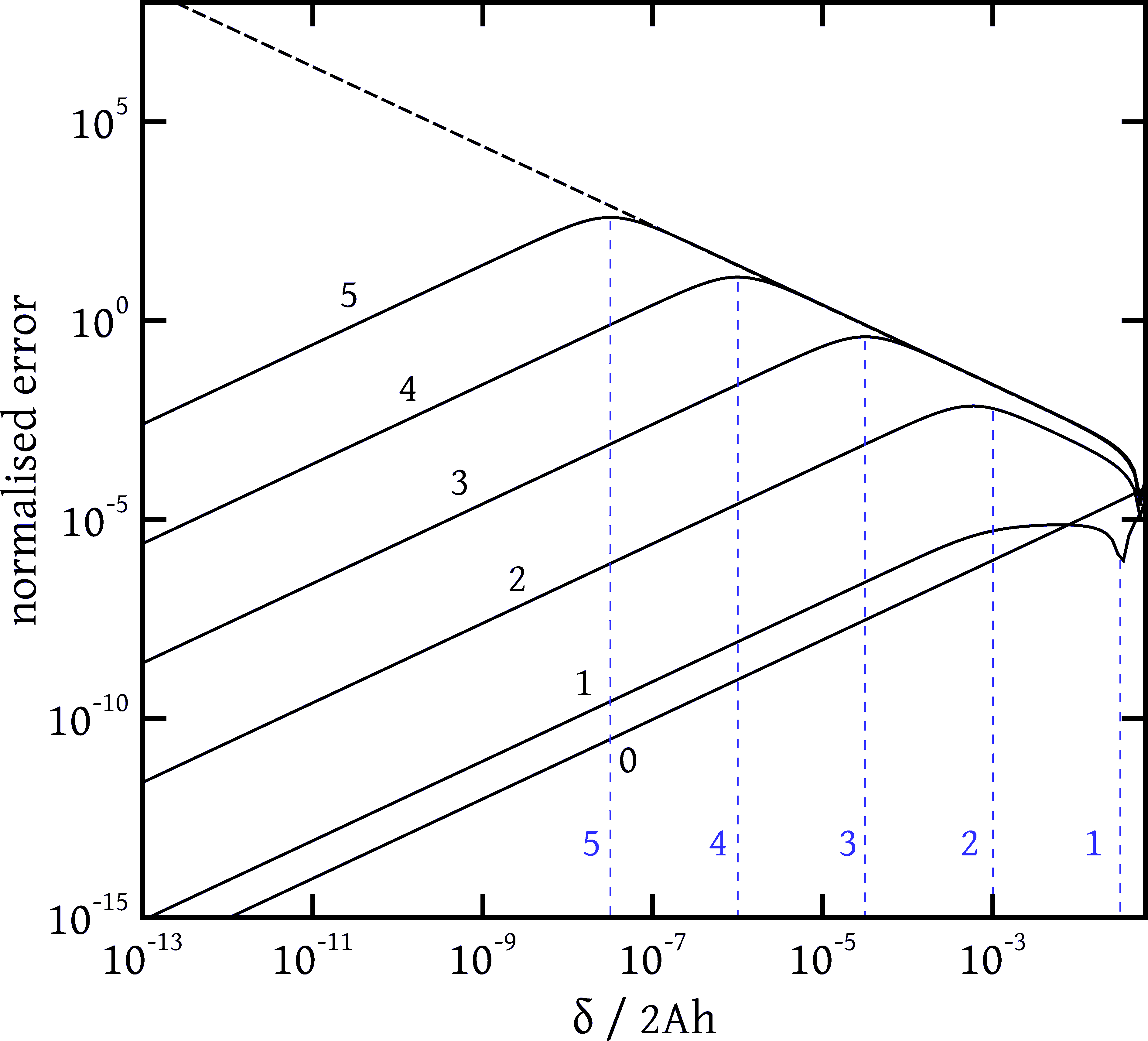
(a) $l=5$

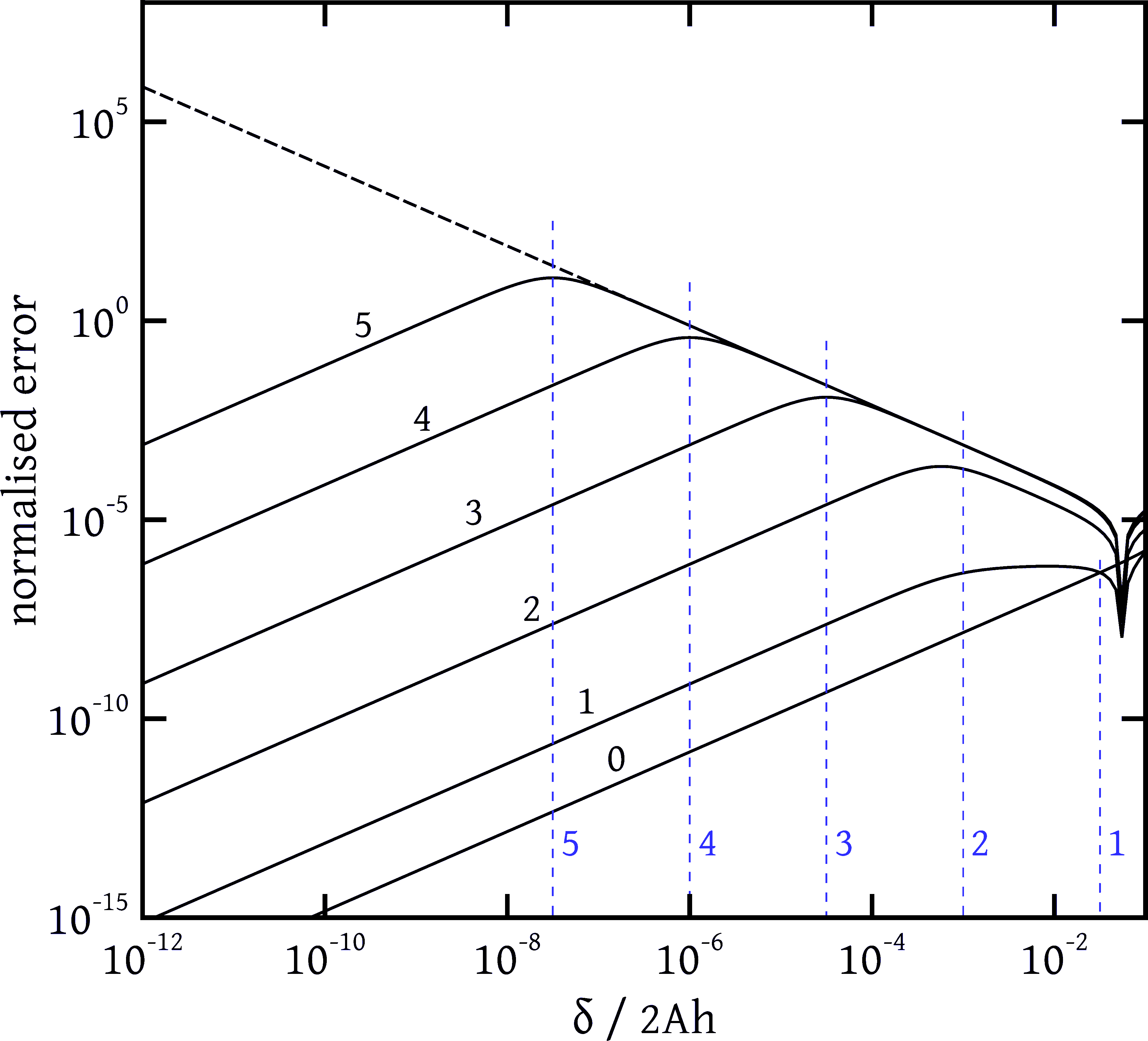
(b) $l=10$

Figure 28: Solid lines: normalised errors ($|\mathsf{x}_{1}|/G$) of the LS($q$) gradients ($q$ shown next to each curve) as a function of the horizontal perturbation $\delta$ of point $\underline{C}_{3}$, in downscaling tests (Fig. 19) with $A=1000$, at $\underline{C}_{0}=(r=1,\theta=0)$. The function (32) is differentiated ($G=1679.9$, $\phi^{\prime\prime}=-1.0235\cdot 10^{7}$). Dashed back line: the error predicted by Eq. (45). Vertical blue dashed lines: the values of $\delta_{*}$ (Eq. (46)) for each $q$. Left plot 28(a): grid level $l=5$ ($h=8\cdot 10^{-6}$). Right plot: grid level $l=10$ ($h=2.5\cdot 10^{-7}$).

9 Conclusions

The current study presented a general framework for formulating gradient reconstruction schemes based on the solution, via projection onto a selected subspace, of an over-determined system, derived from Taylor series expansion of the differentiated variable in a neighbourhood of cells. Two particular sub-families were the focus of investigation: least-squares gradients, based on orthogonal projection, and Taylor-Gauss gradients, based on oblique projection on a subspace formed by the cells’ face normal vectors, which turns out to be equivalent to a self-corrected Green-Gauss gradient. Of course, these sub-groups do not exhaust the general framework, and other projection subspaces, possibly even based on vectors that depend on the solution and vary dynamically, may be devised and tested in the future.

The hope going into this study was to find a gradient scheme that performs well under all circumstances, with the ultimate goal of finding a gradient that can be safely applied in general purpose finite volume solvers, without worrying about the particularities of each given problem. Eventually, each of the schemes tested turned out to have some advantages and disadvantages.

The LS($q$) gradients usually perform well on quadrilateral grids with $q=2$ or $3$. On triangular grids, their performance suffers but can be greatly improved by extending the stencil (LSX($q$) gradients). On high aspect ratio quadrilateral grids, the weighting exponent $q$ should not be increased beyond 2, or 3 with some caution, if the risk of instability is to be avoided – however, the value $q=0$ should also not be used.

The LSA and LSD gradients were designed to offer improved performance on grids with directional clustering, compared to the LS gradients. The LSD gradient is slightly more expensive than the LSA, but it has the advantage that it can be used also with extended stencils; indeed, the LSDX gradient was the most accurate in most cases (followed closely by LSX). Furthermore, the LSD gradient is more stable than the LSA on high aspect ratio grids.

The TG and TGI gradients usually performed on par with the compact least squares gradients, LS, LSA and LSD, or even outperformed them (on the elliptic and locally refined grids). However, their inapplicability to extended stencils significantly limits their accuracy on triangular grids. Furthermore, they performed very poorly on the HARCO grids, unless $q=0$ or $q=1$ was used.

In general, on the grids of Sec. 7 most gradients would perform satisfactorily, even though some are better than others. An exception may be triangular grids, on which extended stencils should be used. For more complex unstructured grids with varying types of cell geometry, the technique proposed in [36] for switching between compact and extended stencils may be useful. On the other hand, on high aspect ratio grids such as those of Sec. 8, which present extreme cases, more caution is warranted, as any one of the gradients we examined could fail catastrophically under some set of conditions. High aspect ratio combined with relatively high distance weighting exponent $q$ can give rise to the instability discussed in Sec. 8.2, particularly for the LSA gradient, but also for the others. Even without this instability, the TG gradient fails catastrophically on quadrilateral HARCO meshes if $q>1$. The same is true also of the LSX and LSDX gradients on randomly triangulated grids for $q>3$. The LS and LSD gradients have quite poor accuracy on triangulated high aspect ratio grids, for all values of $q$, although there is a slight improvement as $q$ is increased.

Summarising, for normal aspect ratio grids such as those of Sec. 7, if the grid is composed of quadrilaterals, the TG(2) gradient may be a good choice that combines accuracy with low computational cost; it inherently accounts for directional clustering, and offers 2nd order accuracy at boundaries. If the grid is composed of triangles, then the LSDX(3) (or LSX(3)) gradient would be a better choice. The LSDX(3) gradient would also be a good choice for quadrilateral grids, if the additional computational cost can be afforded, as it proved to be the most accurate on distorted grids such as that of Fig. 3(c). For better efficiency, one could use a criterion to switch between compact and extended stencils such as that used in [36]. On high-aspect ratio grids, if they are composed of quadrilaterals, the LS(2) gradient is a good choice; LS(3) would be more accurate, but it is best to avoid large $q$ exponents due to the fear of instability. If the grid is triangular, then LSX(2) should be preferred instead. Although we did not test this idea, theoretically on HARC quadrilateral grids one could use the LS(3) gradient to benefit by its higher accuracy at boundaries, and mitigate the danger of instability by multiplying the weight vectors $\underline{V}_{2}$ and $\underline{V}_{4}$ (Fig. 19) by appropriate factors so that their magnitudes do not become too small in comparison to those of $\underline{V}_{1}$ and $\underline{V}_{3}$ (or, equivalently, by applying a smaller $q^{\prime}<q$ exponent in the directions 2 and 4 than the $q=3$ exponent in the directions 1 and 3).

Finally, it must be noted that the present study is a necessary first step for assessing these gradient schemes for the purpose of employing them in Finite Volume Methods, but this must be followed by a study where they are tested in the actual FVM solution of partial differential equations. The present study evaluated the truncation error of the gradients schemes themselves, but how this will affect the truncation error of the overall FVM and the discretisation error of the solution remains to be seen. For example, the property of gradients such as the LS(3), TG(2) etc. that, on quadrilateral grids, they retain second-order accuracy even at boundary cells, may reduce the discretisation error throughout the domain, as this error is produced locally at sites of high truncation error and convected and diffused along with the flow [40, 41]. Furthermore, the choice of gradient scheme may have an impact on the iterative convergence of the algebraic solver [42]. Such a study is planned for the future.

Appendix

In this appendix, it will be shown that the second term on the right-hand side of Eq. (27) is equal to the identity tensor. Consider a Cartesian coordinate system with origin at $\underline{C}_{0}$, with $x_{i}$ being the $i$-th coordinate direction and $\hat{\underline{e}}_{i}$ the corresponding unit vector. Then

$$\nabla\cdot(x_{i}\hat{\underline{e}}_{j})\;=\;\delta_{ij}\;\Rightarrow\;\int_{\Omega_{0}}\nabla\cdot(x_{i}\hat{\underline{e}}_{j})\mathrm{d}\Omega\;=\;\int_{\Omega_{0}}\delta_{ij}\mathrm{d}\Omega\;=\;\delta_{ij}\,\Omega_{0}$$ (47)

The integral of Eq. (47) can also be evaluated using the divergence (Gauss) theorem:

$$\int_{\Omega_{0}}\nabla\cdot(x_{i}\hat{\underline{e}}_{j})\mathrm{d}\Omega\;=\;\int_{S_{0}}x_{i}\hat{\underline{e}}_{j}\cdot\hat{\underline{n}}\,\mathrm{d}S\;=\;\sum_{f}\hat{\underline{e}}_{j}\cdot\hat{\underline{n}}_{f}\int_{S_{f}}x_{i}\,\mathrm{d}S\;=\;\sum_{f}\hat{\underline{e}}_{j}\cdot\underline{S}_{f}R_{f,i}$$ (48)

where $S_{0}$ is the surface of cell $\Omega_{0}$, $\mathrm{d}S$ is an infinitesimal element of that surface, and $\hat{\underline{n}}$ is the outward normal unit vector, which is constant and equal to $\hat{\underline{n}}_{f}$ over each face $f$. In the last equality of Eq. (48) we have used that $\int_{S_{0}}x_{i}\,\mathrm{d}S=S_{f}c_{f,i}$, with $c_{f,i}$ being the $i$-th component of the centroid $\underline{c}_{f}$, by definition of the centroid. The latter also equals $R_{f,i}$, the $i$-th component of $\underline{R}_{f}=\underline{c}_{f}-\underline{C}_{0}$, because $\underline{C}_{0}=\underline{0}$ is the coordinates’ origin . Thus Eq. (48) becomes $\sum_{f}S_{f,j}R_{f,i}$, i.e. the $(j,i)$ component of the tensor $\sum_{f}\underline{S}_{f}\underline{R}_{f}$. This is equal to $\delta_{ji}\Omega_{P}$, the $(j,i)$ component of the tensor $\Omega_{P}\underline{\underline{I}}$, by Eq. (47). Thus the tensors $\Omega_{P}\underline{\underline{I}}$ and $\sum_{f}\underline{S}_{f}\underline{R}_{f}$ are identical, having all their components equal, which is the sought result. Placing the origin elsewhere ($\underline{C}_{0}\neq\underline{0}$) does not change the result, because $\sum_{f}\underline{S}_{f}\underline{C}_{0}=(\sum_{f}\underline{S}_{f})\underline{C}_{0}=\underline{0}\underline{C}_{0}=\underline{\underline{0}}$.

References

- [1] P. Traoré, Y. M. Ahipo, C. Louste, A robust and efficient finite volume scheme for the discretization of diffusive flux on extremely skewed meshes in complex geometries, J. Comput. Phys. 228 (2009) 5148–5159.
- [2] I. Demirdžić, On the discretization of the diffusion term in finite-volume continuum mechanics, Numer. Heat Transfer B 68 (2015) 1–10.
- [3] A. Jalali, M. Sharbatdar, C. Ollivier-Gooch, An efficient implicit unstructured finite volume solver for generalised Newtonian fluids, International Journal of Computational Fluid Dynamics 30 (3) (2016) 201–217. doi:10.1080/10618562.2016.1188202.
- [4] J. H. Ferziger, M. Peric, Computational methods for fluid dynamics, 3rd Edition, Springer, 2002.
- [5] A. M. Afonso, M. S. N. Oliveira, P. J. Oliveira, M. A. Alves, F. T. Pinho, The finite volume method in computational rheology, in: Finite-Volume Methods – Powerful Means of Engineering Design, In-Tech Open Publishers, 2012, Ch. 7, pp. 141–170.
- [6] F. Pimenta, M. Alves, Stabilization of an open-source finite-volume solver for viscoelastic fluid flows, Journal of Non-Newtonian Fluid Mechanics 239 (2017) 85–104. doi:10.1016/j.jnnfm.2016.12.002.
- [7] A. Syrakos, Y. Dimakopoulos, J. Tsamopoulos, A finite volume method for the simulation of elastoviscoplastic flows and its application to the lid-driven cavity case, Journal of non-Newtonian Fluid Mechanics (dec 2019).
- [8] S. Varchanis, A. Syrakos, Y. Dimakopoulos, J. Tsamopoulos, A new finite element formulation for viscoelastic flows: Circumventing simultaneously the LBB condition and the high-Weissenberg number problem, Journal of Non-Newtonian Fluid Mechanics 267 (2019) 78–97. doi:https://doi.org/10.1016/j.jnnfm.2019.04.003.
- [9] Y. Chai, J. Ouyang, X. Wang, An efficient stabilized finite element scheme for simulating viscoelastic flows, International Journal for Numerical Methods in Fluids n/a (n/a) (2021). doi:https://doi.org/10.1002/fld.4961.
- [10] T. J. Barth, D. C. Jespersen, The design and application of upwind schemes on unstructured meshes, in: AIAA Paper 89-0366, 1989.
- [11] H. Jasak, Error analysis and estimation for the finite volume method with application to fluid flows, Ph.D. thesis, Imperial College, London (1996).
- [12] Ž. Lilek, S. Muzaferija, M. Perić, V. Seidl, An implicit finite-volume method using nonmatching blocks of structured grid, Numer. Heat Transfer 32 (1997) 385–401.
- [13] J. Wu, P. Traoré, Similarity and comparison of three finite-volume methods for diffusive fluxes computation on nonorthogonal meshes, Numer. Heat Transfer B 64 (2014) 118–146.
- [14] F. Moukalled, L. Mangani, M. Darwish, The Finite Volume Method in Computational Fluid Dynamics, Springer, 2016.
- [15] T. J. Barth, A 3-D upwind Euler solver for unstructured meshes, in: AIAA Paper 91-1548-CP, 1991.
- [16] S. Muzaferija, D. A. Gosman, Finite-volume CFD procedure and adaptive error control strategy for grids of arbitrary topology, J. Comput. Phys. 138 (1997) 766–787.
- [17] C. Ollivier-Gooch, M. Van Altena, A high-order-accurate unstructured mesh finite-volume scheme for the advection–diffusion equation, J. Comput. Phys. 181 (2002) 729–752.
- [18] F. Bramkamp, P. Lamby, S. Müller, An adaptive multiscale finite volume solver for unsteady and steady state flow computations, J. Comput. Phys. 197 (2004) 460–490.
- [19] A. Syrakos, S. Varchanis, Y. Dimakopoulos, A. Goulas, J. Tsamopoulos, A critical analysis of some popular methods for the discretisation of the gradient operator in finite volume methods, Physics of Fluids 29 (12) (2017) 127103. doi:10.1063/1.4997682.
- [20] E. Sozer, C. Brehm, C. C. Kiris, Gradient calculation methods on arbitrary polyhedral unstructured meshes for cell-centered CFD solvers, in: AIAA Paper 2014-1440, 2014.
- [21] M. Deka, S. Brahmachary, R. Thirumalaisamy, A. Dalal, G. Natarajan, A new Green–Gauss reconstruction on unstructured meshes. part i: Gradient reconstruction, Journal of Computational Physics (oct 2018). doi:10.1016/j.jcp.2018.10.023.
- [22] H. Nishikawa, From hyperbolic diffusion scheme to gradient method: Implicit Green–Gauss gradients for unstructured grids, Journal of Computational Physics 372 (2018) 126–160. doi:https://doi.org/10.1016/j.jcp.2018.06.019.
- [23] N. Wang, M. Li, R. Ma, L. Zhang, Accuracy analysis of gradient reconstruction on isotropic unstructured meshes and its effects on inviscid flow simulation, Advances in Aerodynamics 1 (1) (sep 2019). doi:10.1186/s42774-019-0020-9.
- [24] S. S. C. Athkuri, V. Eswaran, A new auxiliary volume-based gradient algorithm for triangular and tetrahedral meshes, Journal of Computational Physics 422 (2020) 109780. doi:https://doi.org/10.1016/j.jcp.2020.109780.
- [25] M. S. Karimian, A. G. Straatman, Discretization and parallel performance of an unstructured finite volume Navier–Stokes solver, Int. J. Numer. Methods Fluids 52 (2006) 591–615.
- [26] L. J. Betchen, A. G. Straatman, An accurate gradient and Hessian reconstruction method for cell-centered finite volume discretizations on general unstructured grids, Int. J. Numer. Methods Fluids 62 (2010) 945–962.
- [27] P. Brenner, Unsteady flows about bodies in relative motion, in: 1st AFOSR Conference on Dynamic Motion CFD Proceedings, Rutgers University, New Jersey, USA, 1996.
- [28] G. Pont, P. Brenner, P. Cinnella, B. Maugars, J.-C. Robinet, Multiple-correction hybrid k-exact schemes for high-order compressible RANS-LES simulations on fully unstructured grids, Journal of Computational Physics 350 (2017) 45–83.
- [29] D. J. Mavriplis, Revisiting the least-squares procedure for gradient reconstruction on unstructured meshes, in: AIAA Paper 2003-3986, 2003.
- [30] B. Diskin, J. L. Thomas, Accuracy of gradient reconstruction on grids with high aspect ratio, Tech. rep., NIA Report No. 2008-12 (2008).
- [31] O. Oxtoby, A. Syrakos, E. de Villiers, S. Varchanis, Y. Dimakopoulos, J. Tsamopoulos, A family of first-order accurate gradient schemes for finite volume methods (2019). arXiv:arXiv:1912.08064v1.
- [32] C. D. Correa, R. Hero, K.-L. Ma, A comparison of gradient estimation methods for volume rendering on unstructured meshes, IEEE Trans. Visual Comput. Graphics 17 (2011) 305–319.
- [33] A. Jalali, C. F. Ollivier Gooch, Higher-order finite volume solution reconstruction on highly anisotropic meshes, in: 21st AIAA Computational Fluid Dynamics Conference, 2013, p. 2565.
- [34] L. N. Trefethen, D. Bau III, Numerical Linear Algebra, SIAM, 1997.
- [35] C. Geuzaine, J.-F. Remacle, Gmsh: A 3-D finite element mesh generator with built-in pre-and post-processing facilities, International Journal for Numerical Methods in Engineering 79 (11) (2009) 1309–1331.
- [36] S. Seo, C. Lee, E. Kim, K. Yune, C. Kim, Least-square switching process for accurate and efficient gradient estimation on unstructured grid, Journal of the Korean Society for Industrial and Applied Mathematics 24 (1) (2020) 1–22.
- [37] E. Shima, K. Kitamura, K. Fujimoto, New gradient calculation method for MUSCL type CFD schemes in arbitrary polyhedra, in: AIAA Paper 2010-1081, 2010.
- [38] E. Anderson, Z. Bai, C. Bischof, S. Blackford, J. Demmel, J. Dongarra, J. Du Croz, A. Greenbaum, S. Hammarling, A. McKenney, D. Sorensen, LAPACK Users’ Guide, 3rd Edition, Society for Industrial and Applied Mathematics, Philadelphia, PA, 1999.
- [39] J. L. Thomas, B. Diskin, C. L. Rumsey, Towards verification of unstructured-grid solvers, AIAA journal 46 (12) (2008) 3070–3079.
- [40] A. Syrakos, G. Efthimiou, J. G. Bartzis, A. Goulas, Numerical experiments on the efficiency of local grid refinement based on truncation error estimates, J. Comput. Phys. 231 (2012) 6725–6753.
- [41] A. Syrakos, G. C. Georgiou, A. N. Alexandrou, Performance of the finite volume method in solving regularised Bingham flows: Inertia effects in the lid-driven cavity flow, Journal of Non-Newtonian Fluid Mechanics 208–209 (2014) 88–107.
- [42] B. Diskin, J. L. Thomas, Comparison of node-centered and cell-centered unstructured finite-volume discretizations: Inviscid fluxes, AIAA Journal 49 (4) (2011) 836–854. doi:10.2514/1.j050897.