The nonlinear equation of correlation function of galaxies in the expanding universe and the solution in linear approximation

Abstract

We present an analytic study of the density fluctuation of a Newtonian self-gravity fluid in the expanding universe with $\Omega_{\Lambda}+\Omega_{m}=1$, which extends our previous work in the static case. By the use of field theory techniques, we obtain the nonlinear, hyperbolic equation of two-point correlation function $\xi$ of perturbation. Under the Zel’dolvich approximation the equation becomes an integro-differential equation and contains also the three-point and four-point correlation functions. By adopting the Groth-Peebles and Fry-Peebles ansatz, the equation becomes closed, contains a pressure term and a delta source term which were neglected in Davis and Peebles’ milestone work. The equation has three parameters of fluid; the particle mass $m$ in the source, the overdensity $\gamma$, and the sound speed $c_{s}$. We solve only the linear equation in linear approximation and apply to the system of galaxies. We assume two models of $c_{s}$, and take an initial power spectrum at a redshift $z=7$, which inherits the relevant imprint from the spectrum of baryon acoustic oscillations at the decoupling. The solution $\xi({\bf r},z)$ is growing during expansion, and contains $100$Mpc periodic bumps at large scales, and a main mountain (a global maximum with $\xi\propto r^{-1}$) at small scales $r\lesssim 50$Mpc. The profile of $\xi$ agrees with the observed ones from galaxy and quasar surveys. The bump separation is given by the Jeans length $\lambda_{J}$, and is also modified by $\gamma$ and $c_{s}$. Using a decomposition we find that the main mountain is largely generated by the inhomogeneous solution with the source, and the periodic bumps come from the homogeneous solution with the initial spectrum. $\lambda_{J}$ is identified as the correlation scale of the system of galaxies, distinguished from the clustering scale determined by $m$. The corresponding power spectrum has a main peak located around $k\sim\frac{2\pi}{\lambda_{J}}$ associated with the periodic bumps of $\xi$, and also contains multiwiggles at high $k>k_{J}$ which are developing during evolution even if the initial spectrum has no wiggles. Since the outcome is affected by the initial condition and the parameters as well, it is hard to infer the imprint of baryon acoustic oscillations accurately. The difficulties with the sound horizon as a distance ruler are pointed out.

PACS numbers:

04.40.-b Self-gravitating systems; continuous media and classical fields in curved spacetime

98.65.Dx Large-scale structure of the Universe

98.80.Jk Mathematical aspects of cosmology

1 Introduction

Research on the large scale structure have achieved great progress, especially on the observational side. Large surveys for galaxies, such as 6dFGS [1], SDSS [3, 2], WiggleZ [5, 4, 6], and surveys for quasars via Ly$\alpha$, such as SDSS BOSS [8, 10, 9, 7], have provided much of the data of galaxies and quasar. So far theoretical studies mostly rely on numerical computations and simulations. Although there have been analytic studies of the density perturbation in various models, the comparison between the theoretical density perturbation with the observational data from surveys is not straightforward. This is because the density perturbation is a stochastic field, whereas the system of galaxies in the Universe can be regarded as a realization of some statistical ensemble. One needs certain ensemble-averaged quantities, such as the correlation functions of the density perturbation, to make a comparison. The correlation functions contain information of both dynamics and statistics. Even if the solution of the density perturbation is known, to transfer it into the corresponding correlation functions is not easy, because the probability function of the stochastic process is not known sufficiently. We only know in general terms that the pertinent statistic is non-Gaussian, due to interaction of long-range gravity. In this regard, the field equation of the correlation function has priority over that of density perturbation, and is indispensable for a direct comparison of observations of galaxies.

Davis and Peebles [11] started with the Liouville’s equation of probability function, and derived a set of BBGKY (Bogoliubov-Born-Green-Kirkwood-Yvon) equations of correlation functions and velocity dispersions of galaxies. In this scheme, a galaxy is regarded as a point mass (galaxies are interacting with gravity) and the system of galaxies is a many-body system which is described by some probability distribution. The BBGKY approach is one of standard methods used to describe the dynamics and evolution of many-body systems. In this approach, multiple moments of various orders are involved with multiple variables, and each moment has an equation. One performs a cutoff at a certain order by dropping all higher-order moments, and works only with the several remaining equations, prescribing appropriate initial conditions for them. This scheme has worked well for systems, such as CMB anisotropies and polarization, where only the first several moments are retained and the outcome still has a high accuracy. However, for the system of galaxies with long-range gravity interaction, this approach may not be so simple. Higher-order terms can be important at small scales and may not simply be ignored. The remaining equations are often coupled and nonlinear. Adequate initial conditions may not be easy to specify consistently for the set of coupled equations as one usually does not have sufficient information for them at an early stage. In Ref.[11], Davis and Peebles arrived at a set of five coupled equations for five unknown functions, including the two-point correlation function $\xi$. To solve these equations, consistent initial conditions are required for the five unknown functions. In particular, the equation of $\xi$ is not closed, and contains two unknown velocity-dispersion functions which in turn are described by two other equations. Even if the initial conditions were given, the set of coupled partial differential nonlinear equations will still not be easy to solve. Due to these points, the BBGKY equations have not been fully applied in practical studies of the system of galaxies.

Reference [12] used the model of self-gravitating fluid in thermal quasiequilibrium to describe the system of galaxies in the expanding Universe. Macroscopic thermodynamic variables such as internal energy, entropy, pressure, etc, were employed to study large-scale structures, and a power-law correlation function was employed to calculate modifications to energy and pressure. Reference [12] also studied the BBGKY equations for a single-particle distribution function. Reference [13] also adopted the model of self-gravitating gas in thermal equilibrium and the grand partition function. They focused on the gravitational potential, instead of the density perturbation, to study a possible fractal structure in the space distribution of galaxies. In these studies the equation of correlation function of density perturbation has not been given.

In our previous work of the static case [14, 15], starting with the hydrodynamic equations of self-gravity fluid, using the functional derivative method, we derived the closed, static equation of $\xi$, and obtained the solution $\xi(r)\propto r^{-1.7}$ at small scales (with the amplitude being proportional to the mass of galaxy). At large scales the solution $\xi(r)$ contains periodic bumps with a separation $\sim 100$Mpc which is identified as the Jeans length. When applied to the system of clusters, $\xi(r)$ also exhibits the scaling behavior [16]. In this paper, we study the case in the expanding Universe. Using a similar method, we derive the nonlinear, partial equation of the correlation function $\xi(r,t)$, which is also an integro-differential equation. We obtain its solution in the linear approximation and apply it to the system of galaxies. The solution extends the static solution and provides an account of the evolution of correlation. Besides, it also distinguishes the local clustering from the large scale structure, and reveals the influence of initial conditions.

Section 2 presents the nonlinear field equation of $\xi(r,t)$, and compares it with Davis-Peebles’ equations.

Section 3 studies the linear equation as an approximation, and introduces two working models for the sound speed of the system of galaxies.

Section 4 presents the ranges of parameters and the initial power spectrum at a redshift $z=7$ which inherits the imprint of baryon-acoustic oscillations (BAO) at the decoupling.

Section 5 gives the solution and compares with the observed correlation function from surveys of galaxies and quasars.

Section 6 analyzes the periodic bumps in $\xi$ and the multi wiggles in the power spectrum. The difficulties of the sound horizon as a distance ruler are analyzed.

Section 7 analyzes the impact on the solution from the expansion, the sound speed models, the parameters, and the initial condition. In particular, a decomposition of the solution into homogeneous and inhomogeneous solutions is given.

Section 8 gives the conclusion and discussion.

Appendix A lists gives the detailed derivation of nonlinear equation of $\xi$. Appendix B expresses the homogeneous and inhomogeneous solutions in terms of the Green’s function to exhibit the wave nature of the correlation function. We use the speed of light, $c=1$, and the Boltzmann constant, $k_{B}=1$, unless otherwise specified.

2 The nonlinear field equation of two-point correlation function

The current stage of the expanding Universe is described by a flat RW (Robertson-Walker) spacetime background, and the Friedmann equation is

$$\big{(}\frac{\dot{a}}{a}\big{)}^{2}=\frac{8\pi G}{3}\rho_{c}[a^{-3}\Omega_{m}+\Omega_{\Lambda}],$$

with $\Omega_{\Lambda}\simeq 0.7$ and $\Omega_{m}=1-\Omega_{\Lambda}$. The background pressure is small and can be neglected in the Friedmann equation, so is the radiation component. We use the normalization $a=1/(1+z)$ in this paper. A Newtonian self-gravity fluid system in the expanding Universe is described by the mass density $\rho$, the pressure $p$, the velocity ${\bf v}$, and the gravitational potential $\phi$. In the present study the baryons and dark matter are coupled by gravity and mixed up. From the set of hydrodynamical equations of fluid, (A.5), (A.6), and (A.6) in Appendix, we obtain the nonlinear field equation of (rescaled) mass density $\psi$ (see Appendix A for the derivation)

$$\ddot{\psi}+2H\dot{\psi}-\frac{c_{s}^{2}}{a^{2}}\nabla^{2}\psi-4\pi G\rho_{0}(t)(\psi^{2}-\psi)-\frac{1}{a^{2}}\nabla\psi\cdot\nabla\phi-\frac{1}{a^{2}}\frac{\partial^{2}}{\partial x^{i}\partial x^{j}}(\psi v^{i}v^{j})=0,$$ (1)

where $H=\dot{a}/a$, $\rho_{0}(t)$ is the mean mass density of the fluid, $\psi({\bf x},t)\equiv\rho({\bf x},t)/\rho_{0}(t)$ is the rescaled, dimensionless density, $\phi$ is the potential satisfying the Poisson equation (A.7), $v^{i}$ is the peculiar velocity of the fluid, and $c_{s}$ is the sound speed of the fluid, defined by $c^{2}_{s}=\delta p/\delta\rho$, and is generally time dependent during the cosmic expansion. Equation (1) is equivalent to Eq.(9.19) in Ref.[17], and describes the density of Newtonian self-gravity fluid in the expanding Universe, and holds for scales inside the horizon of the universe. For the dust model in a static universe, $\ddot{\psi}=0=\dot{\psi}$ and $v^{i}=0$, Eq.(1) reduces to the static equation studied in Refs.[14, 15]. (To describe a relativistic fluid in the expanding Universe one can work with the nonlinear cosmological perturbations within the framework of general relativity; see Ref.[18].)

In the context of cosmology, the density field $\psi({\bf x},t)$ is a stochastic field on the three-dimensional space. As mentioned in the Introduction, one does not directly compare $\psi$ with observational data from surveys of the galaxies; instead, one computes the theoretical correlation function of $\psi$ in a prescribed statistic, and compares it with the observed correlation function of the galaxies from the data. So we seek the equation of the correlation function of $\psi$ that bears more direct relevance to observations than the equation of $\psi$ itself. Unlike Davis-Peebles’ scheme working with a many-body system of galaxies, we work with $\psi$ as a continuous field and employ techniques in field theory, where the equation of the two-point correlation function of a field can be routinely derived. For the density field $\psi$, the two-point connected correlation function is defined as

$$G^{(2)}\left(\mathbf{x}_{1}-\mathbf{x}_{2},t\right)\equiv\left\langle\delta\psi\left(\mathbf{x}_{1},t\right)\delta\psi\left(\mathbf{x}_{2},t\right)\right\rangle$$

where $\delta\psi$ is the perturbation of $\psi$, and $\left\langle...\right\rangle$ denotes the ensemble average prescribed by (A.13) and (A.14) in Appendix A. Following a standard method in field theory [19], we derive the equation of $G^{(2)}$. An external source $J(\bf x)$ which is $t$-independent, is added to Eq.(1), and then we take the ensemble average, and apply functional derivative $\frac{\delta}{a^{3}\beta\delta J(\textbf{x})}$ to each term, and then we set $J=0$. [For the detailed calculations, see from Eq.(A) to Eq.(A) in Appendix A.] We arrive at the equation of $G^{(2)}$ as the following

$$\ddot{G}^{(2)}(\textbf{x}-\textbf{x}^{\prime},t)+2H\dot{G}^{(2)}(\textbf{x}-\textbf{x}^{\prime},t)-\frac{c_{s}^{2}}{a(t)^{2}}\nabla^{2}G^{(2)}(\textbf{x}-\textbf{x}^{\prime},t)-4\pi G\rho_{0}(t)G^{(2)}(\textbf{x}-\textbf{x}^{\prime},t)$$

$$+G\rho_{0}(t)\int\nabla\cdot\Big{(}G^{(3)}(\textbf{x},\textbf{x}^{\prime},\textbf{x}^{{}^{\prime\prime}};t)\cdot\nabla\frac{1}{|\bf x-x^{\prime\prime}|}\Big{)}d^{3}{\bf x^{\prime\prime}}$$

$$-\frac{1}{a^{2}}\frac{\partial^{2}}{\partial x^{i}\partial x^{j}}\frac{\delta}{(a^{3}\beta)\delta J(\textbf{x}^{\prime})}\langle\psi(\textbf{x})v^{i}(\textbf{x})v^{j}(\textbf{x})\rangle\Big{|}_{J=0}=\frac{4\pi Gm}{a^{3}}\delta^{(3)}(\bf{x}-\bf{x}^{\prime}),$$ (2)

where $m$ is the particle mass of fluid and $\beta\equiv 1/4\pi Gm$. For the system of galaxies under study, $m$ is the mass of a typical galaxy. The Dirac delta function $\delta^{(3)}(\bf{x}-\bf{x}^{\prime})$ is independent of time. So far Eq.(2) is exact. It can be compared with Eq.(47) of Ref.[11] where the pressure term $c_{s}^{2}\nabla^{2}\xi$ was neglected. Equation (2) still contains the velocity-dispersion term $\psi v^{i}v^{j}$. To proceed further, we express the velocity in terms of the density perturbation under the Zel’dovich approximation (A.28). After some calculation, Eq.(2) becomes the following:

$$\ddot{G}^{(2)}(\textbf{x}-\textbf{x}^{\prime},t)+2H\dot{G}^{(2)}(\textbf{x}-\textbf{x}^{\prime},t)-\frac{c_{s}^{2}}{a(t)^{2}}\nabla^{2}G^{(2)}(\textbf{x}-\textbf{x}^{\prime},t)-4\pi G\rho_{0}(t)G^{(2)}(\textbf{x}-\textbf{x}^{\prime},t)$$

$$+G\rho_{0}(t)\int\nabla\cdot\Big{(}G^{(3)}(\textbf{x},\textbf{x}^{\prime},\textbf{x}^{{}^{\prime\prime}})\cdot\nabla\frac{1}{|\bf x-x^{\prime\prime}|}\Big{)}d^{3}{\bf x^{\prime\prime}}$$

$$-\frac{H^{2}f^{2}(\Omega_{m})}{16\pi^{2}}\frac{\partial^{2}}{\partial x^{i}\partial x^{j}}\iint d^{3}y\,d^{3}z\frac{y^{i}-x^{i}}{|{\bf y}-{\bf x}|^{3}}\frac{z^{j}-x^{j}}{|{\bf z}-{\bf x}|^{3}}\bigg{(}G^{(2)}({\bf x-x^{\prime}},t)G^{(2)}({\bf y-z},t)$$

$$+G^{(3)}({\bf y,z,x^{\prime}};t)+G^{(4)}({\bf x,y,z,x^{\prime}};t)\bigg{)}=\frac{4\pi Gm}{a^{3}}\delta^{(3)}(\bf{x}-\bf{x}^{\prime}),$$ (3)

which contains the three-point and four-point correlation functions, $G^{(3)}$ and $G^{(4)}$. This hierarchy is expected for a many-body system with interaction, as well as for a field theory with interaction. Equation (2) is accurate up to a numerical factor of the term $G^{(4)}$ in the double integration, caused by the Zel’dovich approximation. To make Eq.(2) closed for $G^{(2)}$ , we adopt the Kirkwood-Groth-Peebles ansatz [20, 21] to $G^{(3)}$, and the Fry-Peebles ansatz [22] to $G^{(4)}$. Then Eq.(2) becomes closed as follows:

$$\ddot{\xi}(\textbf{x}-\textbf{x}^{\prime},t)+2H\dot{\xi}(\textbf{x}-\textbf{x}^{\prime},t)-\frac{c_{s}^{2}}{a(t)^{2}}\nabla^{2}\xi(\textbf{x}-\textbf{x}^{\prime},t)-4\pi G\rho_{0}(t)\xi(\textbf{x}-\textbf{x}^{\prime},t)$$

$$+G\rho_{0}(t)\int\nabla\cdot\Big{(}Q\Big{[}\xi(\mathbf{x,x^{\prime}})\xi(\mathbf{x^{\prime},y})+\xi(\mathbf{x^{\prime},y})\xi(\mathbf{y,x})+\xi(\mathbf{y,x})\xi(\mathbf{x,x^{\prime}})\Big{]}\cdot\nabla\frac{1}{|\bf x-y|}\Big{)}d^{3}y$$

$$-\frac{H^{2}f^{2}(\Omega_{m})}{16\pi^{2}}\frac{\partial^{2}}{\partial x^{i}\partial x^{j}}\iint d^{3}y\,d^{3}z\frac{y^{i}-x^{i}}{|{\bf y}-{\bf x}|^{3}}\frac{z^{j}-x^{j}}{|{\bf z}-{\bf x}|^{3}}\bigg{(}\xi({\bf x-x^{\prime}},t)\xi({\bf y-z},t)$$

$$+Q\Big{[}\xi(\mathbf{y,z})\xi(\mathbf{z,x^{\prime}})+\xi(\mathbf{z,x^{\prime}})\xi(\mathbf{x^{\prime},y})+\xi(\mathbf{x^{\prime},y})\xi(\mathbf{y,z})\Big{]}$$

$$+R_{a}\Big{[}\xi(\mathbf{x,y})\xi(\mathbf{y,z})\xi(\mathbf{z,x^{\prime}})+,,,\text{(sym. 12 terms)}\Big{]}$$

$$+R_{b}\Big{[}\xi(\mathbf{x,y})\xi(\mathbf{x,z})\xi(\mathbf{x,x^{\prime}})+,,,\text{(sym. 4 terms)}\Big{]}\bigg{)}$$

$$=\frac{4\pi Gm}{a^{3}}\delta^{(3)}(\bf{x}-\bf{x}^{\prime}),$$ (4)

where $\xi\equiv G^{(2)}$, and the time variable $t$ is skipped from $\xi$ in the integrations for ease of notation. The undetermined numerical factor of $G^{(4)}$ can be absorbed into the parameters $R_{a}$ and $R_{b}$ due to the Zel’dovich approximation. Thus, Eq.(2) is accurate to the order of perturbation as it stands, and the error would be of the order $G^{(5)}$ which is neglected in this study. Equation (2) is a hyperbolic, nonlinear, differential-integro equation of $\xi$, and is valid on subhorizon scales in an expanding universe. It can be used to describe the correlation function of the system of galaxies, or of clusters. It contains three nonlinearity parameters $Q$, $R_{a}$ and $R_{b}$ in the nonlinear terms. Application of Eq.(2) is nontrivial, due to the integration terms that are expected to be important at small scales. The linear terms of Eq.(2) are simple and will be dominant at larger scales $r\gtrsim 10$Mpc where $\xi\ll 1$, as observations indicate.

It is enlightening to compare our Eq.(2) with Davis-Peebles’ result [11], which consists of a set of five equations (71a), (71b), (72), (76), and (79) for five unknowns ($\xi$, $v_{1}^{2}$, $A$, $\Pi$, $\Sigma$), where $v_{1}^{2}$ is the proper peculiar velocity dispersion, $A$ is the rescaled relative peculiar velocity, $\Pi$ and $\Sigma$ are velocity dispersions. Our Eq. (2) is similar to their Eq. (72), but there are several differences including the following. First, our Eq.(2) contains the pressure term $\frac{c_{s}^{2}}{a^{2}}\nabla^{2}\xi$, which is crucial in revealing acoustic oscillations in large scale structures; this term was ignored in Eq.(72) of Ref.[11] as they considered a pressureless gas. Second, our Eq.(2) contains the $\delta^{(3)}$ source term, which is standard for an equation of two-point correlation function. The $\delta^{(3)}$ term was dropped in a massless limit in Eq.(72) of ref.[11]. As we shall demonstrate, the source term is indispensable, governs the local clustering at small scale, and predicts the dependence of the clustering amplitude upon the mass of the galaxy. Third, our Eq.(2) is closed for the two-point correlation function $\xi$, whereas Eq.(72) of Ref.[11] still contains two unknowns ($\Pi$ and $\Sigma$) since the Zel’dovich approximation was not used.

The statistics of the system of galaxies is non-Gaussian, and the two-point correlation function does not exhaust the statistical information of the system. One may go farther to higher-order correlation functions such as $G^{(3)}$, etc. Using similar procedures, we can get the nonlinear equation of $G^{(3)}$ which will contain terms like $G^{(4)}$ and $G^{(5)}$ etc. See Refs.[15] for a simple case of the static, linear equation of $G^{(3)}$. Ideally, when the solutions of all the correlation functions are obtained, they would constitute a complete description of the system of galaxies. In this paper we work only with $G^{(2)}$.

3 The linear equation of two-point correlation function of galaxies

The full content of Eq.(2) is complex, and its solution will involve much computation. In the following we work only with its linear approximation. Dropping the nonlinear $\xi^{2}$ and $\xi^{3}$ terms, Eq.(2) reduces to

$$\ddot{\xi}({\bf x},t)+2H\dot{\xi}({\bf x},t)-\frac{c_{s}^{2}}{a(t)^{2}}\nabla^{2}\xi({\bf x},t)-4\pi G\rho_{0}(t)\xi({\bf x},t)=\frac{4\pi Gm}{a^{3}}\delta^{(3)}({\bf x}),$$ (5)

which is a linear, hyperbolic equation with a delta source, a gravity term, and an expansion term, -all having time-dependent coefficients. It will give a description of the correlation function at large scales, -the dropped nonlinear terms would affect the correlation function only at small scales, -as the static nonlinear solution indicates [15]. When the time-derivative terms are dropped, Eq.(5) reduces to the static linear equation that was studied in Ref.[14]. We shall apply Eq.(5) to the system of galaxies in the expanding Universe, and $\xi$ is regarded as the correlation function of galaxies, $m$ as the mass of typical galaxy, and $c_{s}$ as the sound speed of acoustic waves of the system of galaxies. The mean mass density of the fluid can be written as

$$\rho_{0}(t)=\rho_{0}(t_{0})a^{-3}(t),$$

where $\rho_{0}(t_{0})$ is the present mean density of the fluid and can be written as

$$\rho_{0}(t_{0})=\gamma\rho_{c}\Omega_{m}$$ (6)

where $\rho_{c}$ is the critical density, and $\gamma$ is the overdensity parameter; $\gamma\geq 1$, since the fluid density is generally higher than the cosmic background density $\rho_{c}\Omega_{m}$. This will take into account the fact that the density of the surveyed regions is generally higher than that of the cosmic background. We assume $c_{s}$ is of the same magnitude as the peculiar velocity $v$ of galaxies, $c_{s}\sim v\sim 10^{-3}c$. This is analogous to the sound speed in a gas of molecules which is the order of the random velocity of atoms. However, the magnitude of $c_{s}$ here is much higher than the sound speed ($\sim 10^{-6}c$) in a gas of molecules. The former is determined by gravitational potential between galaxies, $c_{s}\sim v\sim(\frac{Gm}{r})^{1/2}$, whereas the latter is mediated by collision between molecules. According to current cosmology, a component of dark matter should also coexist with galaxies. Although dark matter is collisionless, it is coupled with galaxies through gravity, and therefore, it should have the same $c_{s}$ as for the galaxies. By the energy conservation equation, the peculiar velocity of galaxies is decreasing in the expanding Universe, $v\propto a^{-1}(t)$ when galaxies are regarded as point particles, or $v\propto a(t)^{-3/5}$ when the two rotational degrees of freedom of the galaxy are included. (The circular speed of spiral galaxies is $\sim 10^{-3}c$, roughly equal to the translational peculiar velocity [23].) So the sound speed can be written as

$$c_{s} =c_{s0}\,a(t)^{-\eta},$$ (7)

where $c_{s0}$ is the present value at $z=0$, and $\eta=\frac{3}{5}$ when the rotation of galaxy is included, or $\eta=1$ without galaxy rotation. Then, (5) is written as

$$\ddot{\xi}({\bf x},t)+2H\dot{\xi}({\bf x},t)-\frac{c_{s0}^{2}}{a^{2+2\eta}(t)}\nabla^{2}\xi({\bf x},t)-\frac{4\pi G\gamma\rho_{c}\Omega_{m}}{a^{3}(t)}\,\xi({\bf x},t) =\frac{4\pi Gm}{a^{3}}\delta^{(3)}({\bf x}).$$ (8)

As we shall see, even the linear equation (8) will reveal rich content of the correlation function of galaxies. The left-hand side of Eq. (8) is similar to the equation of density perturbation. The pressure term $-c_{s}^{2}\nabla^{2}\xi$ gives rise to small-scale acoustic oscillations in the fluid, and its role is against the clustering. The gravity term $-4\pi G\gamma\rho_{0}\xi$ is the main driving force for clustering of density perturbations. The term $2H\dot{\xi}$ in (8) is due to the expansion of the Universe, and has the effect of suppressing the growth of clustering. The inhomogeneous term $4\pi Gm\delta^{(3)}({\bf x})$ is a source for the correlation function, as in the static case [14]. Its magnitude is proportional to $m$, so that galaxies of higher mass acquire a higher-clustering amplitude. When the two time-derivative terms are dropped, Eq.(8) reduces to the static linear equation [14].

Equation (8) can be solved in the $k$-space more conveniently without specifying the boundary condition. Using the Fourier transformation,

$$\xi({\bf x},t)=\frac{1}{(2\pi)^{3}}\int d^{3}k\,P_{k}(t)e^{i\,\bf{k}\cdot\bf{x}},$$ (9)

where $P_{k}(t)$ is the power spectrum of dimension $[L^{3}]$, which is related to $\Delta^{2}_{k}\equiv\frac{k^{3}}{2\pi^{2}}P_{k}$ often used in the literature. The Fourier transformation is also written as

$$P_{k}(t) =4\pi\int_{0}^{\infty}\xi(x,t)\frac{\sin kx}{kx}x^{2}\mathrm{d}x,$$ (10)

$$\xi(x,t) =\frac{1}{2\pi^{2}}\int_{0}^{\infty}P_{k}(t)\frac{\sin kx}{kx}k^{2}\mathrm{d}k,$$ (11)

which are used in concrete computation. Equation (8) becomes the second-order ordinary differential equation of the power spectrum

$$\frac{d^{2}}{dt^{2}}P_{k}(t)+2H\frac{d}{dt}P_{k}(t)+\frac{4\pi G\,\rho_{c}\Omega_{m}}{a^{2+2\eta}(t)}\Big{(}\frac{k^{2}}{k^{2}_{J}}-\gamma\,a^{2\eta-1}(t)\Big{)}P_{k}(t) =\frac{4\pi Gm}{a^{3}},$$ (12)

where

$$k_{J}\equiv\frac{\sqrt{4\pi G\,\rho_{c}\Omega_{m}}}{c_{s0}}=\big{(}\frac{3}{2}\Omega_{m}\big{)}^{1/2}\frac{H_{0}}{c_{s0}}$$ (13)

is the present Jeans wave number (at $z=0$), and $\lambda_{J}=2\pi/k_{J}$ is the present Jeans length [24, 25, 26]. Note that we use the background density in the definition (13), and keep the overdensity $\gamma$ as a separate parameter. In an expanding universe, by use of (7), the Jeans length of the system of galaxies is actually changing

$$\lambda_{J}(t)=\frac{\sqrt{\pi}c_{s}}{\sqrt{G\rho_{0}(t)}}=a^{\frac{3}{2}-\eta}\lambda_{J}.$$ (14)

Note that $\lambda_{J}(t)$ generally departures from the comoving ($\propto a$). In our paper, $\lambda_{J}(t)\propto a^{1/2}$ for the model $\eta=1$, and $\lambda_{J}(t)\propto a^{9/10}$ for the model $\eta=\frac{3}{5}$. For each fixed $k$, Eq.(12) describes an oscillating mode when $k^{2}/k^{2}_{J}>\gamma\,a^{2\eta-1}$, or a growing mode when $k^{2}/k^{2}_{J}<\gamma\,a^{2\eta-1}$. It should be noticed that, during expansion, more and more oscillating $k$-modes are turning into growing modes for both $\eta=1$ and $\eta=\frac{3}{5}$. The source $4\pi Gm/a^{3}$ is $k$-independent, and appears as an external force acting equally on all the $k$-modes. Using $a$ as the time variable, Eq.(12) is rewritten as

$$\frac{\partial^{2}}{\partial a^{2}}P_{k}+\Big{(}\frac{3}{a}-\frac{3}{2a}\frac{a^{-3}\Omega_{m}}{(a^{-3}\Omega_{m}+\Omega_{\Lambda})}\Big{)}\frac{\partial}{\partial a}P_{k}+\frac{3}{2a^{4+2\eta}}\frac{\Omega_{m}}{(a^{-3}\Omega_{m}+\Omega_{\Lambda})}\Big{(}\frac{k^{2}}{k_{J}^{2}}-\gamma\,a^{2\eta-1}\Big{)}P_{k}$$

$$=\frac{A}{a^{5}(a^{-3}\Omega_{m}+\Omega_{\Lambda})},$$ (15)

where the source magnitude $A\equiv 4\pi Gm/H_{0}^{2}$ is $k$-independent and proportional to the mass $m$ of a typical galaxy, or cluster, under consideration. Beside the cosmological parameters $H_{0}$ and $\Omega_{m}$, the evolution equation (3) contains $m$, $k_{J}$ and $\gamma$ as three independent parameters of the self-gravity fluid that models the system of galaxies. The present sound speed $c_{s0}$ is absorbed into $k_{J}$, and will not be regarded as an independent parameter.

4 The initial condition and the parameters

To solve the differential equation (3), an appropriate initial spectrum is needed. Currently we do not know the correlation function of galaxies at the early stages ($z\gtrsim 7$) from observations. (See [27] for a review.) To be specific for computation, we adopt an analytic initial power spectrum

$$P_{k\,ini}(z)=\frac{1}{2n_{0}(1+z)^{3}}\frac{1}{|(\frac{k}{k_{0}})^{2}-a(z)|},$$ (16)

where $z=7$ will be taken when galaxies, or protogalaxies, have been formed. Equation (16) is based on an extension of the analytic solution of the static linear equation [14], and has a similar profile to the initial linear spectrum used in simulations [28]. The initial correlation function associated with (16) contains small seeds of bumps distributed over the whole space (see Fig.2 and Fig.3), and is consistent with the homogeneity and isotropy of the background spacetime.

The initial amplitude of (16) is given by a range $1/2n_{0}\simeq(4\sim 8)\times 10^{3}\,h^{3}\,Mpc^{3}$, where $n_{0}$ represents the meaning of the number density of galaxies. In (16) an absolute value is used for a positive initial spectrum at small $k$, and a cutoff of height $(\sim 1000$Mpc${}^{3})$ is taken to avoid divergence at $k=k_{0}$. The characteristic wave number $k_{0}$ in (16) is very important, as it determines the peak location of the spectrum at the initial epoch. To fit with the observed correlation function of galaxies [4], and of quasars in Ref.[7], we can take the following range of values

$$k_{0}\simeq(0.23\sim 0.57)h\,\text{Mpc}^{-1},~{}~{}~{}ie,~{}\lambda_{0}\simeq(11\sim 27)\text{Mpc}~{}~{}\text{at $z=7$}.$$ (17)

Within this broad range, lower values of $k_{0}$ are used for the model $\eta=3/5$, and higher values of $k_{0}$ are used the model $\eta=1$. The range (17) includes the imprints of BAO at the decoupling ($z\sim 1020$) [29, 30] that have survived the Silk damping [31, 32, 33, 34] and comoved up to the epoch $z=7$. We give a brief illustration. The BAOs prior to the decoupling are standing waves of baryon-photon plasma with certain intrinsic wavelengths, which are allowed to exist above the the scale of the Silk damping [31, 32, 33, 34] and well inside the Hubble radius $1/H$. Consider the spectrum of BAO at the decoupling in Fig. 4 of Ref. [30] for a pure baryon model $\Omega_{b}\sim 0.03$. It contains four characteristic peaks which survive the Silk damping. The first two have the comoving wavelengths $230$ Mpc and $540$ Mpc which are too large, beyond the current observations, and we do not consider here. The last two peaks have the comoving wavelengths $100$Mpc and $140$Mpc approximately, and their imprints at $z=7$ are, respectively

$$\lambda\sim 13\text{Mpc},\,18\text{Mpc},$$ (18)

which fall into the range (17). When cold dark matter (CDM) is present, the values of BAO imprints in (18) will be modified, but they will still fall into the range (17). (See also Refs.[36, 35, 37] for the models with baryons plus CDM.) After the decoupling, the imprints of characteristic BAO modes are influenced by the gravity of small density fluctuation and their stretching is generally a bit slower than the comoving in a model-dependent fashion. Its detail is worthy of study in future. Actually we are not concerned with the precise value of the characteristic wavelengths of BAO, as long as some of them fall into the broad range (17). For illustration, Fig.1 shows a connection of the BAO imprint $\lambda\sim 13$ Mpc of (18) to the Jeans length of the system of galaxies at $z=7$. Thereby, the imprint is transferred to $\lambda_{J}$ at $z=7$ as the initial condition. In this way, the initial spectrum (16) with (17) of the system of galaxies incorporates a relevant part of the BAO spectrum. During the evolution from $z=7$ to $z=0$ the Jeans length is relevant which has replaced the BAO imprint, the final value of Jeans length at $z=0$ is $\simeq 83$ Mpc, which is lower than the would-be comoving BAO imprint $\simeq 100$ Mpc at $z=0$. We remark that the choice of initial spectrum (16) is not unique, and other alternative choices are allowed.

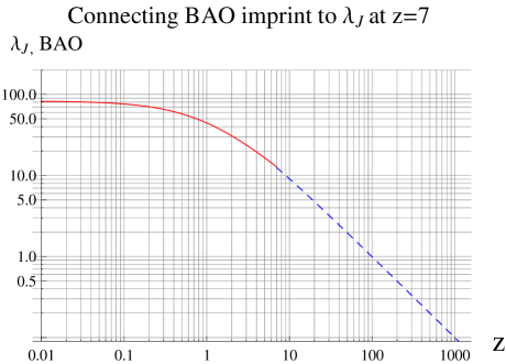
Figure 1: Solid: the Jeans length $\lambda_{J}(t)\propto a^{0.9}$ for $\eta=\frac{3}{5}$; Dashed: the comoving BAO imprint. They are connected at $z=7$, ie, the imprint is transferred to $\lambda_{J}$ at $z=7$ as the initial condition.

An initial rate is also needed to solve (3). Define the rate $r_{a}$ by

$$\frac{\partial}{\partial a}P_{k}(a)=r_{a}P_{k}(a).$$ (19)

The conservation of pair (A.35) at linear level gives

$$r_{a}(z)=\frac{f(\Omega_{m},z)}{a}=(1+z)\,f(\Omega_{m},z),$$ (20)

where $f(\Omega_{m},z)$ is given by Eq.(A.29). From this, we get an estimate of the initial rate $r_{a}\simeq 7$ at $z=7$. As it turns out, the outcomes $\xi$ and $P_{k}$ are actually not sensitive to the value of $r_{a}$ within two orders of magnitude.

The parameters appearing in Eq.(3) are given in the following. The cosmological parameters are taken in the range $\Omega_{m}=(0.25\sim 0.30)$, and $H_{0}^{-1}=3000\,h^{-1}$ Mpc with $h=(0.69\sim 0.73)$ as default, and the outcome correlation function does not change much within the range. To fit with the observed correlation function of galaxies, and of quasars, from surveys [4, 7], we take the three parameters of fluid in the following range

$$k_{J} =(0.045\sim 0.088)\,h\,\mathrm{Mpc}^{-1},~{}~{}i.e.,~{}\lambda_{J}=(139\sim 71)\,h^{-1}\text{Mpc}$$ (21)

$$A =(2\sim 5)\times 10^{3}\,h^{-2}\mathrm{Mpc}^{3},$$ (22)

$$\gamma =1\sim 6.$$ (23)

By (14), $k_{J}$ and $k_{0}$ should be related as follows

$$k_{0} \simeq a^{-\frac{3}{2}+\eta}k_{J}=(1+z)^{\frac{3}{2}-\eta}k_{J},$$ (24)

which is taken only approximately in our computation. The range (21) of $k_{J}$ approximately corresponds to the range (17) of $k_{0}$. From these parameters the sound speed is inferred

$$c_{s0}=(\frac{3}{2}\,\Omega_{m})^{1/2}\frac{H_{0}}{k_{J}}=(2.3\sim 4.5)\times 10^{-3}c\sim(0.6\sim 1.2)\times 10^{3}(\frac{km}{s}),$$ (25)

which is slightly higher than the observed peculiar velocity of galaxies [27]. The particle mass is inferred as

$$m=\frac{H_{0}^{2}A}{4\pi G}\sim 10^{14}M_{\bigodot},~{}~{}\text{for $A=1000$Mpc${}^{3}$}$$ (26)

which is larger than a typical galaxy mass $10^{12}M_{\bigodot}$, and comparable to that of a cluster. The inferred $m$ is expected to be reduced when the nonlinear terms of Eq.(2) that will enhance clustering substantially at small scales are included.

5 The linear solution and its comparison with observations

Given the initial conditions and parameters, by solving Eq. (3) for each $k$ from $z=7$ to $z=0$, we obtain $P_{k}(z)$ as a function of $(k,z)$, and by Fourier transformation we also obtain $\xi(r,z)$ as a function of $(r,z)$. They are plotted in Fig. 2 - Fig. 5, for the sound speed model $c_{s}=c_{s0}a^{-3/5}$. The model $c_{s}=c_{s0}a^{-1}$ has an analogous outcome, its two-surface graphs are not shown to save room.

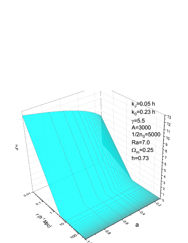
Figure 2: The evolution of correlation function $\xi(r,a)$ from $a=1/8$ to $a=1$ in the model $c_{s}=c_{s0}a^{-3/5}$.

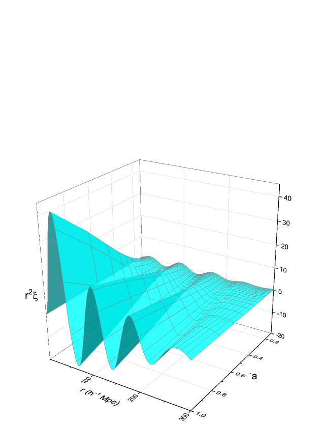
Figure 3: Same as Fig.2. The weighted $r^{2}\xi(r,a)$ exhibits the periodic bumps.

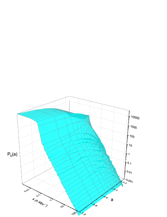
Figure 4: Same as Fig.2. The evolution of power spectrum $P_{k}(a)$. The main peak is at $k\lesssim k_{J}$, and the multi wiggles are developing on the main slope at $k>k_{J}$.

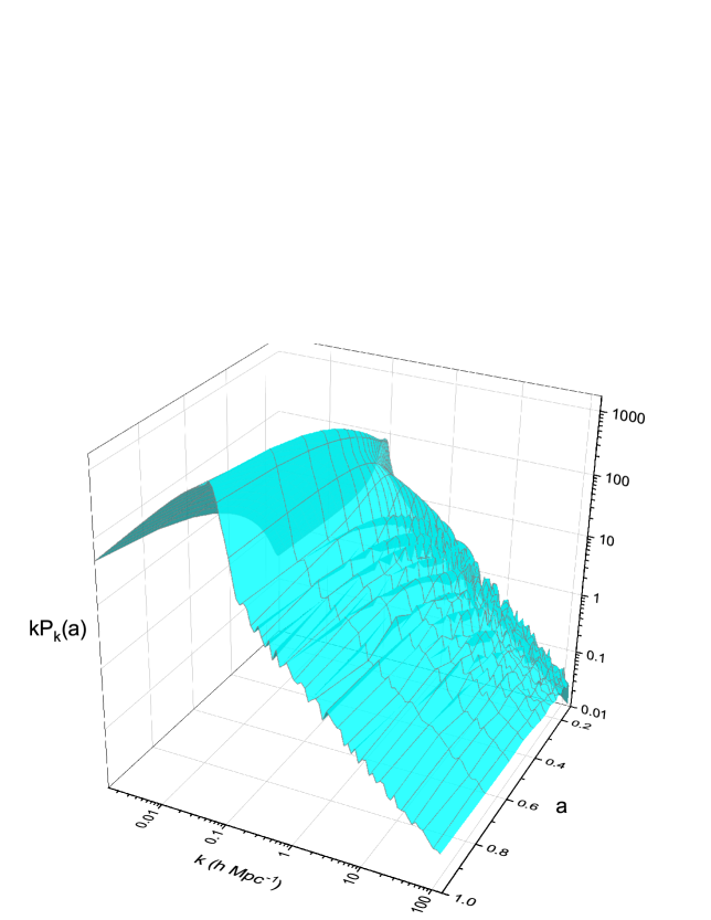
Figure 5: Same as Fig.4. The weighted $kP_{k}(a)$ exhibits the main peak at $k\sim k_{J}$.

During evolution from $z=(7\sim 0)$, the profile of $P_{k}(z)$ keeps a shape similar to the initial power spectrum, increasing in amplitude and developing small wiggles. For $\xi(r,z)$, the separation between periodic bump feature is stretching to a greater distance; the bumps are getting higher and the troughs are getting lower. The solution demonstrates that during $z=(7\sim 0)$ the correlation function at large scales keeps a similar pattern and there is no abrupt change. In this sense we may say that in the expanding Universe the distribution of galaxies is in an asymptotically relaxed state [12].

We compare the solution $\xi(r)$ with the latest observed correlation of WiggleZ galaxies [4] in Fig. 6 for the model $c_{s}=c_{s0}/a^{3/5}$, and in Fig. 7 for the model $c_{s}=c_{s0}/a$.

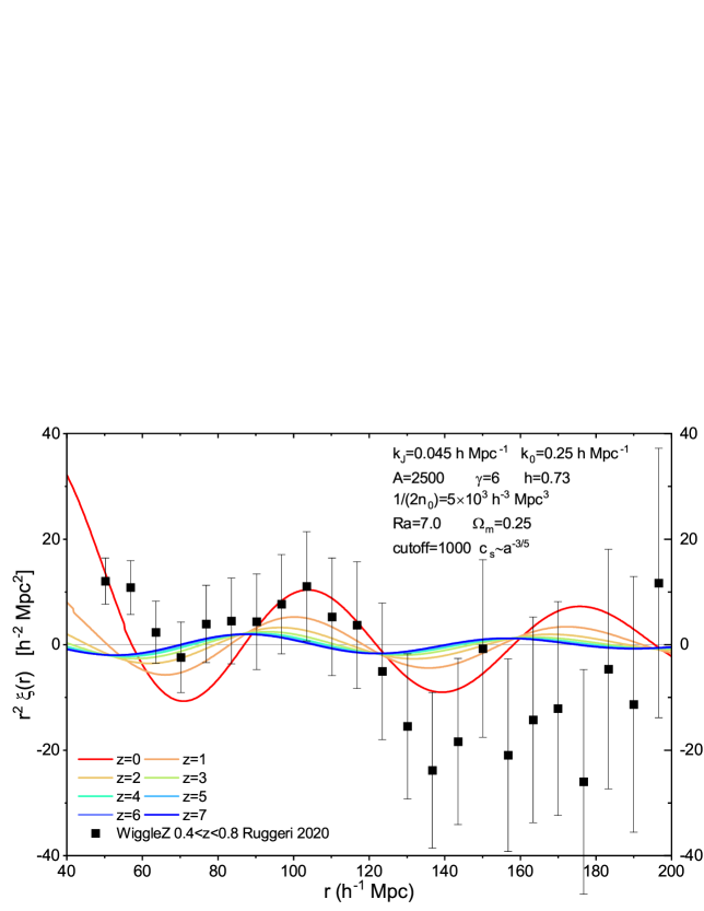
Figure 6: $r^{2}\xi$ of the model $c_{s}=c_{s0}/a^{3/5}$ compared with the data of WiggleZ galaxies in Ref. [4]. The evolution from $z=7$ to $z=0$ are also shown.

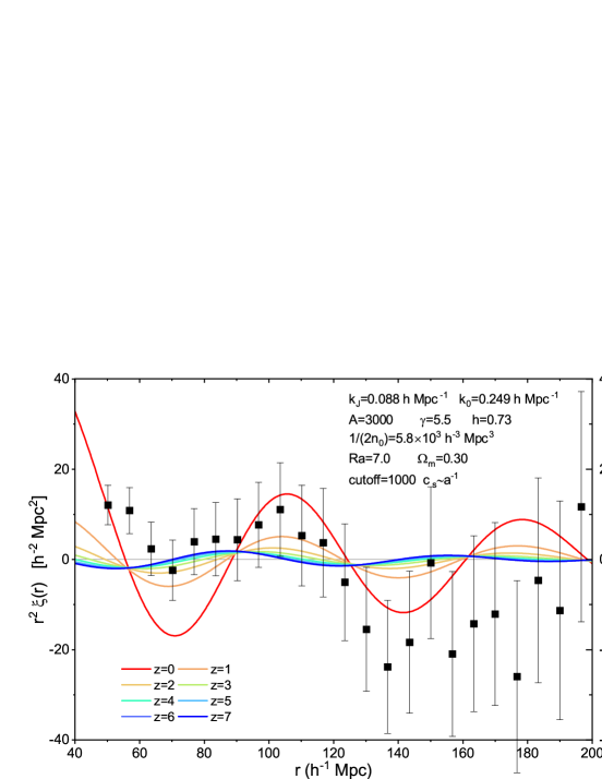
Figure 7: $r^{2}\xi$ of the model $c_{s}=c_{s0}/a$ compared with the data of WiggleZ galaxies in Ref. [4].

We also compare the solution with the observed NGC and SGC quasar data (Ref. [7]) in Fig. 8 and Fig. 9 for model $c_{s}=c_{s0}/a^{3/5}$, and in Fig. 10 and Fig. 11 for the model $c_{s}=c_{s0}/a$. It is seen that the weighted correlation function $r^{2}\xi(r)$ possesses periodic oscillatory bumps along the distance $r$; the height of bumps and the separation between bumps are close to the observed ones. Generally the galaxy and quasar surveys cover regions with different physical environments, so we may choose different values of the parameters within the range listed in Eqs. (21)-(23).

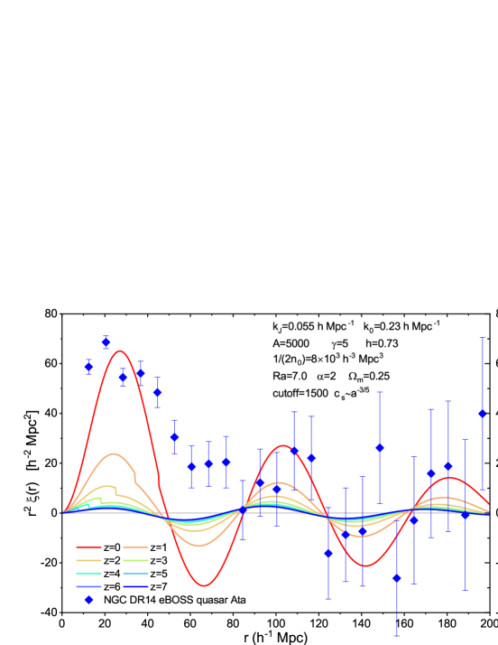
Figure 8: $r^{2}\xi$ of the model $c_{s}=c_{s0}/a^{3/5}$ compared with the data of NGC quasars in Ref.[7].

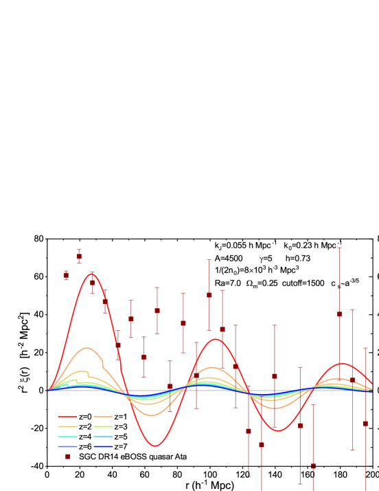
Figure 9: $r^{2}\xi$ of the model $c_{s}=c_{s0}/a^{3/5}$ compared with the data of SGC quasars in Ref.[7].

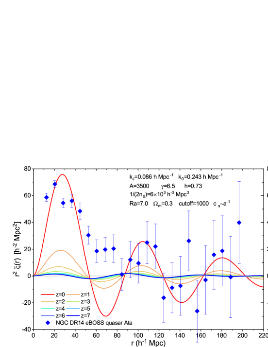
Figure 10: $r^{2}\xi$ of the model $c_{s}=c_{s0}/a$ compared with the data of NGC quasars in Ref. [7].

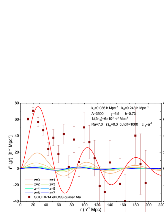
Figure 11: $r^{2}\xi$ of the model $c_{s}=c_{s0}/a$ compared with the data of SGC quasars in Ref. [7].

Equation (8) can also apply to the correlation function of clusters when the appropriate parameters $m$ and $c_{s0}$ are used for the system of clusters. The mathematical structure of Eq. (8) remains the same for galaxies and for clusters, except that clusters have a higher source amplitude $A\propto m$. This explains why the observed correlation functions of clusters have a similar profile to that of galaxies, but with a higher amplitude at small scales. These properties were previously predicted in the static case [14, 15], and also hold in the expanding Universe.

The amplitudes of $\xi$ and $P_{k}$ are increasing during evolution $z=(7\sim 0)$, as seen in Fig. 12 and Fig. 13 for the model $c_{s}=c_{s0}a^{-1}$. The growth varies with different scales. For instance, roughly $\xi(a)$, $P_{k}(a)\propto a^{0.2}$ at small scales ($\xi$ at $r=1h^{-1}$ Mpc, $P_{k}$ at $k=1h$ Mpc^-1), and $P_{k}(a)\propto a^{1.4}$ at large scales ($k=0.05h$ Mpc^-1).

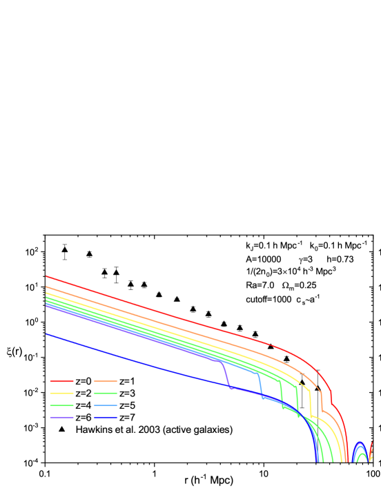
Figure 12: The model $c_{s}=c_{s0}/a$. The growing $\xi(r)$ from $z=7$ to $z=0$. The observational data (triangle) is from Ref. [38].

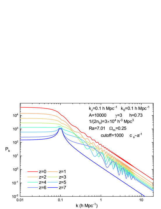
Figure 13: Same as Fig. 12. The growing power spectrum $P_{k}$ from $z=7$ to $z=0$.

The profile of the linear solution $\xi(r)$ has a global maximum with a power-law slope, $\xi\propto r^{-1}$ at $r\lesssim 10$Mpc, which is referred to as the main mountain in this paper. The slope is flatter than the observed [$\xi=(r/r_{0})^{-1.7}$] [39, 40, 41], and will not be improved by merely increasing the mass $m$. This reflects the limitation of the linear solution at small scales. We expect the mountain will get higher and steeper by nonlinear terms, as has been shown in the static nonlinear solution [15]. At high $k>k_{J}$, the profile of spectrum $P_{k}\propto k^{-2}$, the same as that of the initial power spectrum (16). This is referred to as the main slope of $P_{k}$ and corresponds to the main mountain of $\xi$. Note that the linear spectrum $P_{k}$ at high $k$ will lead to a divergent autocorrelation $\xi(0)$ in (11) at the upper limit $k=\infty$ of integration. This UV divergent behavior is analogous to an inflaton scalar field in the inflationary Universe, and can be removed by adiabatic regularization to an appropriate order [42, 43]. If the nonlinear terms are included, the behavior of $P_{k}$ at high $k$ is expected to be modified, deviating from the linear one.

6 The bumps and the wiggles

We analyze the prominent features, i.e., the bumps in $\xi$ and the wiggles in $P_{k}$, in the following.

(1) The most prominent features are the periodic bumps in the correlation function. At large distance, $\xi$ consists of the periodic bumps which are approximately located at

$$r\sim 100,\,180,\,270\,\text{Mpc},...,$$ (27)

with the separation between two neighboring bumps is approximately

$$\Delta r\sim(80\sim 100)\,\text{Mpc}.$$ (28)

The bumps are more clearly seen in the weighted correlation $r^{2}\xi(r)$ plotted in Fig. 3, Figs.6-11. The data from surveys of galaxies [4] and of quasars [7] exhibit the first bump at 100 Mpc, and the negative trough on the interval ($130\sim 160$)Mpc, as well as indicate the existence of a second bump at $\sim 200$Mpc. This agrees with the prediction (27). The 100Mpc periodic bumps were predicted in the static solution [14, 15], and now also show up in the evolution solution in the expanding Unverse. The bump locations (27) and the separation $\Delta r$ (28) are largely determined by $\lambda_{J}$, but also affected by the overdensity $\gamma$, the sound-speed model, the cosmic expansion, and the details of the initial spectrum as well, as we shall analyze in Sect 7.

Early pencil-beam redshift surveys already showed the 100 Mpc periodic feature in the correlation function of galaxies [44, 45, 46] and of clusters [47, 48, 49, 50, 51]. Recent surveys have already shown the existence of two bumps, one at $\sim 100$Mpc and another at $\sim 200$ Mpc, in the correlation function of galaxy [4, 1, 3, 52, 6, 2], as well as of quasars [7, 9, 8, 5, 53]. All these observational results confirm the prediction of a periodic feature (27). Some simulations also show this phenomenon [54, 55]. Large surveys in the future might have a chance of detecting the third bump at $\sim 300$ Mpc in (27).

The 100 Mpc periodic bump feature follows from Eq.(8) by a qualitative analysis. For simplicity, we let $a=1$ and neglect the subdominant expansion term $2H\dot{\xi}$ as approximation, then Eq.(8) reduces to

$$\ddot{\xi}-c_{s0}^{2}\nabla^{2}\xi-4\pi G\rho_{0}\xi=4\pi Gm\delta^{(3)}({\bf r}).$$

Using a time-frequency Fourier transformation $\xi({\bf r},t)=\frac{1}{2\pi}\int d\omega\,\xi_{\omega}({\bf r},\omega)e^{-i\omega t}$, we can solve a Helmholtz equation for each frequency mode $\xi_{\omega}$, and get

$$\xi(r,t)\sim\sum_{\omega}b_{\omega}\frac{Gm}{r}\cos\Big{[}(k_{J}^{2}+\frac{\omega^{2}}{c_{s0}^{2}})^{1/2}r\Big{]}e^{-i\omega t}.$$ (29)

The lowest-frequency mode in (29) reduces to the static solution [56, 14]

$$\xi\sim b_{0}\frac{Gm\cos(k_{J}\,r)}{r},$$ (30)

where $\cos(k_{J}\,r)$ gives rise to the periodic bumps with the separation being the Jeans length $\lambda_{J}=2\pi/k_{J}$. Besides, there are other modes in (29), oscillating at various higher frequencies, referred to as the sub-bumps, whose wavelengths are roughly a fraction of the Jeans length,

$$\lambda\simeq\frac{\lambda_{J}}{l},~{}~{}l=2,3,4,...,$$ (31)

and their amplitudes are much lower than that of the bumps, by orders of magnitude, and thus are barely noticeable in the graphs. The current observational data are insufficient to exhibit these sub-bumps either. These sub-bumps are associated with the wiggles in $P_{k}$, as we shall analyze later.

Since its discovery in 1990s the $100$ Mpc periodic bump feature has been interpreted by various tentative models [44, 45, 46, 47, 48, 49, 50, 51]. More recently it was interpreted as being caused by the imprint of the sound horizon [57]. In the following we analyze the issue of sound horizon and clarify certain statistical concepts involved. The sound horizon was defined as an integration from $z=\infty$ to the decoupling epoch [36, 37]

$$s =\int_{0}^{t(z_{d})}\frac{c_{s}}{a(t)}\,dt=\int_{0}^{t(z_{d})}c_{s}\,(1+z)\,dt,$$ (32)

where the sound speed of baryon gas is [29, 30, 36, 37]

$$c_{s}=\frac{1}{\sqrt{3(1+R)}},~{}~{}~{}R=\frac{3\rho_{b}}{4\rho_{\gamma}}\simeq 31.5\Omega_{b}\,h^{2}(\frac{1000}{z}).$$ (33)

For $\Omega_{m}=0.30$, $\Omega_{b}=0.045$, and $h=0.70$ as the default in this analysis, the decoupling is $z_{d}\simeq 1020$, the integration (32) gives

$$s \simeq 167\,\text{Mpc}.$$ (34)

For $a=1/(1+z)$, the value (34) is also the the present proper length [58]. The sound horizon (32) is sometimes interpreted as the comoving distance that baryon acoustic sound waves travel. With the observations of correlation function of galaxies, the value (34) is not comparable to the observed $100$ Mpc feature, instead, higher by about 60%. Moreover, the sound horizon as a distance ruler can not give a simple explanation of the negative trough at ($130\sim 160$)Mpc, nor the second bump at $\sim 200$Mpc. (See Figs. 6-12.) Therefore, the conventional interpretation of the observed features in terms of the distance traveled by the BAO waves is in doubt and needs to be reexamined. In Ref. [36] on CMB anisotropies and BAO, the sound horizon (32) together with $k$, occurs as the phase $\int\omega d\tau=\int kc_{s}d\tau=ks$ of $k$-modes of BAO, but not as a distance that waves travel. Waves of small density perturbations in the baryons and photons around the decoupling can be described by a homogeneous-Gaussian stochastic process on the three-dimensional space [59, 60, 61]. The important point is that the path of the wave is unobservable statistically, as is the distance of the path. For instance, in Ref.[62], the plot of the potential $\phi_{r}(r,t)$ of the baryon-photon density perturbation in position space is given, for illustration purpose, with a fixed normalized amplitude and a fixed initial point. But the actual situation is not deterministic and $\phi_{r}(r,t)$ is, in fact, a Gaussian random field on three-dimensional space. At a fixed time, the potential $\phi_{r}(r_{i},t)$ is a Gaussian random variable at each point $r_{i}$, and its $n$-point probability distribution is a multivariate Gaussian, schematically written as [59] $P(r_{1},...,r_{n})=[(2\pi)^{n}\,\text{det}(\chi(r)))]^{-1/2}\exp{\big{(}-\frac{1}{2}\sum_{i=1}^{n}\frac{\phi_{r}^{2}(r_{i})}{\chi(r_{i})}\big{)}}$, where $n$ is an arbitrary integer, and $\chi(r)$ is the covariance (the correlation function) of the random variable $\phi_{r}(r_{i})$. When we want to identify a point $r_{i}$ of the possible path of the wave according to its amplitude $\phi_{r}(r_{i})$, the observed amplitude at the point $r_{i}$ may be not what we expect since it is a random variable, thus we do not know if the point $r_{i}$ belongs to the path or not. Thus, we are not able to observe the path of the wave, nor the distance of the path. Equivalently, the potential $\phi_{r}$ can be described in $k$-space as a sum of infinitely many modes [59], $\phi_{r}(r,t)=2\sum_{\bf k}\phi_{r}(k,t)\cos({\bf k\cdot r}+\theta_{k})$, where each mode $\phi_{r}(k,t)$ is a wave traveling along the $\bf k$ direction with a random phase $\theta_{k}$ equally distributed on $[0,2\pi]$. At a fixed time, $\phi_{r}(k,t)$ is a random variable prescribed by a Gaussian probability distribution, $P(\phi_{r}(k))=\exp{\big{(}-\frac{1}{2}\phi_{r}^{2}(k)/p_{k}\big{)}}$, where $p_{k}$ is the power spectrum. When we want to identify a wave of wave number $k$ according to its amplitude $\phi_{r}(k)$, the observed amplitude may be not what we expect, thus we do not know if the observed wave is the one we are seeking. Moreover, generally we see a number of waves with wave numbers close to $k$, and we can not distinguish them, due to a limited precision of measurement of $k$. When we have to pick up one of them arbitrarily, we will face another problem. These waves with different random phases may have traveled different distances. Eventually we do not know the distance the wave has traveled. From the above discussion we conclude that, in both position space and $k$-space for a Gaussian random field, the traveled paths of waves are wiped out statistically, and the traveled distance is unobservable, as is the sound horizon as a traveled distance in the baryon plasma. (In contrast to the Gaussian random process, when a piece of stone is dropped in a calm pond, we are able to observe the path of the wave in perturbed water, and to measure the traveled distance. This is, nevertheless, a deterministic case, unlike the baryon acoustic waves at the decoupling.) The situation of BAO at decoupling is like an instant snapshot of the sea surface full of random waves, unlike the calm pond perturbed by a piece of stone. What we can extract from this photo of ocean surface is the characteristic wavelengths of ocean waves, i.e., the power spectrum of ocean waves, but not the path of waves from an earlier instant. Just as Sunyaev and Zel’dovich [29] correctly pointed out, “note that only observations of the small-scale fluctuations of relic radiation with a periodic dependence on scale may give information on the large-scale density perturbations.”

The sound horizon appears in the spectrum of BAO that contains several characteristic peaks [29, 30, 35, 36], and the separation between these peaks is approximately equal to half of the sound horizon (32) [62]. In this regard, the sound horizon encoded in the spectrum is an observable, but not as a distance traveled by BAO random waves. In our model, the initial power spectrum (16) of the system of galaxies includes one pertinent peak of the BAO spectrum, so the resulting correlation function contains part of the information of BAO spectrum. But the influence of the peak of BAO spectrum is degenerate with the other parameters, such as $\lambda_{J}$, $\gamma$ and the sound speed model. Our computation tells us that, from the solution $\xi$, it is hard to infer the peak of BAO spectrum to a sufficient accuracy.

(2) Another prominent feature are the multiwiggles in the spectrum $P_{k}(z)$, which occur at high $k>k_{J}$, as seen in Fig. 4, Fig. 5, and Fig. 13. Firstly $P_{k}$ has a smooth global maximum plateau, which appears as the sharp peak in the weighted $kP_{k}$ and is located at $k\simeq k_{J}\sim 0.1$Mpc^-1. We refer to it as the main peak. By Fourier transformation, the main peak gives rise to the 100 Mpc periodic bumps in $\xi$. The wiggles show up on the main slope at high $k>k_{J}$. By performing Fourier transformation, the wiggles are not associated with the periodic bumps of $\xi$, but rather associated with the sub-bumps in (31), and are located roughly at

$$k\sim lk_{J},~{}~{}l=2,3,4,...,$$ (35)

and their heights are much lower than the main peak. Both the main peak and the wiggles are already observed in galaxy and quasar surveys [3, 7]. Comparing the observations, the overall profile of the solution $P_{k}$ agrees with the observed data, but contains many wiggles at high $k$, which are expected to be damped considerably when nonlinear terms in Eq. (2) are included.

The wiggles are acoustic oscillations of the fluid with pressure, occurring at large $k$ where gravity is subdominant. This can be also demonstrated analytically from Eq. (12), which, by setting $a=1$ and dropping $2H\dot{\xi}$, becomes approximately the equation of a forced oscillator

$$\frac{d^{2}}{dt^{2}}P_{k}+c^{2}_{s0}(k^{2}-k_{J}^{2})P_{k}=4\pi Gm.$$

For $k>k_{J}$, its solution is

$$P_{k}\sim b\cos(c_{s0}k\,t)+\frac{4\pi Gm}{c^{2}_{s0}k^{2}},$$

where $4\pi Gm/c^{2}_{s0}k^{2}$ determines the main slope at $k>k_{J}$, and $b\cos(c_{s0}k\,t)$ gives the wiggles, and the coefficient $b$ is determined by the initial condition. The wiggles are oscillating with time- more drastically for higher $k$ -as seen in Figs. 4, 5, and 13. The separation between two neighboring wiggles is $\Delta k=\frac{2\pi}{c_{s0}t}$ at a fixed time $t$, and is narrowing down during evolution. Taking into account the evolution effect, one has an estimate $\Delta k\sim 0.1$ Mpc^-1 at $z=0$, which agrees with what we see in the graphs. Moreover, the wiggles are developing during evolution even if the given initial spectrum is smooth without wiggles. The power spectrum of static solution [14, 15] does not contain wiggles because the static equation does not contain the term $\frac{d^{2}}{dt^{2}}P_{k}$. Thus, given the wiggles at $z=0$, one can not infer the precise pattern of wiggles at $z=7$, nor the peak of BAO spectrum, because other factors, such as $\gamma$, the details of initial spectrum, etc, also affect the outcome in a complicated way.

7 The influences by the expansion, the parameters and the initial condition

We now demonstrate how the solution is influenced by the expansion, the sound speed model, the three parameters ($A,k_{J},\gamma$) of the fluid, and two cosmological parameters ($\Omega_{m},h$).

(1) the influence of expansion;

For the linear equation in the static case [14], the bump separation $\Delta r$ is just equal to the Jeans length $\lambda_{J}$. But this will be modified in the expanding Universe. Note that $\Delta r$ in $\xi$ is contributed to by all the growing $k$-modes via the Fourier transformation (11). In Eq. (3), the factor $(\frac{k^{2}}{k_{J}^{2}}-\gamma\,a^{2\eta-1})$ determines that the modes with $k<(\gamma\,a^{2\eta-1})^{1/2}k_{J}$ will grow. So, the effective Jeans wave number is

$$k_{J\,eff}=\frac{\gamma^{1/2}k_{J}}{(1+z)^{\eta-1/2}},$$ (36)

which is affected by the expansion, and also depends on $\gamma$ and $\eta$. Given $\gamma=1$, for both models $\eta=1$ and $\eta=3/5$, one has $k_{J\,eff}=\frac{k_{J}}{(1+z)^{\eta-1/2}}\leqslant k_{J}$, so the growing modes have smaller $k$ than the static case, and after $k$-integration , this leads to a separation $\Delta r$ which is larger than $\lambda_{J}$.

(2) the influence of sound speed model;

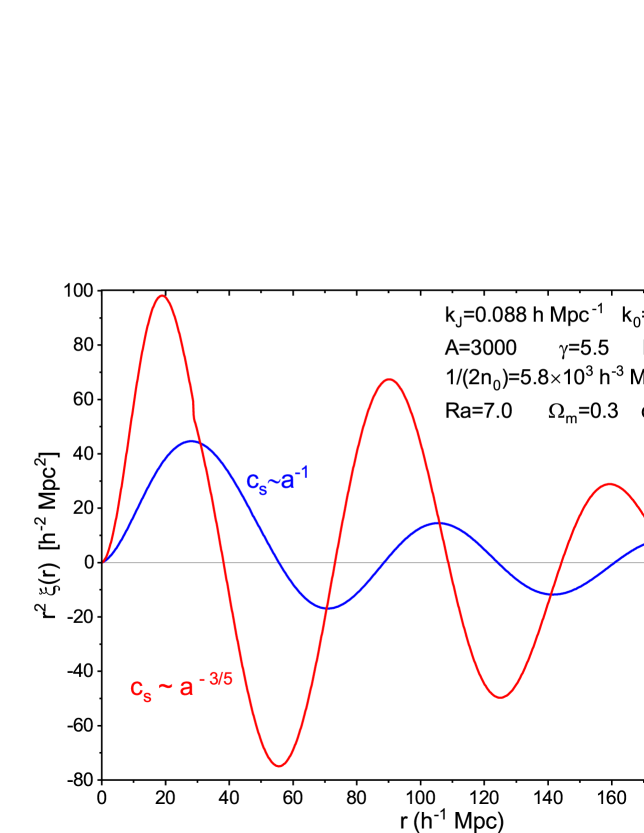
Figure 14: The model $\eta=3/5$ (red line) yields higher bumps and shorter separations than the model $\eta=1$ (blue line). The initial $k_{0}=(1+z)^{1/2}k_{J}$ is taken.

The sound speed models (7) affect the outcome. By $(c_{s0}/a^{3/5})/(c_{s0}/a)=a^{2/5}<1$, the model $\eta=3/5$, comparatively, has a smaller effective sound speed and thus a shorter Jeans length and shorter bump separations. Figure 14 shows $r^{2}\xi$ in the two models. In terms of $P_{k}$, the model $\eta=3/5$ yields a larger effective Jeans wave number, more $k$-modes will fall into the growing modes leading to a higher peak of $P_{k}$ and higher bumps. Besides, the $(k/k_{J})^{2}$ term in Eq. (12) acquires greater effective coefficients, so the wiggles of $P_{k}$ become bigger. By choosing the respective $k_{J}$ appropriately, both models can give $\Delta r$ of (28) that agrees with the observed 100 Mpc feature.

(3) The influence of $k_{J}$;

By the definition of $\lambda_{J}$, a higher density gives a shorter $\lambda_{J}$, and thus yields a smaller separation of bumps. This explains the simulations result [64, 63] that galaxies residing in dense regions have a shorter bump separation. A lower $\lambda_{J}$ also yields a mildly higher clustering amplitude, as seen in Fig.15. This explains the simulation result that galaxies residing in more dense regions give a higher clustering amplitude [64, 63, 65].

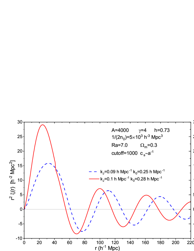
Figure 15: A greater $k_{J}$ leads to a higher mountain at small scales, and shorter bump separations.

(4) The influence of $A$;

The source magnitude $A$ is proportional to $m$. Our computation shows that a larger $m$ gives a higher main mountain at $r\lesssim 50$Mpc, but does not affect the periodic bumps at large distance. In particular, the solution for $A=0$ still contains bumps at large distance. To explain this novel phenomenon, we decompose the solution $\xi$ into two parts

$$\xi=\xi_{1}+\xi_{2},~{}~{}\text{also}~{}~{}P_{k}=P_{k\,1}+P_{k\,2},$$ (37)

where $\xi_{1}$ is the inhomogeneous solution with $A\neq 0$ and the zero initial condition ($P_{k\,ini}=r_{a}=0$), and $\xi_{2}$ is the homogeneous solution with $A=0$ and the nonzero initial condition.

$\xi_{1}$ and $P_{k\,1}$ reflect the influence of $A$, and are shown in Fig.16 and Fig.17. $\xi_{1}$ gives the growing main mountain, but contains no bumps. At any instance of time, $\xi_{1}$ is vanishing beyond the main mountain, so it describes the local clustering around the galaxy with mass $m$. The main mountain is growing radially at the sound speed. $P_{k\,1}$ is flat and smooth without a sharp edge at small $k$, and this explains why here are no bumps in $\xi_{1}$. Moreover, $P_{k\,1}$ is developing multiple wiggles at large $k$ during evolution, even though the initial spectrum is zero. This tells us that the wiggles do not give rise to the periodic bumps in $\xi$.

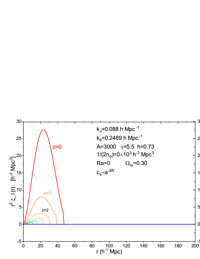
Figure 16: The inhomogeneous $r^{2}\xi_{1}$ generates the main mountain at small $r$ which is growing. There are no bumps at large $r$ beyond the mountain.

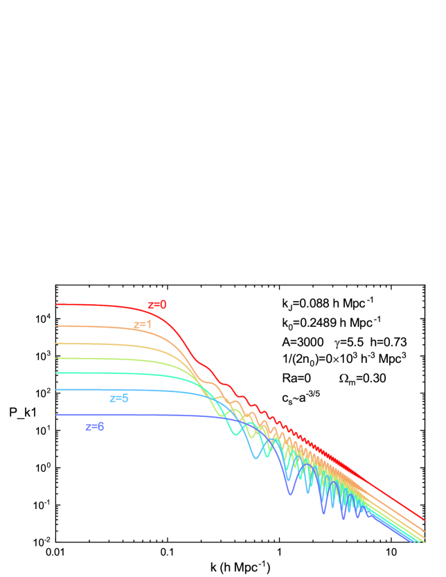
Figure 17: Same as Fig. 16. The inhomogeneous $P_{k\,1}$ has a flat main peak at small $k$ which is shrinking to small $k$ during evolution. Multiple wiggles are developing on the main peak at large $k$.

The homogeneous part $\xi_{2}$ and $P_{k\,2}$ reflect the influence of the nonzero initial condition and are shown in Fig.18, Fig.19, and Fig.20.

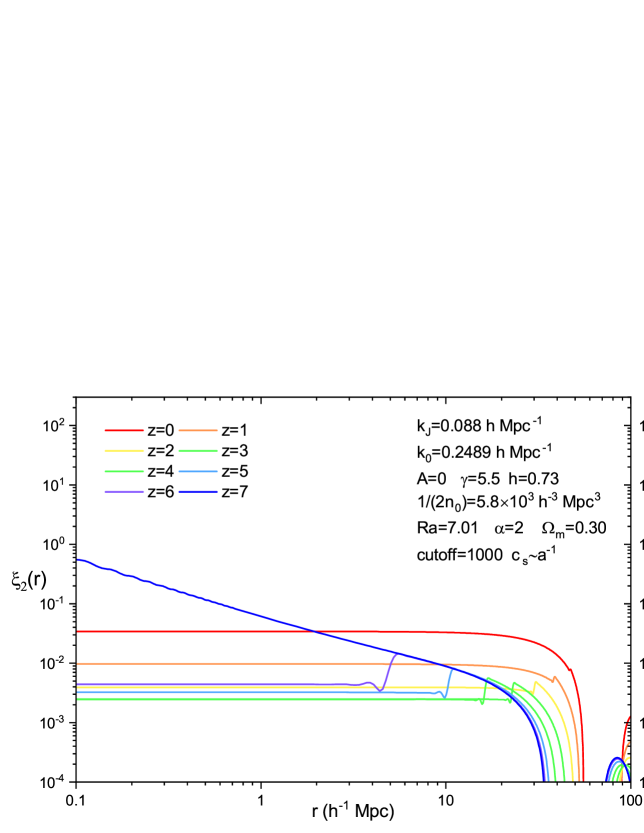
Figure 18: The homogeneous solution $\xi_{2}(r,z)$ forms a plateau on small scales ($r<40\,\mathrm{Mpc}$) at late times ($z\sim 0$).

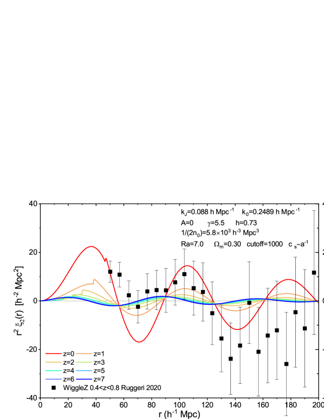
Figure 19: Same as Fig.18. The weighted $r^{2}\xi_{2}(r,z)$ shows the periodic bumps at large scales.

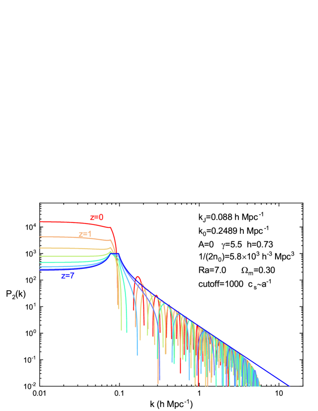
Figure 20: Same as Fig.18. The homogeneous power spectrum $P_{k\,2}(z)$ has a sharp main peak at $k\lesssim k_{J}$, but little power at large $k$.

$\xi_{2}$ contains the periodic bumps at large scales, but forms a flat plateau on small scales $r<40$Mpc at late times. $P_{k\,2}$ has the main peak with a sharp edge at $k\sim k_{J}$ which gives rise to the periodic bumps of $\xi$, but has little power at large $k$, corresponding to the flat plateau in $\xi_{2}$. This reconfirms that the bumps in $\xi$ are associated with the main peak of $P_{k}$, not with the wiggles in $P_{k}$. Moreover, the evolution of $\xi_{2}$ in Fig.19 also shows that the bumps are distributed over the whole $r$ axis, and the bumps are getting higher, the troughs are getting deeper, and the bump separation is getting larger during evolution. This behavior of $\xi_{2}$ for the large scale structure differs from that of $\xi_{1}$ for the local clustering. It should be mentioned that the main mountain of $\xi$ is a superposition of $\xi_{1}$ and the first bump of $\xi_{2}$.

From the decomposition in the above, we conclude that the main mountain of $\xi$ at $r\lesssim 50$ Mpc is due to the source $A$, while the periodic bumps at large distance are seeded by the nonzero initial condition (16). Thereby, at the linear level the small scale clustering and the large scale structure are separated into are two different problems. In Appendix B we also express the decomposed solutions in terms of the Green’s function, and demonstrate the wave nature of correlation function.

(5) The influence of density ratio $\gamma$;

The ratio $\gamma$ defined by Eq. (6) is the fluid density over the cosmic background matter density, and can be regarded as the region overdensity of survey over the background density. A larger $\gamma$ yields higher bumps and deeper troughs, and simultaneously shifts the bump locations of $\xi$ to small distance, as shown in Fig. 21.

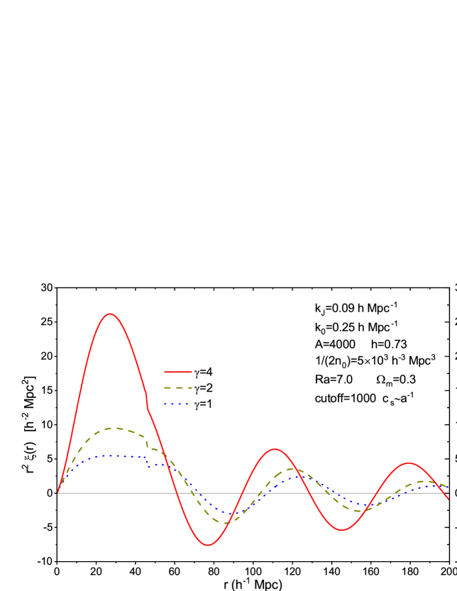
Figure 21: A greater $\gamma$ gives higher bumps and deeper troughs and shifts the bumps to a smaller distance.

(6) The dependence on $\Omega_{m}$;

The matter fraction $\Omega_{m}$ of the cosmic background also affect slightly the correlation and clustering. A high $\Omega_{m}$ enhances slightly the height of the bumps, but does not change the bumps separation, as seen in Fig.22, where $k_{J}$ and $\gamma$ are fixed. $\Omega_{m}$ actually occurs in the definition of $k_{J}$ in Eq. (13). If we would allow $k_{J}$ to vary with $\Omega_{m}$, then a larger $\Omega_{m}$ will correspond to a larger $k_{J}$ and will lead to a shorter bump separation.

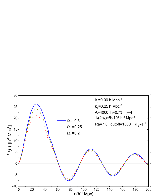
Figure 22: A high $\Omega_{m}$ gives slightly higher bumps at $z=0$, but makes no change in the separation between bumps.

(7) The dependence on $h$;

The Hubble parameter $h$ occurs in the source amplitude $4\pi Gm/H_{0}^{2}$ of Eq. (3) and in the definition of $k_{J}$ in (13). So a small $h$ amounts to a greater $m$ and a greater $k_{J}$.

We now demonstrate the influence of the initial condition (16) and (20). Beside the parameters, the initial power spectrum is another important factor that affects the solution of Eq. (3). To get a smooth solution, the initial condition should be in a range in accordance with the given parameters.

(1) the influence of initial Jeans wave number $k_{0}$;

Our computation shows that it is necessary that the initial spectrum possess certain sharp peak or wedge which is located at $k_{0}$, for the periodic bumps to develop in $\xi$. As mentioned in Sect 4, the initial peak position $k_{0}$ can be viewed as an imprint of the peak of the BAO spectrum, and its value is related to $k_{J}$ through the relation (24) by default. If $k_{0}$ varies slightly from the relation, then a greater $k_{0}$ leads to lower bumps and shorter bump separations in $\xi(r)$, as shown in Fig. 23. We have seen that the influence of $k_{0}$ is degenerate with the parameters $\gamma$ and $\eta$ to various extents, on the outcome $\xi$ and $P_{k}$. As our computation shows, $k_{0}$ should not be allowed to deviate too much, otherwise the evolution may be not sufficiently smooth.

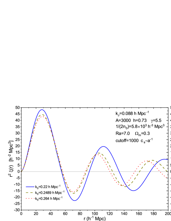
Figure 23: A greater $k_{0}$ leads to lower bumps and shorter bump separations.

(2) the influence of initial amplitude $1/2n_{0}$;

$1/2n_{0}$ is used to represent the amplitude of the initial power spectrum in (16). A higher $1/(2n_{0})$ yields a higher amplitude at $r\lesssim 50$Mpc and a deeper first trough in $\xi$, but leads to a complicated pattern for the subsequent bumps and troughs, as seen in Fig. 24. The main peak of $P_{k}$ is also slightly enhanced but the wedge also shifts to large $k$, and there is little change at large $k\gtrsim 0.2$ Mpc^-1. In the limiting case of a vanishing initial power spectrum, $P_{k\,ini}=0$, the solution is the inhomogeneous $\xi_{1}$ that has no bumps and has been analyzed below Eq. (37) and in Appendix B.

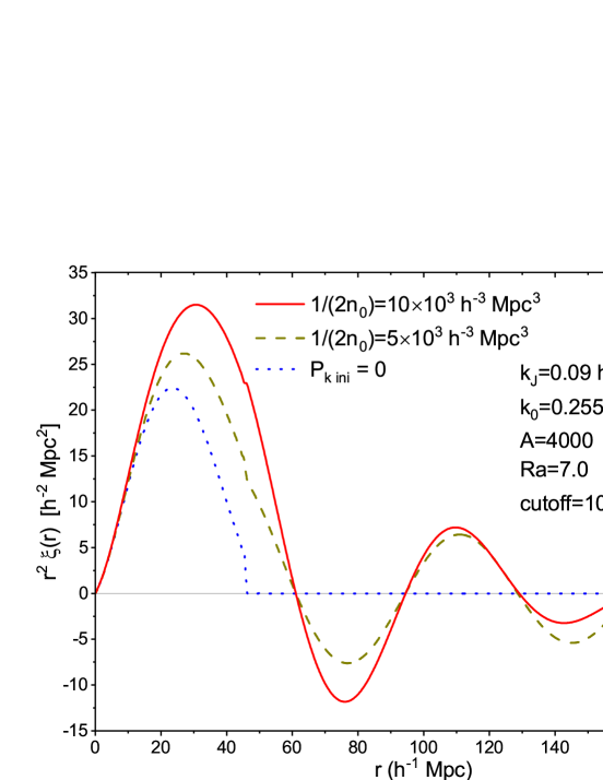
Figure 24: The influence of $1/2n_{0}$ upon $r^{2}\xi$. A higher $1/(2n_{0})$ yields a higher amplitude at $r\lesssim 50$ Mpc. In particular, when the initial power spectrum is vanishing, $P_{k\,ini}=0$, the solution is contributed only by the inhomogeneous $\xi_{1}$. There are no oscillatory bumps in $\xi$ at large $r$, but the main mountain still exists at small scales.

(3) the influence of initial rate $r_{a}$;

The default initial rate is $r_{a}=7.0$ by (20). We find that the evolution pace and outcome are not sensitive to the initial rate $r_{a}$ within two orders of magnitude. This is because in Eq. (3) the coefficient of $\frac{\partial}{\partial a}P_{k}$ is given by $\sim\frac{3}{2a}$, which is about three orders lower than the coefficient of $P_{k}$ term at $z=7$, so that a small variation of $r_{a}$ gives no substantial change to the solution. This also means that the impact of expansion is subdominant to those of pressure and gravity for the system of galaxies during the epoch from $z=7$ to $z=0$.

8 Conclusion and Discussion

Based on the hydrodynamical equations of a Newtonian self-gravity fluid, we derived the nonlinear equation of the correlation function of density perturbation in a flat expanding universe. This extends our previous work in the static universe [14, 15]. Our nonlinear equation is compared with Davis and Peebles’ equation [11] in the following.

Like Davis and Peebles, we use a self-gravity fluid model to describe the system of galaxies in the expanding Universe. Starting from statistical distribution, Davis and Peebles start with the Liouville’s equation and derive a series of BBGKY equations of two-point correlation functions with cutoff. This is a standard method for many-body systems. We describe the system of galaxies by the density $\psi$ which is a stochastic field, apply functional differentiation on the ensemble average of the density field equation (1), perform expansion in terms of density perturbation, and obtain Eq. (2) of two-point correlation function. Our method is commonly used in field theory, and the derivation involves less algebraic calculations. Our Eq. (2) is analogous to Davis and Peebles’ Eq. (47), except there is a factor of two for the gravity term [11]. From the outcome, the BBGKY series is effectively equivalent to the expansion of density perturbations that we have used. We have assumed the generating functional (A.13) for the density field, which is also a prescription of the statistic of the field. The resulting evolution of correlation function is smooth, and the large-scale structure keeps a similar pattern during evolution $z=(7\sim 0)$. In this sense, the system is in an asymptotically relaxed state [12].

There are several differences. To deal with the velocity terms that occur in Eq. (2), we have used the Zel’dovich approximation to replace the velocity by an integration of the density field, and arrived at Eq. (2) which contains three-point and four-point correlation functions. This hierarchy is generally anticipated for a many-body system with interaction and also for a nonlinear field. To deal with three-point and four-point correlation functions, we adopt the Kirkwood-Groth-Peebles ansatz and the Fry-Peebles ansatz, and obtain the main Eq. (2), which is a closed equation for the two-point correlation function as a single unknown function. Davis and Peebles [11], without using the Zel’dovich approximation, derived the differential equations of the velocity and of velocity dispersions, and arrived at a set of five equations (71a), (71b), (72), (76), and (79) for five unknowns. For practical application, one needs to to specify an initial condition which should be consistent for the five unknowns. This would not be easy since one generally lacks sufficient information of these quantities at early epoch. Moreover, the pressure term $c_{s}^{2}\nabla^{2}\xi$ and the $\delta^{(3)}$ source term were ignored in Davis and Peebles’ final equations, so that the acoustic properties (the periodic bumps and wiggles) and the local clustering at small scales (the main mountain) would not appear.

Our Eq. (2) is nonlinear, also integro-differential. In this paper we only solve its linear version, ie, the linear equation (5), apply it to the system of galaxies. For specific computation, we adopt two models of $c_{s}$ in (7). The initial power spectrum (16) at $z=7$ is taken from that of the static solution, and inherits a portion of the imprints of the BAO spectrum that has survived the Silk damping around the decoupling. The initial rate $r_{a}$ is specified by (20) based on the pair conservation.

The linear solution $\xi$ contains a power-law main mountain at small scales and the periodic bumps at large scales. These were previously predicted in the static solution, and confirmed by the observations. Taking advantage of the linearity, we also decompose the solution into homogeneous and inhomogeneous solutions, $\xi=\xi_{1}+\xi_{2}$, and analyze these solutions in terms of Green’s function. $\xi_{1}$ is proportional to $m$, and generates the growing main mountain, and $\xi_{2}$ gives rise to the growing periodic bumps which are unaffected by $m$. Thereby, the local clustering and the large-scale structure are naturally separated as two problems. The bump separation $\Delta r\sim 100$ Mpc is largely determined by the Jeans length $\lambda_{J}$ but also modified by $\gamma$, the sound speed model, and the initial condition.

The corresponding power spectrum $P_{k}$ contains a main peak which is associated with the periodic bumps, as Fourier transformation shows. $P_{k}$ also contains the multiwiggles which are caused by the acoustic oscillations of the system of galaxies. The wiggles are absent in the static solution, and, nevertheless, are developing during evolution even if the initial spectrum has no wiggles. The wiggles do not generate the 100 Mpc periodic bumps, but rather generate the tiny sub-bumps in $\xi$ which are barely visible. In this perspective, $P_{k}$ gives information of acoustic oscillations more than $\xi$ does. Given the pattern of wiggles at present stage, we are not able to accurately infer the wiggle pattern at $z=7$, because other factors also affect the outcome in a complicated way.

The sound horizon, when interpreted as a distance that baryon acoustic waves traveled, is not directly observable from the plasma. This is because the waves form a Gaussian random field, and the paths of waves are wiped out statistically. Indeed, the predicted value of the sound horizon as a distance ruler is higher than the observed 100 Mpc feature, and can not give a simple account of the negative trough at ($130\sim 160$)Mpc, nor the second bump at $\sim 200$ Mpc. Therefore, the conventional picture of the comoving imprint of sound horizon has a difficulty. The sound horizon actually occurs in the phase of BAO modes -one half of sound horizon is approximately equal to the separation between the characteristic peaks of the BAO spectrum. In our present model, the imprint of BAO is transferred to the initial power spectrum of system of galaxies, say, at $z=7$. Subsequently the pertinent quantity is the Jeans wavelength which departures from comoving. The separation between the observed 100 Mpc bumps is attributed to the Jeans length, and is also modified by the parameters $\gamma$ and $c_{s}$, so it is hard to accurately infer the BAO spectrum from the outcome $\xi$ and $P_{k}$ at $z=0$. When future surveys provide more precise measurement of the second bump at $\sim 200$Mpc, or even observe the third bump at $\sim 300$Mpc, it would be possible to infer information of the BAO spectrum. It should be noticed that the measurement of the Hubble constant using the CMB without using the sound horizon [66, 67] has yielded the result $h\sim 0.72$ which is consistent with the local measurements [68, 69, 70], while those, using the sound horizon, lead to an underestimate $h\sim 0.67$ [71, 72], in sharp contrast to the local measurements. Therefore, the conventional use of the sound horizon as a ruler for cosmological distances should be reexamined for BAO and for CMB as well. Given the Hubble tension between the local measurements and the sound-horizon-based CMB+BAO, this scrutiny is necessary.

Another important lesson from the linear solution is that the Jeans length is the correlation scale of the system of galaxies, and is distinguished from the mass scale of a galaxy or cluster. Since the pioneering studies of BAO around the decoupling [29, 30, 31, 32, 33], the Jeans length [29] and the characteristic peaks in the spectrum [30], were often thought to be associated with a Jeans mass enclosed by the associated volume, such as $10^{17}M_{\odot}$ or $10^{5}M_{\odot}$, in hope for an interpretation of the origin of galaxies and clusters. This is a longstanding problem in cosmology and galaxy formation. According to our linear solution, the imprint of BAO at the decoupling evolves into the present Jeans length $\lambda_{J}$ which is roughly equal to the bump separation $\Delta r$, and the mass enclosed in a sphere of radius $\frac{1}{2}\Delta r$ is given by $\frac{\pi}{6}\rho_{c}\Omega_{m}(\Delta r)^{3}\sim 10^{17}M_{\bigodot}$, just comparable to the Jeans mass predicted by Refs.[29, 30, 33, 31, 32]. Obviously, this Jeans mass does not correspond to the mass scale of a galaxy, nor of a cluster. The decomposition (37) of the solution reveals that the mass scale of a galaxy is described by $m$ which is responsible for the local clustering, and that $\lambda_{J}$ occurs not as a (virilized) galactic object, but as the correlation length of galaxies, which is responsible for the large scale structure. The two parameters $\lambda_{J}$ and $m$ reflect two different aspects of the system of galaxies in the Universe. Thereby, one realizes that, in the fitting formula of observed correlation function $\xi=(r/r_{0})^{-1.7}$, the constant $r_{0}$ is really not a correlation length, but a phenomenological parameter which reflects the effects of $m$ and nonlinearity at small scales.

Obviously the linear solution has shortcomings on small scales. The slope of main mountain of $\xi$ is too flat, leading to an overestimated mass $m$ for a galaxy. The predicted wiggles in $P_{k}$ at high $k$ are undamped. These are due to the absence of nonlinear terms from Eq. (8), which are dominant at small scales. In future, we shall study the nonlinear effects.

Appendix A Derivation of the nonlinear equation of correlation function

We first list the field equation of mass density which is the basis for the equation of correlation of density perturbations. The system of galaxies is described by a Newtonian self-gravity fluid, whose hydrodynamical equations consist of the following [73, 17]

$$\frac{\partial\rho}{\partial t}+\nabla_{\bf r}\cdot(\rho{\bf V}) =0,$$ (A.1)

$$\frac{\partial\bf V}{\partial t}+({\bf V}\cdot\nabla_{\bf r}){\bf V} =-\frac{1}{\rho}\nabla_{\bf r}p-\nabla_{\bf r}\Phi,$$ (A.2)

$$\nabla^{2}_{\bf r}\Phi =4\pi G\rho-\Lambda,$$ (A.3)

where $\bf r$ is the proper distance from some chosen origin, $\bf V$ is the proper velocity, and $\Phi$ is the gravitational potential. The pressure $p$ is comparatively small and its contribution to the potential is neglected, but the pressure gradient is included in the Euler equation to show the acoustic behavior of the fluid. These equations are valid for a static universe within the framework of Newtonian gravity. To pass to the expanding Universe, we write $\bf r$ as ${\bf{r}}=a(t)\bf x$ where $\bf x$ is the comoving coordinate. (We choose $a=1/(1+z)$, so that ${\bf r}={\bf x}$ at $z=0$.) Then one has the following

$$\nabla_{\bf r}=\frac{1}{a}\nabla_{\bf x},\ \ \ \ \left(\frac{\partial}{\partial t}\right)_{\bf r}=\left(\frac{\partial}{\partial t}\right)_{\bf x}-\bf{V_{0}}\cdot\nabla_{\bf r},$$

$${\bf V}=\dot{\bf r}={\bf V_{0}}+{\bf v},$$

where ${\bf v}\equiv a\dot{\bf x}$ is the peculiar velocity field, and ${\bf V_{0}}=H\bf r$ is the Hubble flow velocity. We introduce a new potential

$$\phi\equiv\Phi+\frac{1}{2}a\ddot{a}x^{2}.$$ (A.4)

Then, Eqs.(A.1), (A.2), and (A.3) become [17]

$$\frac{\partial\rho}{\partial t}+3\rho H+\frac{1}{a}\nabla_{\bf x}\,\rho\cdot{\bf v}+\frac{1}{a}\rho(\nabla_{\bf x}\cdot{\bf v})=0\,,$$ (A.5)

$$\frac{\partial{\bf v}}{\partial t}+H{\bf v}+\frac{1}{a}({\bf v}\cdot\nabla_{\bf x}){\bf v}=-\frac{1}{a\rho}\nabla_{\bf x}p-\frac{1}{a}\nabla_{\bf x}\phi\,,$$ (A.6)

$$\nabla^{2}_{\bf x}\phi=4\pi Ga^{2}\big{(}\rho-\rho_{0}(t)\big{)}\,,$$ (A.7)

where $\rho_{0}(t)$ is the mean mass density of the fluid, and $\phi$ is contributed only by the matter density fluctuation. We denote $\nabla\equiv\nabla_{\bf x}$. From (A.5), (A.6), and (A.7), one obtains the nonlinear field equation of mass density

$$\ddot{\rho}+8H\dot{\rho}+(15H^{2}+3\dot{H})\rho=\frac{1}{a^{2}}\nabla^{2}p+\frac{1}{a^{2}}\nabla\cdot(\rho\nabla\phi)+\frac{1}{a^{2}}\frac{\partial^{2}}{\partial x^{\beta}\partial x^{\alpha}}({\rho v^{\alpha}}v^{\beta}),$$ (A.8)

which holds a flat expanding universe. Notice that Eq. (A.8) has been derived without using the Friedmann equations explicitly, and the fluid mass density $\rho$ in Eq.(A.8) can be generally higher than the background density of the expanding Universe. Introducing the dimensionless mass density $\psi$ as the following

$$\rho(t,{\bf x})\equiv\rho_{0}(t)\psi(t,{\bf x}),$$ (A.9)

then Eq. (A.8) is written as Eq. (1). Defining the density contrast $\delta$ as

$$\delta({\bf x},t)=\psi({\bf x},t)-1,$$ (A.10)

Eq.(A.8) can be also expressed

$$\frac{\partial^{2}\delta}{\partial t^{2}}+2H\frac{\partial\delta}{\partial t}=\frac{1}{a^{2}\rho_{0}}\nabla^{2}p+4\pi G\rho_{0}(\delta^{2}+\delta)+\frac{1}{a^{2}}\nabla\delta\cdot\nabla\phi+\frac{1}{a^{2}}\frac{\partial^{2}}{\partial x^{\beta}\partial x^{\alpha}}\big{(}(1+\delta)v^{\alpha}v^{\beta}\big{)},$$ (A.11)

which is Eq. (9.19) in Ref. [17]. When the three nonlinear terms are neglected, (A.11) reduces to

$$\frac{\partial^{2}\delta}{\partial t^{2}}+2H\frac{\partial\delta}{\partial t}-\frac{1}{a^{2}\rho_{0}}\nabla^{2}p-4\pi G\rho_{0}\delta=0,$$ (A.12)

which is the Jeans linear equation in the expanding Universe.

The field equation of the two-point correlation function in the expanding Universe can be derived by the functional derivative method, in a similar procedure to the static case [14, 15]. The method is commonly used to get the equation of the two-point correlation function in field theory, such as particle physics and condensed matter [74, 19, 75]. The system of galaxies in the expanding Universe is not too far from equilibrium. The cosmic expansion time scale $t_{e}=\frac{1}{H_{0}}=\sqrt{3/8\pi G\rho_{0}}$, the dynamic time for galaxies moving in the background $t_{d}=\sqrt{3/16\pi G\rho_{0}}$ [23], and the two time scales are of the same order of magnitude. So the system of galaxies is said to be in an asymptotically relaxed state [12]. In statistical mechanics, given the Hamiltonian of a self-gravitating many-body system, the grand partition function is commonly constructed with the temperature $T$ [12]. By the Hubbard-Stratonovich transformation [75], the grand partition function of the discrete many-body system is cast into a path-integral generating functional, either for the gravitational potential field [13], or for the density field $\psi$ [14, 15]. The generating functional facilitates the derivation of correlation functions of the field. We assume that, in the expanding Universe, the generating functional of the density field $\psi$ has the following form

$$Z[J] =\int{\cal D}\psi\exp\Big{[}-\beta\int d^{3}x\big{(}{\cal L}(\psi)-a^{3}J\psi\big{)}\Big{]},$$ (A.13)

and the ensemble average of the field $\psi$ is given by

$$\langle\psi\rangle_{J}=\frac{1}{Z[J]}\int{\cal D}\psi\,\psi\exp\Big{[}-\beta\int d^{3}x\big{(}{\cal L}(\psi)-a^{3}J\psi\big{)}\Big{]},$$ (A.14)

where ${\cal L}$ is the effective Lagrangian density whose variation with respect to $\psi$ leads to Eq. (1), $J$ is the external source introduced as an apparatus for functional differentiation, and $\beta\equiv 1/4\pi Gm$ with $m$ being the particle mass. Although $\beta$ formally plays a role of an ”effective” temperature in $Z[J]$ of (A.13), actually it is not the temperature $T$, the latter has been absorbed into the sound speed $c_{s}$. The notation $\beta$ here is different from that in Refs.[14, 15], and $c_{s}^{2}$ is put into ${\cal L}$ here. In the static case the explicit expression of ${\cal L}$ is known [75, 13, 14, 15]. In the expansion case the linear part of ${\cal L}$ is given by

$${\cal L}_{lin}=a^{3}\Big{(}\frac{1}{2}a^{-1}(\dot{\psi})^{2}-\frac{1}{2}a^{-1}(\frac{c_{s}}{a}\nabla\psi)^{2}+4\pi G\rho_{0}a^{-1}(\frac{1}{2}\psi-1)\psi\Big{)},$$

which corresponds to the part of Eq. (1) without the potential and velocity terms. The nonlinear part of ${\cal L}$ gives rise to the potential and velocity terms in (1) and will be more involved, and we do not need its explicit expression in this paper. Generally speaking, knowing the exact expression of ${\cal L}$ in terms of $\psi$ would amount to knowing the exact nonlinear equation and the non-Gaussian statistic of the field $\psi$. In particular, the non-Gaussian statistic can be represented by various correlation functions of $\psi$ to a sufficient order. Therefore, we want to know the equations of these correlation functions which contain both statistical and dynamical information of the field. The prescription (A.13) with (A.14) of the generating functional is sufficient for our purpose to derive the equations of various correlation functions. In the following we derive the equation of two-point correlation function.

Adding the external source $J$ to Eq. (1) and taking the ensemble average, we get

$$\big{\langle}\ddot{\psi}\big{\rangle}_{J}+2H\big{\langle}\dot{\psi}\big{\rangle}_{J}-\frac{c_{s}^{2}}{a^{2}}\big{\langle}\nabla^{2}\psi\big{\rangle}_{J}-4\pi G\rho_{0}\big{\langle}(\psi^{2}-\psi)\big{\rangle}_{J}$$

$$-\frac{1}{a^{2}}\big{\langle}\nabla\psi\cdot\nabla\phi\big{\rangle}_{J}-\frac{1}{a^{2}}\big{\langle}\frac{\partial^{2}}{\partial x^{i}\partial x^{j}}(\psi v^{i}v^{j})\big{\rangle}_{J}-\langle J\rangle_{J}=0.$$ (A.15)

Applying functional derivative $\frac{\delta}{a^{3}\beta\delta J(\textbf{x}^{\prime})}$ to each term in the above equation and then setting $J=0$, we obtain Eq.(2), where the following have been used. The connected two-point correlation function of the field $\psi$ is defined by the ensemble average

$$G^{(2)}\left(\mathbf{x}_{1},\mathbf{x}_{2},t\right) \equiv\left\langle\delta\psi\left(\mathbf{x}_{1},t\right)\delta\psi\left(\mathbf{x}_{2},t\right)\right\rangle$$

$$=\frac{\delta}{(a^{3}\beta)\delta J({\bf x}_{2})}\langle\psi\left(\mathbf{x}_{1},t\right)\rangle_{J}\Big{|}_{J=0}$$

$$=\left.\frac{\delta^{2}}{(a^{3}\beta)^{2}\delta J({\bf x}_{2})\delta J({\bf x}_{1})}\ln Z[J]\right|_{J=0}$$ (A.16)

where $\delta\psi(\bf{x})=\psi(\bf{x})-\langle\psi(\bf{x})\rangle$ is the dimensionless density fluctuation. One has $\langle\delta\psi({\bf r})\rangle=0$, $\langle\psi({\bf x})\rangle|_{J=0}=1$, and $\delta\psi({\bf x})=\delta({\bf x})$. $G^{(2)}$ is dimensionless by the definition, and is assumed to have the following stationary property

$$G^{(2)}\left({\bf x}_{1},{\bf x}_{2},t\right)=G^{(2)}\left({\bf x}_{1}-{\bf x}_{2},t\right)=G^{(2)}(|{\bf x}_{1}-{\bf x}_{2}|,t),$$ (A.17)

which is consistent with the isotropy of the background Universe. The connected $n$-point correlation function is

$$G^{(n)}\left(\mathbf{r}_{1},\ldots,\mathbf{r}_{n}\right) \equiv\left\langle\delta\psi\left(\mathbf{r}_{1}\right)\ldots\delta\psi\left(\mathbf{r}_{n}\right)\right\rangle$$ (A.18)

$$=\left.\frac{\delta^{n}\ln Z[J]}{(a^{3}\beta)^{n}\delta J\left(\mathbf{r}_{1}\right)\ldots\delta J\left(\mathbf{r}_{n}\right)}\right|_{J=0}$$ (A.19)

$$=\left.\frac{\delta^{n-1}\left\langle\psi(\mathbf{r}_{n})\right\rangle_{J}}{(a^{3}\beta)^{n-1}\delta J\left(\mathbf{r}_{1}\right)\ldots\delta J\left(\mathbf{r}_{n-1}\right)}\right|_{J=0},~{}~{}~{}\text{for $n\geq 2$}.$$ (A.20)

Other terms are calculated in the same manner,

$$\frac{\delta}{(a^{3}\beta)\delta J(\bf{x}^{\prime})}\langle\nabla^{2}\psi({\bf x},t)\rangle\Big{|}_{J=0}=\nabla^{2}G^{(2)}(\bf{x}-\bf{x}^{\prime},t),$$

$$\frac{\delta}{(a^{3}\beta)\delta J(\textbf{x}^{\prime})}\langle\dot{\psi}({\bf x},t)\rangle_{J}\Big{|}_{J=0}=\dot{G}^{(2)}({\bf x},{\bf x}^{\prime},t),$$

$$\frac{\delta}{(a^{3}\beta)\delta J(\textbf{x}^{\prime})}\langle\ddot{\psi}({\bf x},t)\rangle_{J}\Big{|}_{J=0}=\ddot{G}^{(2)}({\bf x},{\bf x}^{\prime},t),$$

$$\frac{\delta}{(a^{3}\beta)\delta J(\textbf{x}^{\prime},t)}\langle\psi^{2}({\bf x})\rangle\Big{|}_{J=0} =\frac{\delta}{a^{3}\beta\delta J(\textbf{x}^{\prime})}\big{(}\langle\psi({\bf x})\rangle\langle\psi({\bf x})\rangle+\langle\delta({\bf x})\delta({\bf x})\rangle\big{)}\Big{|}_{J=0}$$

$$=2G^{(2)}(\textbf{x}-\textbf{x}^{\prime},t)+G^{(3)}(\textbf{x},\textbf{x},\textbf{x}^{\prime};t),$$ (A.21)

where $\langle\psi\rangle_{J=0}=1$ is used. The external source term gives

$$\frac{\delta}{(a^{3}\beta)\delta J(\textbf{x}^{\prime})}\langle J({\bf x})\rangle_{J}\Big{|}_{J=0} =\frac{1}{a^{3}\beta}\delta^{(3)}(\bf{x}-\bf{x}^{\prime}).$$ (A.22)

From these, we get

$$\ddot{G}^{(2)}({\bf x}-{\bf x}^{\prime},t)+2H\dot{G}^{(2)}({\bf x}-{\bf x}^{\prime},t)-\frac{c_{s}^{2}}{a^{2}}\nabla^{2}G^{(2)}({\bf x}-{\bf x}^{\prime},t)$$

$$-4\pi G\rho_{0}(t)\left(G^{(2)}(\textbf{x}-\textbf{x}^{\prime},t)+G^{(3)}(\textbf{x},\textbf{x},\textbf{x}^{\prime},t)\right)$$

$$-\frac{1}{a^{2}}\frac{\delta}{(a^{3}\beta)\delta J(\textbf{x}^{\prime})}\langle\nabla\psi(\textbf{x})\cdot\nabla\phi(\textbf{x})\rangle\Big{|}_{J=0}-\frac{1}{a^{2}}\frac{\partial^{2}}{\partial x^{i}\partial x^{j}}\frac{\delta}{(a^{3}\beta)\delta J(\textbf{x}^{\prime})}\langle(\psi(\textbf{x})v^{i}(\textbf{x})v^{j}(\textbf{x}))\rangle\Big{|}_{J=0}$$

$$=\frac{1}{a^{3}\beta}\delta^{(3)}(\bf{x}-\bf{x}^{\prime}).$$ (A.23)

To deal with the potential term $\nabla\psi\cdot\nabla\phi$ in (A), we use the solution of the Poisson equation (A.7)

$$\phi({\bf x},t)=-a^{2}G\rho_{0}(t)\int\frac{\psi({\bf x}^{\prime},t)-1}{|\bf x-x^{\prime}|}d^{3}{\bf x}^{\prime},$$ (A.24)

$$\nabla\phi({\bf x},t)=-a^{2}G\rho_{0}(t)\int\big{(}\psi({\bf x^{\prime}},t)-1\big{)}\nabla\frac{1}{|\bf x-x^{\prime}|}d^{3}{\bf x}^{\prime}\,,$$ (A.25)

where $\nabla\equiv\nabla_{x}$. So we have

$$\nabla\psi\cdot\nabla\phi=-a^{2}G\rho_{0}(t)\int\bigg{(}\psi({\bf x^{\prime}},t)\nabla\psi({\bf x},t)-\nabla\psi({\bf x},t)\bigg{)}\cdot\nabla\frac{1}{|\bf x-x^{\prime}|}d^{3}{\bf x}^{\prime}.$$ (A.26)

Applying functional differentiation on the ensemble average of (A.26), we get

$$-\frac{\delta}{a^{3}\beta\delta J(\textbf{x}^{{}^{\prime}})}\frac{1}{a^{2}}\langle\nabla\psi\cdot\nabla\phi\rangle\Big{|}_{J=0}= 4\pi G\rho_{0}(t)G^{(3)}(\textbf{x},\textbf{x},\textbf{x}^{{}^{\prime}})$$

$$+G\rho_{0}(t)\int\nabla\cdot\Big{(}G^{(3)}(\textbf{x},\textbf{x}^{\prime},\textbf{x}^{{}^{\prime\prime}})\cdot\nabla\frac{1}{|\bf x-x^{\prime\prime}|}\Big{)}d^{3}{\bf x^{\prime\prime}}.$$ (A.27)

Substituting (A) into (A), noting that $4\pi G\rho_{0}G^{(3)}$ in Eq.(A) will cancel the $-4\pi G\rho_{0}G^{(3)}$ term in Eq.(A), we obtain Eq. (2) of two-point correlation function.

The velocity dispersion term $\psi v^{i}v^{j}$ in (2) can be treated as the following. Under the Zel’dovich approximation [17], the peculiar velocity $v^{i}$ can be expressed in terms of the density field $\psi$

$$\mathbf{v}=-\frac{1}{4\pi G\rho_{0}a}\frac{\dot{D}}{D}\nabla\phi=\frac{Hf\left(\Omega_{m}\right)}{4\pi}a\int(\psi({\bf x}^{\prime},t)-1)\nabla\frac{1}{\left|\mathbf{x}^{\prime}-\mathbf{x}\right|}d^{3}x^{\prime}+O(\delta^{2})$$ (A.28)

where

$$f(\Omega_{m},t)\equiv-\frac{d\ln D}{d\ln(1+z)}=\frac{a}{D}\frac{dD}{da},$$ (A.29)

and $D(t)$ is a growing mode of the linear part of equation (A.11) without pressure [17]. For a flat RW spacetime, it can be approximately fitted by the following formula [76],

$$f(\Omega_{m},t)=\Omega^{0.6}+\frac{1}{70}\big{(}1-\frac{1}{2}\Omega(1+\Omega)\big{)},~{}~{}\text{with}~{}~{}\Omega\equiv\Omega_{m}\frac{(1+z)^{3}}{(\Omega_{m}(1+z)^{3}+\Omega_{\Lambda})^{2}}.$$ (A.30)

Substituting (A.28) into the velocity dispersion term of (A), we calculate

$$\frac{\delta}{a^{3}\beta\delta J({\bf x}^{\prime})}\Big{[}\langle\psi({\bf x})\rangle\langle\delta({\bf y})\delta({\bf z})\rangle+\langle\delta({\bf x})\delta({\bf y})\delta({\bf z})\rangle\Big{]}\Big{|}_{J=0}$$

$$=G^{(2)}({\bf x-x^{\prime}})G^{(2)}({\bf y-z})+G^{(3)}({\bf y,z,x^{\prime}})+G^{(4)}({\bf x},{\bf y},{\bf z},{\bf x}^{\prime}),$$ (A.31)

where the definition (A.18) has been used, and get the following

$$\frac{\delta}{a^{3}\beta\delta J({\bf x}^{\prime})}\langle\psi v^{i}v^{j}\rangle\Big{|}_{J=0}=\frac{H^{2}a^{2}f^{2}(\Omega_{m})}{16\pi^{2}}\iint d^{3}y\,d^{3}z\frac{y^{i}-x^{i}}{|{\bf y}-{\bf x}|^{3}}\frac{z^{j}-x^{j}}{|{\bf z}-{\bf x}|^{3}}$$

$$\times\bigg{(}G^{(2)}({\bf x-x^{\prime}},t)G^{(2)}({\bf y-z},t)+G^{(3)}({\bf y,z,x^{\prime}};t)+G^{(4)}({\bf x,y,z,x^{\prime}};t)\bigg{)}.$$ (A.32)

Substituting (A) into Eq.(2) yields the nonlinear equation (2) which contains $G^{(3)}$ and $G^{(4)}$. By comparison, Davies and Peebles [11] did not use the Zel’dovich approximation, so that their Eq.(72) contains the unknown velocity dispersions. The Zel’dovich approximation will cause an error of the order $\delta^{3}$ in $v^{i}v^{j}$, which would bring about extra terms like $G^{(4)}$ and $G^{(2)}G^{(3)}$ in (A). We shall drop these terms. Therefore, (A) is accurate up to a numerical factor of the term $G^{(4)}$.

To make Eq. (2) closed for $G^{(2)}$, we adopt the Kirkwood-Groth-Peebles ansatz on the three-point correlation function [20, 21],

$$G^{(3)}_{123}=Q\big{[}G^{(2)}_{12}G^{(2)}_{23}+G^{(2)}_{23}G^{(2)}_{31}+G^{(2)}_{31}G^{(2)}_{12}\big{]},~{}~{}~{}Q=1.0\pm 0.2,$$ (A.33)

where $G^{(2)}_{12}$ denotes $G^{(2)}(\mathbf{x_{1},x_{2}},t)$ and $G^{(3)}_{123}$ denotes $G^{(3)}(\mathbf{x_{1},x_{2},x_{3}};t)$ for notational simplicity, and $Q$ is a dimensionless constant to be determined by observation. [We remark that the ansatz (A.33) with $Q=1$ holds exactly as a solution of $G^{(3)}_{123}$ in the Gaussian approximation for the static case [15].] For the four-point correlation function, we adopt the Fry-Peebles ansatz [22]

$$G^{(4)}_{1234}= R_{a}\Big{[}G^{(2)}_{12}G^{(2)}_{23}G^{(2)}_{34}+G^{(2)}_{23}G^{(2)}_{34}G^{(2)}_{41}+G^{(2)}_{34}G^{(2)}_{41}G^{(2)}_{12}+G^{(2)}_{41}G^{(2)}_{12}G^{(2)}_{23}$$

$$+G^{(2)}_{13}G^{(2)}_{34}G^{(2)}_{42}+G^{(2)}_{34}G^{(2)}_{42}G^{(2)}_{21}+G^{(2)}_{42}G^{(2)}_{23}G^{(2)}_{31}+G^{(2)}_{21}G^{(2)}_{13}G^{(2)}_{34}$$

$$+G^{(2)}_{14}G^{(2)}_{42}G^{(2)}_{23}+G^{(2)}_{31}G^{(2)}_{14}G^{(2)}_{42}+G^{(2)}_{31}G^{(2)}_{12}G^{(2)}_{24}+G^{(2)}_{23}G^{(2)}_{31}G^{(2)}_{14}\Big{]}$$

$$+ R_{b}\Big{[}G^{(2)}_{12}G^{(2)}_{13}G^{(2)}_{14}+G^{(2)}_{21}G^{(2)}_{23}G^{(2)}_{24}+G^{(2)}_{31}G^{(2)}_{32}G^{(2)}_{34}+G^{(2)}_{41}G^{(2)}_{42}G^{(2)}_{43}\Big{]}.$$ (A.34)

where $G^{(4)}_{1234}$ denotes $G^{(4)}(\mathbf{x_{1},x_{2},x_{3},x_{4}};t)$, $R_{a}$ and $R_{b}$ are two parameters and observations indicate $3R_{a}+R_{b}\simeq 10\pm 2$ {see (19.23) in ref.[27]}. The undetermined numerical factor of $G^{(4)}$ due to the Zel’dovich approximation can be absorbed into the parameters $R_{a}$ and $R_{b}$. Substituting (A.33) and (A) into (2), using the conventional notation $\xi({\bf x},t)=G^{(2)}({\bf x},t)$, we arrive at the nonlinear Eq. (2) in the context.

By similar calculations, taking functional derivative of the ensemble average of the continuity equation (A.5) and using the Zel’dovich approximation (A.28), we obtain the continuity equation in terms of correlation function

$$\frac{\partial}{\partial t}\xi(\textbf{x}-\textbf{x}^{\prime},t)-Hf(\Omega_{m})\xi(\textbf{x}-\textbf{x}^{\prime},t)+\frac{Hf(\Omega_{m})}{4\pi}\int\nabla\cdot\Big{(}G^{(3)}(\textbf{x},\textbf{x}^{{}^{\prime}},\textbf{x}^{{}^{\prime\prime}})\nabla\frac{1}{\lvert{\bf x^{\prime\prime}}-{\bf x}\rvert}\Big{)}d^{3}x^{\prime\prime}=0.$$ (A.35)

This is closed when the Groth-Peebles ansatz (A.33) is used. Equation (A.35) should be compared with the conservation of particle pair {Eq. (41) or Eq. (71b) in Ref.[11]} which still contains the relative velocity of a pair of galaxies. We have made use of (A.35) to give an estimate of the change rate (20) in the context.

Appendix B The linear solution in terms of the Green’s function

Although we have obtained the numerical linear solution $P_{k}$ and $\xi$, it is revealing to analyze the solution by the Green’s function method. To isolate the influences of the source $A$ and the initial conditions, in accordance with (37) we write

$$\xi({\bf x},t)=\frac{w({\bf x},t)}{a(t)}=\frac{1}{a}(w_{1}({\bf x},t)+w_{2}({\bf x},t)),$$ (B.1)

where $w_{1}$ satisfies the following

$$\left\{\begin{split}&\ddot{w}_{1}({\bf x},t)-c^{2}(t)\nabla^{2}w_{1}({\bf x},t)-m^{2}(t)w_{1}({\bf x},t)=\frac{A}{a(t)^{2}}\delta^{(3)}({\bf x})\\ &w_{1}|_{t=t_{i}}=0\\ &\dot{w}_{1}\Big{|}_{t=t_{i}}=0,\\ \end{split}\right.$$ (B.2)

with

$$c^{2}(t) \equiv\frac{c_{s0}^{2}}{a^{2+2\eta}(t)},$$ (B.3)

$$m^{2}(t) \equiv 4\pi G\rho_{c}\Big{[}\frac{2}{3}(-\frac{1}{2}a^{-3}\Omega_{m}+\Omega_{\Lambda})+\frac{\gamma\,\Omega_{m}}{a^{3}(t)}\Big{]},$$ (B.4)

where the Friedmann equation $\frac{\ddot{a}}{a}=\frac{8\pi G\rho_{c}}{3}(-\frac{1}{2}a^{-3}\Omega_{m}+\Omega_{\Lambda})$ has been used. $w_{1}$ is contributed by the source $A$. In (B.1), $w_{2}$ satisfies the following

$$\left\{\begin{split}&\ddot{w}_{2}({\bf x},t)-c^{2}(t)\nabla^{2}w_{2}({\bf x},t)-m^{2}(t)w_{2}({\bf x},t)=0,\\ &w_{2}|_{t=t_{i}}=a(t_{i})\xi({\bf x},t_{i}),\\ &\dot{w}_{2}\big{|}_{t=t_{i}}=a(t_{i})\Big{(}H(t_{i})\xi({\bf x},t_{i})+\dot{\xi}({\bf x},t_{i})\Big{)},\\ \end{split}\right.$$ (B.5)

where the initial time $t_{i}$ corresponds to the redshift $z=7$, and the $\xi({\bf x},t_{i})$ and $\dot{\xi}({\bf x},t_{i})$ are given by the initial spectrum $P_{k\,ini}$ of (16) and the initial rate $r_{a}$ of (20). $w_{2}$ is contributed by the initial condition. Corresponding to (B.1), the power spectrum is also split into two parts

$$P_{k}=\frac{1}{a}\int d^{3}x\,\Big{(}w_{1}({\bf x},t)+w_{2}({\bf x},t)\Big{)}e^{-i{\bf k\cdot x}}=P_{k\,1}+P_{k\,2}.$$ (B.6)

We obtain numerically the solutions $P_{k\,1}$ and $\xi_{1}$ shown in Fig.16 and Fig.17, as well as $P_{k\,2}$ and $\xi_{2}$ in Fig.18, Fig.19, and Fig.20.

We now express these the solutions in terms of the Green’s function. It can be checked that the principle of homogeneity also applies to the inhomogeneous equation (B.2) with the time-dependent coefficients. So, by Duhamel’s principle, Eq. (B.2) of $w_{1}$ reduces to a homogeneous equation with a nonzero initial velocity, the solution is given by

$$w_{1}({\bf x},t) =\int^{t}_{t_{i}}\Big{[}\int\frac{A}{a^{2}(\tau)}\delta^{(3)}({\bf x_{0}})G({\bf x,x_{0}},t)d^{3}x_{0}\Big{]}d\tau$$

$$=\int^{t}_{t_{i}}\frac{A}{a^{2}(\tau)}G({\bf x},t)d\tau,$$ (B.7)

where $G({\bf x,x_{0}},t)$ is the Green’s function satisfying the following

$$\left\{\begin{split}&\ddot{G}({\bf x,x_{0}},t)-c^{2}(t)\nabla^{2}u({\bf x,x_{0}},t)-m^{2}(t)G({\bf x,x_{0}},t)=0~{}~{}~{}(t>t_{i})\\ &G\big{|}_{t=t_{i}}=0\\ &\dot{G}\big{|}_{t=t_{i}}=\delta^{(3)}({\bf x-x_{0}}),\\ \end{split}\right.$$ (B.8)

which describes the field at $\bf x$ that is generated by a point source located at $\bf x_{0}$, and is propagating at a speed $c(t)$. In the simple case $c(t)=c_{s}$ and $m(t)=0$, one would get the well-known expression

$$G({\bf x,x_{0}},t)=\frac{1}{4\pi c}\frac{\delta(|{\bf x-x_{0}}|-c_{s}t)}{|\bf x-x_{0}|},$$ (B.9)

which is the field propagating at a speed $c_{s}$. In our case with the time-dependent coefficients $c(t)$ and $m(t)$, the analytical expression of $G({\bf x,x_{0}},t)$ is hard to get. Nevertheless, the numerical solution is obtained, and shows a behavior analogous to (B.9), as plotted in Fig.25 and Fig.26.

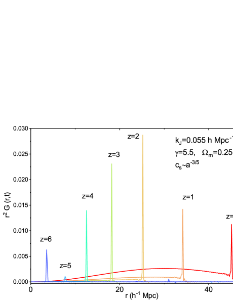
Figure 25: The Green’s function $G(r,t)$ as the solution of (B.8) is a spike at each instant, analogous to a delta function $\delta(r-c(t)t)$, and is propagating forward at a speed $c(t)$. The weighted $r^{2}G(r,t)$ is shown.

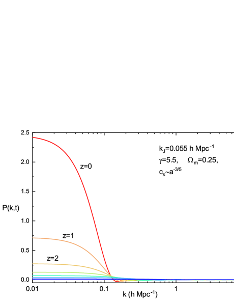
Figure 26: Same as Fig. 25. The power spectrum $P_{k}(t)$ associated with $G(r,t)$.

One sees that $G({\bf x,x_{0}},t)$ is a sharp spike located at $({\bf x-x_{0}})$ at instance $t$, like $\delta(|{\bf x-x_{0}}|-c(t)t)$, and is propagating forward at finite speed $c(t)$, which is quite similar to (B.9) in the simple case. After the $d\tau$ integration in (B.7), $w_{1}$ receives contributions from all the spherical surfaces of the radius $\leq c(t)t$, analogous to a step function, nonvanishing only within a region $r<c(t)t$. The inhomogeneous solution $\xi_{1}=w_{1}/a$ is the major part of the main mountain of $\xi$ at small scales, and is growing with time. This “retarded potential” behavior of $\xi_{1}$ is demonstrated in Fig.16.

The solution $w_{2}$ of (B.5) also can be expressed in terms of Green’s function. We decompose it into two parts,

$$w_{2}({\bf x},t)=u({\bf x},t)+v({\bf x},t),$$ (B.10)

where $u$ satisfies the following homogeneous equation with the initial velocity

$$\left\{\begin{split}&\ddot{u}({\bf x},t)-c^{2}(t)\nabla^{2}u({\bf x},t)-m^{2}(t)u({\bf x},t)=0\\ &u\big{|}_{t=t_{i}}=0\\ &\dot{u}\big{|}_{t=t_{i}}=a(t_{i})\Big{(}H(t_{i})\xi({\bf x},t_{i})+\dot{\xi}({\bf x},t_{i})\Big{)},\end{split}\right.$$ (B.11)

which has the same structure as (B.8) and the solution is

$$u({\bf x},t)=\int a(t_{i})\Big{(}H(t_{i})\xi({\bf x_{0}},t_{i})+\dot{\xi}({\bf x_{0}},t_{i})\Big{)}G({\bf x,x_{0}},t)d^{3}x_{0},$$ (B.12)

where $G({\bf x,x_{0}},t)$ is the Green’s function of (B.8). $u$ represents the contribution of the initial rate. Due to the property of $G({\bf x,x_{0}},t)$, the $d^{3}x_{0}$ integration receives most of contributions from a region around a spherical surface of radius $c(t)t$ centered at ${\bf x}$. $v$ in (B.10) satisfies the following equation with the initial value

$$\left\{\begin{split}&\ddot{v}({\bf x},t)-c^{2}(t)\nabla^{2}v({\bf x},t)-m^{2}(t)v({\bf x},t)=0\\ &v({\bf x},t)|_{t=t_{i}}=a(t_{i})\xi({\bf x},t_{i})\\ &\dot{v}({\bf x},t)\big{|}_{t=t_{i}}=0.\\ \end{split}\right.$$ (B.13)

By Duhamel’s principle, the solution is

$$v({\bf x},t)=v({\bf x},t_{i})+\int^{t}_{t_{i}}\Big{[}\int\Big{(}c^{2}(\tau)\nabla^{2}_{\bf x_{0}}v({\bf x_{0}},t_{i})+m^{2}(\tau)v({\bf x_{0}},t_{i})\Big{)}G({\bf x,x_{0}},t)d^{3}x_{0}\Big{]}d\tau,$$ (B.14)

where $G({\bf x,x_{0}},t)$ is the Greens’ function of (B.8). The homogeneous solution $\xi_{2}=(u+v)/a$ gives rise to the periodic bumps of $\xi$, whose amplitudes are growing during evolution, as seen in Fig.18, Fig.19, and Fig.20. $v$ is dominant over $u$ because the rates $H_{0}$ and $r_{a}$ are small. The sum of (B.7), (B.12), and (B.14) is the solution $\xi$ of Eq. (8) in terms of the Green’s function.

References

- [1] F. Beutler et al., Mon. Not. R. Astron. Soc. 416, 3017 (2011).
- [2] A. G. Sanchez et al., Mon. Not. R. Astron. Soc. 464, 1640 (2017).
- [3] L. Anderson et al., Mon. Not. R. Astron. Soc. 441, 24 (2014).
- [4] R. Ruggeri and C. Blake, Mon. Not. R. Astron. Soc. 498, 3744 (2020).
- [5] C. Blake et al., Mon. Not. R. Astron. Soc. 418, 1707 (2011).
- [6] E. A. Kazin et al., Mon. Not. R. Astron. Soc. 441, 3524 (2014).
- [7] M. Ata et al., Mon. Not. R. Astron. Soc. 473, 4773 (2018).
- [8] N. G. Busca et al., Astron. Astrophys. 552, A96 (2013).
- [9] J. E. Bautista et al. Astron. Astrophys. 603, A12 (2017).
- [10] A. Slosar et al., J. Cosmol. Astropart. Phys., 04 (2013) 026.
- [11] M. Davis and P. J. E. Peebles, Astrophys. J. Suppl. 34, 425 (1977).
- [12] W. C. Saslaw, Gravitational Physics of Stellar and Galactic Systems, (Cambridge Univ. Press, England, 1985); The Distribution of the Galaxies: Gravitational Clustering in Cosmology, (Cambridge Univ. Press, England, 2000).
- [13] H. J. de Vega, N. Sanchez, and F. Combes, Phys. Rev. D 54, 6008 (1996); Nature (London) 383, 56 (1996); Astrophys. J. 500, 8 (1998).
- [14] Y. Zhang, Astron. Astrophys. 464, 811, (2007).
- [15] Y. Zhang and H. X. Miao, Res. Astron. Astrophys. 9, 501 (2009); Y. Zhang, and Q. Chen, Astron. Astrophys. 581, A53, (2015); Y. Zhang, Q. Chen, & S. W. Wu, Res. Astron. Astrophys. 19, 53, (2019).
- [16] N. A. Bahcall, in Unsolved Problems in Astrophysics, edited by J. P. Bahcall, and J. P. Ostriker (Princeton Univ. Press, NJ, 1996); N. A. Bahcall, et al. Astrophys. J. 599, 814 (2003).
- [17] P. J. E. Peebles, The Large-scale Structure of the Universe. (Princeton Univ. Press, NJ, 1980).
- [18] B. Wang and Y. Zhang, Phys.Rev .D 96, 103522 (2017); Y. Zhang, F. Qin, and B. Wang, Phys.Rev .D 96, 103523 (2017); B. Wang and Y. Zhang, Phys. Rev. D 98, 123019 (2018); B. Wang and Y. Zhang, Phys. Rev. D 99, 123008 (2019).
- [19] N. Goldenfeld, Lectures on Phase Transitions and the Renormalization Group, (Addison-Wesley, MA, 1992).
- [20] J. G. Kirkwood, J. Chem. Phys. 3, 300 (1935).
- [21] E. J. Groth and P. J. E. Peebles, Astrophys. J. 217, 385 (1977).
- [22] J. N. Fry and P. J. E. Peebles, Astrophys. J. 221, 19 (1978).
- [23] J. Binney and S. Tremaine, Galactic Dynamics, (Princeton Univ. Press, NJ, 1987).
- [24] J. Jeans, Phil. Trans. R. Soc. A 119, 49 (1902).
- [25] G. Gamow and E. Teller, Phys. Rev. 55, 654 (1939).
- [26] W. Bonnor, Mon. Not. R. Astron. Soc. 117, 104 (1957).
- [27] P. J. E. Peebles, Principles of Physical Cosmology, (Princeton Univ. Press, NJ, 1993).
- [28] V. Springel et al. Mon. Not. R. Astron. Soc. 475, 676 (2018).
- [29] R. A. Sunyaev and Ya. B. Zel’dovich, Astrophys. Space. Sci. 7, 3 (1970).
- [30] P. J. E. Peebles and T. J. Yu, Astrophys. J. 162, 815 (1970).
- [31] J. Silk, Astrophys. J. 151, 459 (1968).
- [32] G. B. Field, Astrophys. J. 165, 29 (1971).
- [33] S. Weinberg, Astrophys. J. 168, 175 (1971).
- [34] S. Weinberg, Gravitation and Cosmology, (John Wiley & Sons, Nre York, 1972).
- [35] J. A. Holtzman, Astrophys. J. 71, 1 (1989).
- [36] W. Hu and N Sujiyama, Astrophys. J. 444, 489 (1995); Astrophys. J. 471, 542, (1996).
- [37] D. J. Eisenstein and W. Hu, Astrophys. J. 496, 605, (1998).
- [38] E. Hawkins et al. Mon. Not. R. Astron. Soc. 346, 78 (2003).
- [39] H. Totsuji, and T. Kihara, Publ. Astron. Soc. Jpn 21, 221 (1969).
- [40] P. J. E. Peebles, Astrophys. J. 189, L51 (1974).
- [41] P. J. E. Peebles, Astron. Astrophys. 32, 197 (1974).
- [42] Y. Zhang, X. Ye, and B. Wang, Sci. Chin. Phys. Mech. Astron. 63, 250411 (2020). arXiv:gr-cg/1903.10115.
- [43] Y. Zhang, B. Wang, and X. Ye, Chin. Phys. C. 44, 1 (2020). arXiv:gr-cg/1909.13010.
- [44] T. J. Broadhurst, R.S. Ellis, D.C. Koo, and A.S. Szalay, Nature (London) 343, 726 (1990).
- [45] T. J. Broadhurst et al. in Wide Field Spectroscopy and the Distant Universe, eds. S.J. Maddox and A. Arag’on-Salamanca, (World Scientific Publishing, 1995).
- [46] D. L. Tucker et al. Mon. Not. R. Astron. Soc. 285, L5 (1997).
- [47] J. Einasto et al. Nature (London) 385, 139 (1997).
- [48] J. Einasto et al. Mon. Not. R. Astron. Soc. 289, 801 (1997).
- [49] J. Einasto, in The Ninth Marcel Grossmann Meeting, Proceedings of the MGIXMM Meeting, eds. V. G. Gurzadyan, R.T. Jantzen, and R. Ruffini, (World Scientific Publishing, Singapore, 2002).
- [50] M. Einasto et al. Astron. J. 123, 51 (2002).
- [51] E. Tago et al. Astron. J. 123, 37 (2002).
- [52] L. Anderson et al. Mon. Not. R. Astron. Soc. 427, 3435 (2012).
- [53] V. d. S. Agathe, Astron. Astrophys. 629, A85 (2019).
- [54] K. Yahata, et al., Publ. Astron. Soc. Jpn 57, 529 (2005).
- [55] J. Einasto, G. Hutsi , T. Kuutma, and M. Einasto, Astron. Astrophys. 640, A47 (2002).
- [56] P. H. Chavanis, Physica A, 361, 55 (2006).
- [57] D. J. Eisenstein et al. Astrophys. J. 633, 560 (2005).
- [58] D. H. Weinberg et al. Physics Report 530, 87 (2013).
- [59] J. M. Bardeen, J. R. Bond, N. Kaiser, and A. S. Szalay, Astrophys. J. 304, 15 (1986).
- [60] B. Allen, in Proceedings of the Les Houches School of Physics, edited by J.A. Marck and J.P. Lasota, 26: 373 (Cambridge University Press, 1997), arXiv:gr-qc/9604033 ; B. Allen and J. D. Romano, Phys. Rev. D 59, 102001 (1999).
- [61] Bo Wang and Yang Zhang, Res. Astron. Astrophys. 19, 24 (2019).
- [62] S. Bashinsky and E. Bertschinger, Phys. Rev. D 65, 123008 (2002).
- [63] C. Hernandez-Aguayo et al. Mon. Not. R. Astron. Soc. 494, 3120 (2020).
- [64] M. C. Neyrinck et al. Mon. Not. R. Astron. Soc. 478, 2495 (2018).
- [65] B. D. Sherwin and M. Zaldarriaga, Phys. Rev. D 85, 103523 (2012).
- [66] N. D. Spergel et al. Astrophys. J. Suppl. 170, 377 (2007).
- [67] J. Dunkey et al. Astrophys. J. Suppl. 180, 306 (2009).
- [68] M. Reid, D. Pesce, and A. Riess, Astrophys. J. Lett. 886, L27 (2019).
- [69] D. Pesce et al. Astrophys. J. Lett. 891, L1 (2020).
- [70] K. C. Wong et al., Mon. Not. R. Astron. Soc. 498, 1420 (2020).
- [71] P. A. R. Ade et al. (Planck Collaboration), Astron. Astrophys. 594, A13 (2016).
- [72] N. Aghanim et al. (Planck Collaboration), Astron. Astrophys. 641, A6 (2020).
- [73] L. D. Landau and E. M. Lifshitz, Fluid Mechanics, (Pergamon Press, New York, 1987).
- [74] J. J. Binney, N. Dowrick, A. Fisher, and M. Newman, The Theory of Critical Phenomena, (Oxford Univ. Press, New York, 1992).
- [75] J. Zinn-Justin, Quantum Field Theory and Critical Phenomena, (Oxford Univ. Press, New York, 1996).
- [76] O. Lahav, P. B. Lilje, J. R. Primack, and M. J. Rees, Mon. Not. R. Astron. Soc. 251, 128 (1991).