Data Synthesis for Testing Black-Box Machine Learning Models

Abstract.

The increasing usage of machine learning models raises the question of the reliability of these models. The current practice of testing with limited data is often insufficient. In this paper, we provide a framework for automated test data synthesis to test black-box ML/DL models. We address an important challenge of generating realistic user-controllable data with model agnostic coverage criteria to test a varied set of properties, essentially to increase trust in machine learning models. We experimentally demonstrate the effectiveness of our technique.

1. Introduction

Artificial Intelligence systems are increasingly being used in critical applications, such as to assess a criminal defendant’s likelihood of committing a crime (Dressel and Farid, 2018), selecting resumes for recruitment (Cowgill, 2017), loan processing (Mukerjee et al., 2002), etc. While AI holds the promise of delivering valuable insights and knowledge across a multitude of applications, the broad adoption of AI systems will rely heavily on the ability to trust their output.

In order to assure the reliability of AI systems, in this paper, we address some of shortcomings of automated testing of AI models, as described below.  The data scientists use the technique of splitting the cleaned data to get train and test set in order to build and select the best model in terms of accuracy. In industry, Model Risk Management (MRM, 2020) phase of the Data and AI lifecycle independently tests the model on various characteristics such fairness, robustness, drift, and business KPIs before deploying the model. Such risk management imposes the following additional requirements.

• Risk management requires additional realistic test data, not used by data scientists as the available test split may not be a complete representation of the possible payload data making it insufficient.

• Simulation of anticipatory data-drift condition to generate synthetic payload to test the model under such data distribution drift.

• As the above requirements warrants generation of synthetic test data, it is important to generate the data based on some coverage criteria suitable for AI testing.

• Use of synthetic test data to test fairness [18,44], robustness [7,28] properties in AI model which is majorly skipped by current industrial practices.

Although existing techniques like GAN (Goodfellow et al., 2014), Variational Auto-encoder (Kingma and Welling, [n. d.]) can generate synthetic realistic data, they are not customizable by user-specification. Moreover, existing coverage criteria like neuron coverage, sign coverage, boundary value coverage, etc.  (Pei et al., [n. d.]; Ma et al., [n. d.]) are not model-agnostic and cannot be combined with existing generative models.

To address the majority of the above-mentioned drawbacks, we build a testing framework, called AITEST. The salient features of our framework are listed next.

• First, to address the limited test data, we develop a technique to synthetically generate realistic test data. For example, if there are two columns like age and marital-status - a random generation technique can generate married people younger than 20 even though such as behavior is not present in the training data. Our data synthesis technique ensures that such a case never occurs. Specifically, the generated data (without any customization) has the similar statistical characteristics of the training data.

• Second, our synthetic data generation process is customizable. Consider a case where the training data is taken from a North America region where Male-Female ratio is, say 3:2, which is captured as a constraint inferred from the training data. To cater to the testing for a different geographic region that has a different Male:Female (say 1:1), it is important to test the fairness metric with such synthetic data. AITEST allows to incorporate user-defined constraints (UDC) to add and/or update the data constraints. The UDC is also important to capture any domain-based constraints which are hard to infer from the data or expected payload characteristics. The flexibility of having UDC is important from an AI Testing perspective to test various unprecedented what-if scenarios even before deploying the model in production.

• Third, to cater to the challenge of defining a model-agnostic coverage criterion, we re-use the notion of program path coverage. However, the notion of paths cannot be defined for all models. Therefore, we introduce the notion of model-agnostic path-coverage and present algorithms for test-data synthesis ensuring high coverage. Essentially, we create a decision tree model with high fidelity which imitates the model under test. The test cases are then, equally distributed in the regions defined by the constraints in each path (hereafter called path-constrains) in the decision tree. Coverage of paths in the decision tree ensures decision region coverage of the model under test.

• AITEST performs goal-oriented test data synthesis. We perform group/individual fairness and robustness testing which are metamorphic properties (Xie et al., 2011) whose testing does not require an oracle to get label for synthetic data.

The current scope of our system is classification models for tabular data. To the best of our knowledge, no other techniques address this in tabular domain. Ribeiro et al. demonstrated the importance of testing NLP models in (Ribeiro et al., 2020). Our contributions are listed below:

• We develop an algorithm to generate realistic test data which is cutomizable giving the user an opportunity to perform drift-testing.

• We define a model-agnostic path coverage criteria and re-use an existing global explainability algorithm to generate the data offering maximum coverage.

• Our technique tests fairness and robustness with realistic synthetic data which is not done by other realistic synthetic test data generation techniques.

2. Background

In this section, we present the background of some of the already known concepts that we use in our framework.

Decision Tree Surrogate

We use an algorithm, called TREPAN (Craven, 1996) to create a decision tree surrogate of any given model with black-box access for defining its coverage. Essentially, TREPAN uses training data with model predictions (instead of ground truth) to imitate the decision logic of the black-box model with a decision tree (an interpretable model). TREPAN also generates random synthetic samples when the number of training samples for an intermediate node in the decision tree is reduced below a given threshold. Note that it uses the labels from the target classifier even for those synthetically generated samples. The use of these additional samples helps to create a better surrogate.

Fairness

A fair classifier tries not to discriminate individuals or groups defined by the protected attribute (like race, gender, caste, and religion) (Aggarwal et al., 2019). Next, we describe metrics related to group fairness (between two groups) and individual fairness (between two individuals) by using the following notations. Each sample/individual is denoted as ($X$, $Y$, $Z$) where $X$ are all attributes used in the prediction, $Y$ is the corresponding ground-truths for the samples in $X$, and $Z$ is the binary protected attribute which may be included in $X$. A classifier is a mapping $h$: $X\rightarrow[0,1]$. The final prediction is denoted by $\hat{Y}$ where $\hat{Y}=1\Leftrightarrow h(X)>\sigma$. We will use $P({\hat{Y}=1}|Z=1)$ as the probability of a favorable outcome ($\hat{Y}=1$) for the privileged group ($Z=1$).

Group Fairness. Below we recall some prominent group discrimination metrics that we use. Under the definition of disparate impact (Feldman et al., 2015), a system is fair if:

$\dfrac{P(\hat{Y}=1|Z=0)}{P({\hat{Y}}=1|Z=1)}>\epsilon$. In other words, the probability of the favorable outcome of the unprivileged and privileged group should be more than a particular threshold. Typically, based on US Govt. rules, in many scenarios $\epsilon=0.8$.

Individual Fairness. Based on the notion of counterfactual fairness (Kusner et al., 2017), a decision is fair towards an individual if it is the same in (a) the actual world and (b) a counterfactual world where the individual belonged to a different demographic group. Essentially, a test case corresponding to individual fairness consists of a pair of samples where the two samples only differ in protected attribute values - one from the privileged group and the other from the unprivileged group. Formally, $h(s)<\epsilon$ and $h(s^{\prime})\geq\epsilon$ where $s.Z\neq s^{\prime}.Z$ and $s.y=s^{\prime}.y~{}\forall y\in Y$.

Note that just removing the protected attribute from the training data doesn’t ensure fairness in AI models due to the existence of possible indirect bias (Aggarwal et al., 2019), and therefore such a testing is required. Further, our testing framework is generic enough to work for any other definition of fairness, but currently we are using the one used in  (Galhotra et al., [n. d.]) (Udeshi et al., 2018) (Aggarwal et al., 2019).

Adversarial Robustness

Testing for adversarial robustness consists of creating two realistic samples based on some perturbation function $p$ and checking if both of them give different outcomes (test failure).

3. Data Synthesis

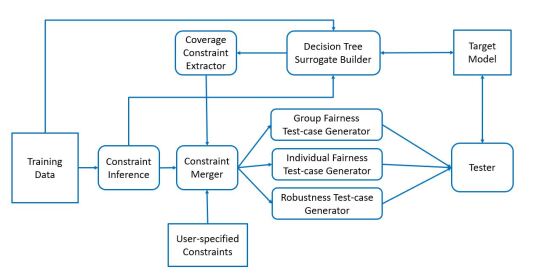
Figure 1. AITEST Architecture

Figure 1 shows the different components of AITEST architecture and how they interact with each other. At first, AITEST processes the training data to obtain a set of constraints. Using such constraints, AITEST can generate synthetic data using a new constraint solver, after optionally merging user-defined constraints and path constraints. Finally, it generates the test cases for specific properties which are fed to testers. This section discusses different components of AITEST in detail.

3.1. Constraints

The first step is to understand each column in the given data and find associations between different type of columns. Note that we ignore the label column in this phase. As per our constraint language specified in Table 1, constraints are of two types - column constraints which are defined for each column, and association constraints which are defined based on more than one column.

Column Constraints. We assume that a column can have either numeric or category datatype, the latter having a fixed set of unique values. Based on the column’s datatype, different kinds of distribution constraints are inferred. For each category column, AITEST gathers frequency distribution of all the unique set of values, whereas for numeric column, AITEST gathers statistical properties such as minimum-maximum bound and various statistical distributions. Note that we try to fit five common statistical distributions for numeric columns - $uniform$, $normal$, $beta$, $exponential$ and $gamma$, using Scipy’s distribution fit (scipy-2020, 2020) that uses maximum likelihood estimation technique, and then use the Kolmogrov Smirnov (KS) test (Kolmogorov, 1933; Massey, 1951) to check which distribution fits the column best. KS test compares the data with a reference probability distribution, and measures the distance between empirical distribution function of the sample and cumulative distribution function of the reference distribution. The KS statistic value (or $p$-value) is high (1) when the fit is good, and low (0) otherwise. The lack of fit is significant if $p$-value $<$ $0.05$. We say that a distribution fits the column if $p$-value from the KS test $>$ $0.05$ and is the best amongst the distributions checked. Due of this check, a numerical column may not have any associated distribution.

Table 1. Constraints

$constraints$	::=	$column~{}~{}|~{}~{}association$
$column$	::=	$categorical~{}~{}|~{}~{}numerical$
$categorical$	::=	$frequency\_distribution$
$numerical$	::=	$statistical~{}~{}|~{}~{}distributions$
$statistical$	::=	$min~{}~{}|~{}~{}~{}max$
$distributions$	::=	$normal~{}~{}|~{}~{}uniform~{}~{}|~{}~{}beta$
		$exponential~{}~{}|~{}~{}gamma$
$association$	::=	$cat\_cat~{}~{}|~{}~{}cat\_num$
$cat\_num$	::=	$\forall v\in categorical,(v,numerical)$
$cat\_cat$	::=	$\forall v\in categorical,(v,categorical)$

Associations. We aim to capture two types of relationships involving a pair of source and target column. The cat_cat is defined between two category columns. We perform Chi-square($\chi^{2}$) test (Pearson, 1900) and use uncertainty coefficient, Thiel’s U (Theil, 1970) to measure independence between categorical attributes to identify the source and target column. Thiel’s U is based on the conditional entropy between two nominal attributes and measures the degree of association from the source to target, with the value in range $[0,1]$, where $0$ means no association and $1$ represents a full association. We capture the frequency distribution of values in the target column for each unique value-combination in the source column. The cat_num association is defined between a category source and a numeric target column. For every unique value in the source category column, we find column-level constraints for the filtered samples in the target numeric column. For numeric target column, we do not represent joint categorical source columns in the association constraint as the count of numerical samples becomes very less for each value-combination of source categorical columns which prohibits distribution fit. However, our synthesis phase (described later) partially considers all the cat_num association constraints for a numerical column.

Note that the datasets are generally preprocessed before training a model and therefore, all the redundant columns or columns dependent on other columns are pruned. Hence, an association from a numeric column to another numeric one capturing a polynomial relationship may not be useful, especially for testing ML models. Furthermore, it is also possible to define many other constraints, for example, associations defined by considering more than two columns. But, we found the suggested set of constraints enough and best suited for our data synthesis technique.

To capture the dependency between all the constraints, we define a directed graph, $G(N,E)$ and call it the Constraint Dependency Graph ($CDG$). Each node $n\in N$ in this $CDG$ corresponds to a feature/column and is annotated with an associated inference error related to individual feature constraints. This $inf\_error(n)$ is $0$ for categorical columns and numerical columns where no distribution is inferred. For a numerical column $n$ having some distribution, $inf\_error(n)=1-p$-value. Each directed edge $e\in E$ in the graph corresponds to either a cat_num association or part of cat_cat association between source and target node. Edge $e$ is annotated with $inf\_error(e)$ which is $1-u$-value for cat_cat edges, where $u$-value is the uncertainty coefficient for $e$, and for each cat_num edge, it is an average of numerical distributions errors for all category source values. Since a numerical column may not have any continuous distribution function in feature constraint (but may have association), each node is classified into two types - 1) GenNode: one having distribution function and 2) NonGenNode: not having any distribution function. Later, we demonstrate how to use this $CDG$ for data synthesis.

Consider a toy dataset with five categorical attributes (gender, education, martial, age-grp, intelligence) and one numeric attribute (salary) with relevant associations between them. An exemplar $CDG$ is shown in Figure 2 (G1).

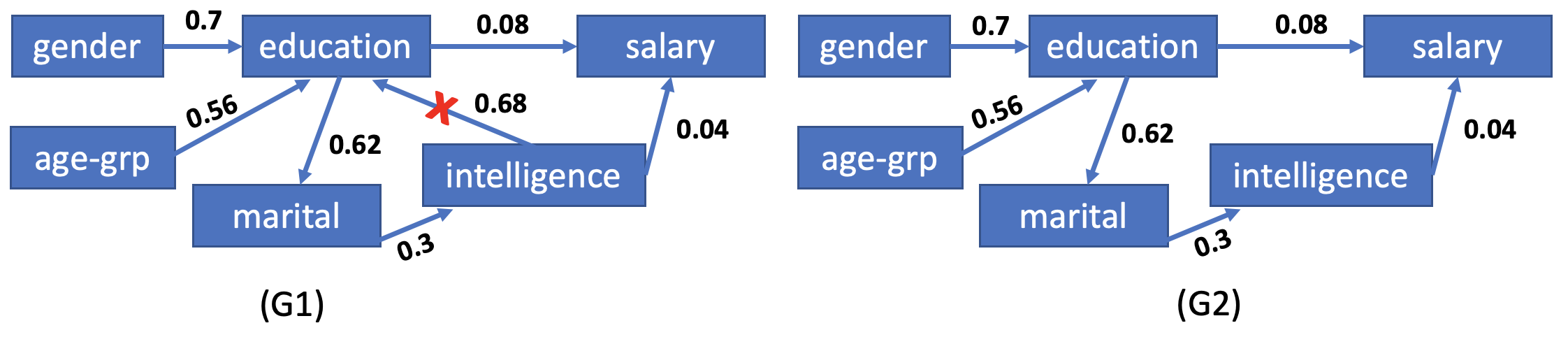
Figure 2. CDG (G1) and DAG (G2)

3.2. User-Defined Constraint Specification

Apart from the data constraints, AITEST also enables a user to add new constraints or delete/modify the existing data constraints in form of user-defined ones (UDC) which take precedence over the existing data constraints. Our specification supports three types of UDCs as listed below.

• Add UDC - User can add constraints which spans both association and column related constraints. For example, if data constraints infer that values of salary lie in the range [2k-30k] with no distribution, then, using UDC, user can override this random generation by specifying, say a normal distribution with loc=15k and scale=0.1 lying in the same bounds [2k-30k].

• Modify UDC - User can specify constraints to modify/override the existing data constraints, both association and feature related constraints, as in the usage scenarios below.
  Range Modification - Let’s consider that the user wants to generate salary values for females in a particular range, say, 5k-50k, which is different from the bounds 2k-30k as specified in cat_num association between gender and salary. Using user-defined constraints, he/she can override the value bounds or statistical distribution in feature/associations constraints with the desired values.
  Distribution Modification - Another scenario of its utility can be when the user wants to generate test cases to check for group fairness in AI model. For a protected attribute, say gender, the frequency distribution of M:F is, say 3:1, in the feature constraint. But, it may be desired to check for fairness with the test set having a different relative proportion of M and F, say 1:1. Our UDC template allows such frequency distribution overriding.

• Delete UDC - User can ask the system to drop certain associations or feature constraints from the inferred data constraints during test data synthesis. For instance, drop range constraints on an attribute, or drop associations between a protected (gender) and non-protected (salary) attribute during test data generation.

Later in Section 3.3, we discuss the way to handle such UDCs in our synthesis algorithm.

3.3. Realistic Data Synthesis

1

2 Function DataSynthesis(InputData, n)

3       DataConstraints = genConstrains(InputData)

4       CDG = createCDG(DataConstraints)

5       return DataSynWithDataCons(CDG, n)

6      

7 end

8

9Function createCDG(DC, n)

10       G.nodes = {}

11       G.edges = {}

12       foreach $c\in DC.columns$ do

13             G.nodes += $n_{c}$

14       end foreach

15      foreach $fc\in DC.feature\_constraints$ do

16             $n_{c}.constraints$ += $fc$

17             if ($n_{c}.type==NUM\wedge\exists c\in fc~{}s.t.~{}c.type==cont\_distribution$) then

18                   $n_{c}.GenNode=False$

19            else

20                   $n_{c}.GenNode=True$

21             end if

22            

23       end foreach

24      foreach $ac\in DC.assoc\_constraints$ do

25             $n_{c}.asso\_constraints$ += $ac$

26       end foreach

27      return G

28 end

29Function DataSynWithDataCons(CDG, n)

30       DAG = preProcess(CDG)

31       return generate(DAG, n)

32 end

33Function preProcess(CDG)

34       DAG = CDG.copy()

35       while $\exists~{}directed~{}cycle~{}$c$\in DAG$ do

36             delete edge ($n_{i},n_{j}$) with minimal confidence s.t. $n_{j}.GenNode=True$

37       end while

38      return DAG

39 end

40

41Function DataSynWithDataCons(DAG, n)

42       while $n_{j}\in topologicalOrder(DAG.nodes)$ do

43             data = genDataEachColumn($n_{j}$, DAG, n)

44             $n_{j}.data=data$

45       end while

46      

47 end

48Function genDataEachColumn($n_{j}$, DAG, n)

49       if ($n_{j}.GenNode\wedge n_{j}.type==NUM$) then

50             dataOwn = gen($n_{j}$.dist, n, $n_{j}$.range, $n_{j}$.isUnique)

51             minDiv = +Inf

52             minDivData = null

53             foreach (e = ($n_{i}$,$n_{j}$) do

54                   data=genData(e,$n_{i}$)

55                   div = KL-div(dataOwn, data)

56                   if $div<minDiv$ then

57                         minDivData = data

58                        

59                   end if

60                  

61             end foreach

62            $n_{j}.data=data$

63            

64      else if ($n_{j}.GenNode$) then

            

             // type CAT

65             e = ($n_{i}$,$n_{j}$) for any $n_{i}$

66             data=genData(e,$n_{i}$)

67             $n_{j}.data=data$

68            

69      else

            

             // NonGenNode

70             e = ($n_{i}$,$n_{j}$) s.t. $error(e)$ is min for all $n_{i}$

71             data=genData(e,$n_{i}$)

72             $n_{j}.data=data$

73            

74       end if

75      

76 end

77

Algorithm 1 Data Synthesis using Data Constraints

In this section, we present the overall algorithm of data synthesis in three stages - starting from realistic data synthesis from data constraints, and subsequently adding user-defined constraints and coverage constraints. Furthermore, the synthesizer also expects the count of samples to be generated as an input. Note that the synthesizer does not generate data for the label column.

In order to generate values for the toy example, we need to consider the following set of constraints.

1. Feature Constraints of individual attributes

   • Continuous Marginal Distribution: Synthesizer can generate values by sampling from the existing distribution e.g. salary from normal distribution.

   • Discrete Marginal Distribution: Synthesizer can generate required number of values for a fixed frequency ratio (e.g. gender in a, say M:F=2:1) using enumeration.

2. Association Constraints

   • Conditional Distribution for Numerical variables (cat_num): Using sampling from the distribution for specific categorical values. For education=masters, if salary follows a uniform distribution with specific bounds, then for every masters value, we can sample a value from this distribution for salary.

   • Conditional Distribution for Categorical variables (cat_cat): For each value-combination of gender, age-grp in source, say {Female, Senior}, the frequency distribution of target education (say primary:secondary:tertiary=1:2:3) is used to generate synthetic values for education for all rows containing {Female, Senior}.

But, the challenge is how to generate values for an attribute while considering multiple constraints at once.

Data synthesis for a node can be done in two ways - either by using the generation procedure for feature distributions (marginal distributions) or by solving the association constraint in each incoming edge whose source values have already been generated (conditional distribution). This essentially outlines the challenges in our data synthesis algorithm - 1) the order of processing the nodes through $CDG$, and 2) how to compute the data for each node.

Note that the $CDG$ can contain cycles involving three or more nodes. To address the node processing problem, the synthesizer pre-processes the $CDG$ to remove any cycles, essentially turning it into a directed acyclic graph (DAG) (Graph G2 in Figure 2). The synthesizer breaks a cycle by removing any one incoming edge to a GenNode with maximal error in the cycle. This is because a NonGenNode requires an association constraint to generate its value and removing the most-erroneous edge ensures that less error is propagated through the graph. Once the DAG is obtained, the generation proceeds node-by-node in topological order or bottom-up order in the DAG.

Assuming that there is no singleton disconnected node in the graph, this transformation leads to a DAG which has only GenNodes in the leaves. The synthesizer generates values in the leaves using the marginal distribution-based generation procedure described before. Subsequently, the generation proceeds through the DAG in the topological order starting from the leaves, generating values for each non-leaf node.

Consider a case, where a non-leaf node has a single incoming edge. In this case, it is easy to see that considering the association constraints to compute the data (as described before) is better with respect to its own distribution as it incurs zero loss for categorical columns and minimal distribution loss for the numeric columns while also respecting the relationship with the other feature values.

In the case of multiple incoming edges, there are three cases. If the current node $n$ is a GenNode and numeric, then for every incoming edge $e$ (of type cat_num), the synthesizer generates data and computes KL-divergence error (Kullback and Leibler, 1951) ($kl\_error(e)$) with respect to its own distribution in column constraints. It finally selects the edge $e^{\prime}$ having minimal kl_error. Based on ($e^{\prime}=(cat,n)$), it samples data from the numerical distribution corresponding to every categorical value of variable $cat$. For each such generated value of $n$, it accepts the samples only if ($\forall e^{\prime\prime}=(cat^{\prime},n),e^{\prime\prime}!=e$) the range constraints for $e^{\prime\prime}$ are also satisfied, thereby minimizing the difference from his own distribution while maintaining cross-feature relationships. For example, salary is generated by the distribution corresponding to each education value, but the generated value also respects the salary range of the corresponding intelligence value. If this node $n$ is a GenNode but categorical, it uses cat_cat relationship involving multiple source nodes to compute the data. In the third case, i.e. for a NonGenNode, the synthesizer selects the incoming edge with minimum error ($error(e)$) and computes the data. We define error of node $n$ and edge $e$ as follows.

$$error(n)=\begin{cases}inf\_error(n),\text{if $n$ is a leaf-node},\\ error(e^{\prime})+kl\_error(e^{\prime})\times inf\_error(n),\text{ow.}\end{cases}$$

where $error(e)=inf\_error(e)+error(n^{\prime})$ when $n^{\prime}$ is source of $e$, and $e^{\prime}$ is the incoming edge selected to generate values of node $n$. Essentially, this synthesis error of node $n$ is propagated to all the outgoing edges in the graph. The pseudo-code of our realistic data synthesis algorithm is presented in Algorithm 1.

In the above example, the order of processing nodes is gender, age-grp, education, marital, intelligence, and salary. The synthesizer applies the case of multiple incoming edges for the education and salary nodes.

1

2

3Function DataSynWitUDC(CDG, n, UDC)

4       DAG = preProcessWithUDC(CDG, UDC)

5       return DataSynWithDataCons(DAG, n)

6 end

7Function preProcessWithUDC(CDG, UDC)

8       DAG = CDG.copy()

9       DAG = processUDC(DAG, UDC)

10       while $\exists~{}directed~{}cycle~{}c\in DAG$ do

11             delete edge $e=(n_{i},n_{j})$ with minimal confidence s.t. $n_{j}.GenNode=True$ where

12       end while

13      return DAG

14 end

15Function processUDC(DAG, UDC)

16       foreach $c\in UDC.Add$ do

17             delete $c$ from $DAG$

18            

19       end foreach

20      foreach $c\in UDC.Add$ do

21             if $c=n_{c}.cons$ is a feature constraint then

22                   Add to the corresponding node $n_{c}$ in $DAG$

23                   remove incoming edges to $n_{c}$

24             end if

25            if $c=(n_{i},n_{j}).cons$ is an association constraint then

26                   Add to $(n_{i},n_{j}).cons$ to $DAG$

27                   remove other incoming edges to $n_{j}$

28                  

29             end if

30            

31       end foreach

32      foreach $c\in UDC.Modify$ do

33            

34            if $c=n_{c}.cons$ is a feature constraint $\wedge$ of type distribution then

35                   Modify the corresponding node $n_{c}$ in $DAG$

36                   remove incoming edges to $n_{c}$

37            else if $c=(n_{i},n_{j}).cons$ is an association constraint $\wedge$ then

38                   Modify $(n_{i},n_{j}).cons$ im $DAG$

39                   remove other incoming edges to $n_{j}$

40                  

41            else

42                   $c=n_{c}.cons$// Update constraints in node $n_{c}$ DAG// Make it high confidence

43             end if

44            

45       end foreach

46      return DAG

47 end

48

Algorithm 2 Data Synthesis using Data Constraints and User-defined constraints

Handling User-Defined Constraints (UDCs)

If user specifies some additional constraints to override the existing ones obtained from data, then the synthesizer first merges the two set of constraints. This resultant merged constraint set is then used to synthesize test data by a modification of the above process, as shown in Algorithm 2. Essentially, UDC nodes are made leaf node in the DAG by removing all the incoming edges. Also, the effect of UDC generated data is propagated through the DAG in such a way that it overrides any incoming edge selection choice described above.

UDCs are merged with data constraints with the existing data constraints, as below. Note that the UDCs have higher priority than the inferred data constraints.

• Add/Modify UDCs - For every such UDC, we add/modify that constraint in our set of data constraints. In case of conflict, we record the over-riding constraints in our data constraints and make sure that the former get precedence over the latter during the synthesis process.
  - Range modification - Note that there is a need to handle the cases of range modification in a more systematic way. Consider a case where data constraints have a feature constraints on an attribute, say salary, where the values are bounded by range $(min_{data},max_{data})$, say 2k-30k and follow a uniform distribution with certain parameters. Now, user specifies to override just the range for Salary as $(min_{user},max_{user})$, say 5k-50k without any change in associated statistical distribution. Overriding just the bounds in the data constraints may impact the present distribution parameters. Therefore, using the original min-max bounds 2k-30k along with the specified uniform distribution parameters in the data constraints, we first generate a set of salary values, V. We then scale these generated values using the below formula for every value v $\in$ V to the final output values for salary.

  $$v_{scaled}=min_{user}+\frac{(v-min_{data})*(max_{user}-min_{user})}{(max_{data}-min_{data})}$$

  This scaling ensures that the mean of scaled values is linearly scaled version of the values before scaling.

• Delete UDC - If the overriding constraints specify to drop an entire feature, $f$ from the resultant test set, then we drop the column constraints along with all its related association constraints where $f$ is mentioned as either source or target.

Path Coverage Constraints

The key idea here is to build a decision tree of the target model (in a model agnostic way) and use its path coverage as the coverage criteria for the target model. AITEST uses the TREPAN algorithm (Craven, 1996) to create a surrogate decision tree (see Section 2). TREPAN generates random data to augment the input training samples. We essentially change this step to generate realistic data instead of using random data. All path constraints are fetched for each path. The aim is to generate data satisfying the path constraints and satisfying majority of the data and UDC. Below, we describe the change in the above procedure to generate $n$ samples belonging to a path.

Each constraint in a path is either an equality predicate for categorical value or range constraints for numeric values. The columns with equality predicate are made leaf node in the CDG by deleting all incoming edges. However, the range constraints are added to the CDG nodes as additional feature constraints. Similar DAG generation and topological generation order starts with one necessary modification - only in the case where a range constraint does not agree with the association constraints, then the association constraints are ignored and the data is generated by considering the feature and range constraints.

1

2

3Function accuracy(n, CDG, UDC, DT, Model)

4       data = DS(CDG, n, DT, UDC)

5       label = labeler(data)

6       label1 = test(data)

7       return accuracy(label,label1)

8      

9 end

10Function group_fairness(model, n, CDG, UDC, DT, protected_attribute, priv_expr, fav_outcome, metrics)

11       result = []

12       data = DS(CDG, n, DT, UDC)

13       label1 = test(data, model)

14       foreach $metric\in metrics$ do

15             metric,value = evaluate(metric, data, label, protected_attribute, priv_expr, fav_outcome)

16             add (metric,value) to result

17            

18       end foreach

19      return result

20      

21 end

22

23Function individual_fairness(model, n, CDG, UDC, DT, protected_attribute, priv_expr, fav_outcome)

24       data = DS(CDG, n, DT, UDC)

25       indiv_algo(data, model,protected_attribute, priv_expr, fav_outcome, DS)

      

       // indiv_algo can be any off-the-shelf algorithm to detect individual discrimination

26      

27 end

28

29Function robustness(model, n, CDG, UDC, DT)

30       failure_count = total_failure_count = 0

31       data = DS(CDG, n, DT, UDC)

32       labels = test(data, model)

33       foreach sample $\in$ data do

34             data1 = perturb(sample)

35             labels1 = test(data1, model)

36             flag=0

37             foreach label $\in$ labels1 do

38                   if labels[sample]!=label then

39                         if !flag then

40                               failure_count++;

41                               flag = 1

42                              

43                         end if

44                        total_failure_count++;

45                   end if

46                  

47             end foreach

48            

49       end foreach

50      return total_failure_count, failure_count/—data—

51      

52 end

Algorithm 3 Property-based Test Data Synthesis

3.4. Property-based Test Data Synthesis

We further intend to generate realistic test cases to test an input AI model for a number of properties, namely Individual Fairness, Group Fairness and Robustness. Note that, all these properties are metamorphic in nature which do not require any oracle to tell the gold standard label for the synthetic test data. We use the same base approach as presented above with a few changes depending on the property, as shown in Algorithm 3. For property-based testing, AITEST takes data constraints, required test size, class label and protected attribute as an input.

The property-based test input generation starts with removing the feature related to input class label along with all the association constraints where this feature is specified as either a source or target. This ensures that any approximation caused due to constraint inference or synthesis does not seep into the prediction labels for these test inputs.

3.4.1. Individual Fairness Test Case Generator

We generate a set of synthetic samples using the synthetic test case generation procedure. For each sample, we change the predefined set of protected attribute (like race/gender) to create pair of test cases and which are checked against the model for label match. This closely resembles with the approach mentioned in (Galhotra et al., [n. d.]) which generates random samples (in comparison to our realistic samples) and subsequently perturbs them. Once a discriminatory sample, $s$ is found, we generate further more test inputs in its neighborhood using the below perturbation function $p$. We use an off-the-shelf explainer LIME (Ribeiro et al., 2016) to get a set of top (say $50\%$) attributes, $X^{\prime}$ such that $X^{\prime}$$\subset$$X$, contributing to the explanation of test $s$. For every prominent attribute, say $x^{\prime}$$\in$$X^{\prime}$, we then generate further more local test inputs as per the below scheme based on its datatype.
Categorical: Perturb $s.x^{\prime}$ for all possible values of $x^{\prime}$ to generate more tests.
Numerical: Generate inputs by perturbing $s.x^{\prime}$ for all integers or floats in range [$s.x^{\prime}$- $\delta$, $s.x^{\prime}$+$\delta$]. We have set $\delta$ as $3$ in our case. It is to be noted that the perturbation in such cases are bounded by the minimum and maximum permissible bounds of attribute as inferred from data constraints.

3.4.2. Group Fairness Test Case Generator

Specifically just for the group fairness use case, we unconditionally make the protected attribute independent by removing all those associations from the data constraints where it is mentioned as the target. This is done to ensure that the protected attribute in resultant synthetic test inputs follow the same frequency distribution as that of the input training data set. For example, if gender in the training data has composition of M:F in the ratio 2:1, then, it is desirable to test the model for group fairness with the test cases having same 2:1 M:F ratio. Note that this frequency distribution of protected attribute can be over-ridden by means of user-specified constraints as well as mentioned earlier in Subsection 3.2.

3.4.3. Robustness Test Case Generator

For every realistic test sample $s$, we perform robustness testing of the input model by generating more inputs in its neighbourhood, and checking if the predictions of any neighbour is different than that of $s$. Here, we use the same definition of perturbation function $p$ as the one used in Individual Fairness Test Generator.

4. Experimental Evaluation

Benchmark & Configuration. We have assessed the performance of our approach on $10$ open-source data sets, namely, German (Dua and Graff, 2017), Adult-8 (Mothilal et al., [n. d.]), Car (Aggarwal et al., 2019), US Exec (McElwee et al., [n. d.]), Iris (Dua and Graff, 2017), Ecoli (Dua and Graff, 2017), Cancer (Dua and Graff, 2017), Instacart (Singhal et al., 2019), Penbased (Alcalá-Fdez et al., 2011), and Magic (Alcalá-Fdez et al., 2011). Note that these datasets are used by prior state-of-the-art as well to report their evaluation.

Our code is implemented as $\approx$1500 LOC of Python code. All the experiments are performed in a machine running macOS 10.14, having 16GB RAM, 2.7Ghz CPU running Intel Core i7 running Python 3.7. For each benchmark, we have generated target model ($accuracy$$>$$85\%$) using default configuration as in scikit-learn.

Experiment Goals. By conducting our set of experiments, we broadly try to achieve three goals, as mentioned below.

• Realisticity Assessment - How realistic is the data generated using our synthesis algorithm on various metrics?

• Property Based Testing - How well do the generated test cases contribute towards different property based testing?

• Coverage Based Testing - How well do the realistic tests perform while also considering path coverage constraints?

Realisticity Assessment. This subsection discusses the results of various experiments performed to evaluate our realistic test generation approach. We compare the results on association-range anomaly, density anomaly and $JS$-divergence (Lin, 1991) with CTGAN and TVAE (Xu et al., 2019) synthesizers shown in Table 2, and compare the results on model accuracy (a use-case of synthetic data other than testing) with the input training data shown in Table 3. The metrics are described below.

Association-Range Anomaly: We generate synthetic data for $1000$ samples and find the samples which are out of range with respect to the given data. This includes not only samples with out of range numerical column values but also samples with numerical values out of range for values in categorical columns. For example, for a sample with education=primary, the salary value must be in range for education=primary, which can be different from salary range for education=tertiary.

Density Anomaly: We generate synthetic data of size $1000$ and find anomalies using a KNN classifier (Ramaswamy et al., 2000) trained on the input data. The classifier sets a threshold based on the euclidean distance of $k$th neighbour, which is used as the outlying score.

$JS$-Divergence Score: We generate $1000$ synthetic data samples and use $JS$-Divergence metric to find the difference in distributions for all columns in the given and synthetic data, averaged over all columns. We also find Association $JS$-Divergence for subset of numerical columns filtered based on categorical column values. For example, for a salary column, we find $JS$-divergence for salary values of education=primary and salary values for education=tertiary. We duplicate either the input data or synthetic one, whichever is smaller, to make them of same size for comparison.

Model Accuracy: We divide the input data in $d_{train}$ and $d_{test}$ using the chosen split, and train a model $M_{1}$ using $d_{train}$ . We generate synthetic data $d_{AITEST{}}$ using the data constraints from $d_{train}$ having the same size as that of $d_{train}$. We generate the labels in $d_{AITEST{}}$ using $M_{1}$’s predictions and then, train another model $M_{2}$ using this $d_{AITEST{}}$. We compare the accuracy of models $M_{1}$ and $M_{2}$ on $d_{test}$.

The results in Table 2 show that the AITEST-generated synthetic data has almost all of the samples for all $10$ datasets in range with respect to given data, as compared to CTGAN and TVAE, which have more than $10\%$ out of range samples for $7$ datasets, and more than $30\%$ out of range samples for $4$ datasets. The density anomaly results show that AITEST outperforms CTGAN and TVAE in $6$ out of $10$ datasets. The $JS$-Divergence results show that AITEST, similarly to CTGAN and TVAE, preserves the distribution of columns and the associations. The average difference in $JS$-Divergence for AITEST and CTGAN/TVAE over all datasets is $2.3\%$ for columns and $2.6\%$ for associations. Note that the $JS$-Divergence scores are below reasonable range and do not change even if the size of generated data is large. This is due to the fact that we preserve not only the correctness properties of the data using associations, but also the original distribution of the data, as described in Section 3.3. Ideally this score should be $0$, but since there are multiple constraints to be satisfied, especially for columns that are highly correlated with many other columns, the score is greater than $0$. So, for datasets with large number of correlated columns, the score is on a higher side.

The model accuracy results in Table 3 show that the accuracy of model trained on synthetic data generated using AITEST is similar to the model trained on the given data for all datasets. Note that the average accuracy difference between the models trained on synthetic and input data is less than $3\%$ for $24$ experiments out of $40$ ($10$ datasets $\times$ $2$ models $\times$ $2$ splits).

Table 2. Comparative Realisticity Assessment

Bench.	AITEST vs CTGAN vs TVAE
	Assoc.-Range	Density	JS-Div.	Assoc. JS-Div.
Iris	0, 970, 852	63, 798, 760	0.18, 0.18, 0.17	0.11, 0.15, 0.16
Ecoli	0, 400, 453	10, 90, 5	0.17, 0.13, 0.14	0.13, 0.12, 0.14
Cancer	0, 935, 70	916, 237, 458	0.24, 0.19, 0.19	0.22, 0.20, 0.18
Penbased	0, 918, 784	998, 651, 274	0.35, 0.32, 0.34	0.35, 0.28, 0.30
Magic	0, 74, 16	992, 321, 944	0.25, 0.21, 0.19	0.27, 0.22, 0.24
Adult-8	0, 26, 49	9, 57, 30	0.35, 0.35, 0.32	0.22, 0.18, 0.18
Car	0, 110, 557	1, 157, 607	0.49, 0.49, 0.57	0, 0, 0
US Exec	6, 420, 102	8, 41, 1000	0.59, 0.57, 0.29	0.26, 0.32, 0.33
German	0, 815, 331	6, 23, 2	0.34, 0.34, 0.31	0.22, 0.27, 0.21
Instacart	0, 113, 102	563, 180, 284	0.32, 0.31, 0.30	0.33, 0.33, 0.31

Table 3. Accuracy of Models trained with Synthetic Data

Benchmark	Train vs Synth for variable train-test split ratio
	RF Accuracy (%)		DT Accuracy (%)
	70:30	80:20	70:30	80:20
Iris	91.11, 91.11	93.33, 93.33	96.66, 90.00	96.66, 96.66
Ecoli	85.14, 84.15	81.18, 69.30	85.29, 85.29	79.41, 83.82
Cancer	95.32, 88.30	91.81, 90.64	93.85, 93.85	90.35, 91.22
Penbased	98.57, 81.98	96.69, 86.11	98.72, 84.81	96.68, 82.40
Magic	87.57, 73.36	82.10, 69.90	86.96, 72.87	82.72, 68.24
Adult-8	80.25, 81.15	78.35, 76.71	79.89, 81.25	78.41, 75.66
Car	84.25, 80.14	82.88, 79.45	85.71, 83.67	84.69, 82.65
German	77.33, 72.67	71.67, 61.67	74.00, 74.50	70.00, 69.00
US Exec	85.55, 84.70	82.44, 82.44	83.05, 83.05	82.20, 66.53
Instacart	56.46, 56.31	55.71, 52.57	56.39, 56.36	55.68, 52.77

$RF$-Random Forest, $DT$-Decision Tree

Property-based Testing.

Table 4. Property Testing: $Test$ vs $AITEST{}$ with DC only

Benchmark	Split	RS (%)		SS (%)		DI
		Test	AIT	Test	AIT	Test	AIT
Adult-8: RF	70:30	43.99	47.96	84.56	83.41	0.29	0.55
	80:20	43.79	47.86	83.94	82.79	0.29	0.68
Adult-8: DT	70:30	31.7	25.29	85.98	86.82	0.41	0.76
	80:20	33.76	28.23	85.83	84.71	0.4	0.65
German: RF	70:30	45.33	33.67	94.33	91.33	0.96	0.8
	80:20	44.5	31	93	90.3	0.97	0.85
German: DT	70:30	24	16.67	99	98	0.97	0.86
	80:20	25.5	16	98	96.5	1.01	0.94
US Exec: RF	70:30	72.52	88.95	96.03	99.43	1.05	1.02
	80:20	79.24	88.56	95.34	97.88	1.08	1.02
US Exec: DT	70:30	49.86	66.01	100	100	1.17	1.1
	80:20	45.76	60.59	98.31	100	1.17	0.88
Car: RF	70:30	7.53	4.35	71.23	71.21	1.76	1.99
	80:20	2.04	1.79	72.45	70.69	0.76	1.93
Car: DT	70:30	0.68	1.25	84.93	79.65	3.64	3.83
	80:20	0	0	74.49	72.22	1.13	1.8

AIT-$AITEST{}$, $RS$/$SS$-Robustness/Success Score, $DI$-Disparate Impact

In this subsection, we evaluate the effectiveness of our test generation approach to test an input AI model for different properties in following two modes of generation.

• Synthesis using Data Constraints only (DC)

• Synthesis using Data Constraints along with User-Defined Constraints (DC + UDC)

Synthesis using DC

In Table 4, we compare the effectiveness of AITEST-generated test data (using only the data constraints) with tests from train-test split for the varied set of properties. We expect that the synthesized test data will be equally effective or better for testing such properties. Next, we describe the relevant metrics to evaluate different test properties used in our set of experiments.

• Adversarial Robustness - We use Robustness Score (i.e. $RS=\#Succ/\#Gen$) as an evaluation metric, where $Succ$ denotes the subset of the generated test cases ($Gen$) which fail robustness testing.

• Individual Fairness - We use Success Score (i.e. $SS=\#Disc/\#Gen$) (Aggarwal et al., 2019) as an appropriate metric to evaluate individual discrimination present in the model. Here, $Disc$ denotes the subset of the generated test cases ($Gen$) which results in individual discrimination. Higher the value of $SS$ and $RS$, better is the test set in uncovering faults for individual fairness and robustness, respectively.

• Group Discrimination - We use Disparate Impact (DI) (Feldman et al., 2015) which is a well known metric to evaluate group fairness. As per the industry standards, any test suite with $DI$$<$$0.8$ is treated as the one successful in uncovering group bias.

We divide the input data in $d_{train}$ and $d_{test}$ using the chosen split. We fetch the data constraints present in $d_{train}$ and synthesize realistic test inputs $d_{AITEST{}}$ with required sample count set as size of $d_{test}$. While synthesizing realistic data to test for group fairness property, we make sure that the protected attribute in the generated data has similar distribution as in $d_{train}$. We, therefore, discard all the incoming associations to the protected attribute during the generation process. For individual fairness test case generation, we first synthesize a set of seed samples satisfying the inferred data constraints, out of which the discriminatory ones are then perturbed in its neighborhood to generate even more realistic test cases (refer Section 3.4). The synthesized realistic inputs are then tested for different properties to report relevant metrics. Note that we consider only one protected attribute at a time per benchmark. However, the effectiveness of AITEST will not be hampered even by considering multiple protected attributes.

We observe the following from Table 4:

• On an average across all benchmarks and models, robustness success rate offered by AITEST is $\approx$$35\%$, while it is $\approx$$34\%$ for tests from the chosen test split.

• AITEST on an average ($\approx$$88\%$) is equally effective at finding individual discrimination than the tests from test splits across all model variants for all benchmarks.

• For the models, such as related to Adult-8, showing group discrimination with DI for test-split less than $0.8$, AITEST-generated tests yield a $DI$$<$$0.8$, and hence, uncover group discrimination.

We conclude from these experiments that test data synthesis (without considering UDC and path coverage) is equally (or more) effective for discovering faults. This is attributed to the reason that our generation procedure slightly deviates from the actual distribution of the training data, and in most cases, such deviation helps in finding more faults. We believe that in real industrial scenarios, the real payload data may not follow the exact distribution present in the training data, but such test data synthesis can help to uncover more faults.

Table 5. Property Testing: Test vs AITEST with DC+UDC

Bench.	M:F	RS (%)		SS (%)		DI
		Test	AIT	Test	AIT	Test	AIT
Adult-8	1:1	66.84	78.33	14.31	21.22	0.411	0.847
	2:1	66.84	76.43	14.31	16.50	0.411	0.772
	1:2	66.84	74.04	14.31	29.03	0.411	0.778
	1:3	66.84	79.24	14.31	23.72	0.411	0.848
	3:1	66.84	78.48	14.31	14.92	0.411	0.905
Car	1:1	98.98	96.55	24.49	31.67	1.135	0.242
	2:1	98.98	96.36	24.49	27.59	1.135	2.235
	1:2	98.98	98.25	24.49	32.14	1.135	3.676
	1:3	98.98	100	24.49	32.69	1.135	-1
	3:1	98.98	98.04	24.49	32.08	1.135	4.421
US Exec	1:1	55.93	40.25	2.12	1.22	1.207	1
	2:1	55.93	38.14	2.12	0	1.207	0.987
	1:2	55.93	47.88	2.12	0	1.207	0.911
	1:3	55.93	36.6	2.12	0.42	1.207	0.940
	3:1	55.93	41.1	2.12	1.3	1.207	0.959
German	1:1	71.5	87	1	8	1.002	0.940
	2:1	71.5	75	1	7	1.002	0.877
	1:2	71.5	83.5	1	10	1.002	0.848
	1:3	71.5	83	1	6.5	1.002	0.989
	3:1	71.5	83.5	1	5	1.002	0.810

AITEST, All runs are for Decision Tree with 80:20 split

Synthesis using DC+UDC

In this experiment, we synthesize test inputs using data constraints along with our user-defined constraints where we override the Male-Female ratio (M:F) for gender (protected attribute) in data constraints by a different one. Note that here we intend to guage the deviation that synthesis using UDCs can bring, and therefore, for this experiment, we compare $d_{test}$ against the AITEST-generated samples satisfying the input data constraints along with the given UDC. Hence, for individual fairness testing, no neighborhood-based perturbation is carried out in this experiment. The results for different metrics are recorded in Table 5 for different models trained on different benchmarks.

• With the variation in M:F ratios, an average improvement of $\approx$$5\%$ and $\approx$$2\%$ is recorded in Robustness and Success Score, resp., over the random test-split.

• $55\%$ models show an improvement of $>$$5\%$ in Individual Discrimination testing, with Adult-8 M:F=1:2 showing the maximum gain of $\approx$$15\%$.

• $55\%$ models show a positive gain in Robustness testing with an average of $\approx$$10\%$.

• AITEST-generated tests for Car benchmark with UDC M:F=1:1 uncovers group discrimination with $DI$ as $0.242$ ($<$$0.8$) which remains hidden while testing with original test-split ($DI$$=$$1.135$).

• Synthesis using UDC generates varied test suites which deviates relative to the original test-split (i.e. $|AITEST-Test|/Test$) on an average of $\approx$$194\%$ for Individual Discrimination, $\approx$$15\%$ for Robustness, and $\approx$$78.5\%$ for Group Discrimination testing. This significant deviation ascertain the need for UDC based testing to determine trustworthiness of the model under what-if scenarios.

Importance of Coverage-based Testing. Here, we examine the benefit of path coverage constraints during generation of test inputs. To perform this experiment, we learn a Random Forest or Decision Tree Classifier with a precision of 85%-97% for each benchmark. We split the input data in 80:20 to get $d_{train}$ and $d_{test}$, respectively. Using this trained model $M$ and $d_{train}$, we then learn a surrogate decision tree $S$ using TREPAN with $S_{fidelity}$$>$$90\%$. We use fidelity as a metric to judge how well the surrogate mimics the input target model. It is defined as the fraction of the test inputs for which both the surrogate and input model output the same decision. Note that we have set the minimum sample count needed for split decision as $30$ in our TREPAN configuration while conducting all experiments. As per our evaluation on our benchmarks in Table 6, our TREPAN implementation is efficient at inferring decision paths from the target model $M$ with an average fidelity of $\approx$$92\%$ across varied benchmarks for different models. Also, average prediction accuracy of the surrogate $S$ ($\approx$$81.9\%$) doesn’t differ much from the target model $M$’s accuracy ($\approx$$82.3\%$).

Table 6. Effectiveness of TREPAN

Benchmark	Model M	$M_{acc}$	$S_{acc}$	$S_{fidelity}$
US Exec	RF	86.02%	86.02%	100%
	LR	86.02%	86.02%	100%
	KNN	84.32%	82.63%	95.34%
German	RF	72%	72%	99%
	LR	66.5%	71.5%	85%
	KNN	66.5%	66%	71.5%
Adult-8	RF	76.23%	76.23%	100%
	LR	78.29%	78.12%	97.56%
	KNN	77.95%	78.49%	89.30%
Cancer	RF	94.74%	93.86%	99.12%
	LR	96.49%	93.86%	95.61%
	KNN	91.23%	91.23%	98.25%
Car	RF	65.31%	65.31%	100%
	LR	64.29%	64.29%	100%
	KNN	71.43%	71.43%	97.96%
Iris	RF	90%	90%	100%
	LR	90%	96.67%	93.33%
	KNN	93.33%	96.67%	96.67%
Ecoli	RF	80.88%	76.47%	92.65%
	LR	85.29%	76.47%	88.24%
	KNN	86.76%	86.76%	88.24%
Penbased	RF	74.03%	73.62%	96.95%
	LR	92.68%	90.68%	92.59%
	KNN	99.5%	96.09%	95.86%
Magic	RF	73.79%	73.5%	99.5%
	LR	78.68%	77.92%	96.82%
	KNN	78.81%	80.44%	83.96%
Bank Market	RF	88.43%	88.43%	100%
	LR	89.45%	89.15%	98.06%
	KNN	89.59%	89.30%	91.05%

$RF$-Random Forest, $LR$-Logistic Regression, $KNN$-k-Nearest Neighbors

We record the total count of unique decision paths present in this surrogate $S$ as $Total$ and the count of unique decision paths traversed by all the test inputs in $d_{test}$ in $Test$ column. Using the path coverage constraints inferred from $S$ and data constraints inferred from training inputs $d_{train}$, we then generate exactly same number of synthetic test inputs (Algorithm DC+PC) as there were in original test set $d_{test}$ using AITEST. We then record the count of unique decision paths traversed by these synthetic test inputs as $AIT$. Apart from this, we also record the count of unique paths traversed by test cases from both $d_{test}$ and the AITEST-generated ones which fail individual discrimination and robustness testing. We summarize the key observations from Table 7 below:

• On an average across all models trained on different benchmarks, the test inputs generated using AITEST offers $\approx$$51\%$ more path coverage than test-split ones. A significant improvement in path coverage $\approx$$[52\%-64\%]$ is recorded for different models trained with German, Adult-8 and US Exec benchmarks.

• AITEST-generated tests fail individual discrimination and robustness testing on an average of $\approx$$16\%$ and $\approx$$45\%$, resp., more decision paths than the test-split.

Thus, we can conclude that AITEST performs much better at generating diverse tests covering varied decision paths than the random ones. This stands valid for both the overall set of generated tests, and their failure subsets for both individual discrimination and robustness testing as well.

Table 7. Path Coverage: Test vs AITEST with DC+PC

Bench.	M	$Total$	All Tests		IndDisc Fails		Robust Fails
			Test	AIT	Test	AIT	Test	AIT
Car	RF	42	28	42	21	32	28	42
	DT	46	31	46	20	31	31	46
US Exec	RF	161	58	161	5	18	26	102
	DT	179	65	179	3	14	57	167
German	RF	149	72	149	15	24	54	99
	DT	149	71	149	3	18	64	132
Adult-8	RF	4171	1829	4171	702	1809	1596	3624
	DT	4409	1841	4409	555	1285	1739	4172

Timings. Constraints inference takes from a few seconds for a small input data to about 250 seconds for a dataset with $1$ million rows and $70$ columns. The synthesizer takes from a few seconds for $100$ rows to $\approx$$30$ seconds for $10,000$ rows.

5. Related Work

This section discusses the existing works spread across two related spheres - model coverage and realistic data synthesis.

Model Coverage.

Neuron coverage (DeepXplore)  (Pei et al., [n. d.]) measures the percentage of neurons in a deep neural network that are activated. $K$-multisection neuron coverage (KMNC) and Strong Neuron Activation Coverage (SNAC)  (Ma et al., [n. d.]) extend the idea of neuron coverage, measuring how thoroughly the given set of test inputs cover the range for a neuron and capturing the percentage of corner case regions that are covered by the set of test inputs, respectively. Neuron Boundary Coverage (NBC) and Top-$k$ Neuron Coverage (TKNC)  (Ma et al., [n. d.]) are similar coverage criteria specific for deep neural networks measuring the coverage of corner cases by test data, and the fraction of top-$k$ neurons within a layer for given test data, respectively. This is done by partitioning the region into sections between the boundaries, and measuring if each partition has been visited. It is claimed that good quality test datasets have neuron activation values spread across the boundaries and close to the corner regions. DeepCT (Ma et al., 2019) considers the interactions of neurons and proposes a set of combinatorial testing criteria for DNNs. Adequacy (Kim et al., 2019), as a measure, studies the effects of features from the adjacent layer. Their intent comes from the fact that a deeper neural layer captures complex features and therefore, its next layer can be considered as its summary. These testing criteria mainly focus on feed-forward neural networks, while DeepStellar (Du et al., [n. d.]) proposed the model-based testing criteria for recurrent neural networks.

All these coverage criteria are non-generic and specific to model architecture. We define a model agnostic coverage criteria which is universal and can be used for any model with a black-box access.

Realistic Data Synthesis

Note that there exist sophisticated techniques, such as GAN (Goodfellow et al., 2014) and VAE (Kingma and Welling, [n. d.]), which can generate realistic synthetic data. But, such approaches suffer from the following problems which prohibit their usage in this practical setting. 1) GAN/VAE based approaches require to train a model which in-turn requires hyper-parameter tuning which is currently done by hand. Although there are approaches for auto-building classification models (AUT, 2021), but such techniques are still not available for generative models. Compared to our approach, all these techniques are inflexible and cannot generate custom data for specific domains based on user-defined constraints. 2) The inherent data constraints are not easily customizable - based on user-defined constraints and path constraints which are applicable for test data generation. 3) The inherent data constraints captured by such frameworks are not interpretable - so, if user wants to see the current distribution and customize it for test data generation, then it’s not possible. We, therefore, use a two step technique for data-synthesis. In the first step, we capture the inherent feature/column and association constraints present in the data. The set of constraints are represented in form of a directed graph. The graph can then be changed considering additional constraints, like user-defined constraints and path constraints. Finally, a sampling algorithm is employed to generate data from the graph. An another technique called SMOTE (Chawla et al., 2002) is also prominently used to generate synthetic data, but it can generate only in the neighbourhood of the existing data.

6. Conclusion

We have presented a framework for black-box testing of AI models which involves 1) generation of realistic synthetic data with 2) model-agnostic path coverage, 3) user-controllable data generation, and 3) enabling testing of fairness and robustness properties.

Our main learning is that state-of-the-art synthesis techniques are not always suitable for handling practical requirements such as user-defined-constraints and coverage. Handling such scenarios increases in model trustworthiness under what-if scenarios and increased diversity in test results.

Future Work. We plan to investigate automated testing of unsupervised models and for modalities like text and image classifiers, and time-series predictive models.

References

- (1)
- MRM (2020) Last accessed 19th October, 2020. The evolution of model risk management. https://www.mckinsey.com/business-functions/risk/our-insights/the-evolution-of-model-risk-management
- AUT (2021) Last accessed 25th Feb, 2021. IBM Watson Studio - AutoAI. https://www.ibm.com/in-en/cloud/watson-studio/autoai
- 0 (2020) Contributors SciPy 1. 0. 2020. SciPy 1.0: Fundamental Algorithms for Scientific Computing in Python. Nature Methods (2020). https://doi.org/10.1038/s41592-019-0686-2
- Aggarwal et al. (2019) Aniya Aggarwal, Pranay Lohia, Seema Nagar, Kuntal Dey, and Diptikalyan Saha. 2019. Black box fairness testing of machine learning models. ESEC/FSE (2019).
- Alcalá-Fdez et al. (2011) Jesús Alcalá-Fdez, Alberto Fernández, Julián Luengo, Joaquín Derrac, Salvador García, Luciano Sánchez, and Francisco Herrera. 2011. Keel data-mining software tool: data set repository, integration of algorithms and experimental analysis framework. Journal of Multiple-Valued Logic & Soft Computing (2011).
- Chawla et al. (2002) Nitesh V Chawla, Kevin W Bowyer, Lawrence O Hall, and W Philip Kegelmeyer. 2002. SMOTE: synthetic minority over-sampling technique. JAIR 16 (2002), 321–357.
- Cowgill (2017) Bo Cowgill. 2017. Automating Judgement and Decisionmaking : Theory and Evidence from Résumé Screening.
- Craven (1996) Mark W Craven. 1996. Extracting comprehensible models from trained neural networks. Technical Report. University of Wisconsin-Madison Department of Computer Sciences.
- Dressel and Farid (2018) Julia Dressel and Hany Farid. 2018. The accuracy, fairness, and limits of predicting recidivism. Science Advances 4 (01 2018), eaao5580. https://doi.org/10.1126/sciadv.aao5580
- Du et al. ([n. d.]) Xiaoning Du, Xiaofei Xie, Yi Li, Lei Ma, Yang Liu, and Jianjun Zhao. [n. d.]. DeepStellar: model-based quantitative analysis of stateful deep learning systems. In ESEC/SIGSOFT FSE 2019. 477–487. https://doi.org/10.1145/3338906.3338954
- Dua and Graff (2017) Dheeru Dua and Casey Graff. 2017. UCI Machine Learning Repository. http://archive.ics.uci.edu/ml
- Feldman et al. (2015) Michael Feldman, Sorelle A. Friedler, John Moeller, Carlos Scheidegger, and Suresh Venkatasubramanian. 2015. Certifying and Removing Disparate Impact. In KDD. 259–268. https://doi.org/10.1145/2783258.2783311
- Galhotra et al. ([n. d.]) Sainyam Galhotra, Yuriy Brun, and Alexandra Meliou. [n. d.]. Fairness Testing: Testing Software for Discrimination. In ESEC/FSE 2017. ACM, New York, NY, USA, 498–510. https://doi.org/10.1145/3106237.3106277
- Goodfellow et al. (2014) Ian J. Goodfellow, Jean Pouget-Abadie, Mehdi Mirza, Bing Xu, David Warde-Farley, Sherjil Ozair, Aaron C. Courville, and Yoshua Bengio. 2014. Generative Adversarial Nets. In NIPS. 2672–2680.
- Kim et al. (2019) J. Kim, R. Feldt, and S. Yoo. 2019. Guiding Deep Learning System Testing Using Surprise Adequacy. In ICSE. 1039–1049.
- Kingma and Welling ([n. d.]) Diederik P. Kingma and Max Welling. [n. d.]. Auto-Encoding Variational Bayes. In ICLR 2014, Yoshua Bengio and Yann LeCun (Eds.). http://arxiv.org/abs/1312.6114
- Kolmogorov (1933) A. Kolmogorov. 1933. Sulla Determinazione Empirica di una Legge di Distribuzione. Giornale dell’ Istituto Italiano degli Attuari 4 (1933), 83–91.
- Kullback and Leibler (1951) S. Kullback and R. A. Leibler. 1951. On Information and Sufficiency. Ann. Math. Statist. 22, 1 (1951), 79–86.
- Kusner et al. (2017) Matt Kusner, Joshua Loftus, Chris Russell, and Ricardo Silva. 2017. Counterfactual Fairness. In NIPS. Curran Associates Inc., USA, 4069–4079.
- Lin (1991) Jianhua Lin. 1991. Divergence measures based on the Shannon entropy. IEEE Transactions on Information theory 37, 1 (1991), 145–151.
- Ma et al. (2019) L. Ma, F. Juefei-Xu, M. Xue, B. Li, L. Li, Y. Liu, and J. Zhao. 2019. DeepCT: Tomographic Combinatorial Testing for Deep Learning Systems. In SANER. 614–618.
- Ma et al. ([n. d.]) Lei Ma, Felix Juefei-Xu, Fuyuan Zhang, Jiyuan Sun, Minhui Xue, Bo Li, Chunyang Chen, Ting Su, Li Li, Yang Liu, Jianjun Zhao, and Yadong Wang. [n. d.]. DeepGauge: multi-granularity testing criteria for deep learning systems. In ASE 2018. 120–131. https://doi.org/10.1145/3238147.3238202
- Massey (1951) F. J. Massey. 1951. The Kolmogorov-Smirnov test for goodness of fit. J. Amer. Statist. Assoc. 46, 253 (1951), 68–78.
- McElwee et al. ([n. d.]) Adam McElwee, , Alex Zelenak, and Mark Di Marco. [n. d.]. US Executions since 1977. ([n. d.]). https://data.world/markmarkoh/executions-since-1977
- Mothilal et al. ([n. d.]) Ramaravind K. Mothilal, Amit Sharma, and Chenhao Tan. [n. d.]. Explaining machine learning classifiers through diverse counterfactual explanations. FAT* ’20 ([n. d.]). https://doi.org/10.1145/3351095.3372850
- Mukerjee et al. (2002) Amitabha Mukerjee, Rita Biswas, Kalyanmoy Deb, and Amrit P. Mathur. 2002. Multi-objective evolutionary algorithms for the risk-return trade-off in bank loan management. ITOR 9 (2002), 583–597.
- Pearson (1900) Karl Pearson. 1900. X. On the criterion that a given system of deviations from the probable in the case of a correlated system of variables is such that it can be reasonably supposed to have arisen from random sampling. The London, Edinburgh, and Dublin Philosophical Magazine and Journal of Science 50, 302 (1900), 157–175.
- Pei et al. ([n. d.]) Kexin Pei, Yinzhi Cao, Junfeng Yang, and Suman Jana. [n. d.]. DeepXplore: Automated Whitebox Testing of Deep Learning Systems. In SOSP ’17. ACM, New York, NY, USA, 1–18. https://doi.org/10.1145/3132747.3132785
- Ramaswamy et al. (2000) Sridhar Ramaswamy, Rajeev Rastogi, and Kyuseok Shim. 2000. Efficient Algorithms for Mining Outliers from Large Data Sets. In SIGMOD. 427–438.
- Ribeiro et al. (2016) Marco Tulio Ribeiro, Sameer Singh, and Carlos Guestrin. 2016. Why should i trust you?: Explaining the predictions of any classifier. In Proceedings of the 22nd ACM SIGKDD international conference on knowledge discovery and data mining. ACM, 1135–1144.
- Ribeiro et al. (2020) Marco Tulio Ribeiro, Tongshuang Wu, Carlos Guestrin, and Sameer Singh. 2020. Beyond Accuracy: Behavioral Testing of NLP Models with CheckList. In ACL. 4902–4912. https://doi.org/10.18653/v1/2020.acl-main.442
- Singhal et al. (2019) Rekha Singhal, Gautam Shroff, Mukund Kumar, Sharod Roy Choudhury, Sanket Kadarkar, Rupinder Virk, Siddharth Verma, and Vartika Tewari. 2019. Fast online’next best offers’ using deep learning. In CODS-COMAD. 217–223.
- Theil (1970) Henri Theil. 1970. On the estimation of relationships involving qualitative variables. Amer. J. Sociology 76, 1 (1970), 103–154.
- Udeshi et al. (2018) Sakshi Udeshi, Pryanshu Arora, and Sudipta Chattopadhyay. 2018. Automated Directed Fairness Testing. ASE (2018).
- Xie et al. (2011) Xiaoyuan Xie, Joshua WK Ho, Christian Murphy, Gail Kaiser, Baowen Xu, and Tsong Yueh Chen. 2011. Testing and validating machine learning classifiers by metamorphic testing. Journal of Systems and Software 84, 4 (2011), 544–558.
- Xu et al. (2019) Lei Xu, Maria Skoularidou, Alfredo Cuesta-Infante, and Kalyan Veeramachaneni. 2019. Modeling tabular data using conditional gan. In Advances in Neural Information Processing Systems. 7335–7345.