Interpolation Estimator for Infinite Sets of Random Vectors

Abstract

We propose an approach to the filtering of infinite sets of stochastic signals, $K_{{}_{Y}}$ and $K_{{}_{X}}$. The known Wiener-type approach cannot be applied to infinite sets of signals. Even in the case when $K_{{}_{Y}}$ and $K_{{}_{X}}$ are finite sets, the computational work associated with the Wiener approach becomes unreasonably hard. To avoid such difficulties, a new theory is studied.

The problem addressed is as follows. Given two infinite sets of stochastic signals, $K_{{}_{Y}}$ and $K_{{}_{X}}$, find a single filter $\mbox{$\mathcal{F}$}:K_{{}_{Y}}\rightarrow K_{{}_{X}}$ that estimates signals from $K_{{}_{Y}}$ with a controlled associated error.

Our approach is based on exploiting a signal interpolation idea. The proposed filter $F$ is represented in the form of a sum of $p$ terms, $F(\mbox{$\mathbf{y}$})=\sum_{j=1}^{p}T_{j}R_{j}Q_{j}(\mbox{$\mathbf{y}$})$. Each term is derived from three operations presented by matrices, $Q_{i}$, $R_{i}$ and $T_{i}$ with $i=1,\ldots,p$. Each operation is a special stage of the filtering aimed at facilitating the associated numerical work. In particular, $\mbox{$\mathcal{Q}$}_{1}$, $\ldots,$ $\mbox{$\mathcal{Q}$}_{p}$ are used to transform an observable signal $\mbox{$\mathbf{y}$}\in K_{{}_{Y}}$ to $p$ different signals. Matrices $R_{1},\ldots,R_{p}$ reduce a set of related matrix equations to $p$ independent equations. Their solution requires much less computational effort than would be required with the full set of matrix equations. Matrices $T_{i},\ldots,T_{p}$ are determined from interpolation conditions. We show that the proposed filter is asymptotically optimal. Moreover, the filter model is determined in terms of pseudo-inverse matrices and, therefore, it always exists.

Keywords: Wiener-type filtering; Interpolation.

1 Introduction

1.1 Motivation and basic idea

In this paper, we consider extensions of the known approaches to filtering of random signals based on the Wiener idea [21]. Wiener-type filters have a broad spectrum of applications in engineering, physics, biology and many other research areas. Some relevant references can be found, for example, in [6, 8, 10, 15].

1.1.1 Motivation

One motivation for the proposed method is as follows. Most of the literature on the subject of Wiener-type filtering discusses the properties of an optimal filter for an individual finite random signal-vector. This means that if one wishes to transform an infinite set of observable random signal-vectors $K_{{}_{Y}}=\{\mbox{$\mathbf{y}$}_{1},\mbox{$\mathbf{y}$}_{2},\ldots,\mbox{$\mathbf{y}$}_{N},\ldots\}$ so that it should be close to an infinite set of reference random signal-vectors $K_{{}_{X}}=\{\mbox{$\mathbf{x}$}_{1},\mbox{$\mathbf{x}$}_{2},\ldots,\mbox{$\mathbf{x}$}_{N},\ldots\}$ using the standard Wiener-type approach then one is forced to find an infinite set of corresponding Wiener filters $\{\mbox{$\mathcal{F}$}_{1},\mbox{$\mathcal{F}$}_{2},\ldots,\mbox{$\mathcal{F}$}_{N},\ldots\}$: one $\mbox{$\mathcal{F}$}_{i}$ of the filter set for each representative $\mbox{$\mathbf{y}$}_{i}$ of the signal set $K_{{}_{Y}}$. Therefore, if $K_{{}_{Y}}$ and $K_{{}_{X}}$ are infinite sets of random signals, such an approach cannot be applied in practice. Moreover, in some situations it is appropriate and possibly necessary to introduce an ‘identifier’, a parameter whose value identifies or associates a specific filter from the set $\{\mbox{$\mathcal{F}$}_{1},\mbox{$\mathcal{F}$}_{2},\ldots,\mbox{$\mathcal{F}$}_{N},\ldots\}$ with a given signal from $K_{{}_{Y}}$.

An example of infinite sets, $K_{{}_{Y}}$ and $K_{{}_{X}}$, arises in the situation where signals $\mbox{$\mathbf{y}$}\in K_{{}_{Y}}$ and $\mbox{$\mathbf{x}$}\in K_{{}_{X}}$ are dependent on a parameter vector $\alpha=(\alpha^{(1)},\ldots,\alpha^{(q)})^{T}\in C^{q}\subseteq\mbox{$\mathbb{R}$}^{q}$, where $C^{q}$ is a $q$-dimensional cube, i.e., $\mbox{$\mathbf{y}$}=\mbox{$\mathbf{y}$}(\cdot,\alpha)$ and $\mbox{$\mathbf{x}$}=\mbox{$\mathbf{x}$}(\cdot,\alpha)$. In particular, one coordinate, say $\alpha^{(1)}$ of $\alpha$, could be interpreted as time, thus allowing for a continuous stream of vectors. In this regard, see also Section 2.4.1 below.

Note that even in the case when $K_{{}_{Y}}$ and $K_{{}_{X}}$ are finite sets, $K_{{}_{Y}}=\{\mbox{$\mathbf{y}$}_{1},\mbox{$\mathbf{y}$}_{2},\ldots,$ $\mbox{$\mathbf{y}$}_{N}\}$ and $K_{{}_{X}}=\{\mbox{$\mathbf{x}$}_{1},\mbox{$\mathbf{x}$}_{2},\ldots,\mbox{$\mathbf{x}$}_{N}\}$, and then $K_{{}_{Y}}$ and $K_{{}_{X}}$ can be represented as finite signals, the Wiener approach leads to computation of large covariance matrices. Indeed, if each $\mbox{$\mathbf{y}$}_{i}$ has $n$ components and each $\mbox{$\mathbf{x}$}_{i}$ has $m$ components then the Wiener approach leads to computation of a product of an $mN\times nN$ matrix and an $nN\times nN$ matrix and computation of an $nN\times nN$ pseudo-inverse matrix [21]. This requires $O(2mn^{2}N^{3})$ and $O(22n^{3}N^{3})$ flops, respectively [7]. As a result, the computational work associated with this approach becomes unreasonably hard.

Note that a filtering methodology based on recursive least squares (RLS) algorithms, similar to Wiener-type filters, also discusses the properties of a filter for an individual finite signal-vector, not for infinite signal sets considered in this paper (see, for example, [1, 2, 9, 16]). Additionally, in the derivation of RLS filters, it is assumed that the correlation matrix is invertible. In our method, the latter restriction is omitted (see Remark 5). It is also known [16] that the computational cost of RLS filters is of the same order or higher than that of the Wiener-type filtering techniques.

1.1.2 Brief description of the problem

To avoid such difficulties, we here propose and study an approach that allows one to use a single filter to estimate arbitrary signals from the set $K_{{}_{Y}}$. In other words, we solve the following problem. Given two infinite sets of random signals, $K_{{}_{Y}}$ and $K_{{}_{X}}$, find a single filter $\mbox{$\mathcal{F}$}:K_{{}_{Y}}\rightarrow K_{{}_{X}}$ based on an observable signal $\mbox{$\mathbf{y}$}\in K_{{}_{Y}}$ that estimates the signal $\mbox{$\mathbf{x}$}\in K_{{}_{X}}$ with a controlled, associated error. Note that in our formulation the set $K_{{}_{Y}}$ can be finite or infinite. In the latter case, though, the set must be compact.

1.1.3 Basic idea

Our proposed approach to determining the desired filter $\mbox{$\mathcal{F}$}:K_{{}_{Y}}\rightarrow K_{{}_{X}}$ is as follows. First, choose a finite subset $S_{{}_{X}}=\{\mbox{$\mathbf{x}$}_{1},\mbox{$\mathbf{x}$}_{2},\ldots,\mbox{$\mathbf{x}$}_{p}\}\subset K_{{}_{X}}$ and a corresponding subset $S_{{}_{Y}}=\{\mbox{$\mathbf{y}$}_{1},\mbox{$\mathbf{y}$}_{2},\ldots,$ $\mbox{$\mathbf{y}$}_{p}\}\subset K_{{}_{Y}}$. Then, define $p$ pairs $(\mbox{$\mathbf{x}$}_{1},\mbox{$\mathbf{y}$}_{1}),\ldots,(\mbox{$\mathbf{x}$}_{p},\mbox{$\mathbf{y}$}_{p})$ taken from the set $S_{{}_{X}}\times S_{{}_{Y}}$. These are used to establish $p$ interpolation conditions. Finally, determine the filter $\mathcal{F}$ that satisfies the interpolation conditions. The filter $\mathcal{F}$ is called the interpolation filter.

1.1.4 Contribution

In Section 2.3, we show that the interpolation filter $\mathcal{F}$ is asymptotically optimal in the sense that, under certain conditions, its associated error tends to the minimal error. Assumptions used are detailed in Section 1.2.4. Here, we mention that, in particular, certain covariance matrices formed from specifically chosen signals in $K_{{}_{Y}}$ and $K_{{}_{X}}$ are assumed to be known or estimated. Subsequently, all random signals under consideration are finite.

The paper is arranged as follows. After some notations and definitions are introduced in the next subsection, a rigorous formulation of the problem is given in Section 1.2. Some approaches for finding alternate filters are discussed in Section 1.3. Preliminary results concerning an orthogonalization of random signals are then given in Section 2.1. The main results of the paper, involving the estimator determination and an error analysis, are presented in Section 2. There, it is shown, in Theorems 2–3 and Remarks 6–7, that the proposed filter has several free parameters that can be manipulated to improve filter performance. They are a number of terms $p$ of the filter $\mathcal{F}$, and sets $S_{{}_{X}}$ and $S_{{}_{Y}}$. Moreover, our filter is determined in terms of pseudo-inverse matrices [3] and, therefore, it always exists.

1.2 Notation. Formulation of the problem

1.2.1 General notation

For the rigorous statement of the problem, we need the following notation.

Let $(\Omega,\Sigma,\mu)$ denote a probability space, where $\Omega=\{\omega\}$ is the set of outcomes, $\Sigma$ a $\sigma$–field of measurable subsets in $\Omega$ and $\mu:\Sigma\rightarrow[0,1]$ an associated probability measure on $\Sigma$.

Suppose that $\mathbf{x}$ and $\mathbf{y}$ are random signals such that $\mbox{$\mathbf{x}$}\in L^{2}(\Omega,{\mathbb{R}}^{m})$ and $\mbox{$\mathbf{y}$}\in L^{2}(\Omega,{\mathbb{R}}^{n})$ where $\mbox{$\mathbf{x}$}=(\mbox{$\mathbf{x}$}^{(1)},\ldots,\mbox{$\mathbf{x}$}^{(m)})^{T}$ and $\mbox{$\mathbf{y}$}=(\mbox{$\mathbf{y}$}^{(1)},\ldots,\mbox{$\mathbf{y}$}^{(n)})^{T}$ with $\mbox{$\mathbf{x}$}^{(i)},$ $\mbox{$\mathbf{y}$}^{(j)}\in L^{2}(\Omega,{\mathbb{R}})$ for $i=1,\ldots,m$ and $j=1,$ $\ldots,n$, respectively.

Let

$$\langle\mbox{$\mathbf{x}$}^{(i)},\mbox{$\mathbf{y}$}^{(j)}\rangle=\int_{\Omega}\mbox{$\mathbf{x}$}^{(i)}(\omega)\mbox{$\mathbf{y}$}^{(j)}(\omega)d\mu(\omega)<\infty$$ (1)

and

$$E_{xy}=E\{\mbox{$\mathbf{x}$}\mbox{$\mathbf{y}$}^{T}\}=\{\langle\mbox{$\mathbf{x}$}^{(i)},\mbox{$\mathbf{y}$}^{(j)}\rangle\}_{i,j=1}^{m,n}\in\mbox{$\mathbb{R}$}^{m\times n}.$$

We introduce the norm

$$\|\mbox{$\mathbf{x}$}\|^{2}_{{}_{E}}=\int_{\Omega}\|\mbox{$\mathbf{x}$}(\omega)\|^{2}_{2}d\mu(\omega),$$

where $\|\mbox{$\mathbf{x}$}(\omega)\|_{2}$ is the Euclidean norm of $\mbox{$\mathbf{x}$}(\omega)$. In the sequel we shall also make reference to the Frobenius norm $\|A\|$ of matrix $A$.

If $M_{mn}\in\mbox{$\mathbb{R}$}^{m\times n}$, then we define an operator $\mathcal{M}_{mn}:L^{2}(\Omega,{\mathbb{R}}^{n})\rightarrow L^{2}(\Omega,{\mathbb{R}}^{m})$ by

$$[\mathcal{M}_{mn}(\mbox{$\mathbf{y}$})](\omega)=M_{mn}[\mbox{$\mathbf{y}$}(\omega)].$$ (2)

To simplify notation, we omit the index $mn$ for $M_{mn}$ and $\mathcal{M}_{mn}$ and write (2) as

$$[\mathcal{M}(\mbox{$\mathbf{y}$})](\omega)=M[\mbox{$\mathbf{y}$}(\omega)].$$ (3)

Henceforth, an operator defined similarly to that of (3) will be denoted by a calligraphic letter.

1.2.2 Filter structure

Some more notation should be used to describe the filter under consideration.

The proposed filter $\mathcal{F}$ is specified below in (7) by means of operators $\mbox{$\mathcal{Q}$}_{j}$, $\mbox{$\mathcal{R}$}_{j}$ and $\mbox{$\mathcal{T}$}_{j}$. In particular, $\mbox{$\mathcal{Q}$}_{1}$, $\ldots,$ $\mbox{$\mathcal{Q}$}_{p}$ are used to transform an observable signal $\mbox{$\mathbf{y}$}\in K_{{}_{Y}}$ to $p$ different signals. By means of the orthogonalization procedure provided in Section 2.1, operators $\mbox{$\mathcal{R}$}_{1},\ldots,\mbox{$\mathcal{R}$}_{p}$ reduce the set of related matrix equations to $p$ independent equations (see, below, $(\ref{int2})$ and $(\ref{tjew})$, respectively). Their solution requires much less computational effort than would be required with the full set of equations. Therefore, operations $\mbox{$\mathcal{Q}$}_{j}$ and $\mbox{$\mathcal{R}$}_{j}$ are used to reduce the overall numerical work needed for the implementation of the proposed filter. Operators $\mbox{$\mathcal{T}$}_{i},\ldots,\mbox{$\mathcal{T}$}_{p}$ are determined from interpolation conditions given below by (8) to adjust the accuracy in signal estimation.

In more detail, the point of using $\mbox{$\mathcal{Q}$}_{j}$ and $\mbox{$\mathcal{R}$}_{j}$ is explained in Remark 4 and Section 2.4. Here, we introduce $\mbox{$\mathcal{Q}$}_{j}$ and $\mbox{$\mathcal{R}$}_{j}$ as follows.

1.2.3 Notation related to the filter structure

For $\mbox{$\mathcal{Q}$}_{j}:L^{2}(\Omega,{\mathbb{R}}^{n})\rightarrow L^{2}(\Omega,{\mathbb{R}}^{n})$ where $j=1,\ldots,p$ and $p$ is any positive integer, we denote

$$\mbox{$\mathbf{v}$}_{j}=\mbox{$\mathcal{Q}$}_{j}(\mbox{$\mathbf{y}$})\mbox{\quad\mbox{and}\quad}\mbox{$\mathbf{v}$}_{jk}=\mbox{$\mathcal{Q}$}_{j}(\mbox{$\mathbf{y}$}_{k}),$$ (4)

where $\mbox{$\mathbf{y}$}_{k}$ belongs to the set $S_{{}_{Y}}$ introduced above in Section 1.1.3. For example, if $\mbox{$\mathbf{y}$}=\mbox{$\mathbf{y}$}(\cdot,t)$ where $\mbox{$\mathbf{y}$}(\cdot,t)$ is some arbitrary stationary time series and $t\in[a,b]\subseteq\mbox{$\mathbb{R}$}$ is the time variable, then we can define $\mbox{$\mathcal{Q}$}_{1},\ldots,\mbox{$\mathcal{Q}$}_{p}$ to be time-shifting operators such that

$$\mbox{$\mathbf{v}$}_{1}=\mbox{$\mathbf{y}$}(\cdot,t),\quad\mbox{$\mathbf{v}$}_{2}=\mbox{$\mathbf{y}$}(\cdot,t-1),\quad\ldots,\quad\mbox{$\mathbf{v}$}_{p}=\mbox{$\mathbf{y}$}(\cdot,t-p).$$ (5)

Such a case has been considered, in particular, in [12].

To demonstrate and justify the flexibility of the filter $\mathcal{F}$ in (7), below, with respect to the choice of $\mbox{$\mathcal{Q}$}_{1},\ldots,\mbox{$\mathcal{Q}$}_{p}$, we mainly study the case where $\mbox{$\mathcal{Q}$}_{1},\ldots,\mbox{$\mathcal{Q}$}_{p}$ are arbitrary. Some other explicit choices of $\mbox{$\mathcal{Q}$}_{1},\ldots,\mbox{$\mathcal{Q}$}_{p}$ are presented in Section 2.4.1 where we also discuss the benefits associated with some particular forms of $\mbox{$\mathcal{Q}$}_{1},\ldots,\mbox{$\mathcal{Q}$}_{p}$.

Next, for $j=1,\ldots,p,$ let $\mbox{$\mathcal{R}$}_{j}:L^{2}(\Omega,{\mathbb{R}}^{n})\rightarrow L^{2}(\Omega,{\mathbb{R}}^{n})$ be operators such that, for $k=1,\ldots,p,$ signals

$$\mbox{$\mathbf{w}$}_{1k}=\mbox{$\mathcal{R}$}_{1}(\mbox{$\mathbf{v}$}_{1k}),\quad\ldots,\quad\mbox{$\mathbf{w}$}_{pk}=\mbox{$\mathcal{R}$}_{p}(\mbox{$\mathbf{v}$}_{pk})$$ (6)

are mutually orthogonal in the sense of Definition 2 given in Section 2.1 below. A method for determining $\mbox{$\mathcal{R}$}_{1}$, $\ldots,$ $\mbox{$\mathcal{R}$}_{p}$ (and consequently, $\mbox{$\mathbf{w}$}_{1k}$, $\ldots,$ $\mbox{$\mathbf{w}$}_{pk}$) is also given in Section 2.1. The orthogonalization is used to reduce the computation of large matrices to a computation of a sequence of much smaller matrices. Such a procedure leads to the substantial reduction in computational load. See Remark 4 in Section 2.2 for more detail.

We also use the notation

$$\mbox{$\mathbf{w}$}_{1}=\mbox{$\mathcal{R}$}_{1}(\mbox{$\mathbf{v}$}_{1}),\quad\ldots,\quad\mbox{$\mathbf{w}$}_{p}=\mbox{$\mathcal{R}$}_{p}(\mbox{$\mathbf{v}$}_{p}).$$

Since any random signal can be transformed to a signal with zero mean, we shall assume that all signals $\mathbf{y}$ and $\mathbf{x}$ have zero mean. By a similar argument, we also assume that signals $\mbox{$\mathbf{w}$}_{1},\ldots,\mbox{$\mathbf{w}$}_{p}$ have zero mean.

1.2.4 Statement of the problem

Let us assume that $K_{{}_{X}}\subseteq L^{2}(\Omega,{\mathbb{R}}^{m})$ and $K_{{}_{Y}}\subseteq L^{2}(\Omega,{\mathbb{R}}^{n})$, and as before, $S_{{}_{X}}=\{\mbox{$\mathbf{x}$}_{1},\ldots,\mbox{$\mathbf{x}$}_{p}\}\subseteq K_{{}_{X}}\hskip 5.69054pt\mbox{and}\hskip 5.69054ptS_{{}_{Y}}=\{\mbox{$\mathbf{y}$}_{1},\ldots,\mbox{$\mathbf{y}$}_{p}\}\subseteq K_{{}_{Y}}.$ In particular, $S_{{}_{X}}$ can be an $\varepsilon_{{}_{X}}$-set for $K_{{}_{X}}$ and $S_{{}_{Y}}$ an $\it{\varepsilon}_{{}_{Y}}$-set for $K_{{}_{Y}}$. In this regard, see Definition 3 in Section 2.3 below. In Section 2.4.2, some choice of sets $S_{{}_{X}}$ and $S_{{}_{Y}}$ is considered.

For any $\mbox{$\mathbf{y}$}\in K_{{}_{Y}}$, let a filter $\mbox{$\mathcal{F}$}:K_{{}_{Y}}\rightarrow K_{{}_{X}}$ be presented in the form

$$\mbox{$\mathcal{F}$}(\mbox{$\mathbf{y}$})=\sum_{j=1}^{p}\mbox{$\mathcal{T}$}_{j}(\mbox{$\mathbf{w}$}_{j})=\sum_{j=1}^{p}\mbox{$\mathcal{T}$}_{j}\mbox{$\mathcal{R}$}_{j}\mbox{$\mathcal{Q}$}_{j}(\mbox{$\mathbf{y}$}),$$ (7)

where the $\mbox{$\mathcal{T}$}_{j}$ is defined by a matrix $T_{j}\in\mbox{$\mathbb{R}$}^{m\times n}$ similarly to (3).

The problem is to find $T_{1},\ldots,T_{p}$ so that

$$\sum_{j=1}^{p}T_{j}E_{w_{jk}w_{kk}}=E_{x_{k}w_{kk}}\quad\mbox{for $k=1,\ldots,p$}.$$ (8)

We note that (8) are interpolation-like conditions. The assumptions we invoke are that

(a) $\mbox{$\mathbf{x}$}\in K_{{}_{X}}$ is unobservable and unknown (i.e. a constructive analytical form of $\mathbf{x}$ is unknown),

(b) $\mbox{$\mathbf{y}$}\in K_{{}_{Y}}$ is observable but also unknown in the same sense as for $\mathbf{x}$.

To emphasize the dependence of $\mathcal{F}$, defined by $(\ref{ff1})$, on $p$ we denote $\mbox{$\mathcal{F}$}_{(p)}:=\mbox{$\mathcal{F}$}$.

Definition 1

The filter $\mbox{$\mathcal{F}$}_{(p)}$ is called the interpolation filter of the $p$th order.

1.3 Discussion of the problem

The issues related to the statement of the problem are considered in the following Remarks.

Remark 1

The sets $K_{{}_{X}}$ and $K_{{}_{Y}}$ are infinite. Therefore, finding a Wiener-like filter that minimizes $||\mbox{$\mathbf{x}$}-\mbox{$\mathcal{F}$}_{(p)}(\mbox{$\mathbf{y}$})||_{{}_{E}}$ for every individual pair $\{\mbox{$\mathbf{x}$},\mbox{$\mathbf{y}$}\}\in K_{{}_{X}}\times K_{{}_{Y}}$, means that one needs to find and use an infinite set of filters. Clearly, it makes no sense in practice. For the particular case when $K_{{}_{X}}$ and $K_{{}_{Y}}$ are finite sets, i.e. $S_{{}_{X}}=K_{{}_{X}}$ and $S_{{}_{Y}}=K_{{}_{Y}}$, some reasonable approaches to finding an optimal filter $\mbox{$\mathcal{F}$}:S_{{}_{Y}}\rightarrow S_{{}_{X}}$ could be as follows. A possible approach is to find a $\mbox{$\mathcal{F}$}_{(p)}$ that minimizes $||\mbox{$\mbox{\boldmath$\eta$}$}-\mbox{$\mathcal{F}$}_{(p)}(\mbox{$\mbox{\boldmath$\xi$}$})||^{2}_{{}_{E}}$ where $\mbox{$\mbox{\boldmath$\eta$}$}=[\mbox{$\mathbf{x}$}_{1},\mbox{$\mathbf{x}$}_{2},\ldots,\mbox{$\mathbf{x}$}_{p}]^{T}$ and $\mbox{$\mbox{\boldmath$\xi$}$}=[\mbox{$\mathbf{y}$}_{1},\mbox{$\mathbf{y}$}_{2},\ldots,\mbox{$\mathbf{y}$}_{p}]^{T}$. A second approach is to find a filter determined from $p$ Wiener-like sub-filters $\mbox{$\mathcal{F}$}_{1},\ldots,\mbox{$\mathcal{F}$}_{p}$ that are determined for each pair $\{\mbox{$\mathbf{x}$}_{k},\mbox{$\mathbf{y}$}_{k}\}\in K_{{}_{X}}\times K_{{}_{Y}}$ with $k=1,\ldots,p$. In both approaches, $\mathcal{F}$ and $\mbox{$\mathcal{F}$}_{k}$ (with $k=1,\ldots,p$) can be chosen, in particular, in the form $(\ref{ff1})$.

Nevertheless, even in such a simplified case (i.e. when $S_{{}_{X}}=K_{{}_{X}}$ and $S_{{}_{Y}}=K_{{}_{Y}}$), the first approach would imply a significant computational effort associated with the computation of large $np\times np$ matrices. The second approach would require finding a ‘recognizer’ that would recognize a particular sub-filter $\mbox{$\mathcal{F}$}_{k}$ from a set of $p$ sub-filters $\mbox{$\mathcal{F}$}_{1},\ldots,\mbox{$\mathcal{F}$}_{p}$, chosen for a particular input signal $\mbox{$\mathbf{y}$}_{k}$. Unlike the above two approaches, it will be shown in Section 2.2 that the filter satisfying conditions $(\ref{int2})$ requires computation of much lesser $n\times n$ matrices and, therefore, is more computationally effective. Second, the filter proposed below does not require any ‘recognizer’. Third, our filter is applicable to infinite sets $K_{{}_{X}}$, $K_{{}_{Y}}$.

Remark 2

The parameterized signals considered in Section 1.1, $\mbox{$\mathbf{y}$}=\mbox{$\mathbf{y}$}(\cdot,\alpha)$ and $\mbox{$\mathbf{x}$}=\mbox{$\mathbf{x}$}(\cdot,\alpha)$ for each particular vector of parameters $\alpha\in C^{q}\subseteq\mbox{$\mathbb{R}$}^{q}$, belong to the particular example of infinite signal sets discussed above. The Wiener-like filtering approach applied to $\mbox{$\mathbf{y}$}(\cdot,\alpha)$ and $\mbox{$\mathbf{x}$}(\cdot,\alpha)$ leads to finding ${\displaystyle\min_{\mathcal{F}}||\mbox{$\mathbf{x}$}(\cdot,\alpha)-\mbox{$\mathcal{F}$}[(\cdot,\alpha)]||^{2}_{{}_{E}}}$ which is a function of $\alpha$. This means that such a filter $\mathcal{F}$ should be found for each $\alpha$, which is again of little practical use. An alternative approach is to consider $\mathbf{y}$ and $\mathbf{x}$ as functions $\mbox{$\mathbf{y}$}:\Omega\times C^{q}\rightarrow\mbox{$\mathbb{R}$}^{n}$ and $\mbox{$\mathbf{x}$}:\Omega\times C^{q}\rightarrow\mbox{$\mathbb{R}$}^{m}$, respectively, and then to state a minimization problem in terms of the new norm $\displaystyle\|\mbox{$\mathbf{x}$}\|^{2}_{{}_{C,E}}=\int_{C^{q}}\int_{\Omega}\|\mbox{$\mathbf{x}$}(\omega)\|^{2}d\mu(\omega)d\alpha$. Such a problem is different from that stated above and we do not consider it here.

2 Main results

2.1 Orthogonalization of random signals

The results presented in this Section will be used in the solution of problem (7)-(8) given in Section 2.2.

Definition 2

The random signals $\mbox{$\mathbf{w}$}_{1k},\mbox{$\mathbf{w}$}_{1k}\ldots,\mbox{$\mathbf{w}$}_{p-1,k},\mbox{$\mathbf{w}$}_{pk}$ are called mutually orthogonal if, for any $k=1,\ldots,p$,

$$E_{w_{ik}w_{jk}}=\mbox{$\mathbb{O}$}\quad\mbox{for $i\neq j$ with $i,j=1,\ldots,p$}.$$ (9)

Here, ${\mathbb{O}}$ is the zero matrix.

In this regard, see also [20]–[24]. The following elementary example illustrates Definition 2.

Example 1

Let $\mbox{$\mathbf{w}$}_{1k}$ and $\mbox{$\mathbf{w}$}_{2k}$ be such that $\mbox{$\mathbf{w}$}_{1k}(\omega)=\left[\begin{array}[]{r}\omega\\ -\omega\end{array}\right]$ and $\mbox{$\mathbf{w}$}_{2k}(\omega)$ ${\displaystyle=\left[\begin{array}[]{r}\frac{3}{4}\omega-\omega^{2}\\ -\frac{3}{5}\omega+\omega^{3}\end{array}\right]}$ where $\omega\in\Omega=[0\hskip 5.69054pt1]$. Then $E_{w_{1k}w_{2k}}=\mbox{$\mathbb{O}$}$.

We write $M^{\dagger}$ for the Moore-Penrose pseudo-inverse [3] of the matrix $M$ and define $\mbox{$\mathcal{K}$}_{i\ell}:L^{2}(\Omega,{\mathbb{R}}^{n})\rightarrow L^{2}(\Omega,{\mathbb{R}}^{n})$ by

$$K_{i\ell}=E_{v_{i\ell}w_{\ell k}}E^{\dagger}_{w_{\ell k}w_{\ell k}}+M_{i\ell}(I-E_{w_{\ell k}w_{\ell k}}E^{\dagger}_{w_{\ell k}w_{\ell k}})$$ (10)

with $M_{i\ell}\in\mbox{$\mathbb{R}$}^{n\times n}$ arbitrary and $i,\ell=1,\ldots,p$..

The symbol $\theta$ denotes the zero vector.

Lemma 1

Let $\mbox{$\mathcal{G}$}_{jk}:L^{2}(\Omega,{\mathbb{R}}^{n})\rightarrow L^{2}(\Omega,{\mathbb{R}}^{n})$ be a linear continuous operator for $j,k=1,\ldots,p$. Let random signals $\mbox{$\mathbf{v}$}_{1k},\ldots,\mbox{$\mathbf{v}$}_{p-1,k},\mbox{$\mathbf{v}$}_{pk}$ be such that, for any $k=1,\ldots,p$,

$$\mbox{$\mathcal{G}$}_{1k}(\mbox{$\mathbf{v}$}_{1k})+\ldots+\mbox{$\mathcal{G}$}_{p-1,k}(\mbox{$\mathbf{v}$}_{p-1,k})+\mbox{$\mathcal{G}$}_{pk}(\mbox{$\mathbf{v}$}_{pk})=\mbox{$\mbox{\boldmath$\theta$}$}$$ (11)

if and only if $\mbox{$\mathcal{G}$}_{1k},\ldots,\mbox{$\mathcal{G}$}_{p-1,k},\mbox{$\mathcal{G}$}_{pk}$ are the zero operators.

Then, for $k=1,\ldots,p$, random signals $\mbox{$\mathbf{w}$}_{1k}=\mbox{$\mathcal{R}$}_{1}(\mbox{$\mathbf{v}$}_{1k}),\ldots,\mbox{$\mathbf{w}$}_{pk}=\mbox{$\mathcal{R}$}_{p}(\mbox{$\mathbf{v}$}_{pk})$ with $\mbox{$\mathcal{R}$}_{1}$, $\ldots$, $\mbox{$\mathcal{R}$}_{p}$ such that

$$\mbox{$\mathbf{w}$}_{1k}=\mbox{$\mathbf{v}$}_{1k}\quad\mbox{and, for $i=2,\ldots,p,$}\quad\mbox{$\mathbf{w}$}_{ik}=\mbox{$\mathbf{v}$}_{ik}-\sum_{l=1}^{i-1}\mbox{$\mathcal{K}$}_{il}(\mbox{$\mathbf{w}$}_{lk})$$ (12)

are mutually orthogonal.

Proof. We wish for (9) to be true. If $K_{i\ell}$ has been chosen so that condition (9) is true for all $\mbox{$\mathbf{w}$}_{\ell k}$ with $\ell=1,\ldots,i-1$ and $k=1,\ldots,p$, then we have (see (1))

$$E\left\{\left[\mbox{$\mathbf{v}$}_{ik}-\sum_{l=1}^{i-1}\mbox{$\mathcal{K}$}_{il}(\mbox{$\mathbf{w}$}_{lk})\right]\mbox{$\mathbf{w}$}^{T}_{jk}\right\}=\mbox{$\mathbb{O}$}\quad\Rightarrow\quad E_{v_{i\ell}w_{\ell k}}-K_{i\ell}E_{w_{\ell k}w_{\ell k}}=\mbox{$\mathbb{O}$}.$$ (13)

Equation (13) has a solution [3] if and only if $E_{v_{i\ell}w_{\ell k}}=E_{v_{i\ell}w_{\ell k}}E_{w_{\ell k}w_{\ell k}}^{\dagger}E_{w_{\ell k}w_{\ell k}}$. The latter is true by [21], p. 168. Then the general solution [3] is given by (10). Therefore, $\mbox{$\mathbf{w}$}_{ik}$ defined by (12) also satisfies the condition (9). Thus, signals $\mbox{$\mathbf{w}$}_{1k},\ldots,\mbox{$\mathbf{w}$}_{p,k-1},\mbox{$\mathbf{w}$}_{pk}$ are mutually orthogonal for any $k=1,\ldots,p$.  

Remark 3

In Lemma 1, (12) implies $\mbox{$\mathbf{w}$}_{ik}=\mbox{$\mbox{\boldmath$\theta$}$}$ if $\mbox{$\mathbf{v}$}_{ik}$ $=\sum_{l=1}^{i-1}\mbox{$\mathcal{K}$}_{il}(\mbox{$\mathbf{w}$}_{lk})$. At the same time, we are interested in non-zero signals $\mbox{$\mathbf{w}$}_{1k},\ldots,\mbox{$\mathbf{w}$}_{pk}$. That is why, in Lemma 1, the restriction of the joint independency (11) of signals $\mbox{$\mathbf{v}$}_{1k},\ldots,\mbox{$\mathbf{v}$}_{pk}$ has been imposed.

We also note that (11) is ‘an operator version’ of the definition of the vector linear independence.

Below we give exact formulae (14) for the matrices $T_{1}$, $\ldots,$ $T_{p}$ that satisfy condition (8) and present an error analysis of the associated estimator defined by (7) and (14).

2.2 Determination of $T_{j}$

Theorem 1

Let $\{\mbox{$\mathbf{w}$}_{jk}\}_{j,k=1}^{p}$ be a set of orthogonal random signals defined by (10) and (12). Matrices $T_{1}$, $\ldots,$ $T_{p}$ that satisfy condition $(\ref{int2})$ are given by

$$T_{j}=E_{x_{j}w_{jj}}E^{\dagger}_{w_{jj}w_{jj}}+A_{j}(I-E_{w_{jj}w_{jj}}E^{\dagger}_{w_{jj}w_{jj}}),$$ (14)

where the $A_{j}$ for $j=1,\ldots,p$ are arbitrary matrices.

Proof. The proof follows directly from (8) and (9). Indeed, (9) implies that (8) reduces to

$$T_{j}E_{w_{jj}w_{jj}}=E_{x_{j}w_{jj}}\quad\mbox{where $j=1,\ldots,p$.}$$ (15)

The solution to this equation is given by (14) if and only if [3]

$$E_{x_{j}w_{jj}}E^{\dagger}_{w_{jj}w_{jj}}E_{w_{jj}w_{jj}}=E_{x_{j}w_{jj}}.$$

By [21] (p. 168), the last identity is true. Thus, (14) is also true.  

We note that the matrix $T_{j}$ is not unique due to the arbitrary matrices $A_{j}$. In particular, the $A_{j}$ can be set identically to be the zero matrix. Such a choice is normally done in the known Wiener-type filters [5, 12, 13, 17, 18, 20, 21].

Remark 4

Theorem $1$ and its proof motivate the use of the orthogonalizing operators $\mbox{$\mathcal{R}$}_{1},\ldots,\mbox{$\mathcal{R}$}_{p}$. If the random signals $\mbox{$\mathbf{w}$}_{1k},\ldots,\mbox{$\mathbf{w}$}_{p-1,k},\mbox{$\mathbf{w}$}_{pk}$ were not orthogonal, then condition $(\ref{int2})$ would represent a set of matrix equations for the $T_{1},\ldots,T_{p}$. The orthogonalization of the signals $\{\mbox{$\mathbf{w}$}_{ik}\}_{i=1}^{p}$ by Lemma 1 reduces the set of matrix equations $(\ref{int2})$ to $p$ independent equations $(\ref{tjew})$. Their solution requires much less computational effort than would be required with the full set of equations. Although the orthogonalization procedure by Lemma 1 requires additional computational work, the use of orthogonalizing operators $\mbox{$\mathcal{R}$}_{1},\ldots,\mbox{$\mathcal{R}$}_{p}$ leads to a substantial reduction in the overall computational load needed for the implementation of the proposed filter.

Remark 5

The proposed filter is determined in terms of the pseudo-inverse matrices, therefore, the filter always exists.

2.3 Error analysis

Let us now estimate the error $\|\mbox{$\mathbf{x}$}-\mbox{$\mathcal{F}$}_{(p)}(\mbox{$\mathbf{y}$})\|^{2}_{{}_{E}}$ associated with the interpolation filter of the $p$th order $\mbox{$\mathcal{F}$}_{(p)}$ presented by (7) and (14).

Definition 3

[11] The set $\{\mbox{$\mathbf{x}$}_{k}\}_{k=1}^{p}$ is an $\varepsilon_{{}_{X}}$-net for $K_{{}_{X}}$ if, for any $\varepsilon_{{}_{X}}\geq 0$ and $\mbox{$\mathbf{x}$}\in K_{{}_{X}}$, there exists at least one $\mbox{$\mathbf{x}$}_{k}$ such that

$$\|\mbox{$\mathbf{x}$}-\mbox{$\mathbf{x}$}_{k}\|_{{}_{E}}^{2}\leq\varepsilon_{{}_{X}}\quad\mbox{for}\quad k=1,\ldots,m.$$

The $\varepsilon_{{}_{Y}}$-net for $K_{{}_{Y}}$, $\{\mbox{$\mathbf{y}$}_{j}\}_{j=1}^{p}$, is defined similarly.

In Theorem 2 below, we show that the error $\|\mbox{$\mathbf{x}$}-\mbox{$\mathcal{F}$}_{(p)}(\mbox{$\mathbf{y}$})\|^{2}_{{}_{E}}$ associated with the proposed filter $\mbox{$\mathcal{F}$}_{(p)}$ for an infinite set of signals is asymptotically close, in the sense $\varepsilon_{{}_{X}},\varepsilon_{{}_{Y}}\rightarrow 0$, to the error associated with the optimal filter, denoted $\mbox{$\mathcal{P}$}_{p}$, of a similar structure developed for an individual input signal only. The filter $\mbox{$\mathcal{P}$}_{p}$ has been studied in [20] (Section 5.2.2). The filter $\mbox{$\mathcal{P}$}_{p}$ is optimal in the sense of minimizing the associated error for an individual input signal. That filter generalizes known filters developed from the Wiener approach. The error $\|\mbox{$\mathbf{x}$}-\mbox{$\mathcal{P}$}_{p}(\mbox{$\mathbf{y}$})\|^{2}_{{}_{E}}$ associated with the filter $\mbox{$\mathcal{P}$}_{p}$ is given by [20]

$$\|\mbox{$\mathbf{x}$}-\mbox{$\mathcal{P}$}_{p}(\mbox{$\mathbf{y}$})\|^{2}_{{}_{E}}=\|E_{xx}^{1/2}\|^{2}-\sum_{j=1}^{p}\|E_{xw_{j}}(E_{w_{j}w_{j}}^{1/2})^{{\dagger}}\|^{2}.$$ (16)

Definition 4

We say that a filter $\mbox{$\mathcal{F}$}_{(p)}$ is asymptotically optimal if its associated error $\|\mbox{$\mathbf{x}$}-\mbox{$\mathcal{F}$}_{(p)}(\mbox{$\mathbf{y}$})\|^{2}_{{}_{E}}$ tends to the right hand side of $(\ref{er10})$ as $\varepsilon_{{}_{X}},\varepsilon_{{}_{Y}}\rightarrow 0$.

The following theorem, Theorem 2, characterizes the error $\|\mbox{$\mathbf{x}$}-\mbox{$\mathcal{F}$}_{(p)}(\mbox{$\mathbf{y}$})\|^{2}_{{}_{E}}$ associated with the proposed filter $\mbox{$\mathcal{F}$}_{(p)}$ in terms of the error associated with the optimal filter (16). In this theorem and in Theorem 3 below, operators $\mbox{$\mathcal{Q}$}_{k}$ are arbitrary and operators $\mbox{$\mathcal{R}$}_{k}$ are defined by Lemma 1.

Theorem 2

Let $K_{{}_{X}}$ and $K_{{}_{Y}}$ be compact sets. Let $S_{{}_{X}}=\{\mbox{$\mathbf{x}$}_{k}\}_{k=1}^{p}$ be an $\varepsilon_{{}_{X}}$-net for $K_{{}_{X}}$ and $S_{{}_{Y}}=\{\mbox{$\mathbf{y}$}_{k}\}_{k=1}^{p}$ an $\varepsilon_{{}_{Y}}$-net for $K_{{}_{Y}}$. Then

$$\|\mbox{$\mathbf{x}$}-\mbox{$\mathcal{F}$}_{(p)}(\mbox{$\mathbf{y}$})\|^{2}_{{}_{E}}\rightarrow\|\mbox{$\mathbf{x}$}-\mbox{$\mathcal{P}$}_{p}(\mbox{$\mathbf{y}$})\|^{2}_{{}_{E}}\quad\mbox{as}\quad\varepsilon_{{}_{X}},\varepsilon_{{}_{Y}}\rightarrow 0.$$ (17)

That is, the interpolation filter of the $p$th order $\mbox{$\mathcal{F}$}_{(p)}$, given by $(\ref{ff1})$, $(\ref{f1})$ and $(\ref{ti})$, is asymptotically optimal.

The proof follows the proof of Theorem 3 below.

To formulate and prove Theorem 3, we need the following notation.

Let $\mbox{$\mathbf{z}$}_{k}:=\mbox{$\mathbf{w}$}_{kk}$. Let $E^{\dagger}_{yy}$ and $\mbox{$\mathcal{Q}$}_{k}(\mbox{$\mathbf{y}$})$ satisfy the Lipschitz conditions

$$\|E^{\dagger}_{z_{k}z_{k}}-E_{w_{k}w_{k}}^{{\dagger}}\|^{2}\leq\lambda_{{}_{E}}\|\mbox{$\mathbf{z}$}_{k}-\mbox{$\mathbf{w}$}_{k}\|_{{}_{E}}^{2},\hskip 2.84526pt\|\mbox{$\mathcal{Q}$}_{k}(\mbox{$\mathbf{y}$}_{k})-\mbox{$\mathcal{Q}$}_{k}(\mbox{$\mathbf{y}$})]\|_{{}_{E}}^{2}\leq\lambda_{{}_{Q}}\|\mbox{$\mathbf{y}$}_{k}-\mbox{$\mathbf{y}$}\|_{{}_{E}}^{2}$$ (18)

with the Lipschitz constants $\lambda_{{}_{E}}$ and $\lambda_{{}_{Q}}$, respectively. Let the operator $\mbox{$\mathcal{R}$}_{k}$ be bounded so that, for some $\hat{R_{k}}>0$,

$$\|\mbox{$\mathcal{R}$}_{k}\|_{{}_{O}}^{2}\leq\hat{R_{k}},$$ (19)

where $\|\cdot\|_{{}_{O}}$ is the operator norm [11]. Let us also denote

$$D_{k}=\lambda_{{}_{E}}\lambda_{{}_{Q}}\hat{R_{k}}\left[\|\mbox{$\mathbf{x}$}\|^{2}_{{}_{E}}E_{k}+\|E_{x_{k}w_{k}}\|^{2}\right]\|E^{1/2}_{w_{k}w_{k}}\|^{2},$$

$$C=\sum_{k=1}^{p}\|A_{k}(I-E_{w_{k}w_{k}}E^{\dagger}_{w_{k}w_{k}})\|^{2}\|E_{w_{k}w_{k}}^{1/2}\|^{2},$$

$$J_{0}=\|\mbox{$\mathbf{x}$}-\mbox{$\mathcal{P}$}_{p}(\mbox{$\mathbf{y}$})\|^{2}_{{}_{E}}\mbox{\quad\mbox{and}\quad}E_{k}=\|(E_{w_{k}w_{k}}^{1/2})^{{\dagger}}\|^{2}.$$

As before, $\mbox{$\mathbf{w}$}_{k}=\mbox{$\mathcal{R}$}_{k}\mbox{$\mathcal{Q}$}_{k}(\mbox{$\mathbf{y}$})$.

Theorem 3

Let $K_{{}_{X}}$ and $K_{{}_{Y}}$ be compact sets. Let $S_{{}_{X}}=\{\mbox{$\mathbf{x}$}_{k}\}_{k=1}^{p}$ be an $\varepsilon_{{}_{X}}$-net for $K_{{}_{X}}$ and $S_{{}_{Y}}=\{\mbox{$\mathbf{y}$}_{k}\}_{k=1}^{p}$ an $\varepsilon_{{}_{Y}}$-net for $K_{{}_{Y}}$. Then an estimate of the error $\|\mbox{$\mathbf{x}$}-\mbox{$\mathcal{F}$}_{(p)}(\mbox{$\mathbf{y}$})\|^{2}_{{}_{E}}$ associated with the interpolation filter of the $p$th order $\mbox{$\mathcal{F}$}_{(p)}:K_{{}_{X}}\rightarrow K_{{}_{Y}}$ presented by $(\ref{ff1})$ and $(\ref{ti})$ is given by

$$\|\mbox{$\mathbf{x}$}-\mbox{$\mathcal{F}$}_{(p)}(\mbox{$\mathbf{y}$})\|^{2}_{{}_{E}}\leq\|\mbox{$\mathbf{x}$}-\mbox{$\mathcal{P}$}_{p}(\mbox{$\mathbf{y}$})\|^{2}_{{}_{E}}+\sum_{k=1}^{p}\left(\varepsilon_{{}_{X}}\|\mbox{$\mathbf{w}$}_{k}\|^{2}_{{}_{E}}E_{k}+\varepsilon_{{}_{Y}}D_{k}\right)+C.$$ (20)

Proof. Since $K_{{}_{X}}$ and $K_{{}_{Y}}$ are compact sets, a finite $\varepsilon_{{}_{X}}$-net and finite $\varepsilon_{{}_{Y}}$-net, for $K_{{}_{X}}$ and $K_{{}_{Y}}$, respectively, always exists [11]. For any $T_{1},\ldots,T_{p}$, we have

$$\|\mbox{$\mathbf{x}$}-\mbox{$\mathcal{F}$}_{(p)}(\mbox{$\mathbf{y}$})\|^{2}_{{}_{E}}=\|\mbox{$\mathbf{x}$}-\sum_{j=1}^{p}\mbox{$\mathcal{T}$}_{j}(\mbox{$\mathbf{w}$}_{j})\|^{2}_{{}_{E}}=J_{0}+J_{1},$$ (21)

where $J_{0}$ is as above and

$$J_{1}=\sum_{k=1}^{p}\|T_{k}E_{w_{k}w_{k}}^{1/2}-E_{xw_{k}}(E_{w_{k}w_{k}}^{1/2})^{{\dagger}}\|^{2}.$$ (22)

The error representation in (21) and (22) follows from [20] under the zero-mean assumption $E[\mbox{$\mathbf{x}$}]=E[\mbox{$\mathbf{w}$}_{j}]=\mbox{$\mathbb{O}$}$ which we have made in Section 1.2.

Next, for $T_{j}$ given by (14) with $\mbox{$\mathbf{z}$}_{k}:=\mbox{$\mathbf{w}$}_{kk}$, the summand of $J_{1}$ is represented as follows:

$$\|T_{k}E_{w_{k}w_{k}}^{1/2}-E_{xw_{k}}(E_{w_{k}w_{k}}^{1/2})^{{\dagger}}\|^{2}$$ (23)

$$= \|E_{x_{k}z_{k}}E^{\dagger}_{z_{k}z_{k}}E_{w_{k}w_{k}}^{1/2}-E_{xw_{k}}(E_{w_{k}w_{k}}^{1/2})^{{\dagger}}+A_{k}(I-E_{z_{k}z_{k}}E^{\dagger}_{z_{k}z_{k}})E_{w_{k}w_{k}}^{1/2}\|^{2}$$

where

$$E_{x_{k}z_{k}}E^{\dagger}_{z_{k}z_{k}}E_{w_{k}w_{k}}^{1/2}-E_{xw_{k}}(E_{w_{k}w_{k}}^{1/2})^{{\dagger}}$$ (25)

$$= (E_{x_{k}z_{k}}E^{\dagger}_{z_{k}z_{k}}-E_{xw_{k}}E_{w_{k}w_{k}}^{{\dagger}})E_{w_{k}w_{k}}^{1/2}$$

$$= [E_{x_{k}z_{k}}(E^{\dagger}_{z_{k}z_{k}}-E_{w_{k}w_{k}}^{{\dagger}})+(E_{x_{k}z_{k}}-E_{xw_{k}})E_{w_{k}w_{k}}^{{\dagger}}]E_{w_{k}w_{k}}^{1/2}$$

$$= [E_{x_{k}z_{k}}(E^{\dagger}_{z_{k}z_{k}}-E_{w_{k}w_{k}}^{{\dagger}})+(E_{x_{k}z_{k}}-E_{xz_{k}})E_{w_{k}w_{k}}^{{\dagger}}$$

$$\hskip 184.9429pt+(E_{xz_{k}}-E_{xw_{k}})E_{w_{k}w_{k}}^{{\dagger}}]E_{w_{k}w_{k}}^{1/2}$$

because of the relation $(E_{w_{k}w_{k}}^{1/2})^{{\dagger}}=E_{w_{k}w_{k}}^{{\dagger}}E_{w_{k}w_{k}}^{1/2}$ [21]. In (25),

$$\|E^{\dagger}_{z_{k}z_{k}}-E_{w_{k}w_{k}}^{{\dagger}}\|^{2} \leq \lambda_{{}_{E}}\|\mbox{$\mathbf{z}$}_{k}-\mbox{$\mathbf{w}$}_{k}\|_{{}_{E}}^{2}\leq\lambda_{{}_{E}}\|\mbox{$\mathcal{R}$}_{k}[\mbox{$\mathcal{Q}$}_{k}(\mbox{$\mathbf{y}$}_{k})-\mbox{$\mathcal{Q}$}_{k}(\mbox{$\mathbf{y}$})]\|_{{}_{E}}^{2}$$

$$\leq \lambda_{{}_{E}}\lambda_{{}_{Q}}\hat{R_{k}}\|\mbox{$\mathbf{y}$}_{k}-\mbox{$\mathbf{y}$}\|_{{}_{E}}^{2}\leq\varepsilon_{{}_{Y}}\lambda_{{}_{E}}\lambda_{{}_{Q}}\hat{R_{k}},$$

and on the basis of the Cauchy–Schwarz inequality,

$$\|E_{x_{k}z_{k}}-E_{xz_{k}}\|^{2} = \left\|\left\{\int_{\Omega}[\mbox{$\mathbf{x}$}^{(i)}_{k}(\omega)-\mbox{$\mathbf{x}$}^{(i)}(\omega)]\mbox{$\mathbf{z}$}^{(j)}_{k}(\omega)d\mu(\omega)\right\}_{i,j=1}^{m,n}\right\|^{2}$$

$$= \sum_{i=1}^{m}\sum_{j=1}^{n}\left[\int_{\Omega}[\mbox{$\mathbf{x}$}^{(i)}_{k}(\omega)-\mbox{$\mathbf{x}$}^{(i)}(\omega)]\mbox{$\mathbf{z}$}^{(j)}_{k}(\omega)d\mu(\omega)\right]^{2}$$

$$\leq \sum_{i=1}^{m}\sum_{j=1}^{n}\int_{\Omega}[\mbox{$\mathbf{x}$}^{(i)}_{k}(\omega)-\mbox{$\mathbf{x}$}^{(i)}(\omega)]^{2}d\mu(\omega)\int_{\Omega}[\mbox{$\mathbf{z}$}^{(j)}_{k}(\omega)]^{2}d\mu(\omega)$$

$$= \int_{\Omega}\sum_{i=1}^{m}[\mbox{$\mathbf{x}$}^{(i)}_{k}(\omega)-\mbox{$\mathbf{x}$}^{(i)}(\omega)]^{2}d\mu(\omega)\int_{\Omega}\sum_{j=1}^{n}[\mbox{$\mathbf{z}$}^{(j)}_{k}(\omega)]^{2}d\mu(\omega)$$

$$= \|\mbox{$\mathbf{x}$}_{k}-\mbox{$\mathbf{x}$}\|^{2}_{{}_{E}}\|\mbox{$\mathbf{z}$}_{k}\|^{2}_{{}_{E}}$$

$$\leq \varepsilon_{{}_{X}}\|\mbox{$\mathbf{z}$}_{k}\|^{2}_{{}_{E}}$$

and

$$\|E_{xz_{k}}-E_{xw_{k}}\|^{2} = \left\|\left\{\int_{\Omega}\mbox{$\mathbf{x}$}^{(i)}(\omega)[\mbox{$\mathbf{z}$}^{(j)}_{k}(\omega)-\mbox{$\mathbf{w}$}^{(j)}_{k}(\omega)]d\mu(\omega)\right\}_{i,j=1}^{m,n}\right\|^{2}$$

$$= \sum_{i=1}^{m}\sum_{j=1}^{n}\left[\int_{\Omega}\mbox{$\mathbf{x}$}^{(i)}(\omega)[\mbox{$\mathbf{z}$}^{(j)}_{k}(\omega)-\mbox{$\mathbf{w}$}^{(j)}_{k}(\omega)]d\mu(\omega)\right]^{2}$$

$$\leq \sum_{i=1}^{m}\sum_{j=1}^{n}\int_{\Omega}[\mbox{$\mathbf{x}$}^{(i)}(\omega)]^{2}d\mu(\omega)\int_{\Omega}[\mbox{$\mathbf{z}$}^{(j)}_{k}(\omega)-\mbox{$\mathbf{w}$}^{(j)}_{k}(\omega)]^{2}d\mu(\omega)$$

$$= \int_{\Omega}\sum_{i=1}^{m}[\mbox{$\mathbf{x}$}^{(i)}(\omega)]^{2}d\mu(\omega)\int_{\Omega}\sum_{j=1}^{n}[\mbox{$\mathbf{z}$}^{(j)}_{k}(\omega)-\mbox{$\mathbf{w}$}^{(j)}_{k}(\omega)]^{2}d\mu(\omega)$$

$$= \|\mbox{$\mathbf{x}$}\|^{2}_{{}_{E}}\|\mbox{$\mathbf{z}$}_{k}-\mbox{$\mathbf{w}$}_{k}\|^{2}_{{}_{E}}$$

$$\leq \varepsilon_{{}_{Y}}\lambda_{{}_{E}}\lambda_{{}_{Q}}\hat{R_{k}}\|\mbox{$\mathbf{x}$}\|^{2}_{{}_{E}}.$$

Therefore,

$$\|T_{k}E_{w_{k}w_{k}}^{1/2}-E_{xw_{k}}(E_{w_{k}w_{k}}^{1/2})^{{\dagger}}\|^{2}$$

$$\leq \|E_{x_{k}z_{k}}E^{\dagger}_{z_{k}z_{k}}E_{w_{k}w_{k}}^{1/2}-E_{xw_{k}}(E_{w_{k}w_{k}}^{1/2})^{{\dagger}}\|^{2}+\|A_{k}(I-E_{z_{k}z_{k}}E^{\dagger}_{z_{k}z_{k}})E_{w_{k}w_{k}}^{1/2}\|^{2}$$

$$\hskip 14.22636pt\leq(\varepsilon_{{}_{Y}}\lambda_{{}_{E}}\lambda_{{}_{Q}}\hat{R_{k}}\|E_{x_{k}w_{k}}\|^{2}\|E^{1/2}_{w_{k}w_{k}}\|^{2}+\varepsilon_{{}_{X}}\|\mbox{$\mathbf{z}$}_{k}\|^{2}_{{}_{E}}E_{k}\|E^{1/2}_{w_{k}w_{k}}\|^{2}$$

$$\hskip 25.60747pt+\varepsilon_{{}_{Y}}\lambda_{{}_{E}}\lambda_{{}_{Q}}\hat{R_{k}}\|\mbox{$\mathbf{x}$}\|^{2}_{{}_{E}}E_{k}\|E^{1/2}_{w_{k}w_{k}}\|^{2}+\|A_{k}(I-E_{z_{k}z_{k}}E^{\dagger}_{z_{k}z_{k}})\|^{2}\|E_{w_{k}w_{k}}^{1/2}\|^{2}$$

and

$$\|\mbox{$\mathbf{x}$}-\mbox{$\mathcal{F}$}_{(p)}(\mbox{$\mathbf{y}$})\|^{2}_{{}_{E}}$$

$$\leq J_{0}+\sum_{k=1}^{p}\left\{\left(\varepsilon_{{}_{X}}\|\mbox{$\mathbf{z}$}_{k}\|^{2}_{{}_{E}}E_{k}+\varepsilon_{{}_{Y}}\lambda_{{}_{E}}\lambda_{{}_{Q}}\hat{R_{k}}\left[\|\mbox{$\mathbf{x}$}\|^{2}_{{}_{E}}E_{k}+\|E_{x_{k}w_{k}}\|^{2}\right]\right)\right.$$

$$\hskip 142.26378pt\left.+\|A_{k}(I-E_{w_{k}w_{k}}E^{\dagger}_{w_{k}w_{k}})\|^{2}\right\}\|E_{w_{k}w_{k}}^{1/2}\|^{2}.$$

The theorem is proved.  

Proof of Theorem 2. We have $I-E_{z_{k}z_{k}}E^{\dagger}_{z_{k}z_{k}}=I-E^{1/2}_{z_{k}z_{k}}(E^{\dagger})^{1/2}_{z_{k}z_{k}}$ [20]. Therefore,

$$(I-E_{z_{k}z_{k}}E^{\dagger}_{z_{k}z_{k}})E_{w_{k}w_{k}}^{1/2}=E_{w_{k}w_{k}}^{1/2}-E^{1/2}_{z_{k}z_{k}}(E^{\dagger}_{z_{k}z_{k}})^{1/2}E_{w_{k}w_{k}}^{1/2}.$$

Thus, $A_{k}(I-E_{z_{k}z_{k}}E^{\dagger}_{z_{k}z_{k}})E_{w_{k}w_{k}}^{1/2}\rightarrow 0$ as $\varepsilon_{{}_{Y}}\rightarrow 0$. Then, the statement of Theorem 2 follows from (20).  

Remark 6

It follows from $(\ref{err2})$ and $(\ref{er1})$ that the error decreases if $p$ increases.

Remark 7

A direct comparison of $(\ref{err2})$ and $(\ref{er1})$ shows that a proper choice of sets $S_{{}_{X}}$ and $S_{{}_{Y}}$ leads to a decrease in the error $\|\mbox{$\mathbf{x}$}-\mbox{$\mathcal{F}$}_{(p)}(\mbox{$\mathbf{y}$})\|^{2}_{{}_{E}}$. In other words, the error decreases when $\varepsilon_{{}_{Y}}$ and $\varepsilon_{{}_{X}}$ become smaller. The latter, of course, implies an increase in computational work because smaller $\varepsilon_{{}_{Y}}$ and $\varepsilon_{{}_{X}}$ are, in particular, achieved by an increase in the number of members of $S_{{}_{X}}$ and $S_{{}_{Y}}$. Thus, in practice, a tradeoff between the accuracy of estimation and an associated computational price should be sought.

Thus, the free parameters for the proposed filter presented by $(\ref{ff1})$ and $(\ref{ti})$ are its number of terms $p$, and sets $S_{{}_{X}}$ and $S_{{}_{Y}}$. In particular, it is interesting to consider the case when sets $S_{{}_{X}}$ and $S_{{}_{Y}}$ coincide with sets $K_{{}_{X}}$ and $K_{{}_{Y}}$, respectively. The next Corollary 1 establishes an error estimate associated with this case. A direct comparison of the error estimates (20) and (26) below shows that the error of the filter decreases if $K_{{}_{X}}=S_{{}_{X}}$ and $K_{{}_{Y}}=S_{{}_{Y}}$.

Corollary 1

Let $K_{{}_{X}}=S_{{}_{X}}=\{\mbox{$\mathbf{x}$}_{1},\ldots,\mbox{$\mathbf{x}$}_{p}\}$ and $K_{{}_{Y}}=S_{{}_{Y}}=\{\mbox{$\mathbf{y}$}_{1},\ldots,\mbox{$\mathbf{y}$}_{p}\}$. Then, for any $\mbox{$\mathbf{x}$}_{k}\in K_{{}_{X}}$ and $\mbox{$\mathbf{y}$}_{k}\in K_{{}_{Y}}$, an estimate of the error $\|\mbox{$\mathbf{x}$}_{k}-\mbox{$\mathcal{F}$}_{(p)}(\mbox{$\mathbf{y}$}_{k})\|^{2}_{{}_{E}}$ associated with the filter $\mbox{$\mathcal{F}$}_{(p)}:K_{{}_{X}}\rightarrow K_{{}_{Y}}$ presented by $(\ref{ff1})$ and $(\ref{ti})$, is given by

$$\|\mbox{$\mathbf{x}$}_{k}-\mbox{$\mathcal{F}$}_{(p)}(\mbox{$\mathbf{y}$}_{k})\|^{2}_{{}_{E}}=\|\mbox{$\mathbf{x}$}_{k}-\mbox{$\mathcal{P}$}_{p}(\mbox{$\mathbf{y}$}_{k})\|^{2}_{{}_{E}}+\sum_{j=1}^{p}\|[E_{x_{j}w_{j}}-E_{x_{k}w_{j}}](E_{w_{j}w_{j}}^{1/2})^{{\dagger}}\|^{2}.$$ (26)

Proof. For $K_{{}_{X}}=S_{{}_{X}}$ and $K_{{}_{Y}}=S_{{}_{Y}}$, we have $\mbox{$\mathbf{v}$}_{j}={\mbox{$\mathbf{v}$}}_{jk}$, $\mbox{$\mathbf{w}$}_{j}=\mbox{$\mathbf{w}$}_{jk}$, $\mbox{$\mathbf{w}$}_{kk}=\mbox{$\mathbf{z}$}_{k}=\mbox{$\mathbf{w}$}_{k}$ and, therefore, $T_{k}=E_{x_{k}w_{k}}E^{\dagger}_{w_{k}w_{k}}+A_{k}(I-E_{w_{k}w_{k}}E^{\dagger}_{w_{k}w_{k}})$. Thus, (23) is represented as follows:

$$\|T_{j}E_{w_{j}w_{j}}^{1/2}-E_{x_{k}w_{j}}(E_{w_{j}w_{j}}^{1/2})^{{\dagger}}\|^{2}$$ (27)

$$= \|E_{x_{j}w_{j}}E^{\dagger}_{w_{j}w_{j}}E_{w_{j}w_{j}}^{1/2}-E_{x_{k}w_{j}}(E_{w_{j}w_{j}}^{1/2})^{{\dagger}}+A_{j}(I-E_{w_{j}w_{j}}E^{\dagger}_{w_{j}w_{j}})E_{w_{j}w_{j}}^{1/2}\|^{2},$$

where $\mathbf{x}$ is replaced with $\mbox{$\mathbf{x}$}_{k}$. Since $(E_{w_{j}w_{j}}^{1/2})^{{\dagger}}=E_{w_{j}w_{j}}^{{\dagger}}E_{w_{j}w_{j}}^{1/2}$ and $I-E_{w_{j}w_{j}}E^{\dagger}_{w_{j}w_{j}}=I-E^{1/2}_{w_{j}w_{j}}(E^{\dagger})^{1/2}_{w_{j}w_{j}}$ (see above), we have

$$(I-E_{w_{j}w_{j}}E^{\dagger}_{w_{j}w_{j}})E_{w_{j}w_{j}}^{1/2}=\mbox{$\mathbb{O}$}$$

and

$$\|T_{j}E_{w_{j}w_{j}}^{1/2}-E_{x_{k}w_{j}}(E_{w_{j}w_{j}}^{1/2})^{{\dagger}}\|^{2}=\|[E_{x_{j}w_{j}}-E_{x_{k}w_{j}}](E_{w_{j}w_{j}}^{1/2})^{{\dagger}}\|^{2}.$$ (28)

Here, $\mathbb{O}$ is the zero matrix. Then (26) follows from (21)–(23) with $\mbox{$\mathbf{x}$}=\mbox{$\mathbf{x}$}_{k}$, and (27)–(28).  

2.4 Choice of operators $Q_{i}$, and sets $S_{{}_{X}}$ and $S_{{}_{Y}}$

2.4.1 Choice of $Q_{i}$

In the filter model (7), operators $\mbox{$\mathcal{Q}$}_{1}$, $\ldots,$ $\mbox{$\mathcal{Q}$}_{p}$ are used to transform observable signals $\mathbf{y}$ to $p$ signals $\mbox{$\mathbf{v}$}_{1}$, $\ldots$,$\mbox{$\mathbf{v}$}_{p}$ in accordance with (4). In particular, the $\mbox{$\mathbf{v}$}_{1}$, $\ldots$,$\mbox{$\mathbf{v}$}_{p}$ may coincide with the $\mbox{$\mathbf{v}$}_{1k}$, $\ldots$,$\mbox{$\mathbf{v}$}_{pk}$ – see (4). However, our model requires that the signals $\mbox{$\mathbf{v}$}_{1}$, $\ldots$,$\mbox{$\mathbf{v}$}_{p}$ be distinct. If some of the $\mbox{$\mathbf{v}$}_{1}$, $\ldots$,$\mbox{$\mathbf{v}$}_{p}$ were the same, say $\mbox{$\mathbf{v}$}_{i}=\mbox{$\mathbf{v}$}_{j}$ with $i\neq j$ for some $i,j=1,\ldots,p$, and if $\mbox{$\mathcal{T}$}_{i}$, $\mbox{$\mathcal{R}$}_{i}$, $\mbox{$\mathcal{Q}$}_{i}$ were fixed, then terms in (7) associate with $\mbox{$\mathbf{v}$}_{i}$ and $\mbox{$\mathbf{v}$}_{j}$, would coincide. In such a case, the number of terms in the filter (7) would be less than $p$. However, we wish to have the number of terms $p$ fixed because each term in (7) contributes to the filter performance. Hence, to keep the structure (7), the signals $\mbox{$\mathbf{v}$}_{1},\ldots$,$\mbox{$\mathbf{v}$}_{p}$ need to be distinct.

Here, we consider some examples for choosing the $\mbox{$\mathcal{Q}$}_{i}$.

(i) Let $\Delta^{g}$ be a subset in $\mbox{$\mathbb{R}$}^{g}$ and let $\{\alpha_{1},\ldots,\alpha_{p}\}\subset\Delta^{g}$ be a set of given signals with $\alpha_{i}\neq\alpha_{j}$ for $i\neq j$. For any $\alpha\in\mbox{$\mathbb{R}$}^{g}$ and for $i=1,\ldots,p,$ let us choose $\mbox{$\mathcal{Q}$}_{j}:L^{2}(\Omega\times\Delta^{g},{\mathbb{R}}^{n})\rightarrow L^{2}(\Omega\times\Delta^{g},{\mathbb{R}}^{n})$ so that

$$\mbox{$\mathbf{v}$}_{1}(\cdot,\alpha)=\mbox{$\mathbf{y}$}(\cdot,\alpha),\hskip 5.69054pt\mbox{$\mathbf{v}$}_{2}(\cdot,\alpha)=\mbox{$\mathbf{y}$}(\cdot,\alpha-\alpha_{1}),\hskip 5.69054pt\ldots,\hskip 5.69054pt\mbox{$\mathbf{v}$}_{{p}}(\cdot,\alpha)=\mbox{$\mathbf{y}$}(\cdot,\alpha-\alpha_{p}).$$ (29)

Such a choice of $\mbox{$\mathcal{Q}$}_{i}$ is motivated by a generalization of the case considered in [12].

(ii) Let $\Delta^{g}(\alpha)=[0,\beta^{(1)}]\times\ldots\times[0,\beta^{(g)}]\subseteq\Delta^{g}$ with $\beta^{(i)}>0$ for all $i=1,\ldots,g.$ Let $\alpha=[\alpha^{(1)},\ldots,\alpha^{(g)}]\in\Delta^{g}(\alpha)$. For $i=1,\ldots,p$ with $p\leq g+1$, and $r_{1}(\alpha),\ldots,r_{p}(\alpha)$ known functions, we set $\mbox{$\mathcal{Q}$}_{j}:L^{2}(\Omega\times\Delta^{g}(\alpha),{\mathbb{R}}^{n})\rightarrow L^{2}(\Omega\times\Delta^{g}(\alpha),{\mathbb{R}}^{n})$ so that

$$\mbox{$\mathbf{v}$}_{0}(\cdot,\alpha)=\mbox{$\mathbf{y}$}(\cdot,\alpha),\quad\mbox{$\mathbf{v}$}_{1}(\cdot,\alpha)=\int_{0}^{\alpha^{(1)}}r_{1}(\alpha)\mbox{$\mathbf{y}$}(\cdot,\alpha)d\alpha^{(1)},\ldots,$$ (30)

$$\mbox{$\mathbf{v}$}_{{p}}(\cdot,\alpha)=\int_{0}^{\alpha^{(p)}}r_{p}(\alpha)\mbox{$\mathbf{y}$}(\cdot,\alpha)d\alpha^{(p)}.$$ (31)

(iii) For $\alpha_{(1)},$ $\ldots,$ $\alpha_{(p)}\in\Delta^{g}(\alpha)$ and $r_{1}(\alpha_{(1)}),$ $\ldots,$ $r_{p}(\alpha_{(p)})$ known functions, let us put $\mbox{$\mathcal{Q}$}_{i}$ so that

$$\mbox{$\mathbf{v}$}_{0}(\cdot,\alpha)=\mbox{$\mathbf{y}$}(\cdot,\alpha),\quad\mbox{$\mathbf{v}$}_{1}(\cdot,\alpha)=\int_{\Delta^{g}(\alpha)}r_{1}(\alpha_{(1)})\mbox{$\mathbf{y}$}(\cdot,\alpha_{(1)})d\alpha_{(1)},$$ (32)

$$\mbox{$\mathbf{v}$}_{2}(\cdot,\alpha)=\int_{\Delta^{g}(\alpha)}\int_{\Delta^{g}(\alpha)}r_{1}(\alpha_{(1)})r_{2}(\alpha_{(2)})\mbox{$\mathbf{y}$}(\cdot,\alpha_{(1)})\mbox{$\mathbf{y}$}(\cdot,\alpha_{(2)})d\alpha_{(1)}d\alpha_{(2)},\quad\ldots,$$ (33)

$$\mbox{$\mathbf{v}$}_{p}(\cdot,\alpha)=\underbrace{\int_{\Delta^{g}(\alpha)}\ldots\int_{\Delta^{g}(\alpha)}}_{p}r_{1}(\alpha_{(1)})\ldots r_{p}(\alpha_{(p)})\mbox{$\mathbf{y}$}(\cdot,\alpha_{(1)})\ldots\mbox{$\mathbf{y}$}(\cdot,\alpha_{(p)})d\alpha_{(1)}\ldots d\alpha_{(p)}.$$ (34)

Choosing $\mbox{$\mathcal{Q}$}_{i}$ as in the form (30) and (32)–(34) is motivated by the following observation. It is clear, that the lesser the difference $\|\mbox{$\mathbf{x}$}-\mbox{$\mathcal{F}$}_{(p)}(\mbox{$\mathbf{y}$})\|^{2}_{{}_{E}}=\|\mbox{$\mathbf{x}$}-\sum_{j=1}^{p}\mbox{$\mathcal{T}$}_{j}\mbox{$\mathcal{R}$}_{j}\mbox{$\mathcal{Q}$}_{j}(\mbox{$\mathbf{y}$})\|^{2}_{{}_{E}}$, the better the estimation of $\mathbf{x}$ by the filter $\mbox{$\mathcal{F}$}_{(p)}(\mbox{$\mathbf{y}$})=\sum_{j=1}^{p}\mbox{$\mathcal{T}$}_{j}\mbox{$\mathcal{R}$}_{j}\mbox{$\mathcal{Q}$}_{j}(\mbox{$\mathbf{y}$})$. Here, $\mbox{$\mathbf{v}$}_{j}=\mbox{$\mathcal{Q}$}_{j}(\mbox{$\mathbf{y}$})$. In turn, the closer $\mbox{$\mathbf{v}$}_{j}$ is to $\mathbf{x}$, the smaller the value of $\|\mbox{$\mathbf{x}$}-\mbox{$\mathcal{F}$}_{(p)}(\mbox{$\mathbf{y}$})\|^{2}_{{}_{E}}$. For example, if $\mbox{$\mathbf{x}$}=\mbox{$\mathbf{v}$}_{j}$ for all $j=1,\ldots,p$ then one can set $p=1$, choose $\mbox{$\mathcal{T}$}_{1}$ and $\mbox{$\mathcal{R}$}_{1}$ equal to the identity, and then $\|\mbox{$\mathbf{x}$}-\mbox{$\mathcal{F}$}_{(p)}(\mbox{$\mathbf{y}$})\|^{2}_{{}_{E}}=0$. Therefore, it is reasonable to choose $\mbox{$\mathbf{v}$}_{j}$ as an approximation to $\mathbf{x}$. The Volterra series is one possible approximation to $\mathbf{x}$ and the latter choices for $\mbox{$\mathcal{Q}$}_{i}$ are associated with the Volterra series [17].

In general, $\mbox{$\mathcal{Q}$}_{j}$ might be chosen so that $\mbox{$\mathbf{v}$}_{j}=\mbox{$\mathcal{Q}$}_{j}(\mbox{$\mathbf{y}$})$, with $j=1,\ldots,p$, are approximations to $\mathbf{x}$ constructed from the known methods. Such methods are considered, in particular, in [4], [7],[11]–[13], [18]–[24].

2.4.2 Choice of sets $S_{{}_{X}}$ and $S_{{}_{Y}}$

By Theorems 2 and 3, $S_{{}_{X}}=\{\mbox{$\mathbf{x}$}_{k}\}_{k=1}^{p}$ is an $\varepsilon_{{}_{X}}$-net for $K_{{}_{X}}$ and $S_{{}_{Y}}=\{\mbox{$\mathbf{y}$}_{k}\}_{k=1}^{p}$ is an $\varepsilon_{{}_{Y}}$-net for $K_{{}_{Y}}$. It follows from Theorems 2 and 3 that the error associated with the proposed filter decreases when $\varepsilon_{{}_{X}}$ and $\varepsilon_{{}_{Y}}$ decrease.

In practice, signals $\mbox{$\mathbf{x}$}\in K_{{}_{X}}$ and $\mbox{$\mathbf{y}$}\in K_{{}_{Y}}$ are parameterized similarly to those considered in Section 2.4.1 above, i.e. $\mbox{$\mathbf{x}$}=\mbox{$\mathbf{x}$}(\cdot,\alpha)$ and $\mbox{$\mathbf{y}$}=\mbox{$\mathbf{y}$}(\cdot,\alpha)$ where $\alpha\in\Delta^{g}(\alpha).$ In such a case, the sets $S_{{}_{X}}$ and $S_{{}_{Y}}$ are determined from an $\varepsilon_{{}_{\Delta}}$-net for $\Delta^{g}(\alpha)$ as follows. Let $\{\alpha_{(k)}\}_{1}^{q}$ be the $\varepsilon_{{}_{\Delta}}$-net for $\Delta^{g}(\alpha)$, i.e. for any $\alpha\in\Delta^{g}(\alpha)$ there is $\alpha_{(k)}$ such that

$$\|\alpha-\alpha_{(k)}\|^{2}_{2}\leq\varepsilon_{{}_{\Delta}}.$$

Let $\mbox{$\mathbf{x}$}_{k}=\mbox{$\mathbf{x}$}(\cdot,\alpha_{(k)})$ and let $\mathbf{x}$ satisfy the Lipschitz condition

$$\|\mbox{$\mathbf{x}$}(\cdot,\alpha)-\mbox{$\mathbf{x}$}(\cdot,\alpha_{(k)})\|^{2}_{{}_{E}}\leq\lambda_{x}\|\alpha-\alpha_{(k)}\|^{2}_{2}$$

with the Lipschitz constant $\lambda_{x}>0$. Then

$$\|\mbox{$\mathbf{x}$}(\cdot,\alpha)-\mbox{$\mathbf{x}$}(\cdot,\alpha_{(k)})\|^{2}_{{}_{E}}\leq\lambda_{x}\varepsilon_{{}_{\Delta}}.$$

Let $\varepsilon_{{}_{\Delta}}\leq\varepsilon_{{}_{X}}/\lambda_{x}$. Then $\|\mbox{$\mathbf{x}$}(\cdot,\alpha)-\mbox{$\mathbf{x}$}(\cdot,\alpha_{(k)})\|^{2}_{{}_{E}}\leq\varepsilon_{{}_{X}}$ with $\varepsilon_{{}_{X}}$ as in Definition 1. Hence, $S_{{}_{X}}=\{\mbox{$\mathbf{x}$}(\cdot,\alpha_{(k)})\}_{k=1}^{p}$ is the $\varepsilon_{{}_{X}}$-net for $K_{{}_{X}}=\{\mbox{$\mathbf{x}$}(\cdot,\alpha)\hskip 2.84526pt|\hskip 2.84526pt\alpha\in\Delta^{g}(\alpha)\}$. The $\varepsilon_{{}_{Y}}$-net $S_{{}_{Y}}=\{\mbox{$\mathbf{y}$}(\cdot,\alpha_{(k)})\}_{k=1}^{p}$ is constructed similarly.

2.5 Discussion of the solution: associated advantages

The procedure for constructing the proposed filter (7) consists of the following steps. First, the operators $\mbox{$\mathcal{Q}$}_{1},\ldots,\mbox{$\mathcal{Q}$}_{p}$ are chosen so that $\mbox{$\mathbf{v}$}_{1},\ldots,\mbox{$\mathbf{v}$}_{p}$ are distinct signals. See Section 2.4.1 in this regard. Second, the operators $\mbox{$\mathcal{R}$}_{1},\ldots,\mbox{$\mathcal{R}$}_{p}$ are defined as in Lemma 1. Third, matrices $T_{1}$, $\ldots,$ $T_{p}$ are determined from Theorem 1. The matrices then satisfy conditions (8).

Such a procedure has the following advantages. First, the proposed interpolation filter of the $p$th order, $\mbox{$\mathcal{F}$}_{(p)}$, processes the infinite set of signals $K_{{}_{Y}}$. This advantage has been discussed in Section 1.1. Second, the computational effort associated with the filter $\mbox{$\mathcal{F}$}_{(p)}$ is facilitated by the orthogonalization procedure considered in Section 2.1. As a result, each matrix $T_{j}$ in the filter model $\mbox{$\mathcal{F}$}_{(p)}$ is determined separately by (14) from equation (15) and not from a set of matrix equations as would be required for filters based on a structure similar to that of (7) (see, for example, [19]). Third, the filter $\mbox{$\mathcal{F}$}_{(p)}$ has several free parameters to adjust its performance. They are the number of the filter terms, $p$, and the signal sets $S_{{}_{X}}$ and $S_{{}_{Y}}$. See Remarks 6 and 7 above.

3 Example of application

Here, we consider a case when sets $K_{{}_{X}}$ and $K_{{}_{Y}}$ are finite and large. In the end of Section 3.1 below, it is shown that this case clearly illustrates its extension to infinite sets.

First, in Section 3.1, we consider the interpolation filters presented by (7) and (14). Then in Section 3.2, we give their comparison with Wiener-type filters and RLS filters.

Let $K_{{}_{X}}=\{\mbox{$\mathbf{x}$}_{1},\mbox{$\mathbf{x}$}_{2},\ldots,\mbox{$\mathbf{x}$}_{N}\}$ and $K_{{}_{Y}}=\{\mbox{$\mathbf{y}$}_{1},\mbox{$\mathbf{y}$}_{2},\ldots,\mbox{$\mathbf{y}$}_{N}\}$, where $N=100$ and $\mbox{$\mathbf{x}$}_{j},\mbox{$\mathbf{y}$}_{j}\in L^{2}(\Omega,{\mathbb{R}}^{n})$ with $n=116$ for each $j=1,\ldots,8$. Here, $\mbox{$\mathbf{y}$}_{j}$ is an observable random signal (data) and $\mbox{$\mathbf{x}$}_{j}$ is a reference random signal (data). That is, $\mbox{$\mathbf{x}$}_{j}$ is the signal that should be estimated by the filter. In this example, $\mbox{$\mathbf{x}$}_{j}$ and $\mbox{$\mathbf{y}$}_{j}$ are simulated as digital images presented by $116\times 256$ matrices $X_{j}$ and $Y_{j}$, respectively. The columns of matrices $X_{j}$ and $Y_{j}$ represent a realization of signals $\mbox{$\mathbf{x}$}_{j}$ and $\mbox{$\mathbf{y}$}_{j}$, respectively.

Each picture $X_{j}$ in the sequence $X_{1},\ldots,X_{N}$ has been taken at time $t_{j}$ with $j=1,\ldots,N$. Time intervals

$$\Delta_{1}=t_{2}-t_{1},\ldots,\Delta_{N-1}=t_{N}-t_{N-1}$$ (35)

were very short. Images $Y_{1},\ldots,Y_{N}$ have been simulated from $X_{1},\ldots,X_{N}$ in the form $Y_{j}=X_{j}\bullet\mbox{\tt rand}_{j}$ for each $j=1,\ldots,N$. Here, $\bullet$ means the Hadamard product and $\mbox{\tt rand}_{j}$ is a $116\times 256$ matrix whose elements are uniformly distributed in the interval $(0,1)$.

To illustrate the sets $K_{{}_{X}}$ and $K_{{}_{Y}}$ we have chosen their representatives, $X_{5}$, $X_{18}$, $X_{31}$, $X_{44}$, $X_{57}$, $X_{70}$, $X_{83}$, $X_{96}$ and $Y_{5}$, $Y_{18}$, $Y_{31}$, $Y_{44}$, $Y_{57}$, $Y_{70}$, $Y_{83}$, $Y_{96}$, respectively, taken at times $t_{5+13(k-1)}$ with $k=1,\ldots,8$. They are represented in Fig. 1 and Fig. 2.

3.1 Interpolation filters presented by (7), (14)

Sets $S_{{}_{X}}$ and $S_{{}_{Y}}$ have been chosen in the form

$$S_{{}_{X}}=\{X_{18},X_{57},X_{83}\}\mbox{\quad\mbox{and}\quad}S_{{}_{Y}}=\{Y_{18},Y_{57},Y_{83}\}.$$ (36)

According to (7) and (14), the interpolation filter of the $3rd$ order $F_{(3)}$ that estimates set $K_{{}_{X}}=\{X_{1},X_{2},\ldots,X_{100}\}$ on the basis of observations $K_{{}_{Y}}=\{Y_{1},Y_{2},\ldots,Y_{100}\}$ is given, for $i=1,\ldots,100$, by

$$F_{(3)}(Y_{i})=T_{1}R_{1}Q_{1}(Y_{i})+T_{2}R_{2}Q_{2}(Y_{i})+T_{3}R_{3}Q_{3}(Y_{i})$$ (37)

where $Q_{j}$, $R_{j}$ and $T_{j}$, for $j=1,2,3$, are as follows.

If $i=1,2$, then

$$Q_{j}(Y_{i})=Y_{1-(j-1)}\quad\mbox{ where $j=1,2,3$.}$$ (38)

If $i=3,\ldots,N$, then

$$Q_{j}(Y_{i})=Y_{i-(3-j)}\quad\mbox{ where $j=1,2,3$.}$$

Such a choice is similar to that considered in (29). We denote $V_{ji}=Q_{j}(Y_{i})$ where $j=1,2,3$ and $i=1,\ldots,N$.

Matrices $R_{j}$, with $j=1,2,3$, are determined by Lemma 1 so that, for $i=1,\ldots,100$,

$$R_{1}(V_{1i})=W_{1i}\quad\mbox{where $W_{1i}:=V_{1i}$},$$

$$R_{2}(V_{2i})=V_{2i}-K_{21}W_{1i}\quad\mbox{where $K_{21}=E_{v_{21}w_{1i}}E^{\dagger}_{w_{1i}w_{1i}}$ and $W_{2i}:=R_{2}(V_{2i})$},$$

$$\mbox{and}\hskip 8.53581ptR_{3}(V_{3i})=V_{3i}-K_{231}W_{1i}-K_{32}W_{2i}\quad\mbox{where $K_{31}=E_{v_{31}w_{1i}}E^{\dagger}_{w_{1i}w_{1i}}$,}$$

$$\mbox{$K_{32}=E_{v_{32}w_{2i}}E^{\dagger}_{w_{2i}w_{2i}}$ and}\hskip 8.53581ptW_{3i}:=R_{3}(V_{3i}).$$

Here, we set $M_{21}=\mbox{$\mathbb{O}$}$ and $M_{31}=M_{32}=\mbox{$\mathbb{O}$}$ (see (10)).

Matrices $T_{j}$, with $j=1,2,3$, are determined by Theorem 1 so that

$$T_{j}=E_{x_{j}w_{jj}}E^{\dagger}_{w_{jj}w_{jj}}$$ (39)

where we have put $A_{j}=\mbox{$\mathbb{O}$}$ (see (14)).

Covariance matrices $E_{v_{jk}w_{1\ell i}}$, $E_{w_{\ell i}w_{\ell i}}$ and $E_{x_{j}w_{jj}}$ used above for certain $j,k,\ell,i$, can be estimated in various ways. Some of them are presented, for example, in [21], Chapter 4.3. We note that a covariance matrix estimation is a specific and difficult problem which is not a subject for this paper. Here, estimates of $E_{v_{jk}w_{1\ell i}}$, $E_{w_{\ell i}w_{\ell i}}$ and $E_{x_{j}w_{jj}}$ are used for illustration purposes only. Therefore, we use the simplest way to obtain the above estimates, the maximum likelihood estimates [21] based on the samples $X_{i}$, $V_{jk}$ and $W_{\ell i}$. Other related methods, based on incomplete observations, can be found, e.g., in [14, 21].

Table 1. Accuracy associated with the proposed interpolation filter of $p$th order.
$p=3$		$p=5$
$\|X_{57}-F_{(3)}(Y_{57})\|^{2}$	$\|X_{70}-F_{(3)}(Y_{70})\|^{2}$	$\|X_{57}-F_{(5)}(Y_{57})\|^{2}$	$\|X_{70}-F_{(5)}(Y_{70})\|^{2}$
$9.06\times 10^{6}$	$9.12\times 10^{6}$	$3.67\times 10^{6}$	$3.64\times 10^{6}$

Table 2. Accuracy associated with Wiener filters $\it\Phi_{j}$ and RLS filters $R_{j}$.
$\|X_{57}-{\it\Phi}_{57}(Y_{57})\|^{2}$	$\|X_{70}-{\it\Phi}_{70}(Y_{70})\|^{2}$	$\|X_{57}-R_{57}(Y_{57})\|^{2}$	$\|X_{70}-R_{70}(Y_{70})\|^{2}$
$2.34\times 10^{8}$	$2.65\times 10^{8}$	$9.41\times 10^{7}$	$9.77\times 10^{7}$

Results of the set $K_{{}_{X}}=\{X_{1},X_{2},\ldots,X_{100}\}$ estimation by the filter given by (37) are presented in Fig. 2. We represent typical members of sets $S_{{}_{Y}}$ and $K_{{}_{Y}}$, $Y_{57}$ and $Y_{70}$, respectively. Other members of $S_{{}_{Y}}$ and $K_{{}_{Y}}$ are similar. Estimates of $X_{57}$ and $X_{70}$ by the filter $F_{(3)}$, $\widetilde{X}_{57}$ and $\widetilde{X}_{70}$, are also given in Fig. 2.

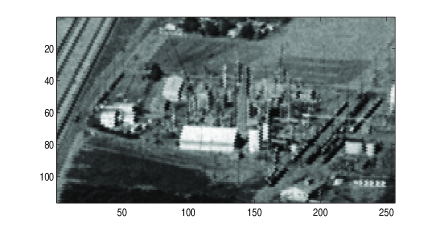
(a) Reference data $X_{5}.$

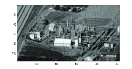
(b) Reference data $X_{18}.$

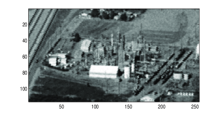
(c) Reference data $X_{31}.$

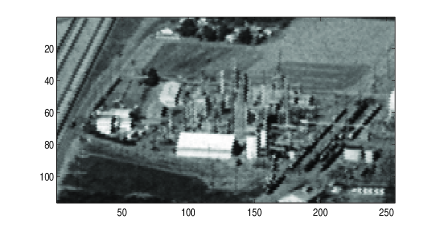
(d) Reference data $X_{44}.$

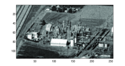
(e) Reference data $X_{57}.$

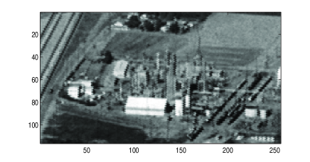
(f) Reference data $X_{70}.$

(g) Reference data $X_{83}.$

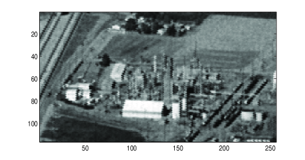
(h) Reference data $X_{96}.$

Figure 1: Examples of reference data from set $K_{{}_{X}}$ to be estimated from observed data.

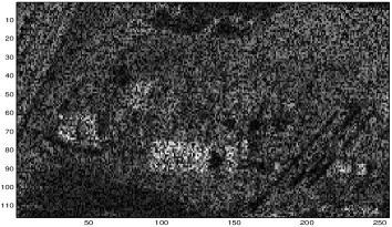
(a) Observed data $Y_{(57)}.$

(b) Observed data $Y_{(70)}.$

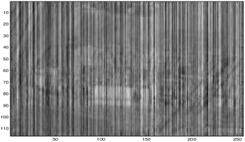
(c) Estimate $\bar{X}_{57}$ by Wiener filter.

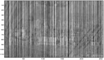
(d) Estimate $\hat{X}_{70}$ by RLS filter.

(e) Estimate $\widetilde{X}_{57}$ by filter $F_{(3)}$.

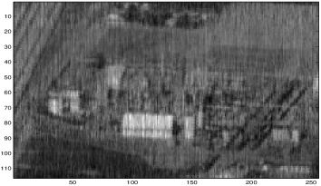
(f) Estimate $\widetilde{X}_{70}$ by filter $F_{(3)}$.

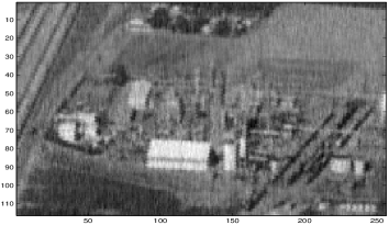
(g) Estimate $\widehat{X}_{57}$ by filter $F_{(5)}$.

(h) Estimate $\widehat{X}_{70}$ by filter $F_{(5)}$.

Figure 2: Illustration to set $K_{{}_{X}}$ estimation by filters $F_{(3)}$ and $F_{(5)}$.

To illustrate Remark 5, i.e., to show that the error $\|\mbox{$\mathbf{x}$}-\mbox{$\mathcal{F}$}_{(p)}(\mbox{$\mathbf{y}$})\|^{2}_{{}_{E}}$ decreases if $p$ increases, an estimate of the set $K_{{}_{X}}=\{X_{1},X_{2},\ldots,X_{100}\}$ has been obtained by the interpolation filter of the $5th$ order $F_{(p)}$, with $p=5$, i.e. with $p$ bigger than $p=3$ considered in (37). In this case, $Q_{j}$, $R_{j}$ and $T_{j}$, for $j=1,\dots,5$ are determined in ways similar to (38)–(39). We denote $\widehat{X}_{i}=F_{(5)}Y_{i}$, for $i=1,\ldots,N$. Estimates $\widehat{X}_{57}$ and $\widehat{X}_{70}$ are given in Fig. 2.

In Table 1, values of the errors $\|X_{i}-F_{(p)}Y_{i}\|^{2}$ are presented for $i=57$ and $i=70$, and $p=3$ and $p=5$.

It follows from Table 1 and Fig. 2 that an increase in $p$ implies a decrease in the error of the estimation.

Note that, although the considered sets $K_{{}_{X}}$ and $K_{{}_{Y}}$ are finite, the above results of their estimation by the interpolation filters can easily be extended to the case when $K_{{}_{X}}$ and $K_{{}_{Y}}$ are infinite. Indeed, if in (35), $\Delta_{i}\rightarrow 0$ as $i\rightarrow\infty$, then $K_{{}_{X}}$ and $K_{{}_{Y}}$ tend to infinite sets. In this case, the choice of sets $S_{{}_{X}}$ and $S_{{}_{Y}}$ can be the same as in (36) above. Then filters $F_{(3)}$ and $F_{(5)}$ will also be the same as above. Therefore, for the case when $K_{{}_{X}}$ and $K_{{}_{Y}}$ are infinite sets, estimates of $K_{{}_{X}}$ by filters $F_{(3)}$ and $F_{(5)}$ are similar to the results obtained above.

3.2 Comparison with Wiener-type filter and RLS filter

In both the Wiener filtering approach and the RLS filtering methodology, a filter should be found for each pair of input-output signals, $\{\mbox{$\mathbf{x}$}_{j},\mbox{$\mathbf{y}$}_{j}\}$ where $j=1,\ldots,100$. That is, in these simulations, $100$ Wiener filters or RLS filters, $\it\Phi_{1},\ldots,\it\Phi_{100}$ or $R_{1},\ldots,R_{100}$, respectively, are required to process signals from $K_{{}_{Y}}$ to $K_{{}_{X}}$. In contrast, our approach requires the single interpolation filter $\mbox{$\mathcal{F}$}_{(p)}$ with $p$ terms (above, we have chosen $p=3$ and $p=5$) where each term requires computational effort that is similar to that required by the single Wiener filter $\it\Phi_{j}$ and the single RLS filter $R_{j}$. Clearly, the Wiener filtering approach and the RLS filtering methodology imply much more computational work [9, 16] to process signals from $K_{{}_{Y}}$ to $K_{{}_{X}}$.

Examples of accuracies associated with the filters $\it\Phi_{57}$ and $R_{70}$ for estimating $X_{57}$ and $X_{70}$ (which represent typical signals under consideration) are given in Table 2, where $\bar{X}_{57}=\it\Phi_{57}(Y_{57})$ and $\hat{X}_{70}=R_{70}(Y_{70})$. The estimates $\bar{X}_{57}$ and $\hat{X}_{70}$ are presented in Fig. 2.

The accuracy associated with the proposed interpolation filter $\mbox{$\mathcal{F}$}_{(p)}$ is better than that of filters $\it\Phi_{j}$ and $R_{j}$ due to the properties of filter $\mathcal{F}$ discussed above (in particular, in Theorems 2 and 3).

4 Conclusion

In this paper, we develop a new approach to filtering of infinite sets of stochastic signals. The approach is based on a filter representation in the form of a sum of $p$ terms. Each term is derived from three matrices, $Q_{i}$, $R_{i}$ and $T_{i}$ with $i=1,\ldots,p$. The methods for determining these matrices have been studied. In particular, matrices $T_{i},\ldots,T_{p}$ are determined from interpolation conditions. This procedure allows us to construct the filter that estimates each signal from the given infinite set with controlled accuracy.

An analysis of the error associated with the filter has been provided. The analysis has shown that the filter has three free parameters with which to improve performance. It follows from the error analysis that the proposed filter is asymptotically optimal. The filter is determined in terms of pseudo-inverse matrices and, therefore, it always exists.

References

• [1] S.T. Alexander and A.L. Ghimikar, A method for recursive least squares filtering based upon an inverse QR decomposition, IEEE Trans. Signal Processing, 41 (1) pp. 20-30, 1993.
• [2] J.A. Apolinario and M.D. Miranda, Convential and Inverse QRD-RLS Algorithms, in QRD-RLS Adaptive Filtering, J.A. Apolinario (Ed), Springer, 2009.
• [3] T. L. Boullion and P. L. Odell, Generalized Inverse Matrices, John Wiley & Sons, Inc., New York, 1972.
• [4] J.H. Ferziger, Numerical Methods for Engineering Applications, Wiley, New-York, 1999.
• [5] V. N. Fomin and M. V. Ruzhansky, Abstract optimal linear filtering, SIAM J. Control Optim., 38, pp. 1334–1352, 2000.
• [6] Y. Gao, M.J. Brennan and P.F. Joseph, A comparison of time delay estimators for the detection of leak noise signals in plastic water distribution pipes, J. Sound and Vibration, Volume 292, Issues 3-5, pp. 552-570, 2006.
• [7] G.H. Golub and C.F. Van Loan, Matrix Computation, Johns Hopkins Univ. Press, 3rd Ed., 1996.
• [8] K. Hayama and M.-K. Fujimoto, Monitoring non-stationary burst-like signals in an interferometric gravitational wave detector, Classical and Quantum Gravity, Issue 8, 2006.
• [9] S. Haykin, Adaptive Filter Theory, 4th Edition, Prentice Hall, Upper Saddle Riever, New Jersey,2002.
• [10] S. Jeona, G. Choa, Y. Huh, S. Jin and J. Park, Determination of a point spread function for a flat-panel X-ray imager and its application in image restoration, in Nuclear Instruments and Methods in Physics Research Section A: Accelerators, Spectrometers, Detectors and Associated Equipment Volume 563, Issue 1, 1 July 2006, pp. 167-171, Proc. of the 7th International Workshop on Radiation Imaging Detectors - IWORID 2005.
• [11] A.N. Kolmogorov and S.V. Fomin, Elements of the Theory of Functions and Functional Analysis, Dover, New York, 1999.
• [12] J. Manton and Y. Hua, Convolutive reduced rank Wiener filtering, Proc. of ICASSP’01, vol. 6, pp. 4001-4004, 2001.
• [13] V. J. Mathews and G. L. Sicuranza, Polynomial Signal Processing, J. Wiley & Sons, 2001.
• [14] L. I. Perlovsky and T. L. Marzetta, Estimating a Covariance Matrix from Incomplete Realizations of a Random Vector, IEEE Trans. on Signal Processing, 40, pp. 2097-2100, 1992.
• [15] G. Robert Redinbo, Decoding Real Block Codes: Activity Detection, Wiener Estimation, IEEE Trans. on Information Theory, vol. 46, No 2, 2000, pp. 609–623.
• [16] A. H. Sayed, Adaptive filters, Hoboken, NJ, Wiley-Interscience, IEEE Press, 2008.
• [17] L.L. Scharf, Statistical Signal Processing: Detection, Estimation, and Time Series Analysis, New York: Addison-Wesley Publishing Co. 1990.
• [18] A. Torokhti and P. Howlett, Method of recurrent best estimators of second degree for optimal filtering of random signals, Signal Processing, 83, 5, pp. 1013 - 1024, 2003.
• [19] A. P. Torokhti, P. G. Howlett and C. Pearce, Optimal recursive estimation of raw data, Annals of Operations Research, 133, pp. 285-302, 2005.
• [20] A. Torokhti and P. Howlett, Optimal transform formed by a combination of nonlinear operators: The case of data dimensionality reduction, IEEE Trans. on Signal Processing, 54, 4, pp. 1431-1444, 2006.
• [21] A. Torokhti and P. Howlett, Computational Methods for Modelling of Nonlinear Systems, Elsevier, 2007.
• [22] A. Torokhti and P. Howlett, Filtering and Compression for Infinite Sets of Stochastic Signals, Signal Processing, 89, pp. 291-304, 2009.
• [23] A.Torokhti and J. Manton, Generic Weighted Filtering of Stochastic Signals, IEEE Transactions on Signal Processing, 57, issue 12, pp. 4675-4685, 2009.
• [24] A. Torokhti and S. Miklavcic, Data compression under constraints of causality and variable finite memory, Signal Processing, 90, issue 10, pp. 2822–2834, 2010.