Quantum computers to test fundamental physics or viceversa

Abstract

We present two complementary viewpoints for combining quantum computers and the foundations of quantum mechanics. On one hand, ideal devices can be used as testbeds for experimental tests of the foundations of quantum mechanics: we provide algorithms for the Peres test of the superposition principle and the Sorkin test of Born’s rule. On the other hand, noisy intermediate-scale quantum (NISQ) devices can be benchmarked using these same tests. These are deep-quantum benchmarks based on the foundations of quantum theory itself. We present test data from Rigetti hardware.

Physics is experimental, so the postulates of all physical theories are based on experiments. Up to now, the role of quantum computers in fundamental physics has mainly been limited to the simulation of complex quantum systems feynman . Here, instead, we propose to use them directly for experimental tests of the postulates of quantum mechanics. In the ideal case, assuming perfect hardware, they are especially suited to this aim as they are quantum systems with a large number of degrees of freedom. In contrast, in the non-ideal case of NISQ devices, one can assume that quantum mechanics is valid and use these tests for fundamentally benchmarking the device, since they are based on the very foundations (the postulates) of the theory. In other words: assuming perfect hardware, one can test quantum mechanics; assuming quantum mechanics, one can test the hardware. Relaxing both assumptions, one can perform self-consistency checks to test both.

We present two such experimental tests: we give algorithms and quantum machine code for the Peres and the Sorkin tests and run them on Rigetti quantum computers. The first one is a test of the state postulate of quantum mechanics (i.e. the superposition principle), which claims that quantum states live in a complex Hilbert space. In principle, one could imagine a quantum mechanics based on real woottersreal ; stu , complex, or quaternionic Hilbert spaces perescompl : the choice is based on the outcome of experiments, such as the Peres one, see also toni ; walther ; greg ; gregor ; janwei ; imagin . The fact that complex numbers are necessary (and sufficient) has interesting implications, e.g. it implies that quantum states are locally discriminable paoloreconstruction and it is connected to the locality of some quantum phenomena toni . The second one, proposed by Sorkin sorkin , is a test of the Born postulate. The Born rule declares that quantum probability is the square modulus of a scalar product in the state space. A failure (or an extension caslav ) of the Born rule would result in a new physical effect: the presence of genuinely $n$-fold superpositions that cannot be reduced to an iteration of the usual two-fold superpositions we find in textbook quantum mechanics caslav ; zykowski ; lee . Thanks to our implementation, we also ran both tests at the same time for a class of states. In contrast to previous tests urbasi ; laflamme ; werner ; walther ; greg , ours do not use custom-built setups, they permit arbitrary initial states, and can be easily scaled up as new reliable quantum computers become available.

There are multiple advantages of doing these (and other) fundamental tests on quantum computers: (i) Both tests are performed on the same hardware, which prevents possible biases that may arise from a tailored experimental setup. At the same time, it is simple to translate the proposed algorithms to different quantum computer architectures, if one wants to confirm the results independently. (ii) It is possible to perform both experiments at the same time (see below), which is important since, as discussed below, the two experiments are not entirely independent of each other. (iii) These experiments are easily scalable to large dimensions, once reliable quantum computers are available. (iv) As discussed one can reverse perspective: under the assumption that quantum mechanics is correct, these tests become deep benchmarks for a quantum computer.

I Peres test

The state postulate claims: “The pure state of a system is described by a normalized vector $|{\psi}\rangle$ in a complex Hilbert space”. As all physical postulates, it is based on experimental data, and the Peres’ test specifically refers to whether one needs complex numbers, reals stu , quaternions perescompl ; zykowski ; adler , octonions lee ; octonions , etc., but it does not question the Hilbert space structure of the theory. For example, we accept the natural assumption that the Hilbert space dimension is equal to the system’s number of degrees of freedom, namely of independent outcomes of a nondegenerate observable (dropping this assumption woottersreal ; stu , one needs different tests for the complexity of quantum mechanics toni ; greg ; walther ; janwei , based on the locality of measurement outcomes). Octonions can be discarded upon observing that they are not associative for multiplication (interestingly, this means that different combinations of two-fold interferences may give different results, which would give the same signature as a failure of the Sorkin test).

We now review the Peres test perescompl . Consider two pure states $\ket{\psi_{1}}$ and $\ket{\psi_{2}}$, and their superpositions $\ket{\psi_{12}}=\alpha\ket{\psi_{1}}+\beta\ket{\psi_{2}}$ with $\alpha,\beta$ nonzero reals. If we project it on, say, $\ket{1}$ (any other state would give similar results), then, assuming complex Hilbert spaces, the probability of successful projection is

$$\left|\braket{1}{\psi_{12}}\right|^{2}= \left|\alpha\braket{1}{\psi_{1}}\right|^{2}+\left|\beta\braket{1}{\psi_{2}}\right|^{2}$$

$$+2\alpha\beta\left|\braket{1}{\psi_{1}}\braket{1}{\psi_{2}}\right|\cos\varphi_{12}$$ (1)

$$\implies\cos\varphi_{12}= \frac{\left|\braket{1}{\psi_{12}}\right|^{2}-\left|\alpha\braket{1}{\psi_{1}}\right|^{2}-\left|\beta\braket{1}{\psi_{2}}\right|^{2}}{2\alpha\beta\left|\braket{1}{\psi_{1}}\braket{1}{\psi_{2}}\right|}$$ (2)

with $\varphi_{12}=\arg(\braket{1}{\psi_{1}}\braket{\psi_{2}}{1})$. If, instead we assume that real Hilbert spaces are sufficient, the term $\cos\varphi_{12}$ can only take the values $\pm 1$. We can rewrite the left-hand-side of (2) in terms of experimental values as

$$\gamma_{12}\coloneqq\frac{p_{12}-\alpha^{2}p_{1}-\beta^{2}p_{2}}{2\alpha\beta\sqrt{p_{1}p_{2}}}$$ (3)

with $p_{12}$, $p_{1}$ and $p_{2}$ the experimental probabilities of projection onto $|1\rangle$ of $|\psi_{12}\rangle$, $|\psi_{1}\rangle$ and $|\psi_{2}\rangle$. If we experimentally find that $\gamma_{12}=\pm 1$ always, then a real quantum theory is sufficient. If we find states for which $|\gamma_{12}|<1$, then it is necessary to use a complex or quaternionic quantum theory. If $|\gamma|>1$, the superposition principle is violated.

To discriminate between a complex and a quaternionic theory we need a further step, based on the identity

$$\cos^{2}a+\cos^{2}b+\cos^{2}c-2\cos a\cos b\cos c=1$$ (4)

valid for any $a,b,c$ real numbers with $a+b+c=0$. Consider three pure states $\ket{\psi_{1}}$, $\ket{\psi_{2}}$, $\ket{\psi_{3}}$, and take superpositions of two at a time. We will have three quantities of the type given in (2) with $\varphi_{12}$, $\varphi_{23},$ or $\varphi_{31}$, one for each pair. Since $\varphi_{12}+\varphi_{23}+\varphi_{31}=0$, then the identity (4) holds for these three angles if a complex quantum theory is sufficient. Otherwise, if a quaternionic theory is necessary, the amplitudes cannot be represented by vectors in a 2D plane and therefore the LHS in (4) is less than 1 in general. One can detect this by analyzing the quantity $F=\gamma_{12}^{2}+\gamma_{23}^{2}+\gamma_{31}^{2}-2\gamma_{12}\gamma_{23}\gamma_{31}$ (where $\gamma_{23},\gamma_{31}$ are defined similarly to $\gamma_{12}$, but using the state $\ket{\psi_{3}}$). If the experimentally measured $F$ is always one for all states, then a complex theory is sufficient (no quaternions, octonions, etc. are needed) since all the $\gamma$s can be written as cosines, and (4) holds. Otherwise if $|F|<1$, then we must employ quarternions. Finally, if $|F|>1$, the superposition principle is violated, as the states cannot be represented as vectors.

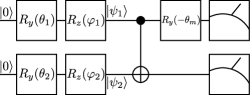
Figure 1: Graphical depiction of the algorithm to calculate the $\gamma$ factor of (7) by creating and projecting superpositions of arbitrary states. The states are created from unitary rotations $R_{\ell}(\lambda)$ of an angle $\lambda$ around the $\ell$ axis, with $a_{k}=\cos\theta_{k}/2$, $b_{k}=\sin\theta_{k}/2$, followed by a CNOT and a rotation by angle $-\theta_{m}$ for desired projection. For example, to project on $\alpha\ket{01}+\beta\ket{10}$, choose $\theta_{m}=2\cos^{-1}\alpha$ and record the counts of $\ket{01}$. The unentangled projections $|\braket{01}{\psi_{1}\psi_{2}}|^{2}$, etc., that are necessary for the $\gamma$s can be measured by a similar circuit where the CNOT-gate and the single-qubit rotation at the end are removed.

The above Peres proposal can be directly implemented on a quantum computer using a unary encoding (one qubit per system) where orthogonal states are mapped into separate physical qubits and their superpositions are obtained through interferences among them, but our tests showed that such procedure is highly sensitive to noise and will be reported elsewhere simanraj . Moreover, one has to make sure that the algorithm does not contain as input the quantity $\cos\varphi_{12}$ of (2), which would render the whole procedure circular. We now present a nontrivial way to overcome both problems: it is suited to current NISQ devices and the cosine term only arises from quantum interference of different paths.

The trick is to prepare a two-qubit factorized state $\ket{\psi_{1}}\ket{\psi_{2}}$ with $\ket{\psi_{k}}=a_{k}\ket{0}+e^{i\varphi_{k}}b_{k}\ket{1}$ ($a_{k}\in[0,1]$, $b_{k}=\sqrt{1-a_{k}^{2}}$), and then project it onto the anti-correlated subspace spanned by $\ket{01}$ and $\ket{10}$. This produces a state proportional to

$$a_{1}b_{2}e^{i\varphi_{2}}\ket{01}+a_{2}b_{1}e^{i\varphi_{1}}\ket{10}\propto a_{1}b_{2}e^{i\varphi_{2}}(\alpha^{*}\ket{\Psi^{+}}+\;$$ (5)

$$\beta\ket{\Psi^{-}})+a_{2}b_{1}e^{i\varphi_{1}}(\beta^{*}\ket{\Psi^{+}}-\alpha\ket{\Psi^{-}}),$$ (6)

$$\mbox{with }\ket{\Psi^{+}}={\alpha\ket{01}+\beta\ket{10}},\ \ket{\Psi^{-}}={\beta^{*}\ket{01}-\alpha^{*}\ket{10}}.$$

By projecting this state onto $\ket{\Psi^{+}}$, we can see the interference among the two $\ket{\Psi^{+}}$ paths present in the state (6). Indeed,

$$2\left|\braket{\Psi^{+}}{\psi_{1}\psi_{2}}\right|^{2}=\left|\alpha\right|^{2}\left|\braket{01}{\psi_{1}\psi_{2}}\right|^{2}+\left|\beta\right|^{2}\left|\braket{10}{\psi_{1}\psi_{2}}\right|^{2}+$$

$$2\mathrm{Re}\left\{\alpha^{*}\beta\right\}\left|\braket{01}{\psi_{1}\psi_{2}}\braket{10}{\psi_{1}\psi_{2}}\right|\cos\varphi_{12}$$ (7)

$$\Rightarrow\cos\varphi_{12}=\tfrac{2\left|\braket{\Psi^{+}}{\psi_{1}\psi_{2}}\right|^{2}-\left|\alpha\right|^{2}\left|\braket{01}{\psi_{1}\psi_{2}}\right|^{2}-\left|\beta\right|^{2}\left|\braket{10}{\psi_{1}\psi_{2}}\right|^{2}}{2\mathrm{Re}\left\{\alpha^{*}\beta\right\}\left|\braket{01}{\psi_{1}\psi_{2}}\braket{10}{\psi_{1}\psi_{2}}\right|}$$

Projections onto an entangled state can be implemented by a CNOT-gate and a single-qubit rotation followed by a measurement in the computational basis. The experimental values of the $\gamma$s can then be obtained by measuring the probability of projection of this state (and of the projection of $\ket{\psi_{1}\psi_{2}}$ onto $\ket{01}$ and $\ket{10}$). The algorithm to create and measure these states is given pictorially in Fig. 1. Once the $\gamma$’s are measured, we can test, by hypothesis testing, whether their experimental values are compatible with $\pm 1$. Similarly for $F$. In principle, the Peres test should check that $F=1$ for all states, which is, of course, not feasible. But, by choosing sets of (uniform) random states, we sample the Hilbert space uniformly.

The experimental results are presented in Fig. 2. The source code of our algorithm using the Rigetti SDK rigettiweb has been uploaded in sourcecode . The fact that a complex quantum theory is necessary, and it is also sufficient as quaternions are not required, is confirmed by our results up to experimental error (which we fully characterized). All the circuits are run for $10^{4}$ shots and the limited sample gives rise to significant statistical fluctuations in the results, indicated in the plots by 3$\sigma$ confidence intervals. We also plotted the values obtained from simulations on Rigetti’s Quantum Virtual Machine (QVM). Because of noises in the quantum computer, the result of the Peres-test has significant deviations from the theoretical values. However, when we take into account the dominant errors (readout and dephasing errors here) in the gates in a noisy simulation, we observe similar deviations in the results. The samples collected from the quantum computer and the noisy simulator are also bootstrapped to find a confidence interval based on that sample. This confirms that the observed value of $F<1$ is due to the noises, and we cannot reject the hypothesis that complex numbers are sufficient. We explore the effects of different types of errors in simanraj .

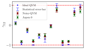
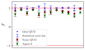
Figure 2: Plots of the $\gamma_{12}$ and of $F$ for different sets of (uniformly distributed) random states. The green circles are the measured outputs on Rigetti Aspen-9 device, the blue stars are the (ideal) quantum prediction from Rigetti’s quantum virtual machine (QVM), the red squares are the quantum prediction that takes into account the systematic noise sources (the noise parameters are obtained from Rigetti’s own calibration data). Most $\gamma$ values are different from $\pm 1$, which implies that a real Hilbert space is insufficient. The values of $F$ are all smaller than one, but they are all statistically compatible with the value corrected by taking into account the readout and dephasing errors in the hardware (the green and red error bars overlap). Thus, the $F$ data should be considered as a deep-quantum benchmark for the hardware. No quantities are outside the interval $[-1,1]$, so the superposition principle is not violated.

II Sorkin test

The measurement postulate (Born rule) claims: “The probability that a measurement of a property $O$, described by the operator with spectral decomposition $\sum_{j}o_{j}\ket{j}\bra{j}$, returns a value $o_{j}$, given that the system is in state $\ket{\psi}$, is $p(o_{j}|\psi)={|\braket{\psi}{j}|^{2}=|x_{j}|^{2}}$, with $\ket{\psi}=\sum_{j}x_{j}\ket{j}$” .

The linearity of quantum mechanics implies that, if a value $o_{j}$ of some system property is determined by two or more indistinguishable pathways, the probability of measuring such value is obtained from the sum (interference) of the amplitudes for each (superposition principle). This interference is encoded in the postulate by the scalar product $\braket{\psi}{j}$ (whose definition contains a sum). The exponent 2 in the probability postulate implies that the superposition of more than two pathways gives the same probability that is obtained by separately considering the interference of all the couples of paths independently sorkin ; caslav . Namely no genuinely $n$-path interference effects appear for $n>2$. In fact, for $n=3$, assuming the Born rule, consider the following probabilities

$$p_{123}=\left|\left(\frac{\bra{1}+\bra{2}+\bra{3}}{\sqrt{3}}\right)\ket{\psi}\right|^{2}=\frac{\left|x_{1}+x_{2}+x_{3}\right|^{2}}{3}$$ (8)

$$p_{12}=\left|\left(\frac{\bra{1}+\bra{2}}{\sqrt{2}}\right)\ket{\psi}\right|^{2}=\frac{\left|x_{1}+x_{2}\right|^{2}}{2},\mbox{ etc.}$$ (9)

$$p_{1}=\left|\braket{1}{\psi}\right|^{2}=\left|x_{1}\right|^{2},\mbox{ etc.},$$ (10)

where the bras refer to the $O$ eigenstates $\ket{j}$, and the term (8) refers to a three-path interference, (9) to two-path interference and (10) is the probability of each path by itself. The exponent 2 ensures that the multipath probability can always be expressed in terms of the two-path and single-path ones. Indeed the quantity

$$\kappa_{3}=3p_{123}-2(p_{12}+p_{23}+p_{13})+p_{1}+p_{2}+p_{3}\;$$ (11)

is identically null thanks to the following identity, valid for any three complex numbers $x_{1},x_{2},x_{3}$:

$$3\left|\tfrac{x_{1}+x_{2}+x_{3}}{\sqrt{3}}\right|^{2}-2\Big{[}\left|\tfrac{x_{1}+x_{2}}{\sqrt{2}}\right|^{2}+\left|\tfrac{x_{1}+x_{3}}{\sqrt{2}}\right|^{2}+\left|\tfrac{x_{2}+x_{3}}{\sqrt{2}}\right|^{2}\Big{]}$$

$$+\left|x_{1}\right|^{2}+\left|x_{2}\right|^{2}+\left|x_{3}\right|^{2}=0.$$ (12)

Sorkin sorkin proposed to check the form of the Born rule and the superposition principle by measuring the probabilities (8)-(10) and calculating the experimental value of $\kappa_{3}$ to check if it is null (up to statistical errors). This can be extended to arbitrary $n$. In fact, if we assume (or measure experimentally) that the $\kappa_{j}$’s up to $j=n-1$ are null, one can show by induction that

$$\kappa_{n}= \Big{|}\sum\limits_{j=1}^{n}x_{j}\Big{|}^{2}-\sum\limits_{j,k>j}^{n-1,n}|x_{j}+x_{k}|^{2}+(n-2)\sum\limits_{j=1}^{n}|x_{j}|^{2},$$ (13)

so that one can incrementally increase $n$ by just measuring the $n$-path, the $2$-path and $1$-path probabilities.

Importantly, one has to ensure that the pathways are distinguishable (i.e. they are described by orthogonal states), otherwise interferences are not obtained through simple sums as in (8)-(10). Initial experiments were carried out following Sorkin’s proposal of multi-slit experiments urbasi which are only approximately orthogonal (looping paths that go through multiple slits exist urbasi2 ; rengaraj ; usinha3 ). As we do here, some tests used orthogonal states gsch , where a null result is easier to evaluate.

To implement Sorkin’s test on a quantum computer we need to create an arbitrary superposition of $n$ orthogonal pathways. This can be done using $n$ qubits with a unary encoding simanraj or, more efficiently and in a less error-prone manner with $\log_{2}n$ qubits in a binary encoding. Start with $n=3$: the circuit to create arbitrary three level states with binary encoding is presented in Fig. 3a. It implements the transformation $U(\theta_{1},\varphi_{1},\theta_{2},\varphi_{2})|00\rangle$ which prepares the state

$$\ket{\psi}=\cos\tfrac{\theta_{1}}{2}e^{-i\varphi_{1}/2}\ket{00}+\sin\tfrac{\theta_{1}}{2}e^{i\varphi_{1}/2}\cos\tfrac{\theta_{2}}{2}e^{-i\varphi_{2}/2}\ket{10}$$

$$+\sin\tfrac{\theta_{1}}{2}e^{i\varphi_{1}/2}\sin\tfrac{\theta_{2}}{2}e^{i\varphi_{2}/2}\ket{11},$$ (14)

where $\theta_{k}$ and $\varphi_{k}$ are defined in the figure caption and are chosen randomly. To get the probabilities (8)-(10), we need to project $|\psi\rangle$ onto a state $\langle\psi^{\prime}|$ such as $\left(\bra{00}+\bra{10}+\bra{11}\right)/\sqrt{3}$, etc. The state $\bra{\psi^{\prime}}=\bra{00}U^{\dagger}(t_{1},f_{1},t_{2},f_{2})$ is implemented by the adjoint of the circuit of Fig. 3a with appropriate $t_{1},f_{1},t_{2},f_{2}$, and the projection is $\braket{00}{U^{\dagger}(t_{1},f_{1},t_{2},f_{2})U(\theta_{1},\varphi_{1},\theta_{2},\varphi_{2})}{00}$. The simplified quantum circuit to implement $U^{\dagger}(t_{1},0,t_{2},0)U(\theta_{1},\varphi_{1},\theta_{2},\varphi_{2})$ is shown in Fig. 3b. Measurements in the computational basis can be done by setting $t_{1}=t_{2}=0$ and getting all the projections from the same run of the circuit. Using this circuit, we performed the three-level Sorkin test on a number of randomly chosen states. The results are presented in Fig. 4 and they confirm that $\kappa_{3}$ is statistically compatible with zero, as expected.

The extension to arbitrary $n$ can be obtained from the measurement of the $n$-path probability: it can be implemented using a Hadamard gate on each path followed by computational basis measurement if $n$ is a power of two or, in general, from a circuit whose adjoint creates a uniform superposition starting from a $\ket{0\cdots 0}$ state. The probability of obtaining all zeros from this measurement gives the first term of the hierarchy, namely the first sum in (13), i.e. Eq. (8) for $n=3$. Then we only require 2-path and 1-path probabilities that can be obtained with a trivial extension of the above procedure: translate to binary and use two-qubit correlations for the 2-path probabilities or measure the computational basis for the 1-path probabilities. This is sufficient, in principle, to incrementally scale the Sorkin test to large $n=2^{N}$ using $N$ qubits simanraj , although in practice, current NISQ device limitations prevent us from testing for large $n$ as errors increase with increasing number of qubits.

(a)

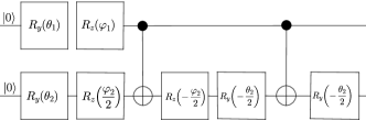
(b)

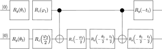
Figure 3: Sorkin test circuits. (a) Circuit to prepare arbitrary three-level states (II): $R_{\ell}(\lambda)$ represents a rotation around the $\ell$ axis by an angle $\lambda$. (b) Complete circuit that includes also the measurements. The parameters ${t}_{1}$ and ${t}_{2}$ are used to select the different measurements. For example, the projection onto $|00\rangle+|10\rangle+|11\rangle$ discussed in the text is obtained by choosing ${t}_{1}=2\cos^{-1}\left(1/\sqrt{3}\right)$, ${t}_{2}=2\cos^{-1}\left(1/\sqrt{2}\right)$.

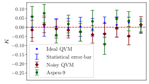
Figure 4: Plot of $\kappa_{3}$ of Eq. (11) of the Sorkin test for randomly chosen states performed using the circuit of Fig. 3b. All obtained values are compatible with the theoretical value $\kappa_{3}=0$ expected from standard quantum mechanics. The error bars are produced using the same method as in the case of Peres’ test above.

Interestingly, our algorithmic procedure allows us to perform the Peres and Sorkin tests jointly for a class of states. Instead of using the above procedure to prepare the Sorkin test state, we use the Peres test circuit of Fig. 1 to produce and project a set of randomly generated states of the form $\ket{\psi_{1}\psi_{2}}=a\ket{00}+b\ket{01}+c\ket{10}+d\ket{11}$. We then consider the projections onto $\ket{00}+\ket{01}+\ket{10}$, onto the two path-states $\ket{00}+\ket{01}$, $\ket{00}+\ket{10}$ and $\ket{01}+\ket{10}$ and onto the singles. For Sorkin test, we make an additional projection on $\ket{00}+\ket{01}+\ket{10}$ by replacing the CNOT and single qubit rotation at the end with the adjoint of the circuit that transforms $\ket{00}\rightarrow\left(\ket{00}+\ket{01}+\ket{10}\right)/\sqrt{3}$ and then measuring $\ket{00}$. Since the state $\ket{11}$ never appears in these measurements, this procedure is equivalent to first projecting the state $\ket{\psi_{1}\psi_{2}}$ onto the subspace spanned by $\ket{00}$, $\ket{01}$ and $\ket{10}$ and then performing the Sorkin test on the projected state (Results in Fig. 5).

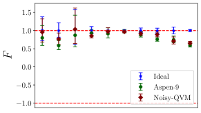
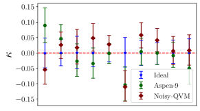
Figure 5: Results of Peres’ and Sorkin’s test using the same set of states and circuits for both. The data acquired to perform Sorkin’s test in this case were sufficient to perform Peres’ test and therefore, the same data-set is used to plot both $\kappa_{3}$ and $F$. The results of the joint Peres-Sorkin test are consistent with theoretical expectations, taking into account the readout and dephasing errors present in the system. These results are also consistent with the results of the standalone versions of the Peres’ and Sorkin’s test shown above (the values are, however, different because the set of random states used in each case is different).

III Conclusions

We propose and implement quantum algorithms to test some of the physical principles behind two postulates of quantum mechanics: the complex nature of quantum Hilbert spaces and the form of the Born rule. We also perform both tests at the same time. We present results on a NISQ device that can be interpreted as a deep quantum benchmark of such devices. We initially believed that we could translate the Peres and Sorkin tests into quantum algorithms in a straightforward manner, but we found we had to modify these tests in a nontrivial way both due to the practical limitations of current NISQ devices and to the fundamental limitations of the gate model of quantum computation, which would require, as an input to the un-modified Peres algorithm, the same quantity $\gamma$ that one then measures simanraj .

IV Acknowledgments

LM acknowledges funding from the MIUR Dipartimenti di Eccellenza 2018-2022 project F11I18000680001 and from the U.S. Department of Energy, Office of Science, National Quantum Information Science Research Centers, Superconducting Quantum Materials and Systems Center (SQMS). We acknowledge support from Rigetti, and in particular from Matt Reagor. US acknowledges partial support provided by the Ministry of Electronics and Information Technology (MeitY), Government of India under grant for Centre for Excellence in Quantum Technologies with Ref. No. 4(7)/2020 - ITEA, QuEST-DST project Q-97 of the Govt. of India and the QuEST-ISRO research grant.

References

- (1) R. P. Feynman, Simulating Physics with Computers, Int. J. Theor. Phys. 21, 467 (1982).
- (2) W.K. Wootters, Optimal Information Transfer and Real-Vector-Space Quantum Theory. In: Chiribella G., Spekkens R. (eds) Quantum Theory: Informational Foundations and Foils. Fundamental Theories of Physics, vol 181. Springer (2016), arXiv:1301.2018.
- (3) E.C.G. Stueckelberg, Quantum Theory in Real Hilbert Space, Helv. Phys. Acta 33, 727 (1960).
- (4) A. Peres, Proposed Test for Complex versus Quaternion Quantum Theory, Phys. Rev. Lett. 42, 683 (1979).
- (5) M.-O. Renou, D. Trillo, M. Weilenmann, L.P. Thinh, A. Tavakoli, N. Gisin, A. Acin, M. Navascues, Quantum physics needs complex numbers, arXiv:2101.10873 (2021).
- (6) L.M. Procopio, L.A. Rozema, Z.J. Wong, D.R. Hamel, K. O’Brien, X. Zhang, B. Dakic, P. Walther, Single-photon test of hyper-complex quantum theories using a metamaterial, Nature Comm. 8 15044 (2017).
- (7) R. Keil, T. Kaufmann, T. Kauten, S. Gstir, C. Dittel, R. Heilmann, A. Szameit, G. Weihs, Hybrid waveguide-bulk multi-path interferometer with switchable amplitude and phase, APL Phot. 1, 081302 (2016).
- (8) S. Gstir, E. Chan, T. Eichelkraut, A. Szameit, R. Keil, G. Weihs, Towards probing for hypercomplex quantum mechanics in a waveguide interferometer, New. J. Phys. to be published, arXiv:2104.11577 (2021).
- (9) M.-C. Chen, et al., Ruling out real-number description of quantum mechanics, arXiv:2103.08123 (2021).
- (10) K.-D. Wu, T. Varun Kondra, S. Rana, C. M. Scandolo, G.-Y. Xiang, C.-F. Li, G.-C. Guo A. Streltsov, Operational Resource Theory of Imaginarity, Phys. Rev. Lett. 126, 090401 (2021).
- (11) G. Chiribella, G.M. D’Ariano, P. Perinotti, Informational derivation of quantum theory, Phys. Rev. A 84, 012311 (2011).
- (12) R.D. Sorkin, Quantum Mechanics as Quantum Measure Theory, Mod. Phys. Lett. A 9, 3119 (1994).
- (13) B. Daki, T. Paterek, C. Brukner, Density cubes and higher-order interference theories, New J. Phys. 16(2), 023028 (2014).
- (14) K. Zyczkowski, Quartic quantum theory: an extension of the standard quantum mechanics, J. Phys. A 41, 355302 (2008).
- (15) C.M. Lee, J.H. Selby, Higher-Order Interference in Extensions of Quantum Theory, Found. Phys. 47,
- (16) U. Sinha, C. Couteau, T. Jennewein, R. Laflamme, G. Weihs, Ruling out multi-order interference in quantum mechanics, Science 329, 418 (2010).
- (17) D. K. Park, O. Moussa, R. Laflamme, Three path interference using nuclear magnetic resonance: a test of the consistency of Born’s rule, New J. Phys. 14, 113025 (2012).
- (18) H. Kaiser, E. A. George, S. A. Werner, Neutron interferometric search for quaternions in quantum mechanics, Phys. Rev. A 29, 2276(R) (1984).
- (19) S. L. Adler, Generalized quantum dynamics, Nucl. Phys. B 415, 195 (1994).
- (20) S. De Leo, K. Abdel-Khalek, Octionionic Quantum Mechanics and Complex Geometry, Prog. Theor. Phys. 96, 823 (1996).
- (21) S. Sadana, L. Maccone, U. Sinha, Quantum Computational tests of the Born Rule, in preparation.
- (22) Rigetti SDK at https://qcs.rigetti.com/sdk-downloads.
- (23) http://www.rri.res.in/QuicLab/Peres_Sorkin/
- (24) R. Sawant, J. Samuel, A. Sinha, S. Sinha, U. Sinha, Nonclassical Paths in Quantum Interference Experiments, Phys. Rev. Lett. 113, 120406 (2014).
- (25) G. Rengaraj, U. Prathwiraj, S. N. Sahoo, R. Somashekhar, U. Sinha, New J. Phys. 20, 063049 (2018).
- (26) A. Sinha, A. H. Vijay, U. Sinha, Scientific Reports, 5, 1–9 (2015).
- (27) I. Söllner, B. Gschösser, P. Mai, B. Pressl, Z. Vörös, G. Weihs, Testing Born’s rule in quantum mechanics for three mutually exclusive events, Found. Phys. 42, 742 (2012).
- (28) G. Lüders, Über die Zustandsänderung durch den Messprozess, Ann. Phys., Lpz. 8, 322 (1951).