TAP equations are repulsive.

Abstract.

We show that for low enough temperatures, but still above the AT line, the Jacobian of the TAP equations for the SK model has a macroscopic fraction of eigenvalues outside the unit interval. This provides a simple explanation for the numerical instability of the fixed points, which thus occurs already in high temperature. The insight leads to some algorithmic considerations on the low temperature regime, also briefly discussed.

1. Introduction

Let $N\in\mathbb{N},\beta>0,h\in\mathbb{R}$, and consider independent standard Gaussians $\bm{g}=(g_{ij})_{1\leq i<j\leq N}$ issued on some probability space $(\Omega,\mathcal{F},\mathbb{P})$. The TAP equations [18, after Thouless, Anderson and Palmer] for the spin magnetizations $\bm{m}=(m_{i})_{i=1}^{N}\in[-1,1]^{N}$ in the SK-model [11, after Sherrington and Kirkpatrick] at inverse temperature $\beta$ and external field $h$ read

$$m_{i}=\tanh\left(h+\frac{\beta}{\sqrt{N}}\sum_{j:j\neq i}g_{ij}m_{j}-\beta^{2}(1-q)m_{i}\right),\quad i=1,\ldots,N.$$ (1.1)

The $\beta^{2}$-term is the (limiting) Onsager correction: it involves the high temperature order parameter $q$ which is the (for $\beta\leq 1$ or $h\neq 0$ unique, see [12, Proposition 1.3.8]) solution of the fixed point equation

$$q=\mathbb{{\sf{E}}}\tanh^{2}\left(h+\beta\sqrt{q}Z\right),$$ (1.2)

$Z$ being a standard Gaussian, and ${\sf{E}}$ its expectation.

The concept of high temperature is related to the AT-line [2, after de Almeida and Thouless], i.e. the $(\beta,h)$-region satisfying

$$\beta^{2}{\sf{E}}\frac{1}{\cosh^{4}(h+\beta\sqrt{q}Z)}=1.$$ (1.3)

For $(\beta,h)$ where the l.h.s. is strictly less than unity, the system is allegedly in the replica symmetric phase (high temperature), see e.g. Adhikari et.al. [1] for a recent thorough discussion of this issue, and Chen [9] for evidence supporting the conjecture.

Due to the fixed point nature of the TAP equations (1.2), one is perhaps tempted to solve them numerically via classical Banach iterations, i.e. to approximate solutions via

$$m_{i}^{(k+1)}=\tanh\left(h+\frac{\beta}{\sqrt{N}}\sum_{j:j\neq i}g_{ij}m_{j}^{(k)}-\beta^{2}(1-q)m_{i}^{(k)}\right),\quad i=1,\ldots,N,$$ (1.4)

As it turns out, these plain iterations are astonishingly in-efficient in finding stable fixed points insofar the mean squared error between two iterates, to wit:

$$\text{MSE}\left(\bm{m}^{(k+1)},\bm{m}^{(k)}\right)\equiv\frac{1}{N}\sum_{i=1}^{N}\left(m_{i}^{(k+1)}-m_{i}^{(k)}\right)^{2},$$ (1.5)

often remains large, even for very large $k^{\prime}s$. Even more surprising, this issue is not restricted to the low temperature phase, cfr. Figure 1 below.

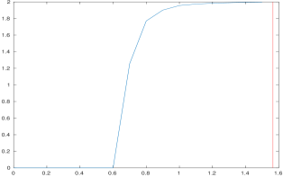
Figure 1. MSE between (the last) two iterates as a function of $\beta$, to fixed magnetic field $h=0.5$, a single realization of the disorder, and system size $N=25$. We have run Banach algorithm $k=1000$ times, randomly initialized (uniformly chosen $\bm{m}^{(0)}$). Visibly, iterations stabilize for small $\beta$, but diverge beyond the threshold $\approx 0.6$, way below the AT-line (red).

Bolthausen [6] bypasses this problem by means of a modification of the Banach algorithm (recalled below) which converges up to the AT-line. Notwithstanding, the origin of the phenomenon captured by Figure 1 has not yet been, to our knowledge, identified. It is the purpose of this work to fill this gap. Precisely, we show in Theorem 1 below that classical Banach iterates become unstable for the simplest reason: for large enough $\beta$, but still below the AT-line, TAP equations become repulsive. This should be contrasted with the classical counterpart of the SK-model: it is well known (and a simple fact) that relevant solutions of the fixed point equations for the Curie-Weiss model are attractive at any temperature, with the irrelevant solution even becoming repulsive in low temperature.

2. Main result

2.1. Iterative procedure for the magnetizations

Bolthausen [6] constructs magnetizations ${\bm{m}}^{(k)}=\left(m^{(k)}_{i}\right)_{i\leq N}$ for given disorder $(g_{ij})_{1\leq i<j\leq N}$ through an iterative procedure in $k=1,2,\dots$. These magnetizations approximate fixed points of the TAP equations in the limit $N\to\infty$ followed by $k\to\infty$. The algorithm uses the initial values ${\bm{m}}^{(0)}=\bm{0}$, ${\bm{m}}^{(1)}=\sqrt{q}\bm{1}$. The iteration step reads

$$m^{(k+1)}_{i}=\tanh\left(h+\frac{\beta}{\sqrt{N}}\sum_{j:\>j\neq i}g_{ij}m^{(k)}_{j}-\beta^{2}(1-q)m^{(k-1)}_{i}\right),$$ (2.1)

for $i\leq N$, and $k\in\mathbb{N}$. Remark in particular that contrary to the classical Banach algorithm, the above scheme invokes a time delay in the Onsager correction: we will thus refer to (2.1) as Two Steps Banach algorithm, 2SteB for short. By [6, Proposition 2.5], the quantity $q_{N}:=N^{-1}\sum_{i=1}^{N}(m^{(k)}_{i})^{2}$ converges to $q$ in probability and in expectation, as $N\to\infty$ followed by $k\to\infty$. Moreover, by [6, Theorem 2.1],

$$\lim_{k,k^{\prime}\to\infty}\limsup_{N\to\infty}\mathbb{E}\left[\frac{1}{N}\sum_{i=1}^{N}\left(m^{(k)}_{i}-m^{(k^{\prime})}_{i}\right)^{2}\right]=0,$$ (2.2)

provided $(\beta,h)$ is below the AT-line, i.e. if the left-hand side of (1.3) is less than unity.

2.2. Spectrum of the Jacobian

Denote by $F_{i}(\bm{m}^{(k)})$ the right-hand side of (1.4), and consider the Jacobi matrix $J^{(k)}$ with entries

$$J^{(k)}_{ij}:=\frac{\partial F_{i}}{\partial m_{j}}({\bm{m}}^{(k)})=\begin{cases}\frac{\beta}{\sqrt{N}}g_{ij}\left(1-F_{i}\left({\bm{m}}^{(k)}\right)^{2}\right):i\neq j\\ -\beta^{2}(1-q)\left(1-F_{i}\left({\bm{m}}^{(k)}\right)^{2}\right):i=j,\end{cases}$$ (2.3)

omitting the obvious $N$-dependence to lighten notations.

The Jacobi matrix $J^{(k)}$ is not symmetric, but we claim that it is nonetheless diagonalizable, and that all eigenvalues are real. To see this we write the Jacobian as a product

$$J^{(k)}=\hat{J}{\rm diag}\left(1-F_{\cdot}\left({\bm{m}}^{(k)}\right)^{2}\right),$$ (2.4)

where

$$\hat{J}_{ij}:=\begin{cases}\frac{\beta}{\sqrt{N}}g_{ij}&i<j,\\ \frac{\beta}{\sqrt{N}}g_{ji}&j<i,\\ -\beta^{2}(1-q)&i=j.\end{cases}$$ (2.5)

The first matrix on the r.h.s. of (2.4) is symmetric, whereas the second is negative definite: it thus readily follows from [10, Theorem 2] that $J^{(k)}$ itself is diagonalizable, and that all its eigenvalues are real, settling our claim.

Denoting the ordered sequence of the real eigenvalues of a matrix $M$ by $\lambda_{1}(M)\geq\ldots\geq\lambda_{N}(M)$, we then consider the empirical spectral measure of the Jacobian

$$\mu^{(k)}:=\frac{1}{N}\sum_{i=1}^{N}\delta_{\lambda_{i}(J^{(k)})}.$$ (2.6)

Our main result states that in a region below the AT-line, $\mu^{(k)}$ has mass outside the unit interval.

Theorem 1.

For all $\beta\in(\sqrt{2}-1,1)$ and $\epsilon>0$, there exists $h_{0}>0$ such that the following holds true: for all $h\in[0,h_{0}]$, there exists $k_{0}\in\mathbb{N}$, and for all $k\geq k_{0}$, there exists $N_{0}\in\mathbb{N}$, such that $\mathbb{P}\left(\mu^{(k)}(-\infty,-1)>0\right)\geq 1-\epsilon$, for all $N\geq N_{0}$.

TAP equations thus become repulsive due a macroscopic fraction of low-lying ($<-1$) eigenvalues. Before giving a proof of this statement, we remark that the measures $\mu^{(k)}$ converge to a limiting measure $\mu$ which can be stated as a free multiplicative convolution

$$\mu=\lambda_{\beta,q}\boxtimes\nu,$$ (2.7)

where $\lambda_{\beta,q}$ is the law of $\beta X-\beta^{2}(1-q)$ for $X$ distributed according to the standard semicircular law with density $x\ni[-2,2]\mapsto(2\pi)^{-1}\sqrt{(4-x^{2}}$, and $\nu$ is the law of $1-\tanh^{2}(h+\beta\sqrt{q}Z)$ for $Z$ standard Gaussian. To sketch a proof of this claim, we use the decomposition (2.4) and make the following observations: i) The empirical spectral distribution of the first factor $\hat{J}$ weakly-converges almost surely to the scaled/shifted semicircular law $\lambda_{\beta,q}$; ii) The empirical spectral distribution of the second factor $1-F_{\cdot}({\bm{m}}^{(k)})^{2}$ can similarly be shown to converge to $\nu$. These observations, together with the (asymptotic) independence of the two factors which follows from [7], and finally [4, Theorem 5.4.2] then yield the representation (2.7).

The free convolution can also be evaluated more explicitly using Voiculescu’s S-transform via inversion of moment generating functions, see e.g. [4, Chapter 5.3]. We believe this approach allows to remove the small-$h$ condition in Theorem 1. The ensuing analysis is however both long and (tediously) technical. As the outcome arguably adds little to the main observation of this work, we refrain from pursuing this route here.

Proof of Theorem 1.

In a first step we consider a simplified version of the Jacobian, namely the matrix $\hat{J}$ from (2.5) in place of $J^{(k)}$. We write $\hat{J}=W-\beta^{2}(1-q)I$, where $W$ is a Wigner matrix. As a consequence of Wigner’s theorem, see e.g. [17, Theorem 2.4.2], the empirical spectral measure $\hat{\mu}$ associated with $\hat{J}$ converges a.s. with respect to the vague topology to the law of $\beta X-\beta^{2}(1-q)$, where $X$ has the standard semicircular density. We note that this limit law has mass in any right vicinity of $-2\beta-\beta^{2}(1-q)$.

Next we show that $\mu^{(k)}$ and $\hat{\mu}$ converge to the same limit as $N\to\infty$ followed by $k\to\infty$, and finally $h\to 0$. To this aim, let $R^{(k)}(z)=(J^{(k)}-zI)^{-1}$ and $\hat{R}(z)=(\hat{J}-zI)^{-1}$ denote the resolvents of $J^{(k)}$ and $\hat{J}$, respectively. It suffices to show that the Stieltjes transforms $N^{-1}{\rm tr}\,\hat{R}(z)$ and $N^{-1}{\rm tr}\,R^{(k)}(z)$ of $\hat{\mu}$ and $\mu^{(k)}$, respectively, converge to the same limit in probability as $N\to\infty$ followed by $k\to\infty$ and $h\to 0$, pointwise for all $z\in\mathbb{C}$ with $\Im z>0$ (see e.g. [17, Section 2.4.3] for properties of the Stieltjes transform). By the resolvent identity,

$$N^{-1}{\rm tr}\,R^{(k)}(z)-N^{-1}{\rm tr}\,\hat{R}(z)=N^{-1}{\rm tr}\,R^{(k)}(z)\left(\hat{J}-J^{(k)}\right)\hat{R}(z).$$ (2.8)

The $p$-Schatten norm of an $N\times N$ matrix $M$ whose eigenvalues are all real is defined by

$$\|M\|_{p}:=\left(\sum_{i=1}^{N}|\lambda_{i}(M)|^{p}\right)^{1/p}\text{ for }p\in[1,\infty),\quad\|M\|_{\infty}:=\max\left\{\left|\lambda_{i}(M)\right|:i=1,\ldots,N\right\}$$ (2.9)

which satisfies $\|M\|_{1}\geq|{\rm tr}\,M|$ and the Hölder inequality. Hence, the expression in (2.8) is bounded in absolute value by

$$\|R^{(k)}(z)\|_{\infty}\|\hat{R}(z)\|_{\infty}\|\hat{J}\|_{\infty}N^{-1}\|{\rm diag}F_{\cdot}({\bm{m}}^{(k)})^{2}\|_{1},$$ (2.10)

where we evaluated $\hat{J}-J^{(k)}$ using (2.4). Each of the first two terms in (2.10) is bounded by $1/|\Im z|$, which follows from the definition of the resolvent. The third term $\|\hat{J}\|_{\infty}$ converges in probability to $2\beta+\beta^{2}(1-q)$ as $N\to\infty$ by Wigner’s theorem in conjunction with edge scaling for Wigner matrices, see e.g. [4, Chapter 3], and [3] for a recent reference. From the definitions of $F_{i}(\bm{m}^{(k)})$ and $m^{(k+1)}_{i}$, and as the function $x\mapsto\tanh^{2}(x)$ is 2-Lipschitz continuous, we obtain

$$\left|F_{i}(\bm{m}^{(k)})^{2}-{m^{(k+1)}_{i}}^{2}\right|=\bigg{|}\tanh^{2}\left(h+\frac{\beta}{\sqrt{N}}\sum_{j:j\neq i}g_{ij}m^{(k)}_{j}-\beta^{2}(1-q)m^{(k)}_{i}\right)\\ -\tanh^{2}\left(h+\frac{\beta}{\sqrt{N}}\sum_{j:j\neq i}g_{ij}m^{(k)}_{j}-\beta^{2}(1-q)m^{(k-1)}_{i}\right)\bigg{|}\leq 2\beta^{2}(1-q)\left|m^{(k)}_{i}-m^{(k-1)}_{i}\right|.$$ (2.11)

Hence, by definition of the $1$-Schatten norm,

$$N^{-1}\|{\rm diag}F_{\cdot}({\bm{m}}^{(k)})^{2}\|_{1}\leq N^{-1}\sum_{i=1}^{N}\left(m^{(k)}_{i}\right)^{2}+2N^{-1}\sum_{i=1}^{N}\left|1\cdot\left(m^{(k)}_{i}-m^{(k-1)}_{i}\right)\right|.$$ (2.12)

The second term on the r.h.s. is bounded by

$$2N^{-1/2}\left[\sum_{i=1}^{N}\left(m^{(k)}_{i}-m^{(k-1)}_{i}\right)^{2}\right]^{1/2}$$ (2.13)

by the Cauchy-Schwarz inequality and thus converges to $0$ in probability as $N\to\infty$ followed by $k\to\infty$ by (2.2). The first term on the r.h.s. of (2.12) equals $q_{N}$ and thus converges to $q$ in probability as $N\to\infty$ followed by $k\to\infty$. From (1.2), we obtain

$$q=\mathbb{{\sf{E}}}\tanh^{2}\left(h+\beta\sqrt{q}Z\right)\leq h^{2}+\beta^{2}q\,,$$ (2.14)

and

$$0\leq q\leq\frac{h^{2}}{1-\beta^{2}}\,,$$ (2.15)

for $\beta\in(0,1)$, hence $h\to 0$ implies $q\to 0$.

From the above, it follows that $\mu^{(k)}$ and $\hat{\mu}$ converge in probability to the same vague limit $\mu$ as $N\to\infty$ followed by $k\to\infty$ and $h\to 0$. For $h=0$ and $\beta\in(\sqrt{2}-1,1)$, we have $\mu(-\infty,-1)>0$ a.s. as a consequence of the first part of the proof. The assertion now follows from the vague convergence in probability of $\mu^{(k)}$ to $\mu$. ∎

3. Yet another algorithm, and simulations

The above considerations pertain to high temperature, but naturally lead to insights into the low temperature regime, where finding solutions of the TAP equations is notoriously hard. Indeed, Theorem 1 suggests that the numerical instability of classical iteration schemes is “nothing structural”, but heavily depends on the way TAP equations are written. Under this light, the following iteration scheme, which we refer to as $\varepsilon$-Banach, is quite natural: for $\varepsilon\in\mathbb{R}$ an additional free parameter, it reads

$$m^{(k+1)}_{i}=\varepsilon m^{(k)}+(1-\varepsilon)\tanh\left(h+\frac{\beta}{\sqrt{N}}\sum_{j:\>j\neq i}g_{ij}m^{(k)}_{j}-\beta^{2}(1-q_{N})m^{(k)}_{i}\right),$$ (3.1)

for $i=1\dots N,k\in\mathbb{N}$. The idea behind the “$\varepsilon$-splitting” is of course to mitigate the impact of large negative Jacobian-eigenvalues. We emphasize that:

• Here and henceforth we consider the finite-$N$ Onsager reaction term

  $$q_{N}:=\frac{1}{N}\sum_{i=1}^{N}{m_{j}^{(k)}}^{2}.$$

• Iterations are classical: unlike (2.1), no time-delay appears in Onsager’s correction.

In this section we present a summary of numerical simulations run on the High Performance Computer Elwetritsch; additional material may be found in the supplementary material.

Anticipating, 2SteB is largely outperformed, in low temperature, by $\varepsilon$-Banach: this is due to the fact that the former is extremely sensitive to the initialization, to the point of becoming eventually hopeless at finding stable fixed points; this limitation is not shared by the latter, in virtue (also) of the additional “degree of freedom” $\varepsilon$ which may be tweaked at our discretion.

3.1. Calibrating $\varepsilon$-Banach: high temperature

Given our limited theoretical understanding, effective choices of the $\varepsilon$ parameter can only be found empirically. Here we show that a proper calibration does lead to an algorithmic performance of $\varepsilon$-Banach which is, in high temperature, fully comparable to 2SteB. To do so, we appeal to the TAP free energy, TAP FE for short, which we recall is given by

$$Nf_{\text{TAP}}(\bm{m})\equiv\frac{\beta}{\sqrt{N}}\sum_{i<j}^{N}g_{ij}m_{i}m_{j}+h\sum_{i\leq N}m_{i}+\frac{\beta^{2}}{2N}\sum_{i<j}^{N}(1-m_{i}^{2})(1-m_{j}^{2})-\sum_{i\leq N}I(m_{i}),$$ (3.2)

where $\bm{m}\in[-1,1]^{N}$, and $I(x)\equiv\frac{1+x}{2}\log(1+x)+\frac{1-x}{2}\log(1-x)$.

Critical points of the TAP FE are solutions of the TAP equations: in our simulations we have thus computed the TAP FE of the fixed points found by both 2SteB and $\varepsilon$-Banach. This is no simple task, for multiple reasons. First, the choice of the system’s size is a priori not clear: we have chosen this to be $N=25$ throughout. This might look at first sight unreasonably small, but numerical evidence rejects the objection. As a matter of fact, we show below that the (way) more delicate issue pertains to the number of initial values where iterations must be started for algorithms to find anything reasonable at all.

• Even more challenging is the number of iterations, i.e. to decide whether these have stabilized. In this regard, our simulations (see also the supplementary material) suggest that the MSE (1.5) is way too inaccurate a tool: we have thus discarded it in favor of the maximum absolute error between iterates, i.e.

  $$\text{MAE}\left(\bm{m}^{(k+1)},\bm{m}^{(k)}\right)\equiv\max_{i=1}^{N}\left|m_{i}^{(k+1)}-m_{i}^{(k)}\right|\,,$$ (3.3)

  thereby stopping iterations as soon as $\text{MAE}\leq 10^{-7}$.

• Criteria for the validity of the TAP-Plefka expansions (which lead to the TAP FE) are vastly unknown. The only criterion which seems to be unanimously accepted is the one by Plefka [16]. We thus require that (approximate) fixed points also satisfy Plefka’s condition, i.e.

  $$\text{Plefka}\left(\bm{m}^{(k)}\right)\equiv\frac{\beta^{2}}{N}\sum_{i=1}^{N}\left(1-{m_{i}^{(k)}}^{2}\right)^{2}\leq 1.$$ (3.4)

Yet another key test for an approximate solution to be physically relevant is the associated TAP FE, which in turn should coincide with the Parisi FE [14]. Figure 2 summarizes our findings concerning the calibration of $\varepsilon$-Banach to yield TAP solutions which fulfill all above criteria.

Figure 2. TAP FE (y-axis) vs. $\varepsilon$ (x-axis) for $\beta=1$ and $h=0.5$ (way below AT-line). The red line is the FE computed from Parisi replica symmetric formula. We have run $\varepsilon$-Banach for 1000 uniformly distributed start values: blue dots correspond to solutions which lie in the hypercube after $k=1000$ iterations. The rightmost dot corresponds to the TAP FE of the (approximate) fixed point found by 2SteB. For $\varepsilon\approx 0.5$, say, the performance of $\varepsilon$-Banach is thus fully equivalent to the 2SteB.

3.2. 2SteB vs. $\varepsilon$-Banach: low temperature

Henceforth the physical parameters are $h=0.5$ and $\beta=3$ (well above the AT-line). The size of the system is again $N=25$.

In low temperature, the issue of initialization becomes salient. Since Plefka criterion must be satisfied, this amounts to starting the algorithm close to the facets of the hypercube: by this we mean that we will consider $\bm{m}^{(0)}$ drawn uniformly in the subset of the hypercube where coordinates satisfy $m_{\cdot}^{(0)}\in[0.98,1]\cup[-1,-0.98]$.

A second issue is the $\varepsilon$-calibration: the somewhat counterintuitive upshot is summarized in Figure 4 below. Anticipating, one evinces that calibrating $\varepsilon$-Banach with positive $\varepsilon$ leads to a wealth of approximate fixed points with unphysical TAP FE. We do not have any compelling explanation to this riddle, but it is tempting to believe that it finds its origin in the following: Plefka’s criterion (3.4), which is known to be a necessary condition for convergence of the TAP-Plefka expansion, is possibly one of (many?) still unknown criteria. Finally, $\varepsilon$-Banach to negative $\varepsilon$ possibly yields iterates that temporarily exit the hypercube: curiously, this appears to be an efficient way to overcome the repulsive nature of the fixed points which, as manifested by Figure 3 below, becomes even more dramatic in low temperature.

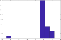
Figure 3. Eigenvalues of the Jacobian evaluated in one solution fulfilling C1-2). The Plefka value is $0.073206039645813\ll 1$.

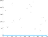
(a) Number of iterations (y-axis) fulfilling criteria C1-2) for negative $\varepsilon=-0.705-j\cdot 0.001,j=0,\ldots,20$ vs. disorder realisations (x-axis).

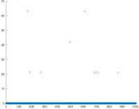
(b) Number of iterations (y-axis) fulfilling criteria C1-2) for positive $\varepsilon=0.705+j\cdot 0.001,j=0,\ldots,20$ vs. disorder realisations (x-axis).

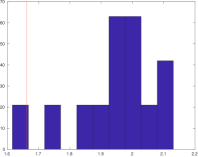
(c) Histogram of TAP FE satisfying C1-2) with positive $\varepsilon=0.705+j\cdot 0.001,j=0,\ldots,20$. The red line corresponds to the 2RSB Parisi FE.

Figure 4. $\varepsilon$-Banach: 500 start values close to the facets of the hypercube, 1000 disorder realizations. 1000 iterations for each start value and $\varepsilon$. Since the Parisi FE is an upper-bound [15], fixed points to the right of the red line in (C) must be rejected.

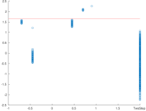
(a) TAP FE of all iterations landing inside the hypercube. The rightmost line of blue dots corresponds to 2SteB. Red is the Parisi FE (within the 2RSB approximation).

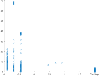
(b) Plefka-values (y-axis) of all iterations (x-axis): the large values ($\text{Plefka}\left(\bm{m}^{(k)}\right)\gg 10$) correspond to (unviable) iterates falling out of the hypercube. The red line is at $y=1$.

Figure 5. $\varepsilon$-Banach vs. 2SteB: 1000 uniformly chosen initializations, 1000 iterations each. One clearly evinces that 2SteB comes, in low temperature, to a stall: the algorithm doesn’t even come close to a reasonable TAP FE (Figure A). In case of $\varepsilon$-Banach, two choices lead to reasonable TAP free energies, but caution is needed: positive $\varepsilon=0.5$ yields solutions violating Plefka’s criterion (Figure B). Only negative $\varepsilon\approx-0.7$ lead to viable solutions: a numerical analysis of these is presented in Figure 6.

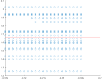
(a) TAP FE (y-axis) vs. $\varepsilon$ (x-axis).

(b) TAP FE (y-axis) of the realizations (x-axis).

(c) TAP FE Histogram.

Figure 6. $\varepsilon$-Banach: TAP FE of all solutions satisfying C1-2), 500 initializations close to the facets of the hypercube, 1000 disorder realizations, $\varepsilon=-0.705-0.001\cdot j$ for $j=0,\ldots,20$. Red is the 2RSB Parisi FE.

3.3. One, or more solutions?

The Parisi theory predicts, in low temperature, a large number of TAP solutions per realization. As can be evinced from Figure 7 below, numerical evidence for this is hard to come by: all solutions differ only after the 7th digit.

Figure 7. $\ell_{\infty}$-Distance (MAE) to a reference solution, C1-2) being satisfied, found by $\varepsilon$-Banach in 1000 realizations, each with 500 start values close to the facets of the hypercube, and $\varepsilon=-0.705-0.001\cdot j,j=0,\ldots,20$.

The crux of the matter seems to lie in the following: upon closer inspection, one finds that even after 1000 iterations, solutions (barely, but) still move. We have thus performed a more accurate numerical study, thereby recursively validating a fixed point as new whenever its $\ell_{\infty}$-distance to all previously validated is greater than $10^{-7}$. In order to facilitate the search for viable solutions we have also increased the accuracy of the $\varepsilon$-mesh: the outcome is summarized in Figure 8 below.

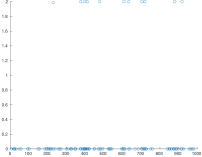
(a) As in Fig. 7, but finer $\varepsilon$-mesh.

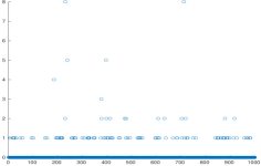
(b) # solutions per realization.

Figure 8. Iterations satisfying C1-2), and $\varepsilon=-0.505+0.001\cdot j,j\leq 250$.

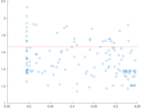
(a) For each $\varepsilon$ all TAP free energy values of all different solutions found.

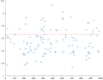
(b) TAP FE of all realizations and all different solutions.

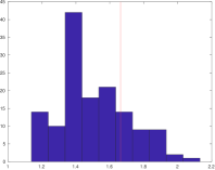
(c) Histogram of the TAP free energy values of all different solutions found.

Figure 9. TAP FE as in Fig. 6, but with $\varepsilon=-0.505+0.001\cdot j,j\leq 250$.

All fixed points appearing in Figure 9 satisfy C1-2): one evinces that $\varepsilon$-Banach has indeed found multiple solutions. However, many of these still yield TAP FE larger than the Parisi FE and must therefore be discarded. We believe this to be yet another instance of the aforementioned issue of unknown convergence criteria for the TAP-Plefka expansion.

References

- [1] Adhikari, Arka, Christian Brennecke, Per von Soosten, and Horng-Tzer Yau. Dynamical Approach to the TAP Equations for the Sherrington-Kirkpatrick Model. J. Stat. Phys. 183, 35 (2021).
- [2] de Almeida J.R.L, and David J. Thouless. Stability of the Sherrington-Kirkpatrick solution of a spin glass model. J. Phys. A: Math. Gen. 11, pp. 983-990 (1978).
- [3] Alt, Johannes, László Erdős, Torben Krüger and Dominik Schröder. Correlated random matrices: Band rigidity and edge universality. Ann. Probab. 48 (2) 963 - 1001 (2020).
- [4] Anderson, Greg, Alice Guionnet and Ofer Zeitouni. An introduction to random matrices. Cambridge University Press (2011).
- [5] Aspelmeier, T., Blythe, R. A., Bray, A. J., and Moore, M. A.. Free-energy landscapes, dynamics, and the edge of chaos in mean-field models of spin glasses. Physical Review B, 74(18), 184411. (2006)
- [6] Bolthausen, Erwin. An iterative construction of solutions of the TAP equations for the Sherrington–Kirkpatrick model. Commun. Math. Phys. 325, 333–366 (2014).
- [7] Bolthausen, Erwin. A Morita type proof of the replica-symmetric formula for SK. In: Statistical Mechanics of Classical and Disordered Systems. Springer (2019).
- [8] Celentano, Michael, Zhou Fan, and Song Mei. Local convexity of the TAP free energy and AMP convergence for Z2-synchronization. arXiv:2106.11428 (2021).
- [9] Chen, Wei-Kuo. On the Almeida-Thouless transition line in the SK model with centered Gaussian external field. arXiv:2103.04802 (2021).
- [10] Drazin, Michael P. and Emilie V. Haynsworth. Criteria for the reality of matrix eigenvalues. Math. Zeitschr. 78, 449-452 (1962).
- [11] Sherrington, David, and Scott Kirkpatrick. Solvable model of a spin-glass. Physical review letters 35.26: 1792 (1975).
- [12] Talagrand, Michel. Mean field models for spin glasses. Springer (2011).
- [13] Mézard, Marc, Giorgio Parisi, and Miguel A. Virasoro. Spin glass theory and beyond. World Scientific, Singapore (1987).
- [14] Chen, Wei-Kuo, Dmitry Panchenko, and Eliran Subag. The generalized TAP free energy. arXiv:1812.05066 (2018).
- [15] Guerra, Francesco. Broken replica symmetry bounds in the mean field spin glass model. Comm. in Math. Phys. Vol. 233 (2002).
- [16] Plefka, Timm. Convergence condition of the TAP equation for the infinite-ranged Ising spin glass model. Journal of Physics A: Mathematical and general 15.6 (1982): 1971.
- [17] Tao, Terence. Topics in random matrix theory. AMS (2012).
- [18] Thouless, David J., Philip W. Anderson, and Robert G. Palmer. Solution of ‘solvable model of a spin glass’. Philosophical Magazine 35.3 (1977): 593-601.