Automated SpectroPhotometric Image REDuction (ASPIRED)

Abstract

We provide a suite of public open-source spectral data-reduction software to rapidly obtain scientific products from all forms of long-slit-like spectroscopic observations. Automated SpectroPhotometric REDuction (ASPIRED) is a Python-based spectral data-reduction toolkit. It is designed to be a general toolkit with high flexibility for users to refine and optimize their data-reduction routines for the individual characteristics of their instruments. The default configuration is suitable for low-resolution long-slit spectrometers and provides a quick-look quality output. However, for repeatable science-ready reduced spectral data, some moderate one-time effort is necessary to modify the configuration. Fine-tuning and additional (pre)processing may be required to extend the reduction to systems with more complex setups. It is important to emphasize that although only a few parameters need updating, ensuring their correctness and suitability for generalization to the instrument can take time due to factors such as instrument stability. We compare some example spectra reduced with ASPIRED to published data processed with iraf-based and STARLINK-based pipelines, and find no loss in the quality of the final product. The Python-based, iraf-free ASPIRED can significantly ease the effort of an astronomer in constructing their own data-reduction workflow, enabling simpler solutions to data-reduction automation. This availability of near-real-time science-ready data will allow adaptive observing strategies, particularly important in, but not limited to, time-domain astronomy.

1 Introduction

With major global investments in multiwavelength and multimessenger surveys, time-domain astronomy is entering a golden age. In order to maximally exploit discoveries from these facilities, rapid spectroscopic follow-up observations of transient objects (e.g., supernovae, gravitational-wave optical counterparts, etc.) are needed to provide crucial astrophysical interpretations.

Part of the former OPTICON project coordinates the operation of a network of largely self-funded European robotic and conventional telescopes, collating common science goals and providing the tools to deliver science-ready photometric and spectroscopic data in near real time. The goal is to facilitate automated or interactive decision-making, allowing “on-the-fly” modification of observing strategies and rapid triggering of other facilities. As part of the network’s activity, a software development work package was commissioned under the working title of Automated SpectroPhotometric REDuction (ASPIRED), coordinated on Github.

The “industrial standard” of spectral and image reduction is undoubtedly the iraf framework (Tody, 1986, 1993). It has powered many reduction engines in the past and present. However, unfortunately, the National Optical Astronomy Observatory discontinued the support of the software in 2013, and it is now entirely relying on community support. The STARLINK library (Currie et al., 2014; Berry et al., 2022) includes substantial resources for data-reduction tasks in the Figaro package. It was first initiated in 1980 under the STARLINK Project, which became defunct in 2005, but the software survived, and its maintenance effort has since transferred to the East Asian Observatory. It also comes with a Python wrapper to enable low-level code access from high-level programs. These software tools have made significant contributions to the entire astrophysics community. They are very often overlooked when they are so deeply embedded into many systems, and users do not interact directly with them in this era of big data and high data rates. However, such tools are not always available. Many smaller facilities and individual users are still required to commission their own data-reduction routines. Existing powerful libraries and tools also come with a few drawbacks; the most notable obstacles concern the ease of installation and linkage of libraries, which users often find difficult.

In this generation of user-side astronomy data handling and processing, as well as the emphasis on computing courses for scientists, Python is among the most popular languages due to its ease to use with a shallow learning curve, readable syntax and simple way to “glue” different pieces of software together. Its flexibility to serve as a scripting and an object-oriented language makes it useful in many use cases: developing visual tools with little overhead, prototyping, web-serving, and compiling if desired. While this broad range of functionality and high-level usage make it relatively inefficient. Python is an excellent choice of language for building wrappers on top of highly efficient and well-established codes. Some of the most used packages, scipy (Virtanen et al., 2020) and numpy (Harris et al., 2020), are written in Fortran and C, respectively, to deliver high performance. Multithreading and multiprocessing are also possible with built-in and other third-party packages, such as mpi4py (Dalcin et al., 2011).

Various efforts are being made to develop software for the current and next generation of spectral data reduction. For example, PypeIt (Prochaska et al., 2020b, a) is designed for tailor-made reduction for a range of instruments, and PyReduce (Piskunov et al., 2021) is designed for optimal echelle spectral reduction (but only handles sky subtraction if a sky frame is provided). In the Astropy “universe” (Astropy Collaboration et al., 2013, 2018), specreduce (Pickering et al., 2022) is likely to be the next-generation, user-focused data-reduction package of choice, but it is still in early stages of deployment at the time of writing. pyDIS has all the essential ingredients for reducing spectra but has been out of maintenance since 2019, and specutils handles spectral analysis and manipulation but not the reduction itself.

In ASPIRED, we have a different vision of how and what should be abstracted from the users. Instead of providing a ready-to-go “black box” suited for a specific instrument or observations made under particular conditions, we provide a toolkit that is as general as possible for users to have a set of high-level data-reduction building blocks with which process the data in the ways most appropriate to their instruments and observations. This shifts more of the work and maintenance to the user end, but allows rapid modification of the data-reduction workflow to any changes in the instrumental configuration (such as a detector being refitted, or the detector plane shifted and rotated by a few pixels during engineering work) and to new instruments. ASPIRED is thus especially useful for works that repeatedly make use of multiple spectrographs requiring rapid follow-ups. Using ASPIRED only requires basic coding skills acquired by most graduate-level astronomers. Similar to iraf, PypeIt and other open-source software, we welcome and encourage users to provide feedback as well as to contribute to the code base.

We use the SPRAT spectrograph (Piascik et al., 2014) mounted on the Liverpool Telescope (LT) as our “first-light” instrument for development. ASPIRED is currently used by the transient science research group at Tel Aviv University for a proprietary spectral data-reduction pipeline of the Las Cumbres Observatory FLOYDS instrument. It is also known to be used for quick-look reduction of data obtained by the MISTRAL spectrograph mounted on the 1.93 m telescope at the Observatoire de Haute-Provence. However, as mentioned, we aim to allow high-level tools for users to build and fine-tune their pipelines to support a wide range of configurations (Lam et al., 2022; Lam, 2023). As of the time of writing, we have used ASPIRED to reduce data from the William Herschel Telescope Intermediate-dispersion Spectrograph and Imaging System (WHT/ISIS) and the Auxiliary-port CAMera (ACAM; Benn et al., 2008), the Las Cumbres Observatory FLOYDS (Las Cumbres/FLOYDS; Brown et al., 2013), the Gemini Observatory Gemini Multi-Object Spectrographs’s long-slit mode (Gemini/GMOS-LS; Hook et al., 2004), the Gran Telescopio Canarias Optical System for Imaging and low-Intermediate-Resolution Integrated Spectroscopy (GTC/OSIRIS; Cepa et al., 2000), the Telescopio Nazionale Galileo Device Optimised for the LOw RESolution (TNG/DOLORES; Molinari et al., 1999), the Very Large Telescope FOcal Reducer/low dispersion Spectrograph 2 (VLT/FORS2); and the Southern Astrophysical Research Telescope Goodman High Throughput Spectrograph (SOAR/GHTS Clemens et al., 2004). We show examples of these reductions in Section 5, and excerpts of example codes in Appendix A.

This article is organized as follows. Section §2 covers the development and organization of the software. Then, we discuss the details of the spectral image-reduction procedures in Sections §3 and 4. In Section §5 we show a few example spectra and compare then with published reductions. Section §6 explains how ASPIRED can be installed. Finally in Section §7, we summarize and discuss future plans.

This article is not intended to serve as an API document, nor as a review of the various methods concerning spectral extraction. Only the high-level descriptions and the scientific and mathematical technicalities that are important to the data-reduction processes are discussed here.

2 Development and Structure of ASPIRED

One of the development goals of ASPIRED is to design a piece of software that is as modular and portable as possible, such that it is operable on Linux, Mac and Windows systems (while software for astronomy and astrophysics are strongly leaning toward Unix systems, Windows has the highest market share worldwide; furthermore, demographically it is the common choice among university-managed computing systems, students and lower-income countries). On top of that, ASPIRED is designed to rely on as few external dependencies as possible. The ones we do use are those that would require a substantial programming effort to reproduce and have a proven track record of reliability and/or plan to remain maintained in the foreseeable future. The explicit top-level dependencies are – astros-crappy (van Dokkum, 2001; McCully et al., 2018) Astropy (Astropy Collaboration et al., 2013, 2018), ccdproc (Craig et al., 2017), numpy (Harris et al., 2020) plotly (Plotly Technologies Inc., 2015), rascal (Veitch–Michaelis & Lam, 2020a), scipy (Virtanen et al., 2020), spectresc (Carnall, 2017; Lam, 2023), specutils (Earl et al., 2023), and statsmodels (Seabold & Perktold, 2010).

We host our source code on Github, which provides version control and other utilities to facilitate its development. It uses git, issue and bug tracking, high-level project management, and automation with Github Actions upon each commit for the following:

1. Continuous integration to install the software on Linux, Mac and Windows systems, and then perform unit tests with pytest (Krekel et al., 2004) over most of the functions in multiple versions of Python.

2. Generating test coverage reports with coveralls which identifies the lines in the source code that are missed from the tests to assist us in maximizing the test coverage.

3. Continuous deployment through PyPI that allows immediate availability of the latest numbered version.

4. Version tracking of the depending packages with pull request is generated automatically (and the software is tested upon any update of the dependencies).

5. Generating API documentation powered by sphinx which scans for the decorators and automatically formats the written documentation (docstrings) into interactive html pages that can also be exported as a PDF file, and are hosted on Read the Docs${}^{\ref{rtd}}$.

The initial work package divided the project broadly into three high-level independent components, which we now detail.

Graphical User Interface
(Not in active development)

In the beginning, we commissioned a prototype of the graphical user interface with Electron, which wraps on top of ASPIRED without needing to adapt the code. Such a setup works seamlessly for a few reasons. First, Python is an interpreter; it can execute in run time. It is hence straightforward to run a Python server to interact with an Electron instance. Second, Plotly has a good balance in generating interactive and static plots; it requires little effort to interact with both Python and Electron. Third, there is a JavaScript version of SAOImageDS9, JS9, that allows rapid and easy interactive image manipulation with an interface that astronomers are accustomed to (Joye & Mandel, 2003; Mandel & Vikhlinin, 2022). Electron and JS9 work like a web service; this prototype also shows that an ASPIRED graphical user interface can be deployed as an online tool. Such a high level of interactivity is, however, no longer in active development and is only served as a one-off technology demonstration of its capability.

Arc Fitting for the Pixel-Wavelength Relation (a Concurrent Development)

The wavelength calibration process involves identifying distinctive emission lines from an arc-lamp spectrum, to which a function such as a polynomial can be fit to map the pixel position to the wavelength value. Manual calibration is straightforward but tedious: first, a user has to locate the peaks of an arc spectrum in pixel space. Then, they have to assign a wavelength to each peak based on the emission lines present from the element(s) of the arc lamp. Finally, the function to map pixel values to a set of wavelengths is found. Typically a list of known strong calibration lines is used, as provided by the instrument operators in the form of an atlas or a template calibration spectrum. Automation via template matching is a viable and commonly used approach for spectral calibration if the instrument configuration is stable (Prochaska et al., 2020a). However, this introduces a strong dependency on instrument-specific properties (such as the vacuum/contamination condition of the lamp, the combination of elements in the lamp, the vignetting on the focal plane, the response as a function of wavelength across the detector, and saturation issues). There is also noise in peak-finding routines, for example due to detector noise or quantization (e.g. not using subpixel peak finding), as well as complications due to blended lines. Providing a general, template-free tool for such a purpose for a range of specifications is far from easy, but would be much more flexible for cases when templates are unavailable or the instrument configuration changes often.

In ASPIRED, the wavelength calibration module is powered by the RANdom SAmple Consensus (RANSAC) Assisted Spectral CALibration  (rascal, Veitch–Michaelis & Lam 2020b, a, Veitch-Michaelis & Lam, in preperation) library, a concurrent software development project. rascal does not require templates and is designed to work with an arbitrary instrument configuration. Users are only required to supply a list of calibration lines (wavelengths), a list of peaks (pixels), and some knowledge (e.g. minimum and maximum wavelength limits) of the system to obtain the most appropriate pixel-to-wavelength solution. rascal builds on the work by Song et al. (2018), which searches only for plausible sets of arc line/peak correspondences that follow a linear approximation. RANSAC (Fischler & Bolles, 1981) is used to fit a higher-order polynomial model to the candidate correspondences robustly. rascal extends this strategy to consider the top $N$ sets of linear relations simultaneously: for each peak (pixel), the most common best-fit atlas line (wavelength) is chosen from those $N$ subsets that have a merit function better than a given threshold. This acts like a piecewise linear fit and allows us to extract most of the correct matches from both the red and blue ends of the spectrum - a feature that was not available in Song et al. (2018).

Data Reduction and Other Calibrations
(This Work)

This is the core of ASPIRED, which mainly handles the spectral extraction and calibration processes. At the user level, the software is organized into two main parts: image_reduction and spectral_reduction. They are designed to be as modular as possible. Users are free to use third-party reduction tools to perform part(s) of the reduction process and return to continue the reduction with image_reduction and spectral_reduction.

In addition, the data structure class SpectrumOneD handles the data and metadata of the extracted information. This provides a uniform format to store the metadata and the extracted data throughout the entire spectral extraction process. Since multiple spectra can be extracted from a TwoDSpec object (e.g., extended target or multiple targets aligned on the slit), each extracted spectrum is stored in an independent SpectrumOneD object that gets passed from a TwoDSpec object. In astronomy, the handling of observational data is almost exclusively done with FITS files, but they are not human-readable. In view of that, ASPIRED provides input and output handling of FITS files, and outputs in a CSV format. All the higher-level functions are wrappers on top of a spectrumOneD object.

3 Image Reduction

ASPIRED only intends to provide image-reduction methods for bias, dark, and flat corrections. It is sufficient for simple instrumental setups, which are the primary targets of ASPIRED, e.g., a long-slit spectrograph with a rectilinear two-dimensional spectrum illuminated on the detector plane, i.e., where the dispersion and spatial directions are perfectly perpendicular to each other across the entire detector plane. In systems with more complex optical designs, for example instruments with multiple nonparallel spectra illuminated on the detector plane, ASPIRED is not immediately usable. Extra image manipulation is needed to further transform the data into simpler forms that ASPIRED can handle. In the FLOYDS reduction example below, we demonstrate that it is possible to extract two nonparallel curved spectra from a single two-dimensional image. This is possible only because the two spectra (first-order red and second-order blue) that are simultaneously imaged by the detector can be cleanly separated before spectral reduction, and each spectrum is treated independently.

This module allows mean-, median-, and sum-combining, subtracting and dividing by dark, bias, and flat frames. The FITS header of the first light frame provided is retained in the reduced product, while the headers from the other frames are not stored – only the file paths are appended to the end of the FITS header. The FITS file is defaulted to contain an empty PrimaryHDU with the process data stored in the first ImageHDU extension as recommended in the FITS Standard document, but it can also be stored directly in the PrimaryHDU as most users opt for. Many forms of interactive and static images can be exported, powered by the Plotly image renderer.

This module only allows basic image reduction; users have to rely on third-party software to correct for any other effects before continuing the reduction with spectral_reduction.

4 Spectral Reduction

In the highest-level terms, ASPIRED’s spectral-reduction procedures after image reduction include (i) identifying and tracing the spectrum(a), (ii) correcting for image distortion, (iii) extracting the spectrum(a), (iv) performing wavelength calibration of the science target and a standard star, (v) computing the sensitivity function using the standard star, (vi) performing atmospheric extinction correction; and, finally (vii) removing the telluric absorption features, (viii) resampling, and (ix) exporting the data. We omit a few other processes, which we believe should be considered as part of the postextraction processes or spectral analysis and manipulation. There are many sophisticated software packages with good and long track records to handle these processes post hoc. For example, sky-glow subtraction with Skycorr (Noll et al., 2014), or telluric absorption removal without supplementary calibration data with MoleFit (Smette et al., 2015; Kausch et al., 2015).

The spectral_reduction is a large module that covers both the two-dimensional and one-dimensional operations through the TwoDSpec and OneDSpec classes, respectively. The former provides image rectification, spectral tracing, spectral extraction of the target and the arc, and locating the peaks of the arc lines. The latter performs wavelength calibration (with the WavelengthCalibration class), flux calibration (with the FluxCalibration class), atmospheric extinction correction, telluric absorption correction, and spectral resampling. Diagnostic images can be exported at each step of the two- and one-dimensional operations. This also includes the wavelength calibration diagnostic that wraps around rascal and uses its native plotting capability. Since the flux calibration has to be performed with a standard star spectrum, it is necessary for the OneDSpec object to have information on both the target and the standard one-dimensional spectra. Thus, a OneDSpec object keeps a dictionary of lists: – science_spectrum_list and standard_spectrum_list. At the time of writing, ASPIRED only supports wavelength calibration from one (total stacked) arc frame and flux calibration from one (total stacked) standard star frame.

The following describes the technical details of the nine reduction steps mentioned above. We use the following convention throughout this article: the spectral image is dispersed on the detector plane such that the left side (small pixel number) corresponds to the blue part of the spectrum and the right side (large pixel number) to the red part in the dispersion direction, while the direction perpendicular to it is the spatial direction.

spectral_reduction accepts images that are rotated or flipped compared to the description above, but extra arguments have to be provided in the initialization step to set the data into the orientation as defined above.

4.1 Spectral Identification and Tracing

Conventionally, to obtain the position of a spectrum in a frame (i.e., a trace), the center of the spectrum in the dispersion direction is first identified. Then, a choice of algorithm scans across the spectral image to identify the spectral position over the entire dispersion direction. In ASPIRED, the ap_trace function works by dividing the two-dimensional spectrum into subspectra. Then, each part is summed along the dispersion direction before cross-correlating with the adjacent subspectra, using an optional variable scaling factor that models a linear change in the width of the trace (this optional scaling factor is turned off by default). This allows both the shift and the scaling of the spectrum(a) along the dispersion direction to be found simultaneously. The middle of the two-dimensional spectrum is used as the zero-point of the procedure. This tracing procedure is illustrated in Figure 1, and described in more detail as follows:

1. The input two-dimensional spectrum is divided into nwindow overlapping subspectra.

2. Each subspectrum is summed along the dispersion direction in order to improve the signal(s) of the spectrum(a) along the spatial direction to generate the line-spread function of that subspectrum.

3. Each line-spread function is upscaled by a factor of resample_factor to allow for subpixel correlation precision. This utilizes the scipy.signal.resample function to fit the spatial profile with a cubic spline.

4. The $i$th line-spread function is then cross-correlated to the $(i+1)$th line spread function. The shift and scale correspond to the maximum correlation within the tolerance limit, tol, and are stored.

5. The shifts relative to the central subspectrum are used to fit for a polynomial solution with a constant arbitrary offset.

6. While the spatial spectra are cross-correlated, they are also aligned and stacked to find the peak of the line-spread profile. Peak finding is performed with scipy.signal.find_peaks and returns the list of peaks sorted by their prominence, which is defined as the maximum count of the peak subtracted by the local background. The total stacked line-spread profile is fitted with a Gaussian function to get the spread of the spectrum (standard deviation). This would not be used in the case of top-hat extraction (see section §4.3).

Manually supplying a trace (determined a priori or copied from another observation) is possible with the add_trace function. This is particularly useful for faint and/or confused sources that are beyond the capability of automated tracing. For example, if there is a faint transient source on top of a galaxy, a manual offset may be needed for extraction if the host is dominating the flux to a level that forced extraction is necessary. For an optical design where the source spectrum is always illuminated at the same pixels of a detector, it is possible to reuse the trace from the standard frame for spectral extraction of the science target.

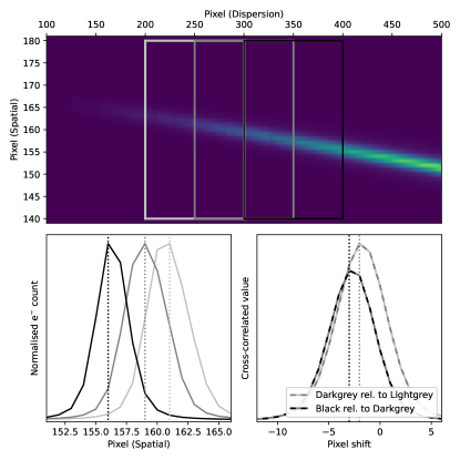
Figure 1: Top: a significantly tilted spectrum is used to illustrate how cross-correlation is used to find the shift between neighboring subspectra with a resampling factor of 1.0. The light gray, dark gray and black boxes are three example subspectra. Bottom left: the three subspectra are summed in the dispersion direction to generate the three profiles that are cross-correlated to compute the shift. Bottom right: the cross-correlated function for the light gray subspectrum relative to the dark gray subspectrum (plotted in alternating light and dark gray dashes), and the one for the black subspectrum relative to the dark gray subspectrum (plotted in alternating dark gray and black dashes).

In the cross-correlation process, ASPIRED supports the upsampling of the data. Because more than one target could be incident on the slit, we do not attempt to fit any profile at this stage. Hence, the shifts found are always quantized to an integer pixel level. However, the polynomial fitted through the shifts as a function of the dispersion direction is a continuous function. The final precision depends on the upsampling rate. If no upsampling is performed and the spectrum is tilted by one pixel across the entire range of dispersion, for example, this step will not be able to get the tilt correctly. By default, we set the upsampling rate to four. This should be sufficient to correct for a tilt in the spectrum as little as 0.25 pixels across the entire range of dispersion.

4.2 Image Rectification

In some cases, a spectrum on the detector plane is not only tilted, but it is also sufficiently distorted that the spatial and dispersion direction (in the detector’s Cartesian coordinates) are no longer orthogonal to each other. While this does not cause any complication in the tracing process, the extraction has to be performed along a curve so that the process is no longer a one-dimensional process. Without proper weighting in extracting flux at the subpixel level, significant under- or oversubtraction of the sky background can occur. More complex methods have to be used to extract the spectra directly (e.g. Piskunov et al., 2021), as implemented in PyReduce, which can optimally extract highly distorted spectra. However, PyReduce cannot perform sky subtraction using the “wings” in the sky region on either side of the line-spread profile. This has limited the usage of PyReduce in typical single-frame extractions without accompanying sky observations exposed using an identical slit setting. In ASPIRED, a TwoDSpec object uses the spectral trace for alignment in the spatial direction, and uses the sky emission lines, and optionally coadded with the arc image, for alignment in the dispersion direction. This process is to perfectly align the two-dimensional spectral coordinate system with the detector’s $x-y$ axes. Coadding the arc frame for the procedure can improve the reliability of the rectification, as more bright lines are available in the coadded image for computing the rectification function that shifts and scales the image.

The rectification is done independently first in the spatial direction and then in the dispersion direction. In the spatial direction, the process only depends on the trace. Each column of pixels is (scaled and) shifted by resampling it to align to the center of the spectrum (middle panel of Fig. 2). This process usually produces a spectrum that is tilted or curved in only the dispersion direction. Therefore, a similar procedure has to be performed in the dispersion direction. However, lines are not traced in this direction. In order to find the size of the scaling and shifting, we repeat the tracing procedures in Sec. 4.1 from steps 1 through 5 in the perpendicular (dispersion) direction. A first- or second-order polynomial is usually sufficient to fit the shift as a function of the number of pixels from the trace. Then, the spectral image is resampled a second time but only in the dispersion direction. The final result is shown in the bottom panel of Fig. 2.

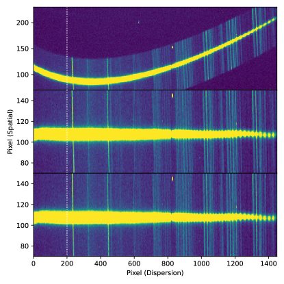
Figure 2: A two-dimensional spectrum from Las Cumbres/FLOYDS is used to demonstrate the rectification procedure. The dotted white line is aligned in the spatial direction to serve as a visual guide. Top: the trimmed image of a FLOYDS spectrum. Middle: the two-dimensional spectrum is resampled in the spatial direction based on the polynomial function of the trace. Bottom: the two-dimensional spectrum is resampled in the dispersion direction. The shifts and scales are found by cross-correlating the subspectra divided in the spatial direction. This is perpendicular to the tracing process.

At the time of writing, this process only works on a single trace. If more than one trace is found/provided, only the one with the highest prominence will be processed, where the prominence is defined as the maximum count of the peak subtracted by the local background. The resampling is performed with spectresc. It is possible to supply a set of precomputed polynomials to perform the rectification, which can significantly speed up the data-reduction process of a stable optical system.

4.3 Spectral Extraction

There are a few commonly used extraction methods; some work for all kinds of spectral images, and some only work with specific observing strategies (e.g. the flat-relative optimal extraction; Zechmeister et al. 2014). The standard textbook method is commonly called the top-hat extraction or the normal extraction. It simply sums the electron counts over a given size of the aperture and is robust and easy to use. However, this method does not deliver the maximal signal-to-noise ratio (S/N) from the available data. Various optimal extraction algorithms can maximize the S/N. They work by down-weighting the wings of the spectral profile, where almost all the photons come from the sky background rather than the source (see Fig. 3). The improvement is particularly significant for background-limited sources, which are the case in most observations (see Fig. 4). The extracted spectra and their associated uncertainties and sky-background counts can be plotted for inspection. The residual image can also be exported for diagnostics.

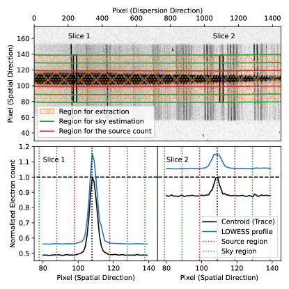
Figure 3: The same spectrum as in Figure 2. Top: the regions used for source and sky extractions are marked by the red and green boundaries. The light shade of orange hash marks the region that is used for spectral extraction. The two boxes show the two columns of pixels fitted with profiles in the bottom half of the figure (the boxes are inflated for clarity). Bottom: the independently normalized electron counts across the two slices; the much higher baseline on the right indicates a lower signal-to-background ratio. The vertical black dashed line is the centroid (trace) of the spectrum, the two red dashed lines mark the regions of the source, and the pairs of green dashed lines on each side of the centroid show the regions used for sky extractions, respectively. The black line is the measured spectral profile (data), and the blue line is the fitted LOWESS line-spread function (model), offset for clarity. The right panel illustrates how an extraction over a nonrectified two-dimensional spectrum can lead to an increased sky-background level.

Tophat/Normal Extraction

The top-hat extraction does not weight the pixels for extraction, so every pixel has an equal contribution to the source count. Thus, it is very robust in obtaining the total electron count across a slice of pixels. The sky-background count can be extracted from the regions outside the extraction aperture to be subtracted from the spectrum.

Horne-86 Optimal Extraction

Horne (1986, hereafter H86) is the golden standard of optimal extraction of spectra from modern electronic detectors. We follow the H86 process except for the profile modelling, where we provide three options: the first is a fixed Gaussian profile, the second uses LOcally Weighted Scatterplot Smoothing (LOWESS; Cleveland, 1979) regression to fit for a polynomial, and the third accepts a manually supplied profile.

The default option is to use the Gaussian fit because it is more robust against noise, cosmic-ray contamination, and artifacts. It is particularly useful in extracting a faint spectrum when the image is dominated by background noise as the Gaussian profile is constructed by fitting the line-spread function from the total stack of all the subspectra (as described in Sec. 4.1). LOWESS, on the other hand, would do a better job in fitting the profile of a resolved galaxy. In any case, the quality of the extraction from a valid profile should be at least as good as that performed with the top-hat extraction method.

Marsh-89 Optimal Extraction

Marsh (1989, hereafter M89) extends on the H86 algorithm by fitting the change in the shape and centroid of the profile from one end of the spectrum to the other. It is very suited for extracting a highly tilted spectrum where the tilting direction is aligned with one direction in the $x$-axis or the $y$-axis of the detector. The algorithm still relies on the assumption that the spatial and dispersion directions are orthogonal across the entire frame (in the detector pixel coordinates). In ASPIRED, we adapt Prof. Ian Crossfield’s set of public python 2 code for astronomy to python 3.

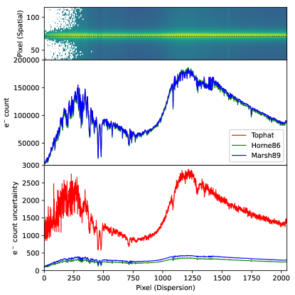
Figure 4: Top: the VLT/FORS2 spectrum and the trace of the standard star LTT 7379. Middle: the extracted spectra in electron counts using the three extraction methods are very similar. Bottom: the uncertainties with the three extraction methods in units of electron counts. The top-hat method is clearly noisier than the two optimal methods. Extractions using the Horne86 and Marsh89 algorithms produce almost identical outputs.

4.4 Wavelength Calibration

As mentioned, the wavelength calibration is powered by rascal, which is a concurrent development to this work. All the public functions from rascal are available in ASPIRED so that users can have fine control over the calibration. It works by applying a Hough transform to a set of peak-line (pixel-wavelength) pairs (i.e., Hough pairs), and then identifying the most probable set of Hough pairs that can be described by a polynomial function which satisfies the required residual tolerance limit (see more details in Veitch–Michaelis & Lam 2020a)

The diagnostic plots available are the set provided by rascal. They include (i) the spectrum of the arc lamp extracted using the traces from the science and standard frames, wherein the peak of the arc lines are also marked; (ii) the Hough pairs and their constraints in the parameter space; and (iii) a plot showing the best-fit solution, the residual of the solution, and the pixel-wavelength relation (Fig. 5).

Alternatively, the polynomial coefficients for the wavelength calibration can be supplied manually, which would be useful for stable instruments in which the variations in the dispersion are negligible. All the lines in the range of 100 – 30000 Å available from the search form of the National Institute of Standards and Technology Physical Measurement Laboratory are included, but we strongly recommend providing arc lines manually since arc lamps, even of similar type, vary between manufacturers and the conditions.

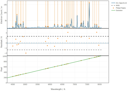
Figure 5: The native wavelength calibration diagnostic plots from rascal. Top: the arc is plotted in blue, the fitted peaks are marked by the orange dots. Middle: the residual plot shows the difference between the fitted peaks and the true wavelengths. Bottom: The pixel-wavelength function (green) is overplotted with the fitted peaks (orange).

4.5 Flux Calibration

ASPIRED is designed to address the common case where targets and reference standards are observed contemporaneously in close succession. It is well suited to constructing unsupervized, automated pipelines for stable and repeatable instruments. In such cases, an instrument sensitivity function can be created from several standard targets, stored and applied to many science target observations. At the time of writing, ASPIRED cannot construct a sensitivity function from multiple frames, but it can accept a user-supplied polynomial function to apply the calibration.

The process of deriving a sensitivity function is by comparing a wavelength-calibrated standard spectrum with the literature values to map the electron count to flux as a function of wavelength. All the standard stars available in iraf, on the Issac Newton Group of Telescopes web page, and on the European Southern Observatory (ESO) web page (Optical and UV Spectrophotometric Standard Stars) are available on ASPIRED. We call the set of data a library, and provide below the complete listing of sources and references for each of the libraries where available.

European Southern Observatory

The ESO standard spectra are grouped into five sets, they can be downloaded from the ESO site..

1. esoctiostan – CTIO standards from Hamuy et al. (1992, 1994)

2. esohststan – HST standards from Bohlin et al. (1995); Bohlin (1996)

3. esookestan – Oke standards from Oke (1990)

4. esowdstan – White dwarf standards from Bohlin et al. (1995)

5. esoxshooter – ESO VLT X-shooter standards from Moehler et al. (2014a, b)

Issac Newton Group of Telescopes

The Issac Newton Group of Telescopes (ING) listing is grouped into five sets by the last name of the authors.

1. ing_oke – Oke (1990) standards

2. ing_sto – Stone (1977) standards

3. ing_og – Oke & Gunn (1983) standards

4. ing_mas – Massey et al. (1988) standards

5. ing_fg – Filippenko & Greenstein (1984) standards

iraf Standards

The complete listing of iraf standards can be found online . References are included where they are available.

1. irafblackbody

2. irafbstdscal – KPNO IRS standards (i.e. those from the Henry Draper catalogue)

3. irafctiocal – The original CTIO standards Stone & Baldwin (1983); Baldwin & Stone (1984)

4. irafctionewcal – The updated CTIO standards Hamuy et al. (1992, 1994)

5. irafiidscal – KPNO IIDS standards Massey et al. (1988)

6. irafirscal – KPNO IRS standards Massey et al. (1988)

7. irafoke1990 – HST standards Oke (1990)

8. irafredcal – KPNO IRS standards & IIDS Massey et al. (1988) with wavelength beyond 8 370 $\mathrm{\AA}$

9. irafspechayescal – KPNO standards Massey et al. (1988)

10. irafspec16cal – CTIO standards Hamuy et al. (1992, 1994) at 16$\mathrm{\AA}$ interval

11. irafspec50cal – KPNO standards Massey et al. (1988); Massey & Gronwall (1990) at 50$\mathrm{\AA}$ interval

The calibration can be done in either AB magnitude or flux density (per unit wavelength). The two should give similar results, but the response functions found would not be equivalent because fitting to magnitudes is in logarithmic space and smoothing (see below) will have a different effect compared to flux fitting.

Smoothing

A Savitzky-Golay smoothing filter (Savitzky & Golay, 1964, hereafter, SG-filter) can be applied to the data before computing the sensitivity curve. This function works by fitting low-order polynomials to localized subsets of the data to suppress noise in the data at each point interval. It is similar to the commonly used median boxcar filter but uses more weighted information to retain information better while removing noise. This can be used independently or with continuum fitting (see below). By default, the smoothing is turned off, and when it is used it is defaulted to remove only significant noise (e.g. from unsubtracted cosmic-rays).

Continuum Fitting

It is optional for the sensitivity function to be derived from the continuum of the standard spectrum. This removes absorption lines in the standard spectrum. This process is strongly dependent on both the resolution of the literature and the observed standards, as well as the absorption lines present in them. The continuum is found using the specutils’s fits_continuum. This can remove any outlying random noise and absorption lines when computing the sensitivity. Users are reminded to be cautious with this procedure as removing the absorption features in computing the sensitivity function can significantly affect the flux calibration near the absorption features.

Sensitivity Function

The sensitivity function is computed by dividing the observed standard spectrum by the literature one and then interpolating the result using a spline or a polynomial function (Fig. 6). This can be done with or without any presmoothing and/or continuum fitting. In case of a high-resolution literature standard spectrum (e.g. the ESO X-Shooter standards), the absorption-line profiles should be used as part of the sensitivity computation, while in the case of the standard stars from Oke (1990), which removed absorption lines when producing the standard spectra, a smooth continuum of the observed spectrum should be used for computing the sensitivity function. Users can also manually supply a sensitivity function as a callable function that accepts a wavelength value and returns the $\log$ of the sensitivity value at that wavelength. When such a function is provided manually, it is assumed to be in the units of flux per second.

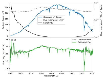
Figure 6: Top: the extracted standard spectrum in electron counts (blue), the literature spectrum in units of flux density (orange), and the sensitivity function (y-axis on the right; black). Bottom: the literature spectrum (same as the one above) is plotted in orange, and the calibrated observed spectrum is plotted in green.

4.6 Atmospheric Extinction Correction

ASPIRED currently has four built-in atmospheric extinction curves (Fig. 7):

1. Roque de los Muchachos Observatory, Spain (La Palma, 2420 m).

2. Mauna Kea Observatories, USA (Big Island, Hawaii, 4205 m; Buton et al., 2013).

3. Cerro Paranal Observatory, Chile (Atacama Desert, 2635 m; Patat et al., 2011).

4. La Silla Observatory, Chile (Atacama Desert, 2400 m).

These curves describe the extinction in magnitude per air mass as a function of wavelength, roughly between $3000$ and $10000$ Å. Alternatively, a callable function in the appropriate units can be supplied to perform the extinction correction. The air mass of the observation can be found from the header if it is reported using the conventional keywords for air mass.

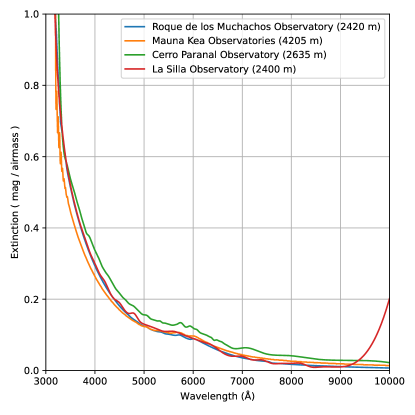
Figure 7: Extinction curves measured at Roque de los Muchachos Observatory (2420 m; blue), Mauna Kea Observatories (4205 m; orange), Cerro Paranal Observatory (2635 m; green), and La Silla Observatory (2400 m; red). The extinction table of La Silla Observatory terminates at $9000$ Å. The rise at the red end of the curve is an undesired artefact due to extrapolation using a cubic spline. We are explicitly plotting this range to serve as a warning since we opt to preserve the raw data as provided without appending fake data points.

4.7 Telluric Absorption Removal

During the process of generating the sensitivity function, masks are used over the telluric regions to generate the telluric absorption profile from the standard star. The default masking regions are $6850-6960$ and $7580-7700$ Å only. This telluric profile can then be multiplied by a factor to be determined in order to remove the telluric absorption features in the science target. The best multiplicative factor is found by minimizing the difference between the continuum and the telluric-absorption-corrected spectrum simultaneously for both the sampled telluric regions (there are only two ranges in the default setting, but if more regions are provided, this process will apply to all of them simultaneously). An extra multiplier can be manually provided to adjust the strength of the subtraction. This is designed for manually fine-tuning the absorption factor; otherwise, it defaults to $1.0$.

4.8 Resampling

All the operations above are performed as a function of the native detector pixels. This includes the telluric absorption corrections as the telluric profile is generated in the standard spectrum pixel/wavelength coordinates. The correction applied to the target spectrum is performed using an interpolated function of the profile at the wavelengths of the target spectrum.

Many legacy software packages can only read the spectrum using the header information to create the wavelength coordinates using only three parameters: the wavelength of the first element of the spectral array, the bin width of each wavelength coordinate, and the length of the spectral array. This requires a uniformly sampled wavelength axis, which never happens naturally as there is always some level of image distortion at the detector plane. A resampling is necessary to turn the data into such a format.

The resampling is performed with the spectresc package. Although this package allows nonuniform wavelength spacing resampling, we are only using it for uniform resampling for the purpose of exporting the data as FITS files.

4.9 Output

At the time of writing, 22 types of output to CSV and FITS files are supported. Each CSV has the various exported data (see below) stored in a separate columns, while the FITS has the data stored in separate header data units (HDUs). Each spectrum is exported as a separate file. At the time of writing, the header is not exported when the output option is CSV. The options for output are as follows:

1. trace: two columns/HDUs containing the pixel coordinates of the trace and its width in the spatial direction.

2. count: three columns/HDUs containing the electron count of the spectrum, its uncertainty, and the sky background.

3. weight_map: one column/HDU for the extraction profile; in top-hat and horne86 extraction this is a one-dimensional array, while the marsh90 extraction returns a two-dimensional array.

4. arc_spec: three columns/HDUs for the one-dimensional arc spectrum, pixel coordinates of the arc line position (subpixel precision), and the pixel coordinates of the arc line effective position (e.g. accounting for chip gaps) in the dispersion direction.

5. wavecal: one column/HDU for the polynomial coefficients for wavelength calibration. The header contains the information regarding the polynomial type.

6. wavelength: one column/HDU for the wavelength at the native pixel position.

7. sensitivity: one column/HDU containing the sensitivity function of the detector as a function of the native detector pixel.

8. flux: three columns/HDUs containing the flux of the spectrum, its uncertainty, and the sky background.

9. atm_ext: one column/HDU containing the atmospheric extinction correction factor at each wavelength position.

10. flux_atm_ext_corrected: three columns/HDUs containing the atmospheric-extinction-corrected flux of the spectrum, its uncertainty, and the sky background.

11. telluric_profile: one column/HDU containing the telluric absorption profile from the standard spectrum.

12. flux_telluric_corrected: three columns/HDUs containing the telluric-absorption-corrected flux, uncertainty, and the sky background.

13. flux_atm_ext_telluric_corrected: three columns/HDUs containing the atmospheric-extinction-corrected and telluric-absorption-corrected flux, uncertainty, and the sky background.

14. wavelength_resampled: one column/HDU containing the wavelength at each resampled position.

15. count_resampled: three columns/HDUs containing the electron count of the spectrum, its uncertainty, and the sky background being subtracted during the extraction process at the resampled wavelength.

16. sensitivity_resampled: one column/HDU containing the sensitivity function of the detector as a function of resampled wavelength.

17. flux_resampled: three columns/HDUs containing the flux of the spectrum, its uncertainty, and the sky background at the resampled wavelength.

18. atm_ext_resampled: one column/HDU containing the atmospheric extinction correction factor at the resampled wavelength.

19. flux_resampled_atm_ext_corrected: three columns/HDUs containing the atmospheric-extinction-corrected flux of the spectrum, its uncertainty, and the sky background at the resampled wavelength.

20. telluric_profile_resampled: one column/HDU containing the telluric absorption profile from the standard spectrum at the resampled wavelength.

21. flux_resampled_telluric_corrected: three columns/HDUs containing the telluric-absorption-corrected flux, uncertainty, and the sky background at the resampled wavelength.

22. flux_resampled_atm_ext_telluric_corrected: three columns/HDUs containing the atmospheric-extinction-corrected and telluric-absorption-corrected flux, uncertainty, and the sky background at the resampled wavelength.

5 Validation

Being a flexible toolkit, ASPIRED is not designed to reduce data for a specific instrument. Instead, it can be customized to suit many configurations, as long as they are long-slit-like. We demonstrate this here with data products from eight different instruments, most of which have conventional long-slit settings. A summary of the following example reductions is tabulated in Table 1.

The purpose of the comparison made here is to demonstrate that the reductions are sufficiently consistent with representative spectra in the literature for a range of instruments and astrophysical sources. However, a full systematic comparison is beyond the scope of this work. Such a level of detailed validation might be required for any service providers who wish to adopt ASPIRED as their official reduction tool, and will be included in future work.

5.1 Example Data Reduction Results

In the case of Gemini/GMOS, a single spectrum is exposed onto three detectors, and each detector is read out with four amplifiers. The bias subtraction is also unconventional, so all the image data-reduction procedures have to be done outside of ASPIRED beforehand. We compare our reduction against the official one for the kilonova AT 2017gfo (McCully et al., 2017).

Las Cumbres Observatory/FLOYDS has a beam splitter to expose the first-order red beam and the second-order blue beam into two nonparallel curved spectra on a single chip. Both the northern and southern FLOYDS suffer from strong fringing effects. This is not handled natively through the API of ASPIRED. Instead, the correction was done by directly modifying the electron count of the OneDSpec object. The fringe subtraction workflow follows that of the official pipeline. Here, the Type II supernova iPTF14hls is used as an example for comparison (Arcavi et al., 2017).

LT/SPRAT is a high-throughput low-resolution spectrograph with a conventional optical design; in this case, we compare our reduction to that published for a nova shell, DO Aql, from a stack of four individual exposures (Harvey et al., 2020).

The VLT/FORS2 data of the helium accretor (AM CVn) V418 Ser, stacked from 21 individual exposures, is used as our last comparison (Green et al., 2020).

The first three spectra were compared against data reduction from iraf-based pipelines, while the last one is reduced with Molly (Marsh, 2019), which is built on top of STARLINK. All of our reductions are resampled to match the resolution in the equivalent published spectra. Our comparisons are shown in Figure 8.

Aside from the comparison against the independently and externally calibrated spectra above, we also illustrate a few cases of extractions concerning other use cases that ASPIRED is capable of dealing with. In the top set of spectra in Figure 9, the GTC/OSIRIS data show a blue large-amplitude pulsator with many resolved absorption lines in both the science and the standard targets (Feige 110;  McWhirter & Lam, 2022). With a poorly computed sensitivity curve, we expect many small bump features in the spectra and that their continuum would not agree in the overlapping wavelength range, as polynomials tend to run away at the edges of the fitted range of the wavelength solution. In the middle, the TNG/DOLORES case shows a simultaneous tracing of a common proper motion system (three bodies resolved as two components) containing an M dwarf and an eclipsing M dwarf–white dwarf binary (Keller et al., 2022), separated by 5” incident on the same long-slit in a single exposure. At the bottom is a set of three spectra taken with WHT/ISIS and ACAM. It demonstrates the reduction of a set of data with extremely low S/N for an ultracool white dwarf with a smooth blackbody-like spectrum (Lam et al., 2020). The tracing and extraction are only possible after careful cosmic-ray removal and trimming of the images. The spectral shapes of the ISIS spectra in both the blue and the red arms are in good agreement with the ACAM spectrum, and these independently flux-calibrated spectra agree well with each other in the overlapping wavelength ranges.

To summarize, our test cases cover the most commonly encountered possible problematic data – red- or blue-dominated spectra, narrow/broad absorption/emission lines, featureless spectra, closely spaced (resolved) line spectra and curved spectra – and demonstrate that ASPIRED can produce spectral products at a quality comparable to some selected published spectra.

Telescope/Instrument	Object Type	Grating	Arc
Conventional Long-slit Setup
GTC/OSIRIS	BLAP (ZGP-BLAP-09)	R2500U and R1000B	HgArNe
LT/SPRAT	Nova shell remnant (DO Aql)	600 l/mm	Xe
TNG/DOLORES	Common proper-motion and eclipsing system	LR-B	ArKrNeHg
	(ZTF J192014.13+272218.1)
VLT/FORS	AM CVn (V418 Ser)	600B	HeHgCd
WHT/ACAM	Ultracool white dwarf (PSO J180153.69+625420.24)	V400	CuAr
WHT/ISIS	Ultracool white dwarf (PSO J180153.69+625420.24)	R300B and R300R	CuAr
Other Setup
Las Cumbres/FLOYDS	Type II-P (iPTF14hls)	235 l/mm	HgArZn
Gemini/GMOS	Kilonova (AT 2017gfo)	R400 and B600	CuAr

Table 1: List of the eight targets used in Figures 8 & 9 in alphabetical order of the telescope names. See body text for references.

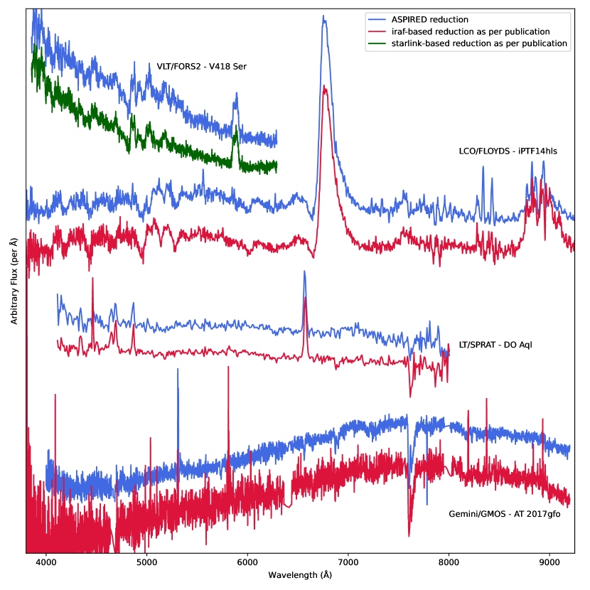
Figure 8: From top to bottom are the comparison spectra taken with VLT/FORS2, Las Cumbres/FLOYDS, LT/SPRAT and Gemini/GMOS in long-slit mode. The published FORS2 spectrum was reduced using Molly (green) powered by the STARLINK library. The other three (red) were reduced using the respective iraf-based pipelines. All spectra reduced with ASPIRED (blue) are optimally extracted using the Horne (1986) algorithm and resampled to match the respective published spectra. Telluric correction is applied using the default setting.

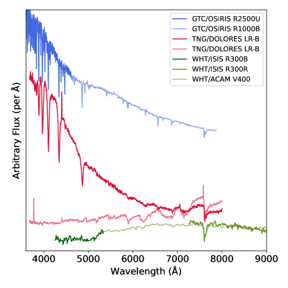
Figure 9: Example extractions of some special cases. Each set of spectra uses the same normalization. All spectra are optimally extracted using the Horne (1986) algorithm. The GTC/OSIRIS (top set in blue hue) spectra were flux calibrated in the shorter wavelengths where there are a lot of absorption features. With a bad sensitivity curve, we expect many small bump features in the spectra and that their continuum would not agree in the overlapping wavelength range, as polynomials tend to run away at the edges. The TNG/DOLORES (middle set in red hue) spectra were of two targets where the tracing was done simultaneously and then the extraction done sequentially. The WHT/ISIS and ACAM (bottom set in green hue) data demonstrate extracting a target with a very low S/N ratio. The independently flux-calibrated spectra agree well with each other in the overlapping wavelength ranges.

5.2 Repeatability

In order to demonstrate reproducibility and repeatability, we opt to calibrate the standard star BD33+2642 against Hiltner 102 on eight nights for which LT/SPRAT observed both on the same night during semester 2022 B. We require the transparency to be photometric, and the seeing be better than 2” as reported by the autoguider. Because of the robotic observing nature of the LT, standard stars are only taken at the beginning and at the end of the night. The data used were not taken immediately before or after each other, and therefore weather effects cannot be calibrated out. We only apply atmospheric extinction corrections and telluric absorption corrections. The spectra are consistent with each other to within 1%-2% (apart from the telluric absorption regions and at the H$\gamma$ line at 4340 Å that are observed at low detector efficiency; see Fig. 10).

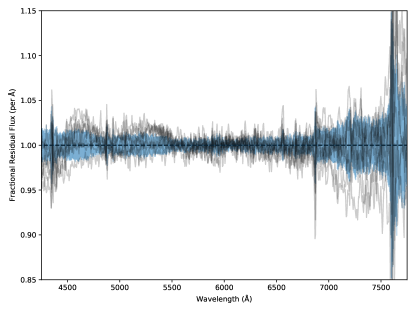
Figure 10: Fractional residual in the calibrated flux of BD 33+2642 using Hiltner 102 as a standard star taken with LT/SPRAT. Each gray line depicts the calibration residual between the median spectrum of the eight spectra taken on different nights. The blue area shows the one standard deviation of the scatter in the residual. The spikes above 5% residual are at the H$\gamma$ line at 4340 Å and the oxygen telluric features at 6869 and 7605 Å . The residuals that are larger on the two ends are expected as the S/N ratios drop with the detector efficiency on either side.

6 Distribution

ASPIRED is released under the BSD (3-Clause) License. The source code is hosted on Github. The DOI of each version can be found on zenodo: https://zenodo.org/record/4127294. For more straightforward installation, ASPIRED is also available with the Python Package Index (PyPI) so users can install the software with a single command:

>> pip install aspired

The latest stable version can be installed with

>> pip install git+https://github.com/
    cylammarco/ASPIRED@main

and the development version can be installed with

>> pip install git+https://github.com/
    cylammarco/ASPIRED@dev-v[Major].[Minor].X

Here, [Major]+ and [Minor]+ are the major and minor version numbers. \verbX+ is an actual character of the branch name, as we only use separate maintenance branches at the level of minor version granularity.

It is also possible to clone the entire repository and install with the setup script using

>> git clone [url to main/dev/a specific commit]
>> python setup.py

.

All the reduction scripts for the spectra used in this article can be found online . There are also example reduction scripts available from the companion repository ASPIRED-example which are tagged by version number starting from v0.4. This work is most accurately reflects the software release of the v0.5-series. We encourage users to reduce example spectra available in these repositories, using their own pipelines, for comparison.

7 Summary and Future work

We expect to continue the development and maintenance of ASPIRED in the future. Some of the main planned developments include the following:

1. Improving the quality of the flux calibration by carefully masking out the absorption lines in the standard spectra, and treating the high- and low-resolution templates differently.

2. Accepting arcs taken at different times and using the effective wavelength calibration solution over a long observing block.

3. Accepting standards taken at different times and computing the effective sensitivity function that takes into account the nonnegligible change in the flux of the target over a long observing block.

4. Exporting reduced spectra as data type specutil.spectrum1D for smooth integration to the Astropy analytical tools.

5. Improving static image output support.

6. Supporting more forms of optimal extractions.

We anticipate that ASPIRED will be useful for many individual researchers as well as observatories. It offers a complete set of methods in Python for spectral data reduction from raw images to final products. It sits between specreduce, which provides low-level reduction functions, and PypeIt, which offers preconfigured tailor-made reduction methods for specific instrument configuration. ASPIRED’s simple structure and syntax, with a rich set of examples and documentation, is aimed to make the learning curve as gentle as possible. The relatively lightweight and cross-platform design allow a wide audience, including those with less computing equipment and power, to perform all necessary reduction tasks.

Appendix A Code Snippets

The following compares the reduction scripts for LT/SPRAT and Gemini/GMOS reduction. LT/SPRAT starts from an ImageReduction object, while the Gemini/GMOS workflow uses flattened images in FITS objects. Both have all the necessary header information for the reduction. The examples are simplified to exclude any file- and image-saving instructions. They are shown in three groups according to the types of operation:

(i) tracing and extracting the spectra from two-dimensional images:

  LT/SPRAT  

1# Initialise the two TwoDSpec() for the

2# science and standard. The arc frames

3# in the objects are handled automatically

4science_twodspec = TwoDSpec(

5    science_image_reduction_object,

6    spatial_mask=sprat_spatial_mask,

7    spec_mask=sprat_spec_mask,

8)

9standard_twodspec = TwoDSpec(

10    standard_image_reduction_object,

11    spatial_mask=sprat_spatial_mask,

12    spec_mask=sprat_spec_mask,

13)

14

15# Automatically trace the spectrum

16science_twodspec.ap_trace()

17standard_twodspec.ap_trace()

18

19# Tophat extraction of the spectrum

20science_twodspec.ap_extract(

21    apwidth=12,

22    skysep=12,

23    skywidth=5,

24    skydeg=1,

25    optimal=False,

26)

27# Optimal extracting spectrum

28standard_twodspec.ap_extract(

29    apwidth=15,

30    skysep=3,

31    skywidth=5,

32    skydeg=1,

33)

34

35# Extract the 1D arc by aperture sum of the

36# traces provided

37science_twodspec.extract_arc_spec()

38standard_twodspec.extract_arc_spec()

  Gemini/GMOS  

1# Initialise the two TwoDSpec() for the

2# science and standard

3science_twodspec = TwoDSpec(

4    science_fits_object,

5    spatial_mask=gmos_spatial_mask,

6    spec_mask=gmos_spec_mask,

7    flip=True,

8)

9standard_twodspec = TwoDSpec(

10    standard_fits_object,

11    spatial_mask=gmos_spatial_mask,

12    spec_mask=gmos_spec_mask,

13    flip=True,

14)

15

16# Automatically trace the spectrum

17science_twodspec.ap_trace(fit_deg=2)

18standard_twodspec.ap_trace(fit_deg=2)

19

20# Extracting of the spectrum

21science_twodspec.ap_extract()

22standard_twodspec.ap_extract(

23    apwidth=25,

24)

25

26# Handling the arc frame

27science_twodspec.add_arc(science_arc)

28

29# Use apply_mask to handle the flip

30science_twodspec.apply_mask_to_arc()

31science_twodspec.extract_arc_spec()

32

33# Alternatively, it can be flipped manually

34standard_twodspec.add_arc(

35    np.flip(standard_arc)

36)

37standard_twodspec.extract_arc_spec()

38

(ii) wavelength calibration, where the effective_peaks and science_pixel_list in the GMOS reduction is to account for the pixel positions due to chip gaps;

  LT/SPRAT  

1# Initialise an OneDSpec() for the

2# science and standard targets

3spec = OneDSpec()

4spec.from_twodspec(

5    science_twodspec,

6    stype="science"

7)

8spec.from_twodspec(

9    standard_twodspec,

10    stype="standard"

11)

12

13# Find the peaks of the arc

14spec.find_arc_lines(

15    top_n_peaks=35,

16    prominence=1,

17)

18

19# Configure the wavelength calibrator

20spec.initialise_calibrator()

21spec.set_hough_properties(

22    num_slopes=500,

23    xbins=100,

24    ybins=100,

25    min_wavelength=3500,

26    max_wavelength=8000,

27    range_tolerance=250,

28)

29

30# Add user-provided atlas

31spec.add_user_atlas(

32    elements=sprat_element,

33    wavelengths=sprat_atlas,

34)

35

36# More configuration of the calibrator

37spec.do_hough_transform()

38spec.set_ransac_properties(

39    minimum_matches=18,

40)

41

42# Fit for the wavelength solution

43spec.fit(max_tries=1000)

44

45# Apply the fitted solution

46spec.apply_wavelength_calibration()

47

48

49

50

  Gemini/GMOS  

1# Initialise an OneDSpec() for the

2# science and standard targets

3spec = OneDSpec()

4spec.from_twodspec(

5    science_twodspec,

6    stype="science",

7)

8spec.from_twodspec(

9    standard_twodspec,

10    stype="standard",

11)

12

13# Find the peaks of the arc

14spec.find_arc_lines(prominence=0.25)

15

16# Configure the wavelength calibrator

17spec.initialise_calibrator(

18    peaks=effective_peaks,

19)

20spec.set_calibrator_properties(

21    pixel_list=science_pixel_list,

22)

23spec.set_hough_properties(

24    num_slopes=10000.0,

25    xbins=500,

26    ybins=500,

27    min_wavelength=4900.0,

28    max_wavelength=9500.0,

29)

30spec.add_user_atlas(

31    elements=gmos_elements,

32    wavelengths=gmos_atlas_lines,

33    pressure=gmos_pressure,

34    temperature=gmos_temperature,

35    relative_humidity=gmos_rh,

36)

37spec.do_hough_transform()

38spec.set_ransac_properties(

39    sample_size=6,

40    minimum_matches=15,

41)

42

43# Fit for the wavelength solution

44spec.fit(

45    max_tries=1000,

46    fit_deg=4,

47    fit_tolerance=10.0,

48)

49# Apply the fitted solution

50spec.apply_wavelength_calibration()

and (iii) flux calibration, atmospheric extinction correction and telluric absorption correction.

  LT/SPRAT  

1# Choose the standard star

2spec.load_standard(

3    target="BDp332642",

4    library="irafirscal",

5)

6

7# Compute the sensitivity/response function

8spec.get_sensitivity()

9

10# Accept the sensitivity/response function

11spec.apply_flux_calibration()

12

13# Correct for atmospheric extinction

14spec.set_atmospheric_extinction(

15    location="orm"

16)

17spec.apply_atmospheric_extinction_correction()

18

19# Telluric absorption correction

20spec.get_telluric_profile()

21spec.get_telluric_strength()

22spec.apply_telluric_correction()

23

24# Resample the spectra

25spec.resample()

  Gemini/GMOS  

1# Choose the standard star

2spec.load_standard(

3    target="EG274",

4    library="esoxshooter",

5)

6

7# Compute the sensitivity/response function

8spec.get_sensitivity()

9

10# Accept the sensitivity/response function

11spec.apply_flux_calibration(stype="science")

12

13# Correct for atmospheric extinction

14spec.set_atmospheric_extinction(location="ls")

15spec.apply_atmospheric_extinction_correction()

16

17# Telluric absorption correction

18spec.get_telluric_profile()

19spec.get_telluric_strength()

20spec.apply_telluric_correction()

21

22# Resample the spectra

23spec.resample()

24

25

References

- Arcavi et al. (2017) Arcavi, I., Howell, D. A., Kasen, D., et al. 2017, Nature, 551, 210, doi: 10.1038/nature24030
- Astropy Collaboration et al. (2013) Astropy Collaboration, Robitaille, T. P., Tollerud, E. J., et al. 2013, A&A, 558, A33, doi: 10.1051/0004-6361/201322068
- Astropy Collaboration et al. (2018) Astropy Collaboration, Price-Whelan, A. M., Sipőcz, B. M., et al. 2018, AJ, 156, 123, doi: 10.3847/1538-3881/aabc4f
- Baldwin & Stone (1984) Baldwin, J. A., & Stone, R. P. S. 1984, MNRAS, 206, 241, doi: 10.1093/mnras/206.2.241
- Benn et al. (2008) Benn, C., Dee, K., & Agócs, T. 2008, in Society of Photo-Optical Instrumentation Engineers (SPIE) Conference Series, Vol. 7014, Ground-based and Airborne Instrumentation for Astronomy II, ed. I. S. McLean & M. M. Casali, 70146X, doi: 10.1117/12.788694
- Berry et al. (2022) Berry, D., Graves, S., Bell, G. S., et al. 2022, in Astronomical Society of the Pacific Conference Series, Vol. 532, Astronomical Society of the Pacific Conference Series, ed. J. E. Ruiz, F. Pierfedereci, & P. Teuben, 559
- Bohlin (1996) Bohlin, R. C. 1996, AJ, 111, 1743, doi: 10.1086/117914
- Bohlin et al. (1995) Bohlin, R. C., Colina, L., & Finley, D. S. 1995, AJ, 110, 1316, doi: 10.1086/117606
- Brown et al. (2013) Brown, T. M., Baliber, N., Bianco, F. B., et al. 2013, PASP, 125, 1031, doi: 10.1086/673168
- Buton et al. (2013) Buton, C., Copin, Y., Aldering, G., et al. 2013, A&A, 549, A8, doi: 10.1051/0004-6361/201219834
- Carnall (2017) Carnall, A. C. 2017, arXiv e-prints, arXiv:1705.05165. https://arxiv.org/abs/1705.05165
- Cepa et al. (2000) Cepa, J., Aguiar, M., Escalera, V. G., et al. 2000, in Society of Photo-Optical Instrumentation Engineers (SPIE) Conference Series, Vol. 4008, Optical and IR Telescope Instrumentation and Detectors, ed. M. Iye & A. F. Moorwood, 623–631, doi: 10.1117/12.395520
- Clemens et al. (2004) Clemens, J. C., Crain, J. A., & Anderson, R. 2004, in Society of Photo-Optical Instrumentation Engineers (SPIE) Conference Series, Vol. 5492, Ground-based Instrumentation for Astronomy, ed. A. F. M. Moorwood & M. Iye, 331–340, doi: 10.1117/12.550069
- Cleveland (1979) Cleveland, W. S. 1979, Journal of the American Statistical Association, 74, 829, doi: 10.1080/01621459.1979.10481038
- Craig et al. (2017) Craig, M., Crawford, S., Seifert, M., et al. 2017, astropy/ccdproc: v1.3.0.post1, doi: 10.5281/zenodo.1069648
- Currie et al. (2014) Currie, M. J., Berry, D. S., Jenness, T., et al. 2014, in Astronomical Society of the Pacific Conference Series, Vol. 485, Astronomical Data Analysis Software and Systems XXIII, ed. N. Manset & P. Forshay, 391
- Dalcin et al. (2011) Dalcin, L. D., Paz, R. R., Kler, P. A., & Cosimo, A. 2011, Advances in Water Resources, 34, 1124, doi: https://doi.org/10.1016/j.advwatres.2011.04.013
- Earl et al. (2023) Earl, N., Tollerud, E., O’Steen, R., et al. 2023, astropy/specutils: v1.10.0, v1.10.0, Zenodo, doi: 10.5281/zenodo.7803739
- Filippenko & Greenstein (1984) Filippenko, A., & Greenstein, J. L. 1984, PASP, 96, 530, doi: 10.1086/131372
- Fischler & Bolles (1981) Fischler, M., & Bolles, R. 1981, Communications of the ACM, 24, 381. /brokenurl#http://publication.wilsonwong.me/load.php?id=233282275
- Green et al. (2020) Green, M. J., Marsh, T. R., Carter, P. J., et al. 2020, MNRAS, 496, 1243, doi: 10.1093/mnras/staa1509
- Hamuy et al. (1994) Hamuy, M., Suntzeff, N. B., Heathcote, S. R., et al. 1994, PASP, 106, 566, doi: 10.1086/133417
- Hamuy et al. (1992) Hamuy, M., Walker, A. R., Suntzeff, N. B., et al. 1992, PASP, 104, 533, doi: 10.1086/133028
- Harris et al. (2020) Harris, C. R., Millman, K. J., van der Walt, S. J., et al. 2020, Nature, 585, 357–362, doi: 10.1038/s41586-020-2649-2
- Harvey et al. (2020) Harvey, E. J., Redman, M. P., Boumis, P., et al. 2020, MNRAS, 499, 2959, doi: 10.1093/mnras/staa2896
- Hook et al. (2004) Hook, I. M., Jørgensen, I., Allington-Smith, J. R., et al. 2004, PASP, 116, 425, doi: 10.1086/383624
- Horne (1986) Horne, K. 1986, PASP, 98, 609, doi: 10.1086/131801
- Hunter (2007) Hunter, J. D. 2007, Computing in Science & Engineering, 9, 90, doi: 10.1109/MCSE.2007.55
- Joye & Mandel (2003) Joye, W. A., & Mandel, E. 2003, in Astronomical Society of the Pacific Conference Series, Vol. 295, Astronomical Data Analysis Software and Systems XII, ed. H. E. Payne, R. I. Jedrzejewski, & R. N. Hook, 489
- Kausch et al. (2015) Kausch, W., Noll, S., Smette, A., et al. 2015, A&A, 576, A78, doi: 10.1051/0004-6361/201423909
- Keller et al. (2022) Keller, P. M., Breedt, E., Hodgkin, S., et al. 2022, MNRAS, 509, 4171, doi: 10.1093/mnras/stab3293
- Krekel et al. (2004) Krekel, H., Oliveira, B., Pfannschmidt, R., et al. 2004, pytest 6.2. https://github.com/pytest-dev/pytest
- Lam (2023) Lam, M. C. 2023, ASPIRED: A Python-based spectral data reduction toolkit, Zenodo, doi: 10.5281/zenodo.7632106
- Lam (2023) Lam, M. C. 2023, SpectRes in C, v 1.0.2, Zenodo, doi: 10.5281/zenodo.7879105
- Lam et al. (2020) Lam, M. C., Hambly, N. C., Lodieu, N., et al. 2020, MNRAS, 493, 6001, doi: 10.1093/mnras/staa584
- Lam et al. (2022) Lam, M. C., Smith, R. J., Veich-Michaelis, J., Steele, I. A., & McWhirter, P. R. 2022, in Astronomical Society of the Pacific Conference Series, Vol. 532, Astronomical Society of the Pacific Conference Series, ed. J. E. Ruiz, F. Pierfedereci, & P. Teuben, 537
- Mandel & Vikhlinin (2022) Mandel, E., & Vikhlinin, A. 2022, emandel/js9: v3.8, v3.8, Zenodo, doi: 10.5281/zenodo.6675771
- Marsh (2019) Marsh, T. 2019, molly: 1D astronomical spectra analyzer, Astrophysics Source Code Library, record ascl:1907.012. http://ascl.net/1907.012
- Marsh (1989) Marsh, T. R. 1989, PASP, 101, 1032, doi: 10.1086/132570
- Massey & Gronwall (1990) Massey, P., & Gronwall, C. 1990, ApJ, 358, 344, doi: 10.1086/168991
- Massey et al. (1988) Massey, P., Strobel, K., Barnes, J. V., & Anderson, E. 1988, ApJ, 328, 315, doi: 10.1086/166294
- McCully et al. (2017) McCully, C., Hiramatsu, D., Howell, D. A., et al. 2017, ApJ, 848, L32, doi: 10.3847/2041-8213/aa9111
- McCully et al. (2018) McCully, C., Crawford, S., Kovacs, G., et al. 2018, astropy/astroscrappy: v1.0.5 Zenodo Release, v1.0.5, Zenodo, doi: 10.5281/zenodo.1482019
- McWhirter & Lam (2022) McWhirter, P. R., & Lam, M. C. 2022, MNRAS, 511, 4971, doi: 10.1093/mnras/stac291
- Moehler et al. (2014a) Moehler, S., Modigliani, A., Freudling, W., et al. 2014a, The Messenger, 158, 16
- Moehler et al. (2014b) —. 2014b, A&A, 568, A9, doi: 10.1051/0004-6361/201423790
- Molinari et al. (1999) Molinari, E., Conconi, P., Pucillo, M., & Monai, S. 1999, in Looking Deep in the Southern Sky, ed. R. Morganti & W. J. Couch, 157
- Noll et al. (2014) Noll, S., Kausch, W., Kimeswenger, S., et al. 2014, A&A, 567, A25, doi: 10.1051/0004-6361/201423908
- Oke (1990) Oke, J. B. 1990, AJ, 99, 1621, doi: 10.1086/115444
- Oke & Gunn (1983) Oke, J. B., & Gunn, J. E. 1983, ApJ, 266, 713, doi: 10.1086/160817
- Patat et al. (2011) Patat, F., Moehler, S., O’Brien, K., et al. 2011, A&A, 527, A91, doi: 10.1051/0004-6361/201015537
- Piascik et al. (2014) Piascik, A. S., Steele, I. A., Bates, S. D., et al. 2014, in Society of Photo-Optical Instrumentation Engineers (SPIE) Conference Series, Vol. 9147, Proc. SPIE, 91478H, doi: 10.1117/12.2055117
- Pickering et al. (2022) Pickering, T., Conroy, K., Otor, O. J., & Tollerud, E. 2022, Specreduce, v1.1.0, Zenodo, doi: 10.5281/zenodo.7007991
- Piskunov et al. (2021) Piskunov, N., Wehrhahn, A., & Marquart, T. 2021, A&A, 646, A32, doi: 10.1051/0004-6361/202038293
- Plotly Technologies Inc. (2015) Plotly Technologies Inc. 2015, Collaborative data science, Montreal, QC: Plotly Technologies Inc. https://plot.ly
- Prochaska et al. (2020a) Prochaska, J., Hennawi, J., Westfall, K., et al. 2020a, The Journal of Open Source Software, 5, 2308, doi: 10.21105/joss.02308
- Prochaska et al. (2020b) Prochaska, J. X., Hennawi, J., Cooke, R., et al. 2020b, pypeit/PypeIt: Release 1.0.0, v1.0.0, Zenodo, doi: 10.5281/zenodo.3743493
- Savitzky & Golay (1964) Savitzky, A., & Golay, M. J. E. 1964, Analytical Chemistry, 36, 1627
- Seabold & Perktold (2010) Seabold, S., & Perktold, J. 2010, in 9th Python in Science Conference
- Smette et al. (2015) Smette, A., Sana, H., Noll, S., et al. 2015, A&A, 576, A77, doi: 10.1051/0004-6361/201423932
- Song et al. (2018) Song, Q., Zhang, T., Wang, Z., Zhang, S., & Yang, L. 2018, Appl. Opt., 57, 6876, doi: 10.1364/AO.57.006876
- Stone (1977) Stone, R. P. S. 1977, ApJ, 218, 767, doi: 10.1086/155732
- Stone & Baldwin (1983) Stone, R. P. S., & Baldwin, J. A. 1983, MNRAS, 204, 347, doi: 10.1093/mnras/204.2.347
- Tody (1986) Tody, D. 1986, in Society of Photo-Optical Instrumentation Engineers (SPIE) Conference Series, Vol. 627, Instrumentation in astronomy VI, ed. D. L. Crawford, 733, doi: 10.1117/12.968154
- Tody (1993) Tody, D. 1993, in Astronomical Society of the Pacific Conference Series, Vol. 52, Astronomical Data Analysis Software and Systems II, ed. R. J. Hanisch, R. J. V. Brissenden, & J. Barnes, 173
- van Dokkum (2001) van Dokkum, P. G. 2001, PASP, 113, 1420, doi: 10.1086/323894
- Veitch–Michaelis & Lam (2020a) Veitch–Michaelis, J., & Lam, M. C. 2020a, in Astronomical Society of the Pacific Conference Series, Vol. 527, Astronomical Society of the Pacific Conference Series, ed. R. Pizzo, E. R. Deul, J. D. Mol, J. de Plaa, & H. Verkouter, 627. https://arxiv.org/abs/1912.05883
- Veitch–Michaelis & Lam (2020b) Veitch–Michaelis, J., & Lam, M. C. 2020b, in Zenodo Software package, Vol. 41, 17517, doi: 10.5281/zenodo.4117517
- Virtanen et al. (2020) Virtanen, P., Gommers, R., Oliphant, T. E., et al. 2020, Nature Methods, 17, 261, doi: 10.1038/s41592-019-0686-2
- Zechmeister et al. (2014) Zechmeister, M., Anglada-Escudé, G., & Reiners, A. 2014, A&A, 561, A59, doi: 10.1051/0004-6361/201322746