Average complexity of matrix reduction for clique filtrations

Abstract

We study the algorithmic complexity of computing persistent homology of a randomly chosen filtration. Specifically, we prove upper bounds for the average fill-up (number of non-zero entries) of the boundary matrix on Erdős–Rényi and Vietoris–Rips filtrations after matrix reduction. Our bounds show that, in both cases, the reduced matrix is expected to be significantly sparser than what the general worst-case predicts. Our method is based on previous results on the expected first Betti numbers of corresponding complexes. We establish a link between these results to the fill-up of the boundary matrix. Our bound for Vietoris–Rips complexes is asymptotically tight up to logarithmic factors. We also provide an Erdős–Rényi filtration realising the worst-case.

1 Introduction

Motivation and results.

The standard algorithm used to compute persistent homology, first introduced in [edelsbrunner2000topological], is based on the Gaussian reduction of the boundary matrix. It performs left-to-right column additions until the lowest elements of non-zero columns in the matrix are pairwise distinct; the matrix is called reduced in this case. For a $(r\times c)$-boundary matrix with $r\leq c$, this reduction process runs in $O(r^{2}c)$ time, and this complexity can be achieved by a concrete family of examples [morozov2005persistence]. Designing such worst-case examples requires some care – for instance, the boundary matrix necessarily has to become dense (i.e., has $\Omega(r^{2})$ non-zero entries) during the reduction. On the other hand, such dense reduced matrices are hardly formed in realistic data sets, and the reduction algorithm scales closer to linear in practice [bauer2017phat, otter2017roadmap]. This leads to the hypothesis that the worst-case examples are somewhat pathological, and the “typical” performance of the algorithm is better than what the worst-case predicts. The motivation of this paper is to provide formal evidence for this hypothesis.

To formalize the notion of a typical example, we fix a random variable that captures a boundary matrix based on a random model and analyzes the expected runtime of the reduction algorithm over this random variable. We study two instances of random models:

Erdős–Rényi model.

Given $n$ vertices, apply a random permutation on the $\binom{n}{2}$ edges, and build the clique filtration over this edge order.

Vietoris–Rips model.

Place $n$ points uniformly in the $d$-dimensional unit cube (with $d$ arbitrary), sort the edges by length, and build the clique filtration over the edge order.

In both cases, the resulting boundary matrices in degree $1$ consist of $\binom{n}{2}=\Theta(n^{2})$ rows and $\binom{n}{3}=\Theta(n^{3})$ columns, and the best known worst-case bound for the number of non-zero entries of the reduced matrix is $O(n^{4})$.

We refer to the number of non-zero entries of the reduced matrix as the fill-up. Our main results are that fill-up is only $O(n^{3}\log n)$ in expectation in the Erdős–Rényi case and $O(n^{2}\log^{2}n)$ in the Vietoris–Rips case. This implies an expected runtime of $O(n^{6}\log n)$ and $O(n^{5}\log^{2}n)$, respectively, in contrast to the general worst-case bound of $O(n^{7})$ for matrices of this dimension. In the Vietoris–Rips case, our bound on the non-zero entries is asymptotically optimal up to logarithmic factors. We also provide some experiments that suggest that neither our fill-up bound for the Erdős–Rényi case nor our time bound for the Vietoris–Rips case are tight. Finally, we construct a concrete family of clique filtrations for which the reduction algorithm yields a matrix with $O(n^{4})$ fill-up and runs in $O(n^{7})$ time. This shows that the general worst-case bounds on fill-up and runtime are tight for the Erdős–Rényi model.

Proof outline.

The proof is based on a property that we first illustrate for the Vietoris–Rips model. The (unreduced) boundary matrix encodes a filtration $X_{1}\subset X_{2}\subset\dots\subset X_{m}$ with $m=\binom{n}{2}$, where $X_{i}$ is the clique complex arising from the $i$ shortest edges. Now, consider a non-zero column in the reduced matrix to which at least one column was added, and let $k$ be the index of its lowest non-zero entry. The key observation is that, in this case, the first Betti number of the complex $X_{k}$ is at least one. It is well known that the Betti numbers of Vietoris–Rips complexes undergo a phase transition, and the probability of $X_{k}$ having a positive first Betti number goes to zero very quickly when $k$ gets large [kahle2011random]. Hence, it is very unlikely for the reduced boundary matrix to contain a column with many non-zero entries and a large lowest entry. This allows us to upper-bound the number of non-zero entries in expectation.

The same approach also works for Erdős–Rényi filtrations, adapting a probability bound for Betti numbers from [demarco2013triangle] to our situation. In fact, we prove the aforementioned connection of reduced column and non-vanishing Betti numbers for a more general class of filtrations of clique complexes, of which both Erdős–Rényi and Vietoris–Rips filtrations are special cases.

Related work.

There are many variants of the standard reduction algorithm with the goal to improve its practical performance, partially with tremendous speed-ups, e.g. [adams2014javaplex, bauer2021ripser, bauer2017phat, henselman2016matroid, maria2014gudhi, morozov2007dionysus, perez2021giotto]. All these approaches are based on matrix reduction and do not overcome the cubic worst-case complexity of Gaussian elimination. We consider only the standard reduction algorithm in our analysis although we suspect that our techniques apply to most of these variants as well. An asymptotically faster algorithm in matrix-multiplication time is known [zigzag_matrix_multiplication], as well as a randomized output-sensitive algorithm that computes only the most persistent features [Chen2013Output]. However, these approaches are not based on elementary column operations and slower in practice.

In the persistence computation, the order of the simplices (and thus of the columns and rows in the boundary matrix) is crucial and can be altered only in specific cases [bauer2017phat, abcw]. This order also determines which elements can be used as pivots. For that reason, we did not see how to transfer analyses of related problems, such as the expected complexity of computing the Smith normal form [smithnormal] or the study of fill-in for linear algebraic algorithms [directmethods, order_pivoting]. These methods require either to interleave row and column operations and swap of rows and columns, or to reorder the rows and columns and cherry-pick the pivots.

The only previous work on the average complexity of persistence computation is by Kerber and Schreiber [Kerber2020Expected, SchreiberThesis]. They show that, for the so-called shuffled random model, the average complexity is better than what the worst-case predicts. However, the shuffled model is further away from realistic (simplicial) inputs than the two models studied in this paper. Moreover, their analysis requires a special variant of the reduction algorithm while our analysis applies to the original reduction algorithm with no changes. Moreover, the PhD thesis of Schreiber [SchreiberThesis] contains extensive experimental evaluations of several random models (including Vietoris–Rips and Erdős–Rényi); our experiments partially redo and confirm this evaluations.

While the computational complexity for persistence has hardly been studied in terms of expectation, extensive efforts have gone into expected topological properties of random simplicial complexes. We refer to the surveys by Kahle [Kahle-survey] and Bobrowski and Kahle [BobrowskiKahle] for an overview for the general and the geometric case, respectively. From this body of literature, we use the works by Demarco, Hamm, and Kahn [demarco2013triangle] and Kahle [kahle2011random] in our work. There are also recent efforts to study expected properties of persistent homology over random filtrations, for instance the expected length of the maximally persistent cycles in a uniform Poisson process [bobrowski2017maximally], or properties of the expected persistence diagram over random point clouds [Divol2019density].

Finally, at the best of our knowledge, the only construction to achieve the worst-case running time for matrix reduction is by Morozov [morozov2005persistence], which however involves only a linear number of edges and triangles with respect to the number of vertices and it is not a full (clique) filtration, as required by our models.

Outline.

In Section 2, we introduce basic notions on (boundary) matrices and their reduction and simplicial homology. In Section 3, we focus on clique filtrations and prove the connection between Betti numbers and certain columns of the reduced matrix, which leads to a generic bound for the fill-up. We then apply the general bound for the Erdős–Rényi (Section 4) and Vietoris–Rips (Section 5) filtrations. In Section 6, we compare our bounds with experimental evaluation. In Section 7, we construct a clique filtration realising the worst-case fill-up and cost. We conclude in Section LABEL:section_conclusion.

2 Basic notions

Matrix reduction.

In the following, fix an $(r\times c)$-matrix $M$ over $\mathbb{Z}_{2}$, the field with two elements, and let its columns be denoted by $M_{1},\ldots,M_{c}$. For a non-zero column $M_{i}$, we let its pivot be the index of the lowest row in the matrix that has a non-zero entry, denoted by $low(M_{i})$. We write $\#M_{i}$ for the number of non-zero entries in the column, and $\#M\coloneqq\sum_{i=1}^{c}\#M_{i}$ for the number of non-zero entries in the matrix. Clearly, $\#M\leq r\cdot c$; if $\#M$ is significantly smaller than that value (e.g., only linear in $c$), the matrix is usually called “sparse”.

A left-to-right column addition is the operation of replacing $M_{i}$ with $M_{i}+M_{j}$ for $j<i$. If $M_{i}$ and $M_{j}$ have the same pivot before the column addition, the pivot of $M_{i}$ decreases under the column addition (or the column $M_{i}$ becomes zero, if $M_{i}=M_{j}$).

Matrix reduction is the process of repeatedly performing left-to-right column additions until no two columns have the same pivot. For concreteness, we fix the following version: we traverse the columns from $1$ to $c$ in order. At column $i$, as long as it is non-zero and has a pivot that appears as a pivot in some column $j<i$, we add column $j$ to column $i$. The resulting matrix is called reduced.

Input: Boundary matrix $M=(M_{1},\dots M_{c})$

Output: Reduced matrix $M^{\prime}=(M^{\prime}_{1},\dots M^{\prime}_{c})$

1 for $i=1,\dots,c$ do

2       $M^{\prime}_{i}=M_{i}$

3       while  $M^{\prime}_{i}\neq 0$ and there exists $j<i$ with $low(M^{\prime}_{j})=low(M^{\prime}_{i})$ do

4             $M^{\prime}_{i}\leftarrow M^{\prime}_{i}+M^{\prime}_{j}$

5      

Algorithm 1 Matrix reduction

We define the cost of a column addition of the form $M_{i}\leftarrow M_{i}+M_{j}$ as $\#M_{j}$, i.e., the number of non-zero entries in the matrix that is added to $M_{i}$. The cost of a matrix reduction for a matrix $M$ is then the added cost of all column additions performed during the reduction, and it is denoted by $cost(M)$. The fill-up of a reduced matrix $M^{\prime}$ is $\#M^{\prime}$, the number of non-zero entries of $M^{\prime}$. We can relate the cost of reducing a matrix $M$ to the fill-up of the reduced matrix as follows.

Lemma 2.1.

For a matrix $M$ with $c$ columns, let $M^{\prime}$ denote its reduced matrix. Then

$$cost(M)\leq c\cdot\#M^{\prime}$$

Proof.

Let $M^{\prime}_{\leq i}$ denote the matrix formed by the first $i$ columns of $M^{\prime}$. Then, after the matrix reduction algorithm has traversed the first $i$ columns, the partially reduced matrix agrees with $M^{\prime}$ on the first $i$ columns. In order to reduce column $i+1$, the algorithm adds some subset of columns of $M^{\prime}_{\leq i}$ to $M_{i+1}$, and each column at most once. Hence, the cost of reducing column $M_{i+1}$ is bounded by $\#M^{\prime}_{\leq i}$. Hence, we can bound

$$cost(M)\leq\sum_{i=1}^{c}\#M^{\prime}_{\leq i}\leq\sum_{i=1}^{c}\#M^{\prime}=c\#M^{\prime}.\qed$$

We interpret the cost of $M$ as a model of the (bit) complexity for performing matrix reduction. Indeed, in practice, we will apply matrix reduction on (initially) sparse matrices whose columns are usually represented to contain only the indices of non-zero entry to reduce memory consumption. If we arrange these indices in a balanced binary search tree structure, for instance, performing a column operation $M_{i}\leftarrow M_{i}+M_{j}$ can be realized in $O(\#M_{j}\log\#M_{i})$ time, which matches our cost up to a logarithmic factor. Alternatively, we can store columns as linked lists of non-zero indices and then, reducing column $i$, we can transform the column in a $\{0,1\}$-vector of length $r$, and perform all additions in time proportional to $\#M_{j}$, resulting in a total complexity of $O(c\cdot(r+\#M^{\prime}))$. This complexity matches $cost(M)$ if the reduced matrix has at least $\Omega(r)$ non-zero entries (which will be the case for the cases studied in this paper). We refer to [bauer2017phat] for a more thorough discussion on the possible choices of data structures for (sparse) matrices.

Staircase matrices.

We say that a matrix is in staircase shape (or staircase shaped) if for any $j<i$ such that $M_{i}$ and $M_{j}$ are non-empty, we have that the pivot of $M_{j}$ is not larger than the pivot of $M_{i}$. In other words, the pivots of $M$, read from left to right and ignoring empty columns, form a non-decreasing sequence. We call a non-zero column $M_{i}$ with pivot $p$ a step column if it is the column with smallest index that has $p$ as pivot. In particular, the pair given by a step column and its pivot is an apparent pair [bauer2021ripser].

Let $M^{\prime}$ be the reduction of the staircase shaped matrix $M$. Let $1\leq p\leq r$ be a row index that appears as a pivot in some column of $M^{\prime}$. We call $p$ a step index if $p$ is also a pivot of some column in $M$. Otherwise, $p$ is called a critical index. See Figure 1 for an illustration of these concepts.

ccccc & abc acd abd bcd
c[cccc] bc 1 1 1
ad 1 1
ab 1 1
cd 1 1
ac 1 1
bd 1 1
$\xrightarrow[\text{reduction}]{\text{left-to-right column}}$ ccccc & abc acd abd bcd
c[cccc] bc 1 1
ad 1 1
ab 1 1 1
cd 1
ac 1
bd 1

Figure 1: Example of a (1-boundary) matrix in staircase shape (on the left) and its reduced matrix (on the right), from the complex in Figure 2. The blue column is a step column, the row index of the red elements is a step index, and the row index of the green element is a critical index. The zeros are not displayed.

The next lemma is simple, yet crucial for our approach:

Lemma 2.2.

If $M^{\prime}_{i}$ is a column whose pivot is a step index, we have that $M^{\prime}_{i}=M_{i}$. Moreover, writing $\mathcal{S}$ for the set of all step columns of $M$, we have that

$$\#M^{\prime}\leq\sum_{S\in\mathcal{S}}\#S+\sum_{\text{$p$ is critical index of $M^{\prime}$}}p$$

Proof.

Let $M_{i}$ be the step column of $M$ with pivot $p$. Because $M$ is staircase shaped, there cannot be any column with index $j<i$ that has $i$ as a pivot. Hence, $M_{i}=M^{\prime}_{i}$. Moreover, every column of $M^{\prime}$ that has a step index as pivot necessarily is a step column of $M$, so the number of non-zero entries over all columns with a step index as pivot equals the first term. The columns with critical index as pivot are bounded by the second term because a column with pivot $p$ can have at most $p$ non-zero entries. ∎

(Filtered) simplicial complexes and boundary matrices.

Give a finite set $V$, a simplicial complex $K$ over $V$ is a collection of subsets of $V$, called simplices, with the property that if $\sigma\in K$ and $\tau\subset\sigma$, also $\tau\in K$. A simplex with $(k+1)$-elements is called $k$-simplex. $0$-, $1$-, and $2$-simplices are also called vertices, edges, and triangles, respectively. For a $k$-simplex $\sigma\in K$, we call a $(k-1)$-simplex $\tau$ with $\tau\subset\sigma$ a facet of $\sigma$. The set of facets is called the boundary of $\sigma$. A subcomplex $L$ of a simplicial complex $K$ is a subset of $K$ which is itself a simplicial complex.

We call the basic notions of simplicial homology (with coefficients over the field $\mathbb{Z}_{2}$): for a simplicial complex $K$, the $k$-th chain group $C_{k}$ is the vector space over $\mathbb{Z}_{2}$ that has the $k$-simplices of $K$ as basis elements. Let $\partial_{k}:C_{k}\to C_{k-1}$ denote the unique homomorphism that maps every $k$-simplex $\sigma$ to the sum of its facets. We call the kernel $Z_{k}$ of $C_{k}$ the $k$-th cycle group and the image $B_{k}$ of $\partial_{k+1}$ the $k$-th boundary group; note $B_{k}\subseteq Z_{k}$ because $\partial_{k}\circ\partial_{k+1}=0$. The $k$-th homology group $H_{k}$ of $K$ is then defined as $Z_{k}/B_{k}$. Note that despite the name “group” for chains, cycles, boundaries, and homologies, all these objects are vector spaces (because we take coefficients over $\mathbb{Z}_{2}$). The $k$-th Betti number of $K$, denoted by $\beta_{k}(K)$, is the dimension of $H_{k}(K)$.

A filtered simplicial complex is a simplicial complex with a fixed (total) ordering in every dimension. The boundary matrix $D$ of a filtered simplicial complex in dimension $k$ is a $(r\times c)$-matrix with $r$ the number of $k$-simplices, $c$ the number of $(k+1)$-simplices, and the entry $(i,j)$ in the matrix to be $1$ if the $i$-th $k$-simplex (with respect to the fixed order) is a facet of the $j$-th $(k+1)$-simplex of $K$, and $0$ otherwise. We interpret boundary matrices as matrices over $\mathbb{Z}_{2}$. For a boundary matrix $D$ in dimension $k$, we have that $\#D=(k+2)\cdot c$ because every $(k+1)$-simplex has $k+2$ facets. Hence, boundary matrices are sparse, but this sparsity is not necessarily preserved by matrix reduction [morozov2005persistence].

The matrix reduction gives a wealth of information when applied on a filtered boundary matrix $D$. For once, it yields the rank of $D$, which can be used, for instance, to compute the Betti numbers of the simplicial complex: Writing $D$ and $\overline{D}$ for the boundary matrix in dimension $k$ and $k-1$, respectively, and $n_{k}$ for the number of $k$-simplices, we have that $\beta_{k}(K)=n_{k}-\mathrm{rank}(D)-\mathrm{rank}(\overline{D})$. Moreover, because the matrix reduction respects the order of the simplices, the pivots of the reduced matrix yield the so-called persistent barcode of the filtered simplicial complex, which reveals the existence and lifetime of topological features when the simplicial complex is built up simplex by simplex. We refer to [edelsbrunner2010computational, oudot2015persistence] for further details about persistent homology and barcodes, which will not be needed for the rest of the paper.

3 Fill-up for clique filtrations

Clique filtrations.

Fix a filtered simplicial complex $K$ with (ordered) $k$-simplices $\sigma_{1},\ldots,\sigma_{r}$. We define the $k$-clique complex $K_{i}$ with $0\leq i\leq r$ as the largest subcomplex of $K$ that contains exactly $\sigma_{1},\ldots,\sigma_{i}$ as $k$-simplices. Note that each $K_{i}$ necessarily contains all $\ell$-simplices of $K$ with $\ell<k$, but that is not the case for simplices of dimension $\geq k$. Also, note that $K_{i}\subset K_{j}$ for $i<j$, and the inclusions

$$K_{0}\subset K_{1}\subset\cdots\subset K_{r}=K$$

induce an order on the $\ell$-simplices of $K$ for every $\ell>k$: for every $\ell$-simplex $\tau$, we define its entry time as the smallest index $i$ such that $\tau\in K_{i}$, and we order the $\ell$-simplices such that the order respects the entry times, with ties broken arbitrarily. We are especially interested in the case $\ell=k+1$: the simplices with entry time $i$ correspond exactly to the columns of the boundary matrix in dimension $k$ with pivot $i$. This implies that the boundary matrix $D$ of dimension $k$ is in staircase shape, if the $k$-simplices and $(k+1)$-simplices are sorted in the given order.

The most famous example for the above construction is the case of a Vietoris–Rips filtration for $k=1$, where for $n$ points in a metric space, the $\binom{n}{2}$ edges are sorted by length, defining an order among them, and triangles are added to the filtration as soon as all boundary edges are present. Indeed, the entry time of a triangle is the index of the longest boundary edge in this case.

Fill-up analysis.

From now on, we fix $K$ to be the complete complex over $n$ vertices, yielding a boundary matrix $D$ with $r=\binom{n}{k+1}=\Theta(n^{k+1})$ rows and $c=\binom{n}{k+2}=\Theta(n^{k+2})$ columns, in which the order of $k$-simplices is arbitrary and the order of $(k+1)$-simplices respects the $k$-clique filtration. Let $D^{\prime}$ be the reduction of $D$. We have a simple lower bound on the fill-up of $D^{\prime}$:

Lemma 3.1.

$\#D^{\prime}\geq\binom{n}{k+1}-\binom{n}{k}=\Omega(n^{k+1})$

Proof.

Recall that $\overline{D}$ denotes the boundary matrix in dimension $k-1$. Observe that $\#D^{\prime}\geq\mathrm{rank}(D)$ because there will be at least one non-zero entry at the pivot entries. By the aforementioned formula of Betti numbers, we have $\mathrm{rank}(D)=n_{k}-\beta_{k}(K)-\mathrm{rank}(\overline{D})$, where $K$ is the complete complex over $n$ vertices. The statement follows because the Betti number of $K$ is $0$ in all dimensions $k\geq 1$ and $\overline{D}$ is a $(\binom{n}{k}\times\binom{n}{k+1})$-matrix whose rank is at most $\binom{n}{k}$. ∎

We now turn to an upper bound for $\#D^{\prime}$. By Lemma 2.2, we get

$$\#D^{\prime}\leq(k+2)\binom{n}{k+1}+\sum_{\text{$p$ is critical index of $D^{\prime}$}}p$$ (1)

because every column of $D$ has precisely $k+2$ non-zero entries. We assume $k$ to be a constant, in which case the first term further simplifies to $\Theta(n^{k+1})$.

We investigate the second term. We link the presence of a critical index $p$ with the homology of the $k$-clique complex $K_{p}$ (see Figure 2):

Lemma 3.2.

Let $p$ be a critical index of $D^{\prime}$. Then $\beta_{k}(K_{p})>0$.

Proof.

Let $\sigma_{p}$ denote the $k$-simplex indexed by $p$. In $K_{p}$, there is no $(k+1)$-simplex with facet $\sigma_{p}$: if there was, there would also be a step column with pivot $p$, and $p$ would not be critical by Lemma 2.2.

Now consider the column of $D^{\prime}$ with pivot $p$. The non-zero entries in the column encode a $k$-cycle $z$. This cycle is present in $K_{p}$ because $p$ is the pivot, that is, all $k$-simplices that belong to $z$ are present in $K_{p}$. However, the boundary group of $K_{p}$ is generated by the boundaries of $(k+1)$-simplices present in $K_{p}$. Written as columns in $D$, each of them has a pivot $<p$, so no linear combination of them yields $z$. It follows that $z$ is a non-trivial cycle, certifying that $\beta_{k}(K_{p})>0$. ∎

Figure 2: The insertion of the edge $cd$ - that has critical index as Figure 1 shows - create a $1$-cycle, i.e., increases $\beta_{1}$.

In combination with (1), the lemma gives

$$\#D^{\prime}\leq\Theta(n^{k+1})+\sum_{i=0}^{r}i\cdot\mathbbm{1}_{(\beta_{k}(K_{i})>0)},$$ (2)

where $\mathbbm{1}_{(\beta(K_{i})>0)}$ is the indicator function that is $0$ if the $k$-th homology group is trivial, and $1$ otherwise. In the worst-case, all these homology groups are non-trivial, and the bound yields $O(r^{2})$, which can also be derived directly as an upper bound on $\#D^{\prime}$.

Average complexity.

We want to argue that all homology groups being non-trivial is an “atypical” situation. Towards this, we fix $n$, the number of vertices, and the dimension $k$, and we consider a random variable $X$ that yields an order of the $k$-simplices. Now, the induced $k$-clique filtration, the induced order on the $(k+1)$-simplices, the boundary matrix $D$, its reduction $D^{\prime}$, and the fill-up $\#D^{\prime}$ are random variables as well depending on $X$. Reviewing (2), we see a better bound is possible for the fill-up in expectation if non-trivial $k$-homology becomes unlikely for large row indices. More formally, we have the following conditional bound.

Lemma 3.3.

For $T\geq 1$ an integer and $A>0$ a real value, assume that

$$\mathbb{P}(\beta_{k}(K_{i})>0)<\frac{A}{r}$$

for all $i>T$ (with $r=\binom{n}{k+1}$ as before). Then we have that

$$\mathbb{E}[\#D^{\prime}]=O((1+A)n^{k+1}+T^{2})$$

Proof.

We split the second term of (2) in two parts:

$$\sum_{i=0}^{r}i\cdot\mathbbm{1}_{(\beta_{k}(K_{i})>0)}=\sum_{i=0}^{T-1}i\cdot\underbrace{\mathbbm{1}_{(\beta_{k}(K_{i})>0)}}_{\leq 1}+\sum_{i=T}^{r}i\cdot\underbrace{\mathbbm{1}_{(\beta_{k}(K_{i})>0)}}_{\leq\frac{A}{r}}\leq T^{2}+\sum_{i=T}^{r}A\leq T^{2}+Ar,$$

and the result follows by adding the first term of (2). ∎

In the next two sections, we will show that the assumption of the lemma holds for two basic cases of the random variable $X$. In both cases, we assume $k=1$, so that the random variable picks an order on the $\binom{n}{2}$ edges of the simplicial complex with $n$ vertices.

4 Complexity for the Erdős–Rényi filtration

Our first choice of a random variable is simply to pick one of the $\binom{n}{2}!$ possible edge orders uniformly at random. Note that this process can as well be described as follows: Pick a real value in $[0,1]$ uniformly at random for each edge and sort the edges according to the chosen values. In this interpretation, for any value $\alpha\in[0,1]$, let $e_{1},\ldots,e_{i}$ be the edges with value $\leq\alpha$. We can then interpret $K_{i}$ as the clique complex induced by the Erdős–Rényi graph with threshold $\alpha$, that is, a graph where every edge is included independently with probability $\alpha$. Hence, the filtration of clique-complexes can be seen as a filtration of Erdős–Rényi graphs (and their clique complexes) with increasing threshold, and we therefore call this random variable the Erdős–Rényi filtration model. We will shortcut “Erdős–Rényi” with ER from now on.

Our goal is to show that the boundary matrix of an ER filtration (in dimension $1$) does not fill up too much under matrix reduction using Lemma 3.3. For that, we have to show that for $i$ large enough, the probability of $\beta_{1}(K_{i})>0$ is small.

We proceed in two steps. First, we consider the probability of $\beta_{i}(X)>0$, where $X$ is the clique complex of an ER graph. For that, let $G(n,p)$ be the ER model on $n$ vertices with edge probability $p$. Then we have

Lemma 4.1.

There are constants $\kappa>0$ and $\rho>0$ such that if $p>\rho\cdot\sqrt{\frac{\log n}{n}}$, $G\sim G(n,p)$ (i.e., $G$ is a randomly chosen Erdős–Rényi graph) and $X$ is the clique complex of $G$, then:

$$\mathbb{P}\left(\beta_{1}(X)>0\right)<\kappa\cdot n^{-4}\,.$$

This result is almost given in  [demarco2013triangle, Theorem 1.2] : they show that for $\rho=\frac{3}{2}$, $\beta_{1}(X)=0$ with high probability (i.e., the probability goes to $1$ when $n$ goes to $\infty$). We will need the stated speed of convergence for our proof, and the proof of [demarco2013triangle] yields this guarantee (with a constant larger than $3/2$). However, proving this requires us to go through a large part of the technical details of that paper. We defer to LABEL:A_lemma_ER for these details.

Lemma 4.1 is not quite sufficient to bound the probability of $\beta_{1}(K_{i})$ being non-zero. The reason is that $K_{i}$ is not picked using the model $G(n,p)$ with a fixed $p$, but it has a fixed number of edges $i$ (picked uniformly at random). This is also referred to as the $G(n,Z)$ model with $Z$ an integer. However, we can derive a (crude) bound to relate the two concepts:

Lemma 4.2.

Let $p=\frac{i}{r}$, $G\sim G(n,p)$, and $X$ denote the clique complex of $G$. Then

$$n^{2}\cdot\mathbb{P}\left(\beta_{1}(X)>0\right)\geq\mathbb{P}\left(\beta_{1}(K_{i})>0\right)\,.$$

Proof.

We have that

$$\mathbb{P}\left(\beta_{1}(X)>0\right) \geq\mathbb{P}\left((\beta_{1}(X)>0)\wedge\text{$G$ has exactly $i$ edges}\right)$$

$$=\mathbb{P}\left((\beta_{1}(X)>0)|\text{$G$ has exactly $i$ edges}\right)\cdot\mathbb{P}\left(\text{$G$ has exactly $i$ edges}\right)\,.$$

We claim that the first factor is equal to $\mathbb{P}\left(\beta_{1}(K_{i})>0\right)$. Indeed, under the condition of having exactly $i$ edges, $G$ is just drawn uniformly at random among all $i$-edge graphs with $n$ vertices (because of the symmetry of the ER model), just as in the ER filtration model at position $i$.

For the second factor, we observe that the number of edges is a binomial distribution whose expected value is equal to the integer $r\cdot p=i$. It is known that, in this case, the probability is maximized at the expected value, see for instance [kaas1980mean]. Hence, since there are $r+1\leq n^{2}$ possible values for the distribution, we have that $\mathbb{P}\left(\text{$G$ has exactly $i$ edges}\right)\geq 1/n^{2}$. ∎

Combining these two statements with Lemma 3.3 yields our first main theorem:

Main Theorem 1.

Let $D^{\prime}$ be the matrix reduction of the $1$-boundary matrix of an Erdős–Rényi filtration. Then

$$\mathbb{E}[\#D^{\prime}]=O(n^{3}\log n)$$

and the cost of the matrix reduction is bounded by $O(n^{6}\log n)$.

Proof.

We let $K_{0}\subset K_{1}\subset\ldots\subset K_{r}$ denote the ER filtration. Choose $\kappa$ and $\rho$ as in Lemma 4.1. Set $T\coloneqq\rho\cdot r\sqrt{\frac{\log n}{n}}$. For every $i>T$, we have that $p\coloneqq\frac{i}{r}>\rho\sqrt{\frac{\log n}{n}}$. Choosing $G$ and $X$ as in Lemma 4.1 and Lemma 4.2, we can thus bound

$$\mathbb{P}\left(\beta_{1}(K_{i})>0\right)\leq n^{2}\cdot\mathbb{P}\left(\beta_{1}(X)>0\right)\leq\frac{\kappa}{n^{2}}<\frac{\kappa}{r}\,.$$

Hence, the hypothesis of Lemma 3.3 is satisfied using the chosen $T$ and $A\coloneqq\kappa$. It follows

$$\mathbb{E}[\#D^{\prime}]=O((1+\kappa)n^{2}+r^{2}\frac{\log n}{n})=O(n^{3}\log n)$$

proving the first part of the statement. The second part follows by Lemma 2.1 since the number of columns is $O(n^{3})$. ∎

5 Complexity for the Vietoris–Rips filtration

Our second random variable picks $n$ points uniformly at random in the $d$-dimensional unit cube $[0,1]^{d}$ (with $d$ a constant), and the order of edges is determined by their Euclidean length. The Vietoris–Rips complex at scale $\alpha$ over the set of vertices $V$ is given by all the simplices whose diameter is at most $\alpha$, and it is denoted by $R(V,\alpha)$. Thus, fixing $\alpha>0$, we see that the clique complex of all edges of length at most $\alpha$ forms the Vietoris–Rips complex at scale $\alpha$ of the chosen point set. Hence, we call this random variable the Vietoris–Rips filtration model. We will shortcut “Vietoris–Rips” with VR from now on.

We proceed similarly to the previous section. First, we use a result that states that the first Betti number of VR complex is unlikely to be non-trivial for large values of $\alpha$.

Lemma 5.1.

There is a constant $\rho>0$ such that:

$$\mathbb{P}\left(\exists\alpha\geq\rho\left(\frac{\log n}{n}\right)^{1/d}\text{ such that }\ \beta_{1}(R(V,\alpha))\neq 0\right)<n^{-2}\,.$$

Again, this result is almost available in prior work. Kahle [kahle2011random, Theorem 6.5] shows that for a smoothly bounded convex shape and a point set sampled uniformly from that set, the VR complex at scale $\alpha$ has trivial first homology asymptotically almost surely, if $\alpha\geq\rho\left(\frac{\log n}{n}\right)^{1/d}$ (Kahle’s statement is in fact stronger and contains this statement as special case). Our statement is slightly different because we require that property to hold for the (non-smooth) cube, we want to bound the speed of convergence, and we want the bound to hold uniformly over all scales greater than the critical value instead of a single scale. However, Kahle’s proof strategy also works for our adapted statement (to the expense of a slightly larger constant $\rho$). The proof, however, requires us to redo most of the arguments of [kahle2011random], and we defer the derivation to Appendix LABEL:A_lemma_VR.

We set $\alpha^{\ast}\coloneqq\rho\left(\frac{\log n}{n}\right)^{1/d}$. We let $\alpha_{i}$ denote the length of the $i$-th edge in the Vietoris–Rips filtration, so that $K_{i}$ is the VR complex at scale $\alpha_{i}$. We show that, for $i$ sufficiently large, it is unlikely that $\alpha_{i}$ is smaller than $\alpha^{\ast}$.

Lemma 5.2.

There is a constant $\lambda>0$ such that, for all $i\geq\lambda n\log n$,

$$\mathbb{P}\left(\alpha_{i}\leq\alpha^{\ast}\right)\leq\frac{1}{n^{2}}\,.$$

Proof.

Let $\lambda$ be a fixed constant, to be defined later. Let $Y$ denote the number of edges of length at most $\alpha^{\ast}$. Then $\alpha_{i}\leq\alpha^{\ast}$ if and only if $Y\geq i$. It follows that

$$\mathbb{P}\left(\alpha_{i}\leq\alpha^{\ast}\right)=\mathbb{P}\left(Y\geq i\right)\leq\mathbb{P}\left(Y\geq\lambda n\log n\right)\,.$$

Hence, it suffices to prove that

$$\mathbb{P}\left(Y\geq\lambda n\log n\right)\leq\frac{1}{n^{2}}$$

for an appropriate choice of $\lambda$.

Write $Y_{k}$, for $k=1,\ldots,n$, for the number of edges of length at most $\alpha^{\ast}$ with endpoint $k$. Then $Y=\frac{1}{2}\sum_{k=1}^{n}Y_{k}$. If $Y\geq\lambda n\log n$, at least one $Y_{k}$ has to be at least $2\lambda\log n$. With the union bound this implies

$$\mathbb{P}\left(Y\geq\lambda n\log n\right)\leq\mathbb{P}\left(\exists k\text{ such that }Y_{k}\geq 2\lambda\log n\right)\leq\sum_{i=1}^{n}\mathbb{P}\left(Y_{i}\geq 2\lambda\log n\right)\leq n\cdot\mathbb{P}\left(Y_{1}\geq 2\lambda\log n\right)$$

Therefore, to prove the claim, it suffices to show that

$$\mathbb{P}\left(Y_{1}\geq 2\lambda\log n\right)\leq\frac{1}{n^{3}}\,.$$

Fix $v\in[0,1]^{d}$ arbitrarily and pick $n-1$ further points in $[0,1]^{d}$ uniformly at random. Let $Z_{v}$ denote the number of points chosen at distance at most $\alpha^{\ast}$ to $v$. We will show that

$$\mathbb{P}\left(Z_{v}\geq 2\lambda\log n\right)\leq\frac{1}{n^{3}}\,,$$

which proves the previous claim on $Y_{1}$. Indeed, if we fix the position of the first vertex of our filtration to be equal to $v$, then $Y_{1}$ and $Z_{v}$ are identically distributed (as $v_{2},\ldots,v_{n}$ are $n-1$ points picked uniformly). So, if the probability of $Z_{v}$ being large is bounded independently of $v$, the same bound holds for $Y_{1}$.

Finally, to prove the bound on $Z_{v}$, we use Chernoff’s bound in the form given in [chernoff, Theorem 2.1]: For a binomial distribution $\xi\sim B(N,p)$, and any $\kappa>0$,

$$\mathbb{P}\left(\xi\geq Np+\kappa\right)\leq\exp\left(-\frac{\kappa^{2}}{2(Np+\kappa/3)}\right)\leq\exp\left(-\frac{\kappa^{2}}{2(Np+\kappa)}\right)\,.$$

We apply this bound on $Z_{v}$, which is a binomial distribution with $N=n-1$. For $p$, we use the following upper bound

$$p=\frac{\mathrm{vol}{\left(B(v,\alpha^{\ast})\cap[0,1]^{d}\right)}}{\mathrm{vol}{[0,1]^{d}}}\leq\frac{\mathrm{vol}{B(v,\alpha^{\ast})}}{\mathrm{vol}{[0,1]^{d}}}\leq\nu_{d}\cdot(\alpha^{\ast})^{d}=\nu_{d}\cdot\rho^{d}\cdot\frac{\log n}{n}\,,$$

where $\nu_{d}$ is the volume of the $d$-dimensional unit ball. Hence, for $B(n-1,p)$, we have that the expected value $(n-1)p$ is at most $\nu_{d}\cdot\rho^{d}\cdot\log n$. We apply Chernoff’s bound with $\kappa=2\lambda\log n-(n-1)p$ and obtain

$$\mathbb{P}\left(Z_{v}\geq 2\lambda\log n\right)\leq\exp\left(-\frac{\kappa^{2}}{4\lambda\log n}\right)\,.$$

Now we fix $\lambda\coloneqq\max\{\nu_{d}\cdot\rho^{d},8\}$. With this choice, we have that $\lambda\log n\geq(n-1)\cdot p$ and therefore $\kappa\geq\lambda\log n$, so we can further bound:

$$\exp\left(-\frac{\kappa^{2}}{4\lambda\log n}\right)\leq\exp\left(-\frac{(\lambda\log n)^{2}}{4\lambda\log n}\right)=\exp\left(-\frac{1}{4}\lambda\log n\right)\leq n^{-2}\,.\qed$$

With that, we can prove our second main theorem.

Main Theorem 2.

Let $D^{\prime}$ be the matrix reduction of the boundary matrix of a Vietoris–Rips filtration. Then

$$\mathbb{E}[\#D^{\prime}]=O(n^{2}\log^{2}n)$$

and the cost of the matrix reduction is bounded by $O(n^{5}\log^{2}n)$.

Proof.

We let $K_{0}\subset K_{1}\subset\ldots\subset K_{r}$ denote the VR filtration. Choose $\rho$ and $\lambda$ as in Lemma 5.1 and Lemma 5.2. Set $T\coloneqq\lambda n\log n$. For every $i>T$, we have that

$$\mathbb{P}\left(\beta_{1}(K_{i})>0\right) =\mathbb{P}\left(\beta_{1}(K_{i})>0\wedge\alpha_{i}>\alpha^{\ast}\right)+\mathbb{P}\left(\beta_{1}(K_{i})>0\wedge\alpha_{i}\leq\alpha^{\ast}\right)$$

$$\leq\mathbb{P}\left(\exists\alpha>\alpha^{\ast}\text{ such that }\ \beta_{1}(VR(V,\alpha))\neq 0\right)+\mathbb{P}\left(\alpha_{i}\leq\alpha^{\ast}\right)$$

$$\leq\frac{1}{n^{2}}+\frac{1}{n^{2}}$$

where the last inequality follows from Lemma 5.1 and Lemma 5.2. Hence, the hypothesis of Lemma 3.3 is satisfied using the chosen $T$ and $A\coloneqq 1$. It follows

$$\mathbb{E}[\#D^{\prime}]=O(2n^{2}+(\lambda n\log n)^{2})=O(n^{2}\log^{2}n)$$

proving the first part of the statement. The second part follows by Lemma 2.1 since the number of columns is $O(n^{3})$. ∎

Note that our bound implies that the reduced matrix has fewer entries in expectation than the unreduced boundary matrix which has precisely $3\binom{n}{3}=\Theta(n^{3})$ non-zero entries. Moreover, Lemma 3.1 implies that the expected fill-up cannot be smaller than quadratic in $n$, hence our bound is tight up to a factor of $\log^{2}n$.

6 Comparison with experimental results

We ran experiments to compare our bounds for fill-up and cost of our two filtration types with the empirical outcome. For that, we generated 100 random filtrations for each considered value of $n$ and display the average fill-up and cost of the obtained reduced boundary matrices. Moreover, in all experiments, we use linear regression on a log-log-scale to calculate the real values $\lambda$ and $e$ such that the plot is best approximated by the curve $\lambda n^{e}$. Similar experiments have been performed in [SchreiberThesis].

Figure 3 shows the results for Vietoris–Rips filtrations. For the fill-up (left figure), we observe an empirical fill-up of $\Theta(n^{2.01})$ which is quite expected because of our upper bound of $O(n^{2}\log^{2})$ and a matching lower bound of $O(n^{2})$. The cost (right figure) follows a curve of around $\Theta(n^{3.73})$ which is far from our upper bound of $O(n^{5}\log^{2}n)$, suggesting that our bound on the cost is not tight. This is perhaps not surprising because our bound on the cost is based on the (pessimistic) assumption that the reduction of a column needs to add all previously reduced columns of the matrix to it (see the proof of Lemma 2.1). A tighter upper bound for the cost would have to improve on this part of the argument.

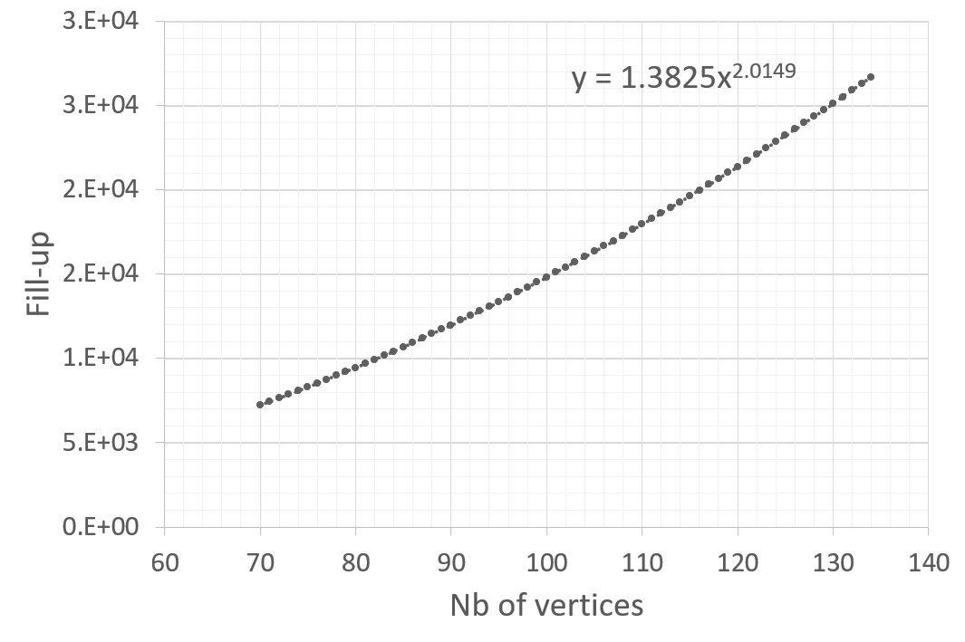
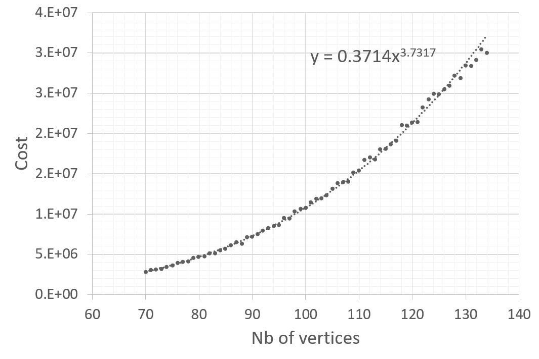
Figure 3: Average fill-up (left) and cost (right) for the reduction of the Vietoris–Rips filtration of a random point set sampled uniformly in $[0,1]^{2}$. The regression coefficients are shown in the figure.

Figure 4 shows the results for Erdős–Rényi filtrations. The regression yields an observed complexity of around $O(n^{2.08})$ for the fill-up and $O(n^{5.07})$ for the cost, which are quite far from our upper bounds of $O(n^{3}\log n)$ and $O(n^{6}\log n)$, respectively. Note that in the proof of Lemma 3.3, we assume that all columns with a pivot smaller than the threshold $T$ are dense, and we use the rather large value of $T=\Theta(\sqrt{n^{3}\log n})$ in the proof of Main Theorem 1. We speculate that a tighter bound has to analyze the behavior in this “subcritical regime” more carefully (a possible approach for that might be to use techniques from [order_pivoting] to find a probabilistic bound on the density of the columns). On the other hand, it is perhaps surprising that the empirical cost seems bigger than the empirical fill-up by a factor very close to $n^{3}$. That suggests that, unlike in the Vietoris–Rips case, Lemma 2.1 is not too pessimistic in bounding the cost of the reduction in this case.

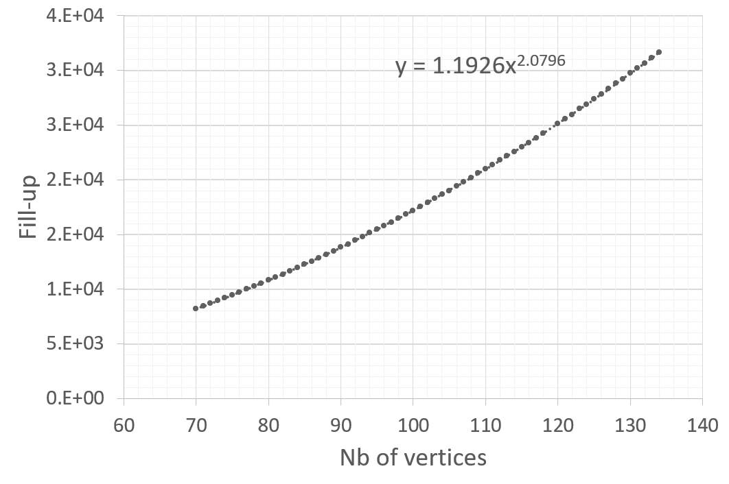
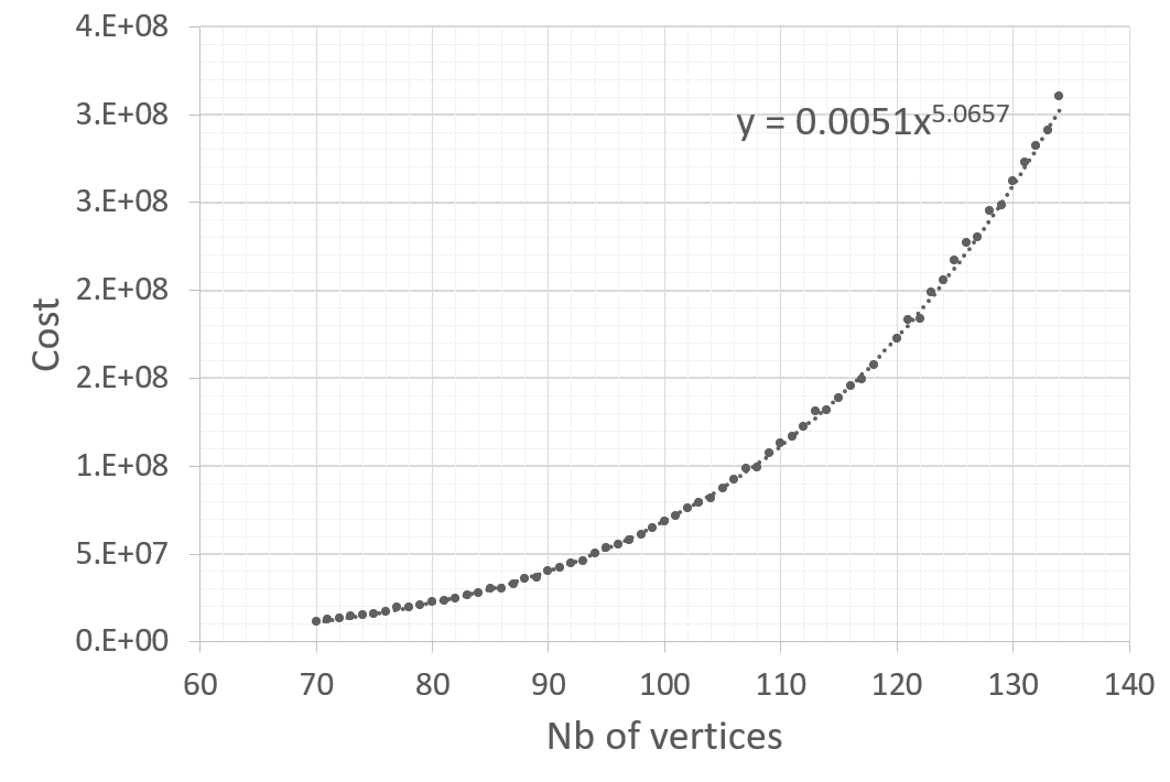
Figure 4: Average fill-up (left) and cost (right) for the reduction of the Erdős–Rényi filtration. The regression coefficients are shown in the figure.

7 Worst-case fill-up and complexity

Our upper bounds on average fill-up and cost are smaller than the respective worst-case estimates. However, these estimate are based on the assumption that the reduction algorithm produces dense columns (since the fill-up of a column with pivot $i$ is upper bounded with $i$). Since the boundary matrix initially has only a constant number of non-zero entries per column, the question is whether such a bound is really achieved in an example, or whether the upper bound is not tight.

Even for general boundary matrices of simplicial complexes, it requires some care to generate just one dense column in the reduced matrix. For the worst-case, however, one has to generate many such columns (to achieve the worst-case fill-up), and ensure that these columns get used in the reduction of subsequent columns (to achieve the worst-case cost). This has been done by Morozov [morozov2005persistence] for general simplicial complexes. However, restricting to clique complexes puts additional constraints and invalidates his example. In this section we show the following result:

Theorem 7.1.

For every $n$, there is a clique filtration over $n$ vertices, for which the left-to-right reduction of the $1$-boundary matrix has a fill-up of $\Theta(n^{4})$ and a cost of $\Theta(n^{7})$.

This result complements Main Theorem 1 because the clique filtration we construct is a possible instance of the ER filtration model, hence the expected fill-up and cost for this model are indeed smaller than the worst-case by a factor of roughly $n$.

Idea of the construction.

Recall that a clique filtration is not completely fixed by the order of edges: many triangles can be created by the insertion of an edge, forming columns in the boundary matrix with the same pivot, and the order of these columns influences the resulting matrix (even if their order was irrelevant for the expected bounds). Our construction for Theorem 7.1 carefully chooses an edge order and an order of the columns with the same pivot. The details are rather technical, so we start with a more high-level description of the major gadgets of our construction.

The main idea is to define two groups of $\Theta(n^{2})$ edges, or equivalently, rows of the boundary matrix that we call group II rows and group III rows, with group II rows having smaller index than group III rows (the notation is chosen to fit the technical description that follows). We first make sure to produce $\Theta(n^{2})$ columns in the reduced matrix such that each column has exactly one non-zero group III element that is its pivot, and $\Theta(n^{2})$ non-zero group II elements. We call such columns fat for now. Achieving this already yields a fill-up of $\Theta(n^{4})$. To get the cost bound, we make sure to produce $\Theta(n^{3})$ further columns (i.e., on the right of the fat columns) which we call costly columns. They have the property that during the reduction, they reach an intermediate state where they have gathered $\Theta(n^{2})$ non-zero elements in group III and their pivot is in this group as well. To complete the reduction, the algorithm is than required to add $\Theta(n^{2})$ fat columns to the current column. That means that the cost of reducing a costly column is $\Theta(n^{4})$, and since there are $\Theta(n^{3})$ costly columns, the bound on the cost follows.

$\begin{array}[]{|ccccc|cccccccc|ccccc|cccccc|ccccc}\lx@intercol\hfil\text{\footnotesize{Cascade 1}}\hfil\lx@intercol&&&&&&&&&\lx@intercol\hfil\text{\footnotesize{Cascade 2}}\hfil\lx@intercol\\ &&&&&&&&&&&&&&&&&&&&&&&\\ \cline{1-24}\cr\hbox{\pagecolor{black}}\hfil&&&&&&&&&&&&&&&&&&&&&&\hbox{\pagecolor{black}}\hfil&&\\ &&&&\hbox{\pagecolor{black}}\hfil&&&&&&&&&&&&&&&&\hbox{\pagecolor{black}}\hfil&&&{\color[rgb]{1,1,1}a}&{\color[rgb]{1,1,1}a}&{\color[rgb]{1,1,1}a}&&\hbox{\multirowsetup\large{II}}\\ &\hbox{\pagecolor{black}}\hfil&&&&&&&&&&&&&&&&&&&&&&\\ &&&\hbox{\pagecolor{black}}\hfil&&&&&&&&&&&&&&&&\hbox{\pagecolor{black}}\hfil&&&&\\ &&\hbox{\pagecolor{black}}\hfil&&&&&&&&&&&&&&&&&&&&&\hbox{\pagecolor{black}}\hfil\\ \cline{1-24}\cr&&&&&&&&&\hbox{\pagecolor{black}}\hfil&&&&\hbox{\pagecolor{black}}\hfil&&&&&&&&&&\\ &&&&&&&\hbox{\pagecolor{black}}\hfil&&&&&&&&&\hbox{\pagecolor{black}}\hfil&&&\hbox{\pagecolor{black}}\hfil&&&&{\color[rgb]{1,1,1}a}&{\color[rgb]{1,1,1}a}&{\color[rgb]{1,1,1}a}&&\hbox{\multirowsetup\large{III}}\\ &&&&&&\hbox{\pagecolor{black}}\hfil&&&&&&&&\hbox{\pagecolor{black}}\hfil&&&&&&&&&\hbox{\pagecolor{black}}\hfil\\ &&&&&&&&&&&\hbox{\pagecolor{black}}\hfil&&&&&&\hbox{\pagecolor{black}}\hfil&&&&&\hbox{\pagecolor{black}}\hfil&\\ &&&&&&&&&&&&\hbox{\pagecolor{black}}\hfil&&&\hbox{\pagecolor{black}}\hfil&&&&&\hbox{\pagecolor{black}}\hfil&&&\\ \cline{1-24}\cr\hbox{\pagecolor{black}}\hfil&\hbox{\pagecolor{black}}\hfil&&&&&&&&&&&\hbox{\pagecolor{black}}\hfil&&&&&&&&&&&\\ &\hbox{\pagecolor{black}}\hfil&\hbox{\pagecolor{black}}\hfil&&&&&&&&&\hbox{\pagecolor{black}}\hfil&&&&&&&&&&&&{\color[rgb]{1,1,1}a}&{\color[rgb]{1,1,1}a}&{\color[rgb]{1,1,1}a}&&\hbox{\multirowsetup\large{IV}}\\ &&\hbox{\pagecolor{black}}\hfil&\hbox{\pagecolor{black}}\hfil&&&&&&\hbox{\pagecolor{black}}\hfil&&&&&&&&&&&&&&\\ &&&\hbox{\pagecolor{black}}\hfil&\hbox{\pagecolor{black}}\hfil&&&\hbox{\pagecolor{black}}\hfil&&&&&&&&&&&&&&&&\\ &&&&\hbox{\pagecolor{black}}\hfil&&\hbox{\pagecolor{black}}\hfil&&&&&&&\hbox{\pagecolor{black}}\hfil&&&&&&&&&&\\ \cline{1-24}\cr&&&&&\hbox{\pagecolor{black}}\hfil&\hbox{\pagecolor{black}}\hfil&\hbox{\pagecolor{black}}\hfil&&&&&&&&&&&&&&&&{\color[rgb]{1,1,1}a}&{\color[rgb]{1,1,1}a}&{\color[rgb]{1,1,1}a}&&\hbox{\multirowsetup\large{V}}\\ &&&&&&&&\hbox{\pagecolor{black}}\hfil&\hbox{\pagecolor{black}}\hfil&&&&&&&&&&&&&&\\ &&&&&&&&&&\hbox{\pagecolor{black}}\hfil&\hbox{\pagecolor{black}}\hfil&\hbox{\pagecolor{black}}\hfil&&&&&&&&&&&\\ \cline{1-24}\cr&&&&&&&&&&&&&\hbox{\pagecolor{black}}\hfil&\hbox{\pagecolor{black}}\hfil&&&&&&&&&\\ &&&&&&&&&&&&&&\hbox{\pagecolor{black}}\hfil&\hbox{\pagecolor{black}}\hfil&&&&&&&&{\color[rgb]{1,1,1}a}&{\color[rgb]{1,1,1}a}&{\color[rgb]{1,1,1}a}&&\hbox{\multirowsetup\large{VI}}\\ &&&&&&&&&&&&&&&\hbox{\pagecolor{black}}\hfil&\hbox{\pagecolor{black}}\hfil&&&&&&&\\ &&&&&&&&&&&&&&&&\hbox{\pagecolor{black}}\hfil&\hbox{\pagecolor{black}}\hfil&&&&\hbox{\pagecolor{black}}\hfil&&\\ &&&&&&&&&&&&&&&&&\hbox{\pagecolor{black}}\hfil&\hbox{\pagecolor{black}}\hfil&&&&&\\ \cline{1-24}\cr&&&&&&&&&&&&&&&&&&\hbox{\pagecolor{black}}\hfil&\hbox{\pagecolor{black}}\hfil&\hbox{\pagecolor{black}}\hfil&&&{\color[rgb]{1,1,1}a}&{\color[rgb]{1,1,1}a}&{\color[rgb]{1,1,1}a}&&\hbox{\multirowsetup\large{VII}}\\ &&&&&&&&&&&&&&&&&&&&&\hbox{\pagecolor{black}}\hfil&\hbox{\pagecolor{black}}\hfil&\hbox{\pagecolor{black}}\hfil\\ \cline{1-24}\cr\end{array}$

$\begin{array}[]{|ccccc|cccccccc|ccccc|cccccc|}&&&&&\lx@intercol\hfil\text{\footnotesize{Fat col.}}\hfil\lx@intercol&&&&&&\lx@intercol\hfil\text{\footnotesize{Costly col.}}\hfil\lx@intercol\\ &&&&&&&&&&&&&&&&&&&&&&&\\ \hline\cr\hbox{\pagecolor{black}}\hfil&&&&&&\hbox{\pagecolor{black}}\hfil&\hbox{\pagecolor{black}}\hfil&&\hbox{\pagecolor{black}}\hfil&&\hbox{\pagecolor{black}}\hfil&\hbox{\pagecolor{black}}\hfil&&&&&&&&&&\hbox{\pagecolor{black}}\hfil&\\ &&&&\hbox{\pagecolor{black}}\hfil&&\hbox{\pagecolor{black}}\hfil&\hbox{\pagecolor{black}}\hfil&&\hbox{\pagecolor{black}}\hfil&&\hbox{\pagecolor{black}}\hfil&\hbox{\pagecolor{black}}\hfil&&&&&&&&&&&\\ &\hbox{\pagecolor{black}}\hfil&&&&&\hbox{\pagecolor{black}}\hfil&\hbox{\pagecolor{black}}\hfil&&\hbox{\pagecolor{black}}\hfil&&\hbox{\pagecolor{black}}\hfil&\hbox{\pagecolor{black}}\hfil&&&&&&&&&&&\\ &&&\hbox{\pagecolor{black}}\hfil&&&\hbox{\pagecolor{black}}\hfil&\hbox{\pagecolor{black}}\hfil&&\hbox{\pagecolor{black}}\hfil&&\hbox{\pagecolor{black}}\hfil&\hbox{\pagecolor{black}}\hfil&&&&&&&\hbox{\pagecolor{black}}\hfil&&&&\\ &&\hbox{\pagecolor{black}}\hfil&&&&\hbox{\pagecolor{black}}\hfil&\hbox{\pagecolor{black}}\hfil&&\hbox{\pagecolor{black}}\hfil&&\hbox{\pagecolor{black}}\hfil&\hbox{\pagecolor{black}}\hfil&&&&&&&&&&&\hbox{\pagecolor{black}}\hfil\\ \hline\cr&&&&&&&&&\hbox{\pagecolor{black}}\hfil&&&&\hbox{\pagecolor{black}}\hfil&&&&&&\hbox{\pagecolor{black}}\hfil&\hbox{\pagecolor{black}}\hfil&&\hbox{\pagecolor{black}}\hfil&\hbox{\pagecolor{black}}\hfil\\ &&&&&&&\hbox{\pagecolor{black}}\hfil&&&&&&&&&\hbox{\pagecolor{black}}\hfil&&&\hbox{\pagecolor{black}}\hfil&\hbox{\pagecolor{black}}\hfil&&\hbox{\pagecolor{black}}\hfil&\hbox{\pagecolor{black}}\hfil\\ &&&&&&\hbox{\pagecolor{black}}\hfil&&&&&&&&\hbox{\pagecolor{black}}\hfil&&&&&\hbox{\pagecolor{black}}\hfil&\hbox{\pagecolor{black}}\hfil&&\hbox{\pagecolor{black}}\hfil&\hbox{\pagecolor{black}}\hfil\\ &&&&&&&&&&&\hbox{\pagecolor{black}}\hfil&&&&&&\hbox{\pagecolor{black}}\hfil&&\hbox{\pagecolor{black}}\hfil&\hbox{\pagecolor{black}}\hfil&&\hbox{\pagecolor{black}}\hfil&\hbox{\pagecolor{black}}\hfil\\ &&&&&&&&&&&&\hbox{\pagecolor{black}}\hfil&&&\hbox{\pagecolor{black}}\hfil&&&&\hbox{\pagecolor{black}}\hfil&\hbox{\pagecolor{black}}\hfil&&\hbox{\pagecolor{black}}\hfil&\hbox{\pagecolor{black}}\hfil\\ \hline\cr\hbox{\pagecolor{black}}\hfil&\hbox{\pagecolor{black}}\hfil&&&&&&&&&&&\hbox{\pagecolor{black}}\hfil&&&&&&&&&&&\\ &\hbox{\pagecolor{black}}\hfil&\hbox{\pagecolor{black}}\hfil&&&&&&&&&\hbox{\pagecolor{black}}\hfil&&&&&&&&&&&&\\ &&\hbox{\pagecolor{black}}\hfil&\hbox{\pagecolor{black}}\hfil&&&&&&\hbox{\pagecolor{black}}\hfil&&&&&&&&&&&&&&\\ &&&\hbox{\pagecolor{black}}\hfil&\hbox{\pagecolor{black}}\hfil&&&\hbox{\pagecolor{black}}\hfil&&&&&&&&&&&&&&&&\\ &&&&\hbox{\pagecolor{black}}\hfil&&\hbox{\pagecolor{black}}\hfil&&&&&&&\hbox{\pagecolor{black}}\hfil&&&&&&&&&&\\ \hline\cr&&&&&\hbox{\pagecolor{black}}\hfil&\hbox{\pagecolor{black}}\hfil&\hbox{\pagecolor{black}}\hfil&&&&&&&&&&&&&&&&\\ &&&&&&&&\hbox{\pagecolor{black}}\hfil&\hbox{\pagecolor{black}}\hfil&&&&&&&&&&&&&&\\ &&&&&&&&&&\hbox{\pagecolor{black}}\hfil&\hbox{\pagecolor{black}}\hfil&\hbox{\pagecolor{black}}\hfil&&&&&&&&&&&\\ \hline\cr&&&&&&&&&&&&&\hbox{\pagecolor{black}}\hfil&\hbox{\pagecolor{black}}\hfil&&&&&&&&&\\ &&&&&&&&&&&&&&\hbox{\pagecolor{black}}\hfil&\hbox{\pagecolor{black}}\hfil&&&&&&&&\\ &&&&&&&&&&&&&&&\hbox{\pagecolor{black}}\hfil&\hbox{\pagecolor{black}}\hfil&&&&&&&\\ &&&&&&&&&&&&&&&&\hbox{\pagecolor{black}}\hfil&\hbox{\pagecolor{black}}\hfil&&&&\hbox{\pagecolor{black}}\hfil&&\\ &&&&&&&&&&&&&&&&&\hbox{\pagecolor{black}}\hfil&\hbox{\pagecolor{black}}\hfil&&&&&\\ \hline\cr&&&&&&&&&&&&&&&&&&\hbox{\pagecolor{black}}\hfil&\hbox{\pagecolor{black}}\hfil&\hbox{\pagecolor{black}}\hfil&&&\\ &&&&&&&&&&&&&&&&&&&&&\hbox{\pagecolor{black}}\hfil&\hbox{\pagecolor{black}}\hfil&\hbox{\pagecolor{black}}\hfil\\ \hline\cr\end{array}$

Figure 5: Example of a boundary matrix realising the worst-cases, unreduced (left) and halfway in the reduction (right), i.e. after running through both cascades.

The main question is: how do we produce fat and costly columns? Let us start with fat columns. The key notion is the one of the cascade; we refer to Figure 5 for an illustration of the following description. We introduce another set of $\Theta(n^{2})$ edges that define group IV (which come after group III in the edge order). Let $i$ denote the row index of some group IV row. Our construction ensures that there is a column with pivot $i$ that has as further entries $i-1$ and some entry in group II. We select this column as step column for $i$, so it does not change in the reduction. The set of these step columns forms the cascade. Moreover, we ensure that all entries in group II over all cascade columns are at pairwise distinct indices to avoid unwanted cancellation in later steps.

After construction the cascade, we include $\Theta(n)$ edges of group V. This generates $\Theta(n^{2})$ columns that acquire a group IV pivot during the reduction. Moreover, we ensure that the (partially reduced) column has exactly one non-zero element of group III, and that all these group III indices are pairwise distinct for all columns in this group. To reduce this column further, we have to add the cascade columns, until the non-zero group III element becomes the pivot. While iterating through the cascade, the reduced column accumulates more and more non-zero elements in group II, resulting in a size of $\Theta(n^{2})$. This creates the fat columns. Note that no two fat columns are added to each other because we ensure that they have pairwise distinct pivots from group III – again, this avoids unwanted cancellation.

For generating costly columns, the idea is the same: we construct another cascade (using rows of group VI) and then a group VII to ensure that the cascade will fill up columns in the row indices of group III. Afterwards, the reduction has to continue and adds columns with pivots at group III, which are precisely the fat columns from the previous step.

Figure 6: Points of the five groups, where the point $x_{i}$ belong to the group $X$, and edges of the first five groups. The edges of group I and II are thicker, the ones of group V are dashed.

7.2.

Groups of edges. Group I is given by the $3p$ edges between $roof$ and $A$, $roof$ and $B$, and $roof$ and $E$, by the $2(p-1)$ edges that form the path $(a_{0},\dots,a_{p-1})$ in $A$ and the path $(e_{0},\dots,e_{p-1})$ in $E$, by the edges $a_{0}c_{0}$ and $b_{p-1}e_{0}$, and finally by the $\frac{1}{2}(p^{2}+p)$ edges between the last $\frac{p+1}{2}$ vertices in $E$ and all the vertices in $D$. Group II has $p(p-1)$ edges, given by all the edges of the complete bipartite graph between $C$ and $D$ but for the edges $c_{i}d_{i}$, for $i=0,\dots,p-1$. Group III is given by all the $p^{2}$ edges that form a complete bipartite graph between $B$ and $C$. The order of the edges inside each of these groups is irrelevant and chosen randomly. The groups IV and VI are given by a subset of cardinality $p^{2}-1$ of the $2p^{2}$ edges between $A$ and $C\cup D$, and between $E$ and $B\cup C$, respectively. These edges and their order have to be chosen carefully and we describe them in Paragraphs 7.3 and LABEL:P:order_edges_VI, respectively. Group V is given by all the $p$ edges from $a_{p-1}$ to $B$. Group VII is made of the $\frac{(p+1)p}{2}$ edges between $\{b_{\frac{p-1}{2}},\dots,b_{p-1}\}$ and $D$, and are ordered firstly in decreasing order on the indices in $B$ and then in decreasing order on the indices in $D$. Finally, the eighth group is given by all the remaining edges, whose order is irrelevant as long as they enter in the filtration after all the previous groups. We do not consider them further. The first five groups are depicted in Figure 6 and the sixth and seventh groups in the zoom-in of Figure 7.

Figure 7: Zoom-in to the edges of groups VI and VII. For readability, $j=\frac{p-1}{2}$. The edges of group VII are thicker.

7.3.

Group IV. Since each vertex in the graph $G=(C\cup D,\text{group II})$ has even degree, there exists an Eulerian path on $G$, starting in $c_{0}$. The edges in group IV are given as follows: for $j=1,\dots,p-1$, starting from the $(jp-j)$-th vertex in the path, we connect $p-1$ consecutive vertices of the Eulerian path to the vertex $a_{j-1}$. The edges are ordered first by increasing $j$ and then by the order of the Eulerian path. Note that, by construction, none of the columns with pivots in row group IV have a non-zero element in row group III.

We choose as step columns the triangles with two edges in group IV, i.e., the elements in the cascade. Of these triangles, all but $p-1$, i.e., the triangles constructed using the edges between elements in $A$, have as third edge an element of the Eulerian path. In particular, we have $(p-1)^{2}$ step columns that have all different elements in the row group II. These columns form the first cascade. The order of the non-step triangles is irrelevant.