Testing the monocentric standard urban model in a global sample of cities

Abstract

Using a unique dataset containing gridded data on population densities, rents, housing sizes, and transportation in 192 cities worldwide, we investigate the empirical relevance of the monocentric standard urban model (SUM). Overall, the SUM seems surprisingly capable of capturing the inner structure of cities, both in developed and developing countries. As expected, cities spread out when they are richer, more populated, and when transportation or farmland is cheaper. Respectively 100% and 87% of the cities exhibit the expected negative density and rent gradients: on average, a 1% decrease in income net of transportation costs leads to a 21% decrease in densities and a 3% decrease in rents per m². We also investigate the heterogeneity between cities of different characteristics in terms of monocentricity, informality, and amenities.

Accepted manuscript in Regional Science and Urban economics on August 11th, 2022.

1 Introduction

Understanding urbanization patterns and modeling urban dynamics have been a subject of research for at least a century (Duranton and Puga, 2015). These questions have recently been brought back into the spotlight in the context of current environmental crises, as urban sprawl is a key driver of both climate change (IPCC, 2014) and biodiversity losses (IPBES, 2019; Seto et al., 2012).

A well-established framework to tackle these issues is the Standard Urban Model (SUM), widely used in theoretical and applied papers (Brueckner, 2001). The SUM, initially developed by Alonso (1964), Muth (1969), and Mills (1967), describes the relationship between land use, land value, and transportation costs in cities, and relies on the following mechanisms. Households trade off between housing size and transportation costs to employment centers, which, in a monocentric city, results in high bid-rents in city centers, where transportation costs are low, and low bid-rents in peripheries. Under the assumption of competitive land markets, private developers will provide a high housing supply in city centers and a low housing supply in peripheries, as inelastically supplied land and diminishing returns to factor inputs imply that taller buildings require higher floor space rents (Ahlfeldt and Barr, 2022). From these mechanisms, aggregated results can be derived at the city level. Wheaton (1974) showed that, under the assumptions of monocentricity and monetary commuting costs, large populations and high incomes lead to larger urbanized areas, while high transportation costs and high agricultural land prices lead to smaller urban areas.

An extensive literature investigates the validity of the SUM and empirically examines its main conclusions in terms of population densities, rents, and urbanized areas, with studies on density gradients starting even before the theory was formulated (Clark, 1951). However, this literature still suffers from some limitations. First, few studies simultaneously investigate the model’s predictions in terms of urbanized areas, population densities, and rent gradients in relation to transportation costs within cities. Indeed, while the literature on density gradients in cities is well developed (see, for instance, the review by McDonald, 1989), the literature on dwelling rents or prices is less developed due to data limitations, and most studies focus on one or two cities, preventing comparison between cities or generalization of results (Duranton and Puga, 2015; McMillen, 2006, 2010). In addition, most of the existing studies investigate developed countries. Exceptions include Deng et al. (2008), Ke et al. (2009), Angel et al. (2011), and Jedwab et al. (2021) for urbanized area sizes. Exceptions regarding density gradients are more numerous as the literature is larger but include only three large-scale studies comparing a large number of cities (Bertaud and Malpezzi, 2014; Mills and Tan, 1980; Ingram and Carroll, 1981) and a few single case studies, mainly in China (Chen, 2010; Feng et al., 2009; Wang and Zhou, 1999).

However, the recent increase in data availability offers an opportunity to deepen our understanding of urban forms and city structures globally. Satellite data can be used to compare urban shapes: for instance, Harari (2020) uses such data to demonstrate the impact of city compactness on accessibility and welfare. New datasets, such as night lights (Henderson et al., 2012) and Twitter data (Indaco, 2020) can also be used as proxies for economic activity at a disaggregated, e.g. city, level. Regarding transportation, big datasets, for instance from Google Maps, allow detailed analysis of mobility and congestion for large samples of cities (Akbar et al., 2018; Hanna et al., 2017).

Using spatially-explicit data on population densities, rents, dwelling sizes, land cover, and transport time in 192 cities across all continents, this paper empirically assesses the ability of the SUM to represent cities throughout the world. We show that the SUM captures urban structures surprisingly well, both in developed and developing countries, with most cities exhibiting the expected negative rent and density gradients: on average, a 1% decrease in income net of transportation costs leads to a 21% decrease in densities and a 3% decrease in rents per m², and moving 1km farther from the city center decreases rents by 1.4% and population density by 8.5%. We structurally estimate that the median capital elasticity of housing production over the sample of cities is 0.87, and that the median percentage of housing expenses in households’ income net of transportation costs is 33%. Our sample also allows us to investigate heterogeneity between cities: we show that polycentricity, informality, and local amenities weaken the relationship between rents or densities and incomes net of transportation costs, flattening density and rent gradients in cities. Aggregated predictions of the model in terms of urbanized areas are also verified in our sample: cities spread out more when they are richer, more populated, and when transportation or famland rents are less costly.

The remainder of the paper is organized as follows. Section 2 introduces the monocentric SUM and the extant evidence regarding its main predictions. Section 3 presents the data. Section 4 empirically tests the three main relationships derived from the model, and section 5 discusses the results.

2 Introducing the monocentric city model

2.1 Theory

This section describes the SUM of urban economics and derives expressions for three endogenous variables (rents within cities, population densities, and total urbanized area of each city) as a function of a set of exogenous variables (population, farmland rents, income, per-distance transport cost). We analyse a sample of cities indexed by c, with locations within cities indexed by i, in a closed-city framework assuming exogenous populations.

In the first step, we derive dwellings’ bid-rents per m² at location i in city c, denoted $R_{i,c}$, as a function of transportation costs to the city center (where we assume for simplicity that all jobs are located) $T_{i,c}$ using the spatial equilibrium condition. We assume that households seek to maximise their Cobb-Douglas utilities:

$$max\hskip 8.53581ptU(z_{i,c},\,q_{i,c})=z_{i,c}^{\alpha_{c}}\,q_{i,c}^{\beta_{c}}\hskip 85.35826pts.t.\hskip 8.53581ptz_{i,c}+q_{i,c}R_{i,c}+T_{i,c}\leq Y_{c}$$ (1)

with $q_{i,c}$ the size of the dwellings in pixel i and city c, $Y_{c}$ the income in city c (assumed as constant over the city), $z_{i,c}$ the consumption of a composite good (whose price is normalized to 1), and $\alpha_{c}$ and $\beta_{c}$ the Cobb-Douglas parameters (such that $\alpha_{c}+\beta_{c}=1$).

From equation 1, we find that:

$$\begin{array}[]{l}q_{i,c}=\beta_{c}(Y_{c}-T_{i,c})/R_{i,c}\\ z_{i,c}=\alpha_{c}(Y_{c}-T_{i,c})\end{array}$$ (2)

Using the spatial equilibrium condition and writing $u_{c}$ the uniform utility at equilibrium, we find:

$$R_{i,c}=R_{0,c}\,\frac{(Y_{c}-T_{i,c})^{1/\beta_{c}}}{Y_{c}^{1/\beta_{c}}}\hskip 28.45274pt\text{with}\hskip 28.45274ptR_{0,c}=(\frac{\alpha_{c}^{\alpha_{c}}\,\beta_{c}^{\beta_{c}}\,Y_{c}}{u_{c}})^{1/\beta_{c}}$$ (3)

In the second step, we derive population density as a function of transportation costs. We assume that absentee private developers produce housing from capital $K_{i,c}$ and urbanizable land $L_{i,c}$ with the following Cobb-Douglas production function, with the parameters $A_{c}$, $a_{c}$ and $b_{c}$ such that $a_{c}+b_{c}=1$ :

$$H(K_{i,c},\,L_{i,c})=A_{c}\,L_{i,c}^{a_{c}}\,K_{i,c}^{b_{c}}$$ (4)

With $k_{i,c}=K_{i,c}/L_{i,c}$ (capital intensity per urbanizable land surface area) and $h=H/L_{i,c}$ (housing density, i.e. number of m2 built upon per m2 of available ground), equation 4 can be rewritten:

$$h(k_{i,c})=A_{c}k_{i,c}^{b_{c}}$$ (5)

Developers seek to maximize their profit per land surface area $\pi_{i,c}=R_{i,c}h(k_{i,c})-\rho k_{i,c}$ considering a capital cost $\rho$. Thus, housing supply is written:

$$H_{i,c}=A_{c}^{1/a_{c}}(b_{c}R_{i,c}/\rho)^{b_{c}/a_{c}}L_{i,c}$$ (6)

and total population per pixel $N_{i,c}$ is written:

$$N_{i,c}=H_{i,c}/q_{i,c}=A_{c}^{1/a_{c}}(b_{c}R_{i,c}/\rho)^{b_{c}/a_{c}}L_{i,c}/q_{i,c}$$ (7)

Replacing $q_{i,c}$ by its expression in equation 2:

$$N_{i,c}=A_{c}^{1/a_{c}}(b_{c}/\rho)^{b_{c}/a_{c}}L_{i,c}R_{i,c}^{1/a_{c}}\frac{1}{\beta_{c}(Y_{c}-T_{i,c})}$$ (8)

The population density per pixel $n_{i,c}=N_{i,c}/L_{i,c}$ can be expressed as:

$$n_{i,c}=A_{c}^{1/a_{c}}(b_{c}/\rho)^{b_{c}/a_{c}}R_{i,c}^{1/a_{c}}\frac{1}{\beta_{c}(Y_{c}-T_{i,c})}$$ (9)

Finally, replacing $R_{i,c}$ by its expression in equation 3:

$$n_{i,c}=A_{c}^{1/a_{c}}(\frac{b_{c}}{\rho})^{b_{c}/a_{c}}(\frac{\alpha_{c}^{\alpha_{c}}}{u})^{1/(\beta_{c}a_{c})}\beta_{c}^{b_{c}/a_{c}}(Y_{c}-T_{i,c})^{(1-\beta_{c}a_{c})/\beta_{c}a_{c}}$$ (10)

In the third step, we want to derive the total urban area as a function of city characteristics. We assume for simplicity that the city is circular, i.e. that the amount of urbanizable land per pixel is constant, with $L_{i,c}=1$, and that transportation cost can be broken down as $T_{i,c}=d_{i,c}t_{c}$ with $d_{i,c}$ the distance from pixel i to the city center of city c and $t_{c}$ the constant per unit transportation cost.

We assume the following equilibrium conditions:

• from equation 3, we find that bid-rents decrease from city centers to peripheries. We assume that the bid-rent $R_{i,c}$ intersects with farmland rent $\overline{R}_{c}$ at the fringe of the city $\overline{d}_{c}$ and at a transport cost $\overline{T}_{c}=\overline{d}_{c}t_{c}$, such that:

$$\overline{R}_{c}=R_{0,c}\,(1-\frac{\overline{T}_{c}}{Y_{c}})^{1/\beta_{c}}=R_{0,c}\,(1-\frac{t_{c}\overline{d}_{c}}{Y_{c}})^{1/\beta_{c}}$$ (11)

• in a closed-city model, all the population of the city $N^{*}$ lives within the city, i.e.

$$N_{c}^{*}=\int{}^{i}n_{i,c}di$$ (12)

Brueckner (1987, pp. 830-836 and 840-844) shows that, under the following hypotheses:

• preference of households for housing and composite good is represented by a quasi-concave utility function, as in equation 1;

• housing supply is represented by a concave production function with constant returns, as in equation 4;

we can derive the following relationships:

$$\frac{\text{$\partial$}\overline{d}_{c}}{\partial N_{c}^{*}}>0,\frac{\text{$\partial$}\overline{d}_{c}}{\text{$\partial$}Y_{c}}>0,\frac{\text{$\partial$}\overline{d}_{c}}{\text{$\partial$}t_{c}}<0,\frac{\text{$\partial$}\overline{d}_{c}}{\text{$\partial$}\overline{R}_{c}}<0,$$ (13)

Therefore, urban areas are expected to decrease with transportation cost per unit of distance and farmland rent and increase with total population and income.

2.2 Extant evidence

This section reviews the extant literature and evidence regarding the three relationships derived from the SUM in the previous subsection: bid-rents expressed as a function of transportation costs (equation 3), population density as a function of transportation costs (equation 10), and urbanized area as a function of the total population, the average income, transportation costs, and farmland rents (equation 13).

2.2.1 Rent gradients

Studies beginning as far back as the 1970s have measured rent or land price gradients within cities. Most of them have found evidence of negative rent or land price gradients from city centers to the suburbs, mainly in the US (Coulson, 1991) and the UK (Cheshire and Sheppard, 1995), and more recently in Berlin (Ahlfeldt, 2011).

Nevertheless, flat or inverted rent or land price gradients have been measured in some cities. For instance, Yinger (1979) found the expected negative rent gradients in Madison, in the USA, but not in the more polycentric setting of St Louis. Working on Chicago, McDonald and Bowman (1979) found a negative land price gradient close to the Central Business District (CBD) but an inverted land price gradient farther away, which they explained by polycentrism, racial segregation, or disamenities such as air pollution or congestion in the city center. Also in Chicago, McMillen (1996) showed that the distance to the CBD could satisfactorily explain land values in the city between 1836 and 1928, but that it was no longer significant after 1960, as the development of O’Hare Airport made the city more polycentric.

Beyond accessibility, other variables have been shown to impact rents or land values, modifying the gradient. Cheshire and Sheppard (1995) found the expected negative land price gradient in Reading and Darlington, in the UK, but they use a fully hedonic model and show that, in addition to accessibility, location-specific and dwelling-specific amenities play a key role in determining rents. More recently, Ahlfeldt (2011) showed that the monocentric SUM performs satisfactorily if we account for structural and neighborhood characteristics such as distances to the nearest school or green space. He also showed that gravity employment accessibility measures perform better than the monocentric SUM in the polycentric setting of Berlin.

To summarize, despite the early literature on rent and land value gradients, the evidence for the negative relationship between rent and distance to CBD is mixed. Heterogeneity in rent gradients between cities can be explained by polycentricity (Yinger, 1979; McMillen, 1996) and location-based and dwelling-based amenities (Cheshire and Sheppard, 1995). A more systematic measure of rent gradients in various cities and an evaluation of the explanatory power of the hypotheses that have been proposed in the literature would usefully complement the existing studies.

2.2.2 Density gradients

The literature concerning population density gradients, summarized in McDonald (1989) and Duranton and Puga (2015), is wider, since data on population densities are easier to obtain than data on rents or land prices. An initial line of research, starting even before the formulation of the theory (Clark, 1951), sought to empirically find regularities in population densities. Many studies support the negative exponential function (Berry et al., 1963; Weiss, 1961), theoretically grounded in Muth (1961). However, other functions have been proposed in the literature, including the addition of a quadratic component to the negative exponential function to describe the population crater near the city center (Newling, 1969; Latham and Yeates, 1970), the inverse square function (Stewart and Warntz, 1958; Batty and Sik Kim, 1992), and the Gaussian function (Ingram, 1971; Guy, 1983). A full review of these functional forms can be found in Martori and Suriñach Caralt (2002), and Qiang et al. (2020) performed a recent assessment of their explanatory power on American cities. Overall, all these studies agree that population densities decrease from the city center to the periphery, potentially attenuated by the city center population density crater, due to the concentration of economic activities.

A second line of research has compared density gradients, either in the same city across time or between cities. Two main results emerge from this literature. First, there is evidence of a flattening of density gradients over time in Latin America (Ingram and Carroll, 1981) and the US (Mills, 1970; Macauley, 1985; Kim, 2007), which might be due to an increase in incomes and a decrease in transportation costs (Mills, 1970). Second, this gradient depends on the characteristics of the cities. More populous cities tend to have flatter gradients (Muth, 1969; Guest, 1973; Edmonston and Davies, 1976; Glickman and Oguri, 1978; Johnson and Kau, 1980; Mills and Tan, 1980; Alperovich, 1983; Bertaud and Malpezzi, 2014): one explanation is that employment subcenters are more likely to emerge in large areas. Older urban areas tend to have steeper gradients, possibly because of the inertia in urban shapes: cities that developed when transportation costs were high are more likely to be compact (see the studies by Glickman and Oguri, 1978, in Japan and Johnson and Kau, 1980, in the US). Overall, income has been found to have a weak negative impact on the steepness of the gradient (Mills and Tan, 1980). Comparing developed and developing countries, Mills and Tan (1980) found that developed countries have flatter density functions than developing countries, as they have higher incomes and better urban transportation systems. Working on a diverse sample of 57 cities, Bertaud and Malpezzi (2014) found that cities subject to stringent regulations, such as Brasilia, or complex geographies, such as coastal cities, exhibit a flatter gradient.

Recently, the increase in data availability has allowed studies to be performed on large samples of cities (see for instance Lemoy and Caruso, 2020, working on 300 European cities) or with better proxies for transportation costs. Qiang et al. (2020), for instance, use transportation time data from Google Maps instead of distances to city centers. These data could allow empirical assessment, using larger samples and with increased accuracy, of the extant results relating to density gradient heterogeneity between cities of different sizes or degrees of monocentricity found in the literature.

2.2.3 Urban areas

Finally, the following relationship can be derived from the SUM with respect to urban areas: their sizes should depend positively on population and income and negatively on transportation costs and farmland rents (equation 13). Many papers have empirically verified these results in the US (Brueckner and Fansler, 1983; McGrath, 2005; Wassmer, 2006; Spivey, 2008; Paulsen, 2012), finding that population, income, and farmland rents have the expected impact on urban areas. An important exception is Spivey (2008), estimating a negative income elasticity, which she explains by the fact that the increase in incomes increases the demand for more affordable housing farther from the city center, but also raises the opportunity cost of time, the second effect outweighing the first. However, these studies struggled to find proxies for transportation costs, leading to mixed results. Spivey (2008) uses the fraction of households owning a car, which is not robust in her main specification, and the Texas Transportation Institute’s “time travel index” and “congestion cost index,” with which she finds mixed evidence. Paulsen (2012) does not include any commuting cost variables: the author considered the census average travel time to work, but finally dropped this variable.

Fewer studies exist in Europe. Oueslati et al. (2015) found conclusive results, with all variables being significant and of the expected sign. In particular, the authors found a high coefficient for farmland rents, which reflects the fact that in Europe, agriculture at the urban fringe is often highly intensive, offering relatively high yields and profits. In Germany, Schmidt et al. (2020) found a particularly low coefficient for income, which they explain by the fact that increased demand for housing is not realized due to growth management policies and restrictive land-use regulations. Their proxies for transportation costs were found to be unreliable, leading to insignificant estimates, or to estimates whose sign is opposite to that which is expected. They also found differences between east and west Germany and between growing and shrinking regions.

Few studies focused on developing countries. The existing studies on China (Deng et al., 2008; Ke et al., 2009) found that income growth played a significant role in determining urban sprawl. Recently, Jedwab et al. (2021) showed that cities in developing countries grow differently to those in developed countries, i.e. by crowding “in” instead of sprawling or growing “up”.

At a global level, analyzing both total urban land cover in 206 countries and urban land cover in 3646 large urban areas worldwide, Angel et al. (2011) found significant estimates of the expected sign, except for transportation costs. However, the authors do not analyze the heterogeneity of their results by world regions or development level.

3 Data

3.1 Spatially-explicit data

Our main dataset, described in detail in Lepetit et al. (2022), is a spatially-explicit dataset including population densities, rents, dwelling sizes, transportation times, and land cover in 192 cities worldwide. This dataset’s originality lies in the provision of data on cities’ internal structures at a 1km² resolution, in particular on rents and transportation times, while covering a large and diverse sample of 192 cities on five continents. By combining data on density, real estate, transportation, and land cover, this dataset allows us to run an integrated analysis of the validity of the SUM in the sample. The main data collection steps are summarized below.

The cities were chosen to obtain wide geographical coverage, and represent different cultural and historical backgrounds. However, data availability, in particular for real estate, has been a limiting criterion. The cities selected are medium to large cities: they all have more than 300,000 inhabitants, and together represent 800 million people, i.e. 19% of the global urban population, or 34% of the people living in cities of more than 300,000 inhabitants (Figure 1).

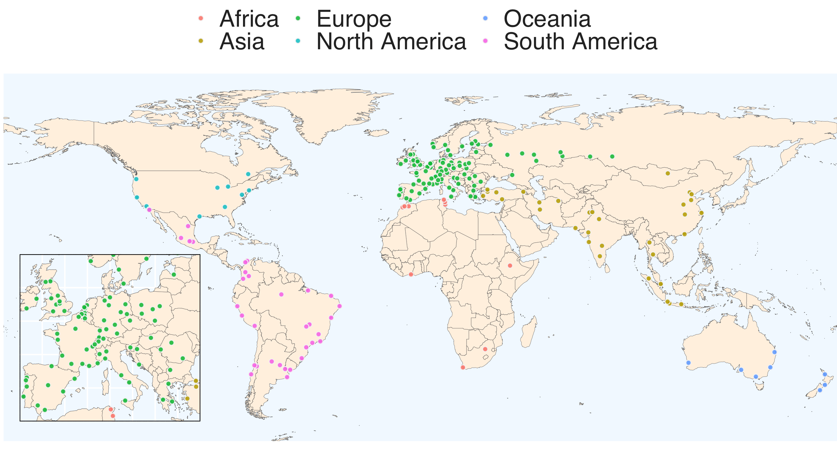
Figure 1: Sample of cities for which data were collected.

First, we divided each city into a georeferenced 1 km²- resolution grid encompassing the whole urban area. Then, we combined data from different sources and aggregated them on these grids. For land use, we used the European Space Agency land cover data (ESA, 2017), available worldwide at a 300m spatial resolution on an annual basis from 1992 to 2015. We reclassified areas as “urbanizable" (e.g., farmlands) or “non-urbanizable” (e.g., water bodies) (A). For population density, we used the European Commission GHSL data available for 1975, 1990, 2000, and 2015 at a 250m resolution worldwide (Schiavina et al., 2019).

Data on dwelling rents per m² and dwelling sizes were most difficult to obtain, as no global database exists. We obtained them by web-scraping real estate websites between 2017 and 2020. The websites were selected to meet four criteria: the website must have nationwide coverage to ensure consistent results in a given country, it must geolocalize the dwellings, have values for both rent or sale prices and dwelling size, and be written in the local language and give prices in local currency to limit real estate ads targeting expatriates. We aggregated the data at the grid cell level by taking mean rents per square meter. We computed two variables to assess rent data quality (Table 1): first, "Real estate data market cover" which corresponds to the average number of real estate ads that were scraped per grid cell in the city and second, "Real estate data spatial cover", the percentage of grid cells that have density data and for which we also have data on rents. In 109 cities out of 192, the spatial data cover of rent ads is above 10%, and in 153 cities out of 192, the spatial data cover is above 5%. In 95 cities out of 192, we scraped more than 1 rent ad per 1,000 inhabitants, and in 174 cities out of 192, we scraped more than 1 rent ad per 10,000 inhabitants.

	Mean	Min.	Q1	Med.	Q3	Max.	Nb. of obs.
Market cover	14168	98	550	1020	2281	810960	192
Spatial cover	11.81%	0.07%	5.79%	10.90%	15.41%	59.14%	192

Table 1: Real estate data quality.
For 50% of the cities, we scraped more than 1 real estate ad per 1,020 inhabitants, and we scraped real estate ads for more than 10.9% of the inhabited pixels.

Transport distances and durations from each grid cell to the city center have been estimated using Google Maps and Baidu Maps APIs (Application Programming Interfaces). Different definitions of city centers exist in the urban economics literature. Most rely on job density data, which are unfortunately not consistently available for the cities in the database. Therefore, this study defined city centers on the basis of a compromise between five qualitative criteria: the geographical center of the data, the historical center of the city, the location of the public transport hub, the official central business district, and the city hall location. When available, both driving and public transport data were collected for typical afternoon rush hours. It was not possible to collect transport data from each grid cell, so 10% of all cells were collected and then performed bivariate interpolation using the R package AKIMA, allowing us to approximate transportation times for the whole grid.

3.2 Aggregated data at the city level

To complement the spatially-explicit dataset, we use data relating to characteristics of the whole cities, detailed below.

City populations are derived from the spatially explicit dataset and correspond to the sum of the densities over the grid. Similarly, urbanized areas correspond to the sum of the urbanized area data over the grid. We are aware that this definition of city limits is likely to overestimate population and urbanized area, but it allows the extent of "urban area" to be identical for the two variables and independent of city administrative or legally-defined boundaries. Indeed, the extent of functional urban areas may differ substantially from cities’ administrative limits: administrative or legally-defined city boundaries tend to adapt slowly to rapid changes in population and economic activities and are highly inconsistent between countries (Moreno-Monroy et al., 2021).

Incomes are approximated using World Bank GDP per capita data at the country level. We also use World bank data on gasoline prices and International Energy Agency (2012) data on fuel efficiency to compute the cost of travel by car. We estimate farmland rents with data from the FAO, dividing agricultural GDP by the total agricultural area in the country.

We measure monocentricity using a qualitative index that shows the extent to which the geographical center, the historical center, the public transport hub, the official CBD, and the town hall are located in the same place. The higher this index, the more monocentric the city. For instance, in Paris, the historical center (Notre Dame), the transport hub (Châtelet - Les Halles), and the town hall (Hôtel de Ville) are very close to each other: only the official CBD (la Défense) is located further away, at 8km from the city center. This is a rough proxy compared to the approach used in other studies (see, for instance, Ahlfeldt et al., 2020), but no consistent database of employment centers is available for all the sampled cities.

We use data on the percentage of informal housing per country and Gini indices per country from the World Bank. We have also designed a categorical variable for the regulatory environment. This variable, based on Bertaud and Malpezzi (2014), is equal to 2 for “stringently planned cities in violation of market principles” (such as Moscow and Brasilia), to 1 for cities, like Warsaw or Sofia, that have imposed stringent planning onto a market-oriented base and to 0 for market-oriented (though still planned) cities. This variable has been taken from Bertaud and Malpezzi (2014) for the 45 cities in common between their sample and ours. For the remaining cities, we used our own judgement to allocate this variable: we looked at whether the Internet-based information available for each city, relying mainly on Wikipedia, mentions a widespread, stringent planning approach. The table showing this variable can be found in C.

4 Testing the monocentric city model

4.1 Rent gradients

4.1.1 Empirical strategy

This subsection empirically assesses the relationship between rents per m² and transportation times. Building on equation 3, we run the following regression on the cities in the database:

$$ln(R_{i,c}){\displaystyle=\,}e_{c}+f_{c}ln(Y_{c}-T_{i,c})+\epsilon_{i,c}$$ (14)

We run this regression 191 times to individually estimate $e_{c}$ and $f_{c}$ for all the sampled cities. $e_{c}$ is a constant, and $f_{c}$ can be interpreted structurally as $1/\beta_{c}$ , drawing on equation 3. Finally, the error term $\epsilon_{i,c}$ accounts for the fact that, in reality, locations within cities differ in attributes other than transportation costs, such as neighborhood-based or dwelling-based amenities (Cheshire and Sheppard, 1995; Ahlfeldt, 2011).

Our empirical approach, theoretically grounded, differs from the existing studies by using a measure of income net of transportation costs instead of transportation costs alone. In practice, we assume that incomes are constant within cities so that incomes net of transportation costs only vary with transportation costs. This approach is equivalent to the majority of the existing literature, which directly regresses rents on a proxy of transportation costs, except that it allows us to interpret parameter $f_{c}$ as $1/\beta_{c}$. However, a monetary measure of transportation cost is required to compute $Y_{c}-T_{i,c}$: we thus cannot simply measure transportation costs as the Euclidean distance to the city center, as in most existing studies.

Like Qiang et al. (2020), we use commuting times and distances from Google Maps data. We go two steps further by considering two transportation modes and accounting for both opportunity and monetary costs. We compute transportation costs as follows:

• We assume that households choose the cheaper transportation mode between private cars and public transport;

• For each transportation mode, we derive the opportunity cost of time from Google Maps’ transportation time data assuming that workers value it at the hourly wage rate;

• We compute the monetary cost of private cars as the product of the commuting distance, vehicle efficiency, and fuel prices;

• We assume that the monetary cost of public transport is a fixed cost per trip, thus independent of distance: this varies between cities and has been obtained from various sources.

However, this measure of transportation costs might be endogenous. Indeed, it is based on real-world speeds, which depend on congestion and infrastructure and might capture negative externalities of transport infrastructures such as noise or barrier effects. To overcome this limitation, we use the logarithm of the Euclidean distance to the city center as an instrumental variable (2SLS approach). Indeed, changes in distances to the city center are likely to impact transportation costs, but they have little impact on transportation-infrastructure-related amenities or disamenities.

4.1.2 Results

We start by analyzing the sign of parameter $f_{c}$. Based on the theory, we expect that rents will increase with income net of transportation costs, leading to a positive estimate of $f_{c}$. However, the existing literature has found mixed evidence regarding the relationship between rents and transportation costs (see subsection 2.2.1).

Figure 2 shows, for each city, based on the 2SLS specification, whether the estimate for parameter $f_{c}$ is positive and significantly different from 0 at the 10% level, negative and significant at the 10% level, or non-significant at the 10% level. We find, as expected, that the parameter is positive and significant at the 10% level in the vast majority of the cities (167 with 2SLS). However, we find that it is non-significantly different from 0 in 23 cities with 2SLS, including cities where our data are of low quality (Isfahan, Mashhad, Fez), cities with a large percentage of informal housing (Addis Abeba, Abidjan, Manaus), and coastal cities where coastal amenities are likely to impact rent gradients (Nice, Patras). It is negative in one city, Riga.

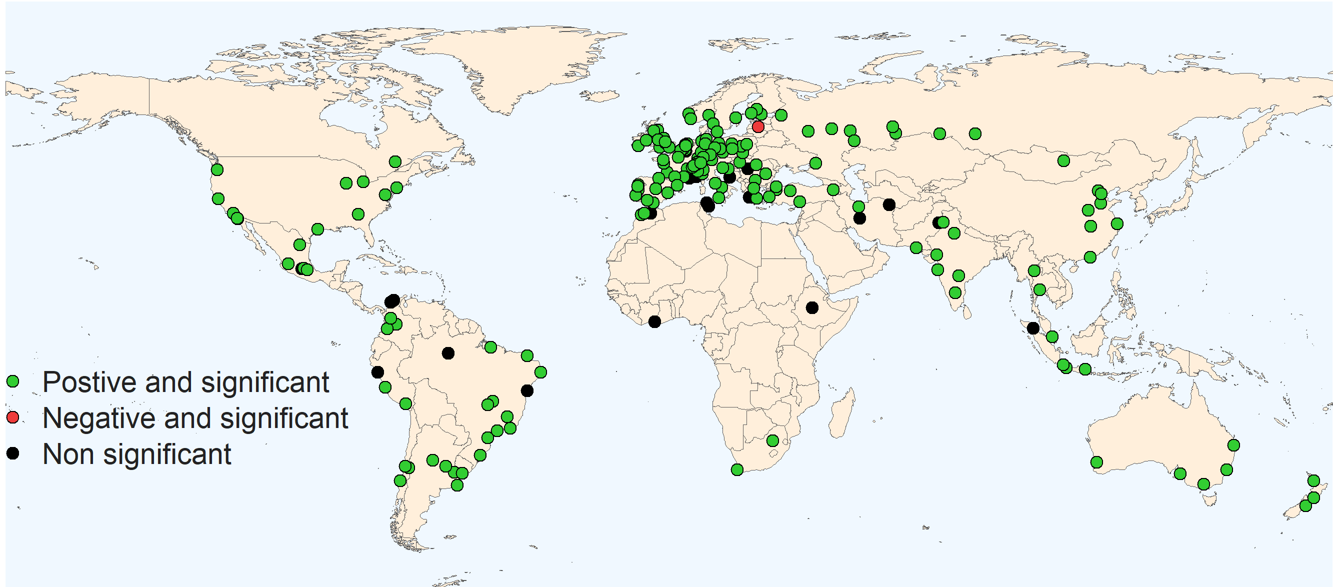
Figure 2: Map of the direction and significance of parameter $f_{c}$ (rent elasticity with respect to income net of transportation costs), estimated with 2SLS.
This parameter is positive and significant in 167 cities, negative and significant in one city, and non-significant in 23 cities.

To understand whether the relationship between accessibility and rents theorized in the SUM is verified, we also compute the R² of regression (Table 2), which can be interpreted as the percentage of the variance in rents per m² that is due to the variance in transportation costs. We find that the mean R² is 0.20 and that R² can be up to 0.66 in some cities (OLS), supporting the postulate that rents strongly depend on transportation costs to the city center but showing significant heterogeneity between cities.

	Mean	Min.	Q1	Med.	Q3	Max.	Nb. of obs.
OLS	0.20	0.00	0.06	0.18	0.31	0.66	191
2SLS	0.19	-0.17	0.04	0.16	0.30	0.66	191

Table 2: Distribution of the R² of equation 14.

Then, we analyze the value of the estimate of $f_{c}$. Figure 3 shows the distribution of these estimates. Despite a few negative or very high values (above 8), most estimates are between 0 and 6, with a median estimate of 2.71 and a mean of 3.10 (2SLS): on average for our sample of cities, when income net of transportation costs increases by 1%, rents increase by 3.1%. This can be interpreted as $\beta_{c}$ being around 1/3 in most cities, meaning that households spend around one-third of their income net of transportation costs on housing, which is consistent with the data available for the OECD countries.

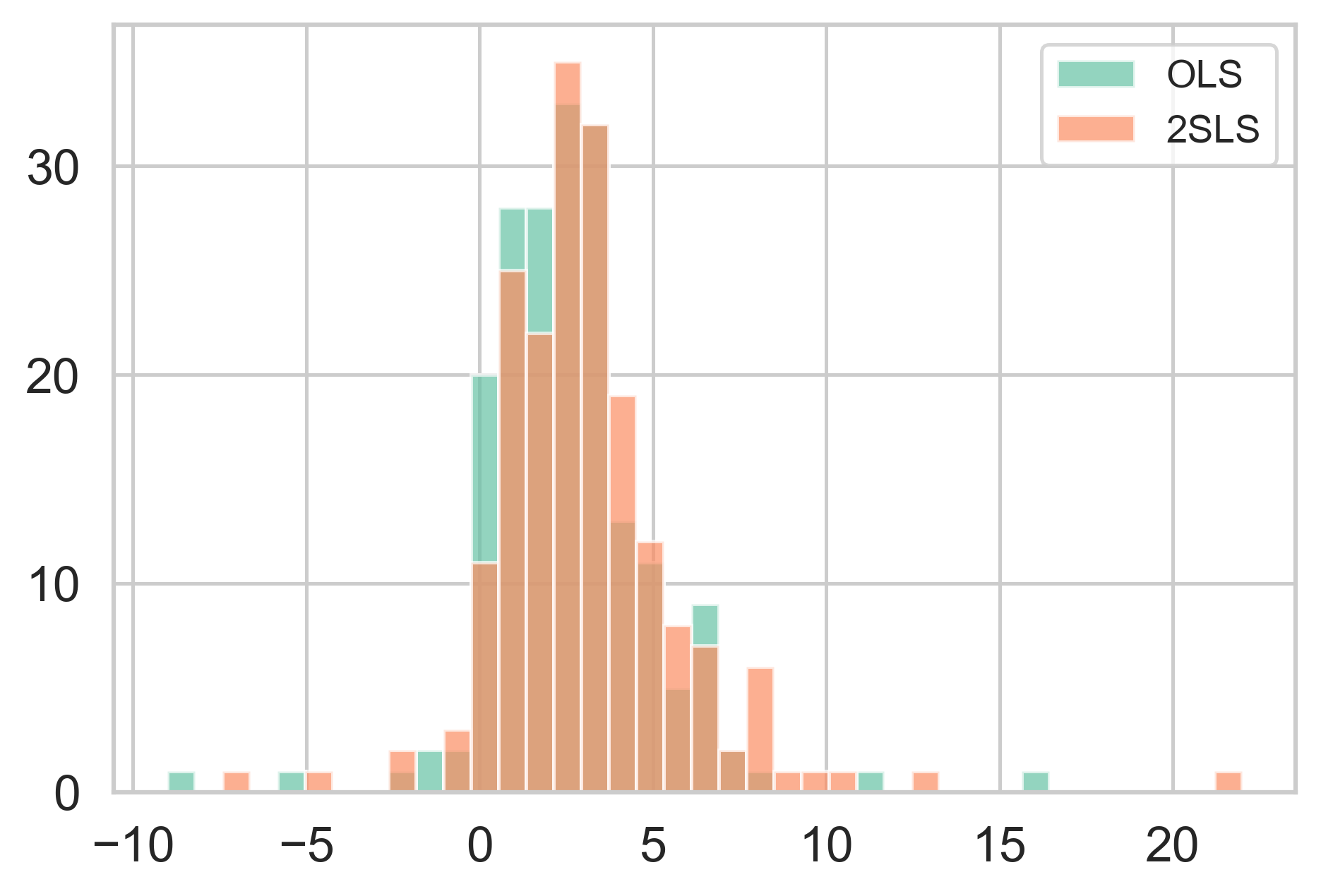
(a) Histogram - distribution of parameter f_c.

	Mean	Min.	Q1	Med.	Q3	Max.	Nb. of obs.
OLS	2.59	-8.83	1.10	2.33	3.51	16.14	191
2SLS	3.10	-6.78	1.50	2.71	4.13	21.78	191

(b) Table - distribution of parameter f_c.

Figure 3: Distribution of the estimates of parameter f_c (rent elasticity with respect to income net of transportation costs) in the 191 cities.

4.1.3 Second-step regressions

This section further examines heterogeneity in the estimates of parameter f_c. We aim to understand why rents are highly dependent on transportation costs to the city center in some cities, leading to high rent gradients, while this is not the case in others, leading to low or even inverted gradients. For that purpose, we regress our estimates of parameter f_c on a set of city characteristics based on the literature and on the intuitions derived from Figure 2 (Table 3).

In the literature, transportation costs to the city center have been found to be good predictors of rents, but their explanatory power can be mitigated by polycentrism and local amenities (see section 2.2). Therefore, in specification (1), we regress estimates of parameter f_c on monocentricity and on a dummy indicating whether the city is coastal, since the sea is in general associated with strong locational amenities that are likely to impact the real estate market. We also control for rent data quality and for population, as subcenters are more likely to emerge in more populous cities. We find that the relationship between income net of transportation costs and rents is stronger in non-coastal cities. Transportation costs to the city center are also a better predictor of rents in monocentric cities, but this coefficient is non-significant. Finally, as expected, we find a stronger relationship between rents and income net of transportation costs when our real estate data are of better quality.

In specification (2), we add three variables: the Gini index, the percentage of informal housing, and the stringency of the regulatory environment. The first two are based on our observation that the estimate of f_c seems to be non-significant in some cities with high inequalities and levels of informal housing. The third is based on Bertaud and Malpezzi (2014), who observe that the regulatory environment might affect the city’s structure. We find that the estimate of parameter f_c is lower in cities with a large percentage of informal housing. We also find higher estimates in cities for which we have good-quality data. The dummy for coastal cities is no longer significant. The categorical variable coding for stringent regulations is also non-significant at the 10% level: an explanation might be that, even in a stringently regulated city such as Moscow with a population density pattern that departs from the monocentric SUM pattern, housing prices may have initially been random, but over time consumers tend to value accessibility and housing prices tend to follow the negative density gradient, similarly to market economies (Bertaud and Malpezzi, 2014; Bertaud and Renaud, 1997).

Specification (3) includes continental fixed effects, taking Europe as the reference. In this specification, the percentage of informal housing is significant at the 1% level; we also find that the relationship between transportation costs and rents is stronger in Asian cities. Overall, in these three specifications, R² values vary between 0.073 and 0.227: we are only able to provide limited explanations of the heterogeneity in rent gradients between cities. This might be due to unobserved variables: for instance, the only amenity we account for is that provided by a coastal location, and we cannot account for other location-based or dwelling-based amenities. Another explanation might be quality of variables. The "regulatory environment" dummy, for instance, is based in some cases on the authors’ judgement and might lack accuracy. Finally, some of the explanatory variables might be correlated, such as the quality of real estate data and the percentage of informal housing.

	Dependent variable: rent gradients fc
	(1)	(2)	(3)
Coastal city	-0.700∗	-0.602	-0.395
	(0.408)	(0.408)	(0.409)
Monocentricity index	0.196	-0.318	0.567
	(0.426)	(0.479)	(0.487)
log(population)	-0.132	0.161	-0.255
	(0.183)	(0.221)	(0.236)
Market data cover	-0.000	-0.000	-0.000∗∗
	(0.000)	(0.000)	(0.000)
Spatial data cover	7.474∗∗∗	6.707∗∗	3.196
	(2.625)	(2.657)	(2.593)
Gini index		-0.045	-0.037
		(0.030)	(0.044)
Percentage of informal housing		-0.035∗	-0.091∗∗∗
		(0.021)	(0.026)
Regulatory environment		0.265	0.374
		(0.413)	(0.404)
Asia			4.065∗∗∗
			(0.919)
Africa			0.329
			(1.213)
Oceania			-1.275
			(0.994)
North America			-0.060
			(0.946)
South America			1.429
			(0.987)
Constant	4.035	2.955	6.576∗∗
	(2.868)	(3.029)	(3.213)
Observations	191	191	191
$R^{2}$	0.073	0.104	0.227
Adjusted $R^{2}$	0.048	0.065	0.170
F Statistic	2.904∗∗	2.647∗∗∗	4.002∗∗∗
Note:	∗p$<$0.1; ∗∗p$<$0.05; ∗∗∗p$<$0.01

Table 3: Second-step regression of the estimates of rent gradients f_c against city characteristics.

4.1.4 Robustness checks

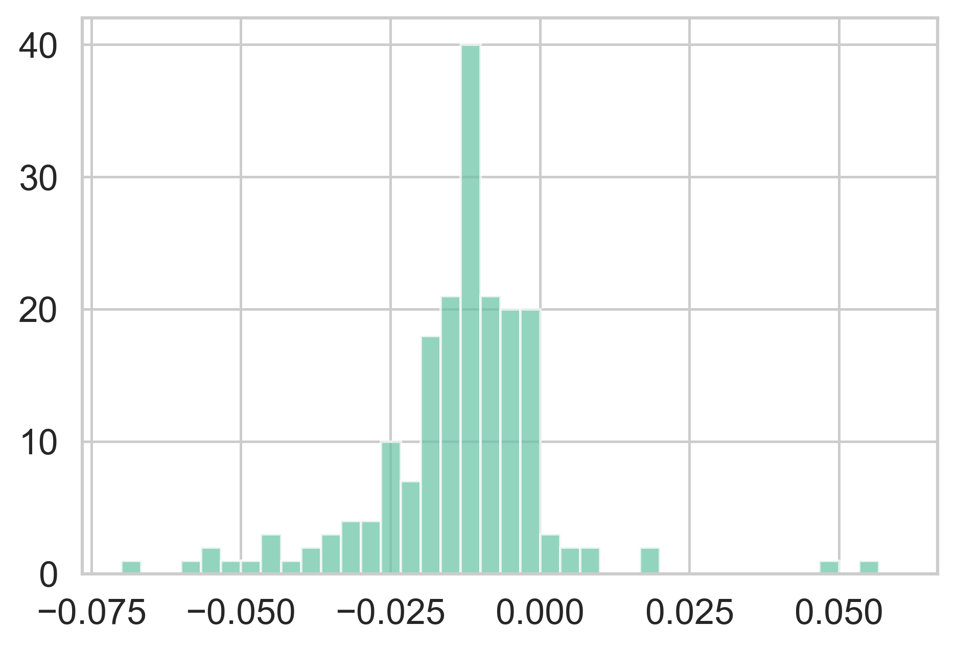
(a) Histogram - distribution of parameter f’_c.

	Mean	Min.	Q1	Med.	Q3	Max.	Nb. of obs.
OLS	-0.014	-0.070	-0.019	-0.012	-0.006	0.056	191

(b) Table - distribution of parameter f’_c.

Figure 5: Distribution of the estimates of parameter f’_c (rent gradient estimated with Robustness check 1) in the 191 cities.

We run some robustness checks for alternative specifications of equation 14. In particular, we regress the logarithm of rents per m² on the Euclidean distance from the city center, instead of considering the logarithm of the income net of transportation costs. On average, in the sample of cities, we find a gradient of -0.014, meaning that going 1km farther from the city center decreases rents per sqm by 1.4% (B, Figure 5). We also find heterogeneity in the estimates of this gradient between cities: the interquartile range is -0.019 - -0.006, and the results of the second-step regression show that this gradient is steeper in Asia and South America, and flatter in cities with a large percentage of informal housing.

We run some additional robustness checks, including regressing the logarithm of rents per m² on the logarithms of transportation costs or transportation times instead of regressing them on the logarithm of incomes nets of transportation costs. Full details and results are in B. Overall, our results are robust to alternative specifications. Depending on the robustness check performed, a rent gradient of the expected direction is found in between 157 and 167 cities. The percentage of informal housing, the data quality, and the continental fixed-effects are found to impact the value of the rent gradient in all robustness checks.

To summarize this subsection, despite the rent gradient having rarely been studied in the literature, in particular in developing countries, we found a gradient of the expected direction in most of the cities in our sample, with a mean elasticity of around 3 that can structurally be interpreted as households spending on average one-third of their income net of transportation costs on housing. However, low data quality or a high percentage of informal housing make the rent gradient flatter, so that an important direction for future research should be to adapt the monocentric SUM to such local contexts.

4.2 Density gradients

4.2.1 Empirical strategy

This subsection examines a second relationship derived from the SUM: the negative population density gradient from the city center to the periphery. We expect population density to decrease with transportation costs or increase with income net of transportation costs. Building on equation 10, we run the following regression on the sampled cities:

$$ln(n_{i,c}){\displaystyle=\,}g_{c}+h_{c}ln(Y_{c}-T_{i,c})+\text{\textrtailn}_{i,c}$$ (15)

We run this regression 192 times to individually estimate $g_{c}$ and $h_{c}$ for all the sampled cities. The error term $\text{\textrtailn}_{i,c}$ accounts for the fact that locations within cities differ in attributes other than transportation costs. We can structurally interpret parameters $h_{c}$ as $(1/\beta_{c}a_{c})-1$.

We empirically measure the income net of transportation costs as in the previous subsection and use the Euclidean distance to the city center as an instrumental variable. Population density in city c and pixel i is measured as $n_{i,c}=\frac{N_{i,c}}{L_{i,c}}$ with $N_{i,c}$ the total population in the pixel derived from the GHSL data and $L_{i,c}$ the amount of urbanizable land in the pixel derived from ESA CCI land cover data.

4.2.2 Results

We start by analyzing the sign of parameter $h_{c}$. Based on the theory, we expect this parameter to be positive: population density should decrease when transportation costs increase, or when income net of transportation costs decreases. Empirically estimating this parameter in our sample, we find that it is significantly positive at the 10% level in all the cities.

Table 4 shows the distribution of the R² of regression 15 in the sampled cities, which can be interpreted as the percentage of the variance in population densities explained by accessibility. We find a median R² of 0.17 and a maximum of 0.46, meaning that accessibility is a strong determinant of population densities in a large number of cities in our sample. These R² figures are not as high as in some existing studies (such as Bertaud and Malpezzi (2014)): an explanation is that we analyze our data at a highly disaggregated level, not grouping them by rings for instance (Duranton and Puga, 2015).

	Mean	Min.	Q1	Med.	Q3	Max.	Nb. of obs.
OLS	0.19	0.02	0.12	0.17	0.24	0.46	192
2SLS	0.15	-1.12	0.09	0.15	0.23	0.46	192

Table 4: Distribution of the R² of equation 15.

Figure 4 shows the distribution of the estimates of parameter $h_{c}$ in the sampled cities. The mean estimate is 21.17, meaning that, on average, in our sample, when income net of transportation costs decreases by 1%, population density decreases by 21.17%. However, despite being always positive, estimates are highly heterogeneous between cities. The minimum is 2.5, the maximum 58.7, and the interquartile range 13.2 - 27.5 (2SLS).

We can structurally derive the elasticity of housing production with respect to land and capital (parameters $a_{c}$ and $b_{c}$ from equation 4). From equation 10, $h_{c}=\frac{1-\beta_{c}a_{c}}{\beta_{c}a_{c}}$, and from equation 3, $f_{c}=\frac{1}{\beta_{c}}$, meaning that we can derive $a_{c}$ as $\frac{f_{c}}{1+h_{c}}$. Using the estimates of $f_{c}$ from subsection 4.1 and the estimates of $h_{c}$ from this subsection, we find that the median estimate of the elasticity of housing production with respect to land $a_{c}$ over the sample of cities is 0.13 (interquartile range of 0.08-0.21) and that the median estimate of the elasticity of housing production with respect to capital $b_{c}$ over the sample of cities is 0.87 (interquartile range of 0.79 - 0.92). Our results are in line with Epple et al. (2010), who estimate a land elasticity of 0.14, but slightly differ from Combes et al. (2021), who estimate a capital elasticity of 0.65 for France.

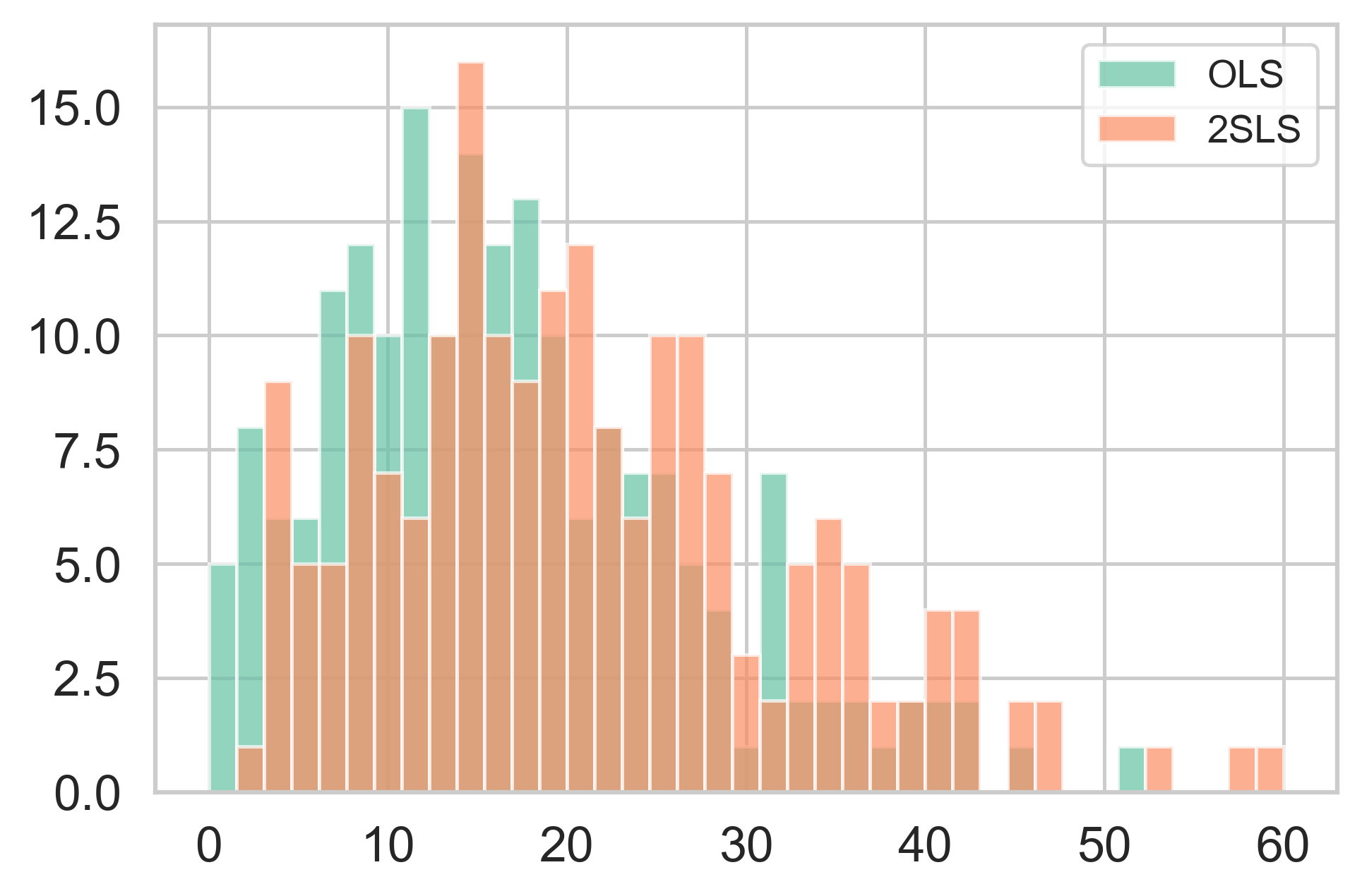
(a) Histogram - distribution of parameter h_c.

	Mean	Min.	Q1	Med.	Q3	Max.	Nb. of obs.
OLS	16.70	0.84	9.28	15.19	22.33	50.94	192
2SLS	21.17	2.50	13.19	19.48	27.46	58.68	192

(b) Table - distribution of parameter h_c.

Figure 4: Distribution of the estimates of parameter h_c (elasticity of population density with respect to the income net of transportation costs) in the 192 cities.

4.2.3 Second-step regressions

This section further investigates the heterogeneity in density gradients by regressing our estimates of h_c against city characteristics (Table 5).

Specification (1) is based on the density gradient literature, which suggests that polycentrism leads to flatter density gradients. Some studies show that larger populations lead to flatter gradients, an explanation being that employment subcenters are more likely to emerge in larger urban areas (see subsection 2.2.1). Incomes and transportation costs have also been found to play a role in explaining density gradients (see subsection 2.2.1). However, they are already accounted for in our first step empirical regressions (equation 15), and therefore we do not need to include them in this second-step regression.

Empirically testing these hypotheses, we find that larger (in terms of population) and more polycentric urban areas tend to have flatter density gradients. The R² of this first specification is 0.38, meaning that population and polycentricity explain a large percentage of the variance in density gradients across urban areas. Since, here, population is included in the second-step regression as an indicator of polycentricity, it may be surprising that population and monocentricity are both significant. We attribute this to the quality of our monocentricity index: it indicates whether the historical, geographical, transportation, administrative, and business centers are all located in the same place, but it does not indicate whether the city has a large number of subcenters, which is proxied by the city’s population. Thus, the total population and the monocentricity index correspond to two different definitions of monocentricity.

In specification (2), we add four explanatory variables: the level of inequalities, the percentage of informal housing, and two categorical variables indicating whether the city is coastal and whether there is a stringent regulatory environment. The first two variables are based on our observation that rent gradients seem to be flattened in cities with a large percentage of informal housing or inequalities (Figure 2). The two categorical variables are based on Bertaud and Malpezzi (2014), who find that complex geographies or stringent regulatory environments flatten the density gradient.We find that a large percentage of informal housing and high inequality levels tend to flatten the population density gradient, the two variables being significant at the 1% level. Monocentricity and population remain significant as well.

Specification (3) adds continent fixed effects, taking Europe as the reference. Population, monocentricity, and informal housing remain significantly different from 0 at the 1%, 1%, and 5% levels respectively: cities with larger populations, more subcenters, and more informal housing tend to have flatter density gradients. Surprisingly, the dummy for stringent regulatory environments is positive and significant at the 10% level, meaning that cities with strong regulations tend to have steeper density gradients, which contrasts with Bertaud and Malpezzi (2014). However, as Bertaud (2004) has observed, some cities subject to stringent regulations developed before the implementation of the latter, and have kept an urban form that is to some extent similar to market-oriented cities. For instance, Central and Eastern European cities, such as Cracow, were stringently regulated during the socialist era, but these cities had a large historical center established many centuries before socialism so that they have remained largely monocentric. Finally, African and Oceanian cities tend to have flatter density gradients.

	Dependent variable: population density gradients hc
	(1)	(2)	(3)
log(population)	-5.895∗∗∗	-4.192∗∗∗	-5.428∗∗∗
	(0.626)	(0.690)	(0.856)
Monocentricity index	6.525∗∗∗	3.148∗∗	4.346∗∗∗
	(1.314)	(1.463)	(1.591)
Gini index		-0.263∗∗∗	-0.104
		(0.087)	(0.147)
Percentage of informal housing		-0.218∗∗∗	-0.176∗∗
		(0.053)	(0.070)
Coastal city		0.386	1.583
		(1.362)	(1.508)
Regulatory environment		2.512	3.119∗
		(1.584)	(1.749)
Asia			2.602
			(3.939)
Africa			-8.157∗∗∗
			(2.968)
Oceania			-9.958∗∗∗
			(2.442)
North America			2.598
			(3.429)
South America			-3.264
			(3.801)
Constant	92.486∗∗∗	86.716∗∗∗	95.918∗∗∗
	(10.650)	(11.113)	(12.958)
Observations	192	192	192
$R^{2}$	0.375	0.448	0.508
Adjusted $R^{2}$	0.368	0.430	0.478
F Statistic	70.21∗∗∗	40.15∗∗∗	29.49∗∗∗
Note:	∗p$<$0.1; ∗∗p$<$0.05; ∗∗∗p$<$0.01

Table 5: Second-step regression of population density gradient estimates h_c against city characteristics.

4.2.4 Robustness checks

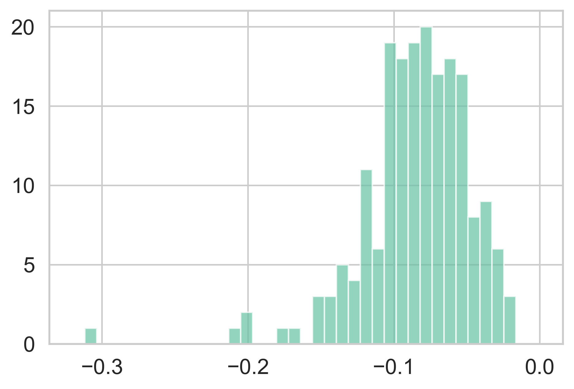
(a) Histogram - distribution of parameter h’_c.

	Mean	Min.	Q1	Med.	Q3	Max.	Nb. of obs.
OLS	-0.085	-0.309	-0.102	-0.081	-0.060	-0.017	192

(b) Table - distribution of parameter h’_c.

Figure 6: Distribution of the estimates of parameter h’_c (density gradient estimated with Robustness check 1) in the 192 cities.

We run some robustness checks for alternative specifications of equation 15. In particular, we regress the logarithm of population density on the Euclidean distance from the city center, instead of considering the logarithm of the income net of transportation costs. On average, in the sample of cities, we find a gradient of -0.085, meaning that going 1km farther from the city center decreases population density by 8.5% (B, Figure 6). We find some heterogeneity in the estimates of this gradient between cities: the interquartile range is -0.102 - -0.060, and results of the second-step regression show that this gradient is flatter in North America, Oceania, and when the city is larger in terms of population, and steeper when the city is coastal or has a large percentage of informal housing.

We run some additional robustness checks, including regressing the logarithm of population densities on the logarithm of transportation costs or transportation times instead of regressing them on the logarithm of incomes nets of transportation costs. Full details and results are in B. Overall, our results are robust to alternative specifications. A density gradient of the expected direction is found in all of the cities and with all robustness checks. The population of the city, its monocentricity, and continent-fixed effects are found to impact the value of the density gradient in most of the robustness checks. The percentage of informal housing has an impact on density gradients in some of the robustness checks performed.

To summarize this subsection, we find that the expected negative population density gradient is observed in all of the cities in our sample. In addition, in line with the literature, we found flatter density gradients in larger, and more polycentric, cities. A direction for future research should be incorporating informality into urban models, as we also observed flatter density gradients in cities with large percentages of informal housing.

4.3 Urban area

This subsection examines whether the size of urban areas increases with population and income and decreases with farmland rents and transportation costs, as suggested by the SUM (equation 13).

In the first specification (“all cities”) of Table 6, we regress urbanized areas on a range of city characteristics derived from the theory (subsection 2.1), including populations, incomes, and farmland rents. We add two commuting cost variables: fuel price and "commuting speed", which is the density-weighted average speed when traveling to the city center during the evening rush hour using the fastest transportation mode (car or public transport). We also include the monocentricity index, as many studies argue that polycentricity impacts the size of urban areas. Spivey (2008) finds that more sub-centers are associated with a smaller land area in the United States, which she interprets as the fact that sub-centers are more likely to develop in dense areas or that increased density associated with sub-centers mitigates sprawl. Paulsen (2012) confirms this result. In contrast, Burchfield et al. (2006) find that decentralized employment increases sprawl in the US. Schmidt et al. (2020) find non-significant estimates of the impact of polycentricity on the size of urban areas in Germany.

We find an R² of 0.86, meaning that city characteristics explain a large percentage of the variance in the size of urbanized areas among the sampled cities. In addition, all the coefficients of the explanatory variables are significant and of the expected sign, except for fuel price. For instance, a 1% increase in population leads to a 0.86% increase in the urban area, in line with Spivey (2008), which finds an elasticity of 0.91, and slightly higher than Paulsen (2012), which finds elasticities of between 0.56 and 0.64. We also find that a 1% increase in incomes leads to a 0.40% increase in the urban area. An increase in farmland rents tends to decrease urban areas, and an increase in commuting speed, corresponding to a decrease in the opportunity cost of transportation, increases urban areas. The non-significant estimate for fuel price might be caused by cities’ inertia when compared to the relative volatility of fuel prices. Finally, for monocentricity, we find a positive coefficient significant at the 10% level, in line with Spivey (2008).

	Dependent variable: log(urbanized area)
	All cities	High income	Upper-middle income
			to low income
log(population)	0.856∗∗∗	0.913∗∗∗	0.778∗∗∗
	(0.040)	(0.067)	(0.047)
log(income)	0.397∗∗∗	0.277∗∗	0.436∗∗∗
	(0.038)	(0.125)	(0.055)
log(farmland rents)	-0.220∗∗∗	-0.311∗∗∗	-0.076
	(0.043)	(0.056)	(0.047)
log(fuel price)	-0.061	0.125	-0.153
	(0.101)	(0.213)	(0.136)
log(commuting speed)	0.466∗∗∗	0.434∗∗	0.563∗∗∗
	(0.100)	(0.168)	(0.132)
Monocentricity index	0.146∗	0.101	0.199∗∗
	(0.082)	(0.172)	(0.085)
Constant	-12.876∗∗∗	-12.413∗∗∗	-12.070∗∗∗
	(0.624)	(0.998)	(0.847)
Observations	192	108	84
$R^{2}$	0.858	0.866	0.878
Adjusted $R^{2}$	0.853	0.858	0.869
F Statistic	225.7∗∗∗	184.9∗∗∗	96.78∗∗∗
Note:	∗p$<$0.1; ∗∗p$<$0.05; ∗∗∗p$<$0.01

Table 6: Regression of urbanized areas against city characteristics.

To further investigate the heterogeneity in the determinants of urbanized areas between cities, we slice the result by income levels. “High income” cities are those located in high-income countries, according to the World Bank classification. “Upper-middle income to low income” corresponds to the cities located in upper-middle, lower-middle, or low income countries according to the World Bank classification. In our sample, all North American and Oceanian cities are classified as high-income, as well as 2 Asian cities (Hong Kong and Singapore), 4 South American cities (in Uruguay and Chile), and most European cities (83/97). The remaining cities are all African cities, most Asian cities (30/32), and most South American cities (30/34). This classification allows us to split our sample into two groups each containing a similar number of cities, with each group broadly corresponding to three continents. Unfortunately, we cannot slice the results by continent due to data limitations: we do not have enough cities for some continents (we only have 8 cities for Oceania and 10 cities for Africa) or enough heterogeneity within continents (the fact that all of the North American cities of the sample are located in the USA is problematic because we only have data at the country level for some explanatory variables).

We run a Chow test to check whether we need separate models for these two groups of cities. The test is significant at the 5% level, meaning that the differences in estimated coefficients across the two sub-samples are not the result of sampling error.

We find that an increase in population has a larger impact on the size of urbanized areas in high-income cities than in other cities, whereas income has a larger impact on the size of urbanized areas in middle and low-income cities. The latter result is in line with the studies that find that income growth is a large driver of urban sprawl in developing countries (Deng et al., 2008; Ke et al., 2009). It is also in line with Schmidt et al. (2020): they find that income has a low impact on urban sprawl in Germany, which they explain by the growth management policies that eliminate the impact of income in Germany. Farmland rents have a large negative impact on urban sprawl in high-income countries, in line with the findings of Oueslati et al. (2015): they found a high coefficient for farmland rents, which, according to the authors, reflects the fact that in Europe, agriculture on the urban fringe is often highly intensive, offering relatively high yields and profits. Commuting speed has a smaller impact on high-income countries. Finally, monocentricity is non-significant in high-income countries, whereas it is significant for middle-income and low-income countries.

5 Conclusion

Exploiting a new spatially-explicit dataset on population densities, land cover, but also real estate and transportation costs, we are able to empirically assess the main relationships derived from the SUM in a large and diverse sample of cities. In particular, we can assess the SUM’s predictions in terms of internal city structures, evaluating density and rent gradients in 192 global cities.

Although the SUM is an old, simple model, we show that its main predictions are verified for our sample of cities. We find the expected declining rent gradient from city centers to suburbs in 167 out of 192 cities and the expected declining density gradient from city centers to suburbs in all the sampled cities. In addition, we find that the total urbanized area of a city tends to increase with population and income and decrease with farmland rents and transportation costs, as expected from the theory.

Our dataset also allows us to investigate heterogeneity in the internal structures of cities. Large or polycentric cities are more likely to have flat density gradients, as are cities with a higher percentage of informal housing. Cities are more likely to have flat or inverted rent gradients if they have a large percentage of informal housing or if the quality of our rent data is lower. Overall, urban sprawl in high-income cities is largely driven by population and farmland rents, whereas income plays a key role in developing countries.

This result implies that the SUM does not perfectly fit all cities. Coastal amenities, polycentricity, and informal housing can lead to flatter, and sometimes inverted, rents and density gradients, so that modelling cities more accurately requires more complex models that account for these dimensions, in particular beyond the SUM’s traditional application area (North America, Europe).

A first limitation of this study is that it only assesses the simplest version of the SUM. Indeed, data were missing that would have enabled systematic study of more advanced urban models. Gathering data on employment subcenters and transportation costs to these employment centers is, for instance, outside the scope of this study. However, the development of new big data approaches will allow this gap to be filled in future research (Barzin et al., 2022).

Another limitation is that the SUM is mostly a static model, whereas there is inertia in cities’ development. Densities and built environment are changing slowly (as are transport times, to some extent), whereas rents and land prices can change quickly. Obtaining panel data on cities would be necessary in order to study changes in city structures over time.

References

Annex A Land cover classification

ESA CCI land cover category	Reclassification
10 Cropland, rainfed	Urbanizable
11 Herbaceous cover	Urbanizable
12 Tree or shrub cover	Urbanizable
20 Cropland, irrigated or post-flooding	Urbanizable
30 Mosaic cropland (>50%) / natural vegetation (<50%)	Urbanizable
40 Mosaic natural vegetation (>50%) / cropland (<50%)	Urbanizable
50 Tree cover, broadleaved, evergreen, closed to open (>15%)	Urbanizable
60 Tree cover, broadleaved, deciduous, closed to open (>15%)	Urbanizable
61 Tree cover, broadleaved, deciduous, closed (>40%)	Urbanizable
62 Tree cover, broadleaved, deciduous, open (15-40%)	Urbanizable
70 Tree cover, needleleaved, evergreen, closed to open (>15%)	Urbanizable
71 Tree cover, needleleaved, evergreen, closed (>40%)	Urbanizable
72 Tree cover, needleleaved, evergreen, open (15-40%)	Urbanizable
80 Tree cover, needleleaved, deciduous, closed to open (>15%)	Urbanizable
81 Tree cover, needleleaved, deciduous, closed (>40%)	Urbanizable
82 Tree cover, needleleaved, deciduous, open (15-40%)	Urbanizable
90 Tree cover, mixed leaf type (broadleaved and needleleaved)	Urbanizable
100 Mosaic tree and shrub (>50%) / herbaceous cover (<50%)	Urbanizable
110 Mosaic herbaceous cover (>50%) / tree and shrub (<50%)	Urbanizable
120 Shrubland	Urbanizable
121 Evergreen shrubland	Urbanizable
122 Deciduous shrubland	Urbanizable
130 Grassland	Urbanizable
140 Lichens and mosses	Urbanizable
150 Sparse vegetation (tree, shrub, herbaceous cover) (<15%)	Urbanizable
160 Tree cover, flooded, fresh or brackish water	Non urbanizable
170 Tree cover, flooded, saline water	Non urbanizable
180 Shrub or herbaceous cover, flooded, fresh/saline/brakish water	Non urbanizable
190 Urban areas	Urbanizable
200 Bare areas	Urbanizable
201 Consolidated bare areas	Urbanizable
202 Unconsolidated bare areas	Urbanizable
210 Water bodies	Non urbanizable
220 Permanent snow and ice	Non urbanizable

Table 7: Reclassification of the ESA CCI land cover categories into "urbanizable" and "non urbanizable"

Annex B Robustness checks

B.1 Description of the robustness checks

We run five robustness checks, detailed below, for subsections 4.1 and 4.2. In robustness check 1, our variable of interest is the Euclidean distance to the city center $d_{i,c}$ instead of the income net of transportation costs $Y_{c}-T_{i,c}$. Our theoretical model is similar to subsection 2.1, except that households seek to maximize the following utilities:

$$max\hskip 8.53581ptU(z_{i,c},\,q_{i,c},d_{i,c})=z_{i,c}^{\alpha_{c}}\,q_{i,c}^{\beta_{c}}l(d_{i,c})\quad s.t.\hskip 8.53581ptz_{i,c}+q_{i,c}R_{i,c}\leq Y_{c}$$ (16)

with $l$ an amenity that depends on the Euclidean distance to the city center $d_{i,c}$. From equation 16, we find that:

$$\begin{array}[]{l}q_{i,c}=\beta_{c}Y_{c}/R_{i,c}\\ z_{i,c}=\alpha_{c}Y_{c}\end{array}$$ (17)

Using the spatial equilibrium condition and writing $u_{c}$ the utility at equilibrium:

$$R_{i,c}=R_{0,c}\,l(d_{i,c})^{1/\beta_{C}}\hskip 28.45274pt\text{with}\hskip 28.45274ptR_{0,c}=(\frac{\alpha_{c}^{\alpha_{c}}\,\beta_{c}^{\beta_{c}}\,Y_{c}}{u_{c}})^{1/\beta_{c}}$$ (18)

The housing production function remains unchanged from section 2.1:

$$H(K_{i,c},\,L_{i,c})=A_{c}\,L_{i,c}^{a_{c}}\,K_{i,c}^{b_{c}}$$ (19)

As in subsection 2.1, from the profit maximization of private developers, we can derive the total population per pixel $N_{i,c}$:

$$N_{i,c}=H_{i,c}/q_{i,c}=A_{c}^{1/a_{c}}(b_{c}R_{i,c}/\rho)^{b_{c}/a_{c}}L_{i,c}/q_{i,c}$$ (20)

Replacing $q_{i,c}$ and $R_{i,c}$ by their expressions in equations 17 and 18, the population density par pixel $n_{i,c}=N_{i,c}/L_{i,c}$ can be expressed as:

$$n_{i,c}=A_{c}^{1/a_{c}}(\frac{b_{c}}{\rho})^{b_{c}/a_{c}}(\frac{\alpha_{c}^{\alpha_{c}}}{u})^{1/(\beta_{c}a_{c})}\beta_{c}^{b_{c}/a_{c}}Y_{c}^{(1-a_{c}\beta_{c})/a_{c}\beta_{c}}l(d_{i,c})^{1/a_{c}\beta_{c}}$$ (21)

Our empirical strategy is then as follows: assuming that $l(d_{i,c})=\kappa e^{-\theta d_{i,c}}$and building on equations 18 and 21, we run the following regressions on the cities in the database:

$$ln(R_{i,c})=e^{\prime}_{c}+f^{\prime}_{c}d_{i,c}+\varepsilon^{\prime}_{i,c}$$ (22)

$$ln(n_{i,c})=g^{\prime}_{c}+h^{\prime}_{c}d_{i,c}+\eta^{\prime}_{i,c}$$ (23)

$e^{\prime}_{c}$ and $g^{\prime}_{c}$ are constants, $\varepsilon^{\prime}_{c}$ and $\eta^{\prime}_{c}$ are error terms, and $f^{\prime}_{c}$ and $h^{\prime}_{c}$ can be structurally interpreted as $-\theta/\beta_{c}$ and $\frac{-\theta}{a_{c}\beta_{c}}$ respectively.

In addition to robustness check 1, we run four additional robustness checks:

• Robustness check 2: We regress the logarithm of population densities and rents on the logarithm of transportation costs, instead of the logarithm of income net of transportation costs. We substitute $T_{i,c}$ for $Y_{c}-T_{i,c}$ in equations 14 and 15.

• Robustness check 3: We regress the logarithm of population densities and rents on the logarithm of transportation times (taking the minimum of the transportation time by driving and public transport). We substitute the minimum of the transportation time by driving and public transport $t_{i,c}=min(t_{i,c}^{driving},t_{i,c}^{publictransport})$ for $Y_{c}-T_{i,c}$ in equations 14 and 15.

• Robustness check 4: We regress the logarithm of population densities and rents on the logarithm of incomes net of transportation costs, but omitting the monetary cost of public transport as data are not consistently available for all cities.

• Robustness check 5: We regress the logarithm of population densities and rents on the logarithm of incomes net of transportation costs (equation 14). However, instead of taking the average rent per grid cell, rent data are aggregated by regressing rents on dwelling sizes in each grid cell (this robustness check is relevant for results regarding rent gradients, but does not affect the results regarding density gradients).

B.2 Robustness checks - Rent gradients

With our main specification (subsection 4.1), we find rent gradients of the expected direction in 160 cities with OLS and 167 with 2SLS (Figure 2). We investigate whether this result holds under the five robustness checks (Table 8).

		Expected	Opposite	Non-significant
		direction	direction	(10% level)
Main specification	OLS	160	29	2
Main specification	2SLS	167	23	1
Robustness check 1	OLS	160	29	2
Robustness check 2	OLS	163	27	1
Robustness check 2	2SLS	167	23	1
Robustness check 3	OLS	162	28	1
Robustness check 3	2SLS	167	23	1
Robustness check 4	OLS	159	30	2
Robustness check 4	2SLS	167	23	1
Robustness check 5	OLS	157	32	2
Robustness check 5	2SLS	161	29	1

Table 8: Robustness checks – direction of rent gradients.

With our main specification (subsection 4.1), we find that the median R² of regression 14 is 0.18 with OLS and 0.16 with 2SLS (Table 2). We investigate whether this result holds under the five robustness checks (Table 9).

		Mean	Min.	Q1	Med.	Q3	Max.
Main specification	OLS	0.20	0.00	0.06	0.18	0.31	0.66
Main specification	2SLS	0.19	-0.17	0.04	0.16	0.30	0.66
Robustness check 1	OLS	0.20	0.00	0.06	0.17	0.31	0.61
Robustness check 2	OLS	0.20	0.00	0.07	0.18	0.32	0.64
Robustness check 2	2SLS	0.20	-0.00	0.07	0.17	0.31	0.64
Robustness check 3	OLS	0.19	0.00	0.06	0.17	0.29	0.63
Robustness check 3	2SLS	0.19	-0.02	0.06	0.16	0.27	0.62
Robustness check 4	OLS	0.19	0.00	0.06	0.17	0.30	0.59
Robustness check 4	2SLS	0.17	-0.17	0.04	0.16	0.29	0.56
Robustness check 5	OLS	0.18	0.00	0.04	0.15	0.28	0.66
Robustness check 5	2SLS	0.17	-0.13	0.03	0.14	0.27	0.66

Table 9: Robustness checks - R² of equation 14.

Then, we display the distribution of the rent gradients estimated in Robustness check 1. On average, moving 1km farther from the city center reduces rents per m² by 1.4%.

With our main specification (subsection 4.1), we find that the market data cover, the percentage of informal housing, and the dummy indicating whether the city is located in Asia explain the estimated rent gradients (Table 3). We investigate whether this result holds under the five robustness checks (Table 10).

	Dependent variable: rents gradients
	Main	Robustness	Robustness	Robustness	Robustness	Robustness
	specification	check 1	check 2	check 3	check 4	check 5
Coastal city	-0.395	0.003	0.016	0.001	-0.352	-0.530
	(0.409)	(0.002)	(0.028)	(0.033)	(0.414)	(0.432)
Monocentricity index	0.567	-0.002	0.004	0.007	0.580	0.663
	(0.487)	(0.003)	(0.035)	(0.040)	(0.493)	(0.514)
log(population)	-0.255	0.001	-0.091***	-0.092***	-0.280	-0.207
	(0.236)	(0.001)	(0.017)	(0.019)	(0.239)	(0.250)
log(income)		0.001	-0.042	-0.049
		(0.002)	(0.031)	(0.036)
Market data cover	-0.000**	0.000***	0.000***	0.000***	-0.000**	-0.000**
	(0.000)	(0.000)	(0.000)	(0.000)	(0.000)	(0.000)
Spatial data cover	3.196	0.010	0.128	0.134	3.545	3.273
	(2.593)	(0.015)	(0.204)	(0.234)	(2.622)	(2.737)
Gini index	-0.037	0.000	0.004	0.004	-0.038	-0.013
	(0.044)	(0.000)	(0.003)	(0.004)	(0.045)	(0.047)
Informal housing	-0.091***	0.000***	0.006***	0.007***	-0.092***	-0.084***
	(0.026)	(0.000)	(0.002)	(0.002)	(0.026)	(0.027)
Regulatory environment	0.374	-0.003	-0.034	-0.044	0.394	-0.064
	(0.404)	(0.002)	(0.029)	(0.034)	(0.408)	(0.426)
Asia	4.065***	-0.022***	-0.173**	-0.024***	4.041***	3.999***
	(0.919)	(0.005)	(0.069)	(0.079)	(0.930)	(0.970)
Africa	0.329	-0.002	0.025	-0.012	0.203	0.454
	(1.213)	(0.007)	(0.093)	(0.107)	(1.227)	(1.280)
Oceania	-1.275	0.004	0.015	0.040	-1.309	-0.950
	(0.994)	(0.005)	(0.070)	(0.080)	(1.006)	(1.049)
North America	-0.060	0.002	0.131*	0.140*	-0.210	-0.096
	(0.946)	(0.005)	(0.071)	(0.078)	(0.998)	(0.999)
South America	1.429	-0.014***	-0.091	-0.117	1.346	1.135
	(0.987)	(0.005)	(0.071)	(0.081)	(0.998)	(1.042)
Constant	6.576**	-0.052*	1.292***	1.352***	7.030**	4.482
	(3.213)	(0.030)	(0.407)	(0.467)	(3.249)	(3.391)
Observations	191	191	191	191	191	191
R2	0.227	0.266	0.319	0.297	0.234	0.194
Adjusted R2	0.170	0.208	0.264	0.241	0.178	0.135
F Statistic	4.002***	5.559***	5.880***	5.301***	4.159***	3.281***
Note:	∗p$<$0.1; ∗∗p$<$0.05; ∗∗∗p$<$0.01

Table 10: Second-step regression of the estimates of rent gradients against city characteristics.

B.3 Robustness checks - Density gradients

With our main specification (subsection 4.2), we find density gradients of the expected direction in 192 cities with OLS and 192 with 2SLS. We investigate whether this result holds under the four robustness checks (Table 11).

		Expected	Opposite	Non-significant
		direction	direction	(10% level)
Main specification	OLS	192	0	0
Main specification	2SLS	192	0	0
Robustness check 1	OLS	192	0	0
Robustness check 2	OLS	192	0	0
Robustness check 2	2SLS	192	0	0
Robustness check 3	OLS	192	0	0
Robustness check 3	2SLS	192	0	0
Robustness check 4	OLS	192	0	0
Robustness check 4	2SLS	192	0	0

Table 11: Robustness checks – direction of the density gradients.

With our main specification (subsection 4.2), we find that the median R² of regression 15 is 0.17 with OLS and 0.15 with 2SLS (Table 4). We investigate whether this result holds under the four robustness checks (Table 12).

		Mean	Min.	Q1	Med.	Q3	Max.
Main specification	OLS	0.19	0.02	0.12	0.17	0.24	0.46
Main specification	2SLS	0.15	-1.12	0.09	0.15	0.23	0.46
Robustness check 1	OLS	0.18	0.03	0.12	0.17	0.24	0.56
Robustness check 2	OLS	0.23	0.05	0.16	0.22	0.29	0.61
Robustness check 2	2SLS	0.23	0.04	0.16	0.22	0.29	0.61
Robustness check 3	OLS	0.21	0.03	0.15	0.20	0.26	0.54
Robustness check 3	2SLS	0.20	-0.19	0.14	0.19	0.25	0.53
Robustness check 4	OLS	0.19	0.02	0.12	0.18	0.24	0.46
Robustness check 4	2SLS	0.15	-1.12	0.08	0.15	0.23	0.46

Table 12: Robustness checks - R² of equation 15.

We then display the distribution of the density gradients estimated in Robustness check 1. On average, moving 1km farther from the city center reduces poplation density by 8.5%.

With our main specification (subsection 4.2), we find that the population, the monocentricity index, the percentage of informal housing, the regulatory environment, and the dummies indicating whether the city is located in Africa and Oceania explain the estimated rent gradients (Table 5). We investigate whether this result holds under the four robustness checks (Table 13).

	Dependent variable: density gradients
	Main	Robustness	Robustness	Robustness	Robustness
	specification	check 1	check 2	check 3	check 4
log(population)	-5.428***	0.018***	-0.155**	-0.159*	-5.735***
	(0.856)	(0.003)	(0.075)	(0.091)	(0.856)
log(income)		-0.001	0.158	0.392***
		(0.005)	(0.110)	(0.138)
Monocentricity index	4.346***	-0.007	-0.316**	-0.393**	4.843***
	(1.591)	(0.007)	(0.128)	(0.178)	(1.611)
Gini index	-0.104	0.001	0.004	0.005	-0.107
	(0.147)	(0.001)	(0.011)	(0.015)	(0.146)
Percentage of informal housing	-0.176**	-0.000	0.004	0.015	-0.172**
	(0.070)	(0.000)	(0.008)	(0.011)	(0.070)
Coastal city	1.583	-0.012**	-0.133	-0.225	1.553
	(1.508)	(0.006)	(0.116)	(0.152)	(1.508)
Regulatory environment	3.119*	-0.016***	-0.141	-0.147	2.868
	(1.749)	(0.005)	(0.111)	(0.153)	(1.741)
Asia	2.602	-0.015	0.932***	1.015***	2.963
	(3.939)	(0.014)	(0.270)	(0.377)	(3.963)
Africa	-8.157***	-0.002	1.067***	1.094**	-8.148***
	(2.968)	(0.014)	(0.280)	(0.452)	(3.953)
Oceania	-9.958***	0.034***	0.059	0.138	-10.992***
	(2.442)	(0.008)	(0.324)	(0.397)	(2.283)
North America	2.598	0.022***	0.379	0.627**	2.682
	(3.429)	(0.010)	(0.238)	(0.296)	(3.423)
South America	-3.264	0.022*	0.228	-0.038	-3.503
	(3.801)	(0.016)	(0.264)	(0.402)	(3.814)
Constant	95.918***	-0.329***	-1.772	-4.628**	99.449***
	(12.958)	(0.076)	(1.677)	(2.026)	(13.071)
Observations	192	192	192	192	192
R2	0.508	0.319	0.213	0.184	0.525
Adjusted R2	0.478	0.273	0.161	0.129	0.496
F Statistic	29.49***	10.44***	4.990***	4.212***	29.85***
Note:	∗p$<$0.1; ∗∗p$<$0.05; ∗∗∗p$<$0.01

Table 13: Second-step regression of the estimates of density gradients against city characteristics.

Annex C Regulatory environmnent

When the categorical variable coding for the regulatory environment is different from 0 based on the authors’ judgements, an explanation is provided as a footnote.

City	Country	Regulatory env.	Source
Abidjan	Côte d’Ivoire	1	Bertaud and Malpezzi (2014)
Adana	Turkey	0	Authors’ judgement
Addis_Ababa	Ethiopia	0	Authors’ judgement
Adelaide	Australia	1	Authors’ judgement
Ahmedabad	India	1	Bertaud and Malpezzi (2014)
Amsterdam	Netherlands	0	Authors’ judgement
Ankara	Turkey	0	Authors’ judgement
Antwerp	Belgium	0	Authors’ judgement
Arequipa	Peru	0	Authors’ judgement
Athens	Greece	0	Authors’ judgement
Atlanta	United States of America	0	Bertaud and Malpezzi (2014)
Auckland	New Zealand	0	Authors’ judgement
Bandung	Indonesia	0	Authors’ judgement
Bangalore	India	1	Bertaud and Malpezzi (2014)
Bangkok	Thailand	0	Bertaud and Malpezzi (2014)
Barcelona	Spain	0	Bertaud and Malpezzi (2014)
Barranquilla	Colombia	0	Authors’ judgement
Basel	Switzerland	0	Authors’ judgement
Beijing	China	0	Bertaud and Malpezzi (2014)
Belem	Brazil	0	Authors’ judgement
Belo_Horizonte	Brazil	1	Authors’ judgement
Bergen	Norway	0	Authors’ judgement
Berlin	Germany	1	Bertaud and Malpezzi (2014)
Bern	Switzerland	0	Authors’ judgement
Bilbao	Spain	0	Authors’ judgement
Birmingham	United Kingdom	0	Authors’ judgement
Bogota	Colombia	0	Authors’ judgement
Bordeaux	France	0	Authors’ judgement
Braga	Portugal	0	Authors’ judgement
Brasilia	Brazil	2	Bertaud and Malpezzi (2014)
Bremen	Germany	0	Authors’ judgement
Brisbane	Australia	0	Authors’ judgement
Bristol	United Kingdom	0	Authors’ judgement
Brussels	Belgium	0	Authors’ judgement
Bucharest	Romania	0	Authors’ judgement
Budapest	Hungary	1	Bertaud and Malpezzi (2014)
Buenos_Aires	Argentina	0	Bertaud and Malpezzi (2014)
Bursa	Turkey	0	Authors’ judgement
Cali	Colombia	0	Authors’ judgement
Cape_Town	South Africa	2	Bertaud and Malpezzi (2014)
Cartagena	Colombia	0	Authors’ judgement
Casablanca	Morocco	0	Authors’ judgement
Charleroi	Belgium	0	Authors’ judgement
Chelyabinsk	Russian Federation	0	Authors’ judgement
Chiang_Mai	Thailand	0	Authors’ judgement
Chicago	United States of America	0	Bertaud and Malpezzi (2014)
Christchurch	New Zealand	0	Authors’ judgement
Cluj_Napoca	Romania	0	Authors’ judgement
Coimbra	Portugal	0	Authors’ judgement
Concepcion	Chile	0	Authors’ judgement
Cordoba	Argentina	0	Authors’ judgement
Cork	Ireland	0	Authors’ judgement
Cracow	Poland	1	Bertaud and Malpezzi (2014)
Curitiba	Brazil	2	Bertaud and Malpezzi (2014)
Delhi	India	1	Authors’ judgement
Detroit	United States of America	0	Authors’ judgement
Dresden	Germany	0	Authors’ judgement
Dublin	Ireland	0	Authors’ judgement
Edinburgh	United Kingdom	0	Authors’ judgement
Faisalabad	Pakistan	0	Authors’ judgement
Fez	Morocco	0	Authors’ judgement
Fortaleza	Brazil	0	Authors’ judgement
Frankfurt_am_Main	Germany	0	Authors’ judgement
Geneva	Switzerland	0	Authors’ judgement
Genoa	Italy	0	Authors’ judgement
Ghent	Belgium	0	Authors’ judgement
Glasgow	United Kingdom	0	Authors’ judgement
Goiania	Brazil	0	Authors’ judgement
Gothenburg	Sweden	0	Authors’ judgement
Guadalajara	Mexico	0	Authors’ judgement
Hamburg	Germany	0	Authors’ judgement
Hanover	Germany	0	Authors’ judgement
Helsinki	Finland	0	Authors’ judgement
Hong_Kong	China, Hong Kong SAR	0	Bertaud and Malpezzi (2014)
Houston	United States of America	0	Bertaud and Malpezzi (2014)
Hyderabad	India	1	Bertaud and Malpezzi (2014)
Isfahan	Iran (Islamic Republic of)	0	Authors’ judgement
Istanbul	Turkey	1	Authors’ judgement
Izmir	Turkey	0	Authors’ judgement
Jakarta	Indonesia	0	Bertaud and Malpezzi (2014)
Jinan	China	0	Authors’ judgement
Johannesburg	South Africa	2	Bertaud and Malpezzi (2014)
Karachi	Pakistan	0	Authors’ judgement
Kazan	Russian Federation	0	Authors’ judgement
Lahore	Pakistan	0	Authors’ judgement
Lausanne	Switzerland	0	Authors’ judgement
Leeds	United Kingdom	0	Authors’ judgement
Leicester	United Kingdom	0	Authors’ judgement
Leipzig	Germany	0	Authors’ judgement
Lille	France	0	Authors’ judgement
Lima	Peru	0	Authors’ judgement
Lisbon	Portugal	0	Authors’ judgement
Liverpool	United Kingdom	0	Authors’ judgement
Ljubljana	Slovenia	1	Bertaud and Malpezzi (2014)
Lodz	Poland	0	Authors’ judgement
London	United Kingdom	0	Bertaud and Malpezzi (2014)
Los_Angeles	United States of America	0	Bertaud and Malpezzi (2014)
Lyon	France	0	Authors’ judgement
Madrid	Spain	0	Authors’ judgement
Malaga	Spain	0	Authors’ judgement
Malmo	Sweden	0	Authors’ judgement
Manaus	Brazil	0	Authors’ judgement
Marseille	France	0	Bertaud and Malpezzi (2014)
Mar_del_Plata	Argentina	0	Authors’ judgement
Mashhad	Iran (Islamic Republic of)	0	Authors’ judgement
Medan	Indonesia	0	Authors’ judgement
Medellin	Colombia	0	Authors’ judgement
Melbourne	Australia	0	Authors’ judgement
Mexico_City	Mexico	0	Bertaud and Malpezzi (2014)
Milan	Italy	0	Authors’ judgement
Monterrey	Mexico	0	Authors’ judgement
Montevideo	Uruguay	0	Authors’ judgement
Montpellier	France	0	Authors’ judgement
Moscow	Russian Federation	2	Bertaud and Malpezzi (2014)
Mumbai	India	1	Bertaud and Malpezzi (2014)
Munich	Germany	0	Authors’ judgement
Nantes	France	0	Authors’ judgement
Naples	Italy	0	Authors’ judgement
New_York	United States of America	0	Bertaud and Malpezzi (2014)
Nice	France	0	Authors’ judgement
Nizhny_Novgorod	Russian Federation	0	Authors’ judgement
Nottingham	United Kingdom	0	Authors’ judgement
Novosibirsk	Russian Federation	0	Authors’ judgement
Nuremberg	Germany	0	Authors’ judgement
Omsk	Russian Federation	0	Authors’ judgement
Oslo	Norway	0	Authors’ judgement
Palermo	Italy	0	Authors’ judgement
Paris	France	0	Bertaud and Malpezzi (2014)
Patras	Greece	0	Authors’ judgement
Perth	Australia	0	Authors’ judgement
Portland	United States of America	1	Bertaud and Malpezzi (2014)
Porto	Portugal	0	Authors’ judgement
Porto_Alegre	Brazil	0	Authors’ judgement
Poznan	Poland	0	Authors’ judgement
Prague	Czechia	1	Bertaud and Malpezzi (2014)
Puebla	Mexico	1	Authors’ judgement
Rabat	Morocco	0	Authors’ judgement
Recife	Brazil	0	Authors’ judgement
Rennes	France	0	Authors’ judgement
Riga	Latvia	1	Bertaud and Malpezzi (2014)
Rio_de_Janeiro	Brazil	0	Bertaud and Malpezzi (2014)
Rome	Italy	0	Authors’ judgement
Rosario	Argentina	0	Authors’ judgement
Rostov_on_Don	Russian Federation	0	Authors’ judgement
Rotterdam	Netherlands	0	Authors’ judgement
Salvador	Brazil	0	Authors’ judgement
Samara	Russian Federation	0	Authors’ judgement
Santiago	Chile	0	Authors’ judgement
San_Diego	United States of America	0	Authors’ judgement
San_Fransisco	United States of America	1	Bertaud and Malpezzi (2014)
Sao_Paulo	Brazil	0	Authors’ judgement
Seattle	United States of America	0	Authors’ judgement
Seville	Spain	0	Authors’ judgement
Sfax	Tunisia	0	Authors’ judgement
Shanghai	China	0	Bertaud and Malpezzi (2014)
Singapore	Singapore	0	Bertaud and Malpezzi (2014)
Sofia	Bulgaria	1	Bertaud and Malpezzi (2014)
Sousse	Tunisia	0	Authors’ judgement
Split	Croatia	0	Authors’ judgement
Stavanger	Norway	0	Authors’ judgement
Stockholm	Sweden	2	Bertaud and Malpezzi (2014)
Strasbourg	France	0	Authors’ judgement
Stuttgart	Germany	0	Authors’ judgement
St_Petersburg	Russian Federation	1	Bertaud and Malpezzi (2014)
Surabaya	Indonesia	0	Authors’ judgement
Sydney	Australia	0	Authors’ judgement
Tampere	Finland	0	Authors’ judgement
Tehran	Iran (Islamic Republic of)	0	Authors’ judgement
Thessaloniki	Greece	0	Authors’ judgement
The_Hague	Netherlands	0	Authors’ judgement
Tianjin	China	0	Bertaud and Malpezzi (2014)
Tijuana	Mexico	0	Authors’ judgement
Timisoara	Romania	0	Authors’ judgement
Toluca	Mexico	0	Authors’ judgement
Toulouse	France	0	Bertaud and Malpezzi (2014)
Trujillo	Peru	0	Authors’ judgement
Tunis	Tunisia	2	Bertaud and Malpezzi (2014)
Turin	Italy	0	Authors’ judgement
Turku	Finland	0	Authors’ judgement
Ulan_Bator	Mongolia	0	Authors’ judgement
Valencia	Spain	0	Authors’ judgement
Valparaiso	Chile	0	Authors’ judgement
Warsaw	Poland	1	Bertaud and Malpezzi (2014)
Washington_DC	United States of America	0	Bertaud and Malpezzi (2014)
Wellington	New Zealand	0	Authors’ judgement
Wroclaw	Poland	0	Authors’ judgement
Wuhan	China	0	Authors’ judgement
Yekaterinburg	Russian Federation	0	Authors’ judgement
Yerevan	Armenia	2	Bertaud and Malpezzi (2014)
Zagreb	Croatia	0	Authors’ judgement
Zhengzhou	China	0	Authors’ judgement
Zurich	Switzerland	0	Authors’ judgement

References

- Ahlfeldt (2011) Ahlfeldt, G. (2011). If Alonso Was Right: Modeling Accessibility and Explaining the Residential Land Gradient. Journal of Regional Science 51(2), 318–338.
- Ahlfeldt et al. (2020) Ahlfeldt, G. M., T. Albers, and K. Behrens (2020). Prime Locations.
- Ahlfeldt and Barr (2022) Ahlfeldt, G. M. and J. Barr (2022, May). The economics of skyscrapers: A synthesis. Journal of Urban Economics 129, 103419.
- Akbar et al. (2018) Akbar, P. A., V. Couture, G. Duranton, and E. Ghani (2018, August). Mobility and Congestion in Urban India. Working Paper, World Bank, Washington, DC. Accepted: 2018-08-15T19:35:00Z.
- Alonso (1964) Alonso, W. (1964). Location and land use. Toward a general theory of land rent. Location and land use. Toward a general theory of land rent.. Publisher: Cambridge, Mass.: Harvard Univ. Pr.
- Alperovich (1983) Alperovich, G. (1983, May). Determinants of urban population density functions: A procedure for efficient estimates. Regional Science and Urban Economics 13(2), 287–295.
- Angel et al. (2011) Angel, S., J. Parent, D. L. Civco, A. Blei, and D. Potere (2011). The dimensions of global urban expansion: Estimates and projections for all countries, 2000–2050. Progress in Planning 75(2), 53–107.
- Barzin et al. (2022) Barzin, S., P. Avner, J. Rentschler, and N. O’Clery (2022, March). Where Are All the Jobs ?: A Machine Learning Approach for High Resolution Urban Employment Prediction in Developing Countries. Working Paper, World Bank, Washington, DC. Accepted: 2022-03-23T14:48:55Z.
- Batty and Sik Kim (1992) Batty, M. and K. Sik Kim (1992, October). Form Follows Function: Reformulating Urban Population Density Functions. Urban Studies 29(7), 1043–1069. Publisher: SAGE Publications Ltd.
- Berry et al. (1963) Berry, B. J. L., J. W. Simmons, and R. J. Tennant (1963). Urban Population Densities: Structure and Change. Geographical Review 53(3), 389–405. Publisher: [American Geographical Society, Wiley].
- Bertaud (2004) Bertaud, A. (2004). The spatial structures of Central and Eastern European cities.
- Bertaud and Malpezzi (2014) Bertaud, A. and S. Malpezzi (2014). The Spatial Distribution of Population in 57 World Cities: The Role of Markets, Planning, and Topography. pp. 57.
- Bertaud and Renaud (1997) Bertaud, A. and B. Renaud (1997, January). Socialist Cities without Land Markets. Journal of Urban Economics 41(1), 137–151.
- Brueckner (1987) Brueckner, J. K. (1987). The Structure of Urban Equilibria: A Unified Treatment of the Muth-Mills Model (Edwin S. Mills ed.), Volume Handbook of Regional and Urban Economics. North Holland.
- Brueckner (2001) Brueckner, J. K. (2001). Urban Sprawl: Lessons from Urban Economics. Brookings-Wharton Papers on Urban Affairs 2001(1), 65–97.
- Brueckner and Fansler (1983) Brueckner, J. K. and D. A. Fansler (1983). The Economics of Urban Sprawl: Theory and Evidence on the Spatial Sizes of Cities. The Review of Economics and Statistics 65(3), 479–482. Publisher: The MIT Press.
- Burchfield et al. (2006) Burchfield, M., H. G. Overman, D. Puga, and M. A. Turner (2006). Causes of Sprawl: A Portrait from Space. The Quarterly Journal of Economics 121(2), 587–633. Publisher: Oxford University Press.
- Chen (2010) Chen, Y. (2010, May). A new model of urban population density indicating latent fractal structure. International Journal of Urban Sustainable Development 1(1-2), 89–110.
- Cheshire and Sheppard (1995) Cheshire, P. and S. Sheppard (1995). On the Price of Land and the Value of Amenities. Economica 62(246), 247–267. Publisher: [London School of Economics, Wiley, London School of Economics and Political Science, Suntory and Toyota International Centres for Economics and Related Disciplines].
- Clark (1951) Clark, C. (1951). Urban Population Densities. Journal of the Royal Statistical Society: Series A (General) 114(4), 490–496. _eprint: https://rss.onlinelibrary.wiley.com/doi/pdf/10.2307/2981088.
- Combes et al. (2021) Combes, P.-P., G. Duranton, and L. Gobillon (2021, October). The Production Function for Housing: Evidence from France. Journal of Political Economy 129(10), 2766–2816. Publisher: The University of Chicago Press.
- Coulson (1991) Coulson, N. E. (1991). Really Useful Tests of the Monocentric Model. Land Economics 67(3), 299–307. Publisher: [Board of Regents of the University of Wisconsin System, University of Wisconsin Press].
- Deng et al. (2008) Deng, X., J. Huang, S. Rozelle, and E. Uchida (2008, January). Growth, population and industrialization, and urban land expansion of China. Journal of Urban Economics 63(1), 96–115.
- Duranton and Puga (2015) Duranton, G. and D. Puga (2015, January). Chapter 8 - Urban Land Use. In G. Duranton, J. V. Henderson, and W. C. Strange (Eds.), Handbook of Regional and Urban Economics, Volume 5 of Handbook of Regional and Urban Economics, pp. 467–560. Elsevier.
- Edmonston and Davies (1976) Edmonston, B. and O. Davies (1976). Population Suburbanization in the Western Region of the United States, 1900-1970. Land Economics 52(3), 393–403. Publisher: [Board of Regents of the University of Wisconsin System, University of Wisconsin Press].
- Epple et al. (2010) Epple, D., B. Gordon, and H. Sieg (2010, June). A New Approach to Estimating the Production Function for Housing. American Economic Review 100(3), 905–924.
- ESA (2017) ESA (2017). Land Cover CCI Product User Guide Version 2. Tech. Rep.
- Feng et al. (2009) Feng, J., F. Wang, and Y. Zhou (2009, October). The Spatial Restructuring of Population in Metropolitan Beijing: Toward Polycentricity in the Post-Reform ERA. Urban Geography 30(7), 779–802. Publisher: Routledge _eprint: https://doi.org/10.2747/0272-3638.30.7.779.
- Glickman and Oguri (1978) Glickman, N. J. and Y. Oguri (1978, October). Modeling the urban land market: The case of Japan. Journal of Urban Economics 5(4), 505–525.
- Guest (1973) Guest, A. M. (1973, February). Urban growth and population densities. Demography 10(1), 53–69.
- Guy (1983) Guy, C. M. (1983, June). The Assessment of Access to Local Shopping Opportunities: A Comparison of Accessibility Measures. Environment and Planning B: Planning and Design 10(2), 219–237. Publisher: SAGE Publications Ltd STM.
- Hanna et al. (2017) Hanna, R., G. Kreindler, and B. A. Olken (2017, July). Citywide effects of high-occupancy vehicle restrictions: Evidence from “three-in-one” in Jakarta. Science 357(6346), 89–93. Publisher: American Association for the Advancement of Science.
- Harari (2020) Harari, M. (2020, August). Cities in Bad Shape: Urban Geometry in India. American Economic Review 110(8), 2377–2421.
- Henderson et al. (2012) Henderson, J. V., A. Storeygard, and D. N. Weil (2012, April). Measuring Economic Growth from Outer Space. American Economic Review 102(2), 994–1028.
- Indaco (2020) Indaco, A. (2020, November). From twitter to GDP: Estimating economic activity from social media. Regional Science and Urban Economics 85, 103591.
- Ingram (1971) Ingram, D. (1971, July). The concept of accessibility: A search for an operational form. Regional Studies 5(2), 101–107.
- Ingram and Carroll (1981) Ingram, G. K. and A. Carroll (1981, March). The spatial structure of Latin American cities. Journal of Urban Economics 9(2), 257–273.
- International Energy Agency (2012) International Energy Agency (2012). Iraq energy report. Paris, France: International Energy Agency. OCLC: 814446459.
- IPBES (2019) IPBES (2019, May). Global assessment report on biodiversity and ecosystem services of the Intergovernmental Science-Policy Platform on Biodiversity and Ecosystem Services. Technical report, IPBES secretariat., Bonn, Germany.
- IPCC (2014) IPCC (2014). Chapter 12: Human Settlements, Infrastructure and Spatial Planning. In Climate Change 2014: Mitigation of Climate Change: Contribution of Working Group III to the Fifth Assessment Report of the Intergovernmental Panel on Climate Change. Cambridge: Cambridge University Press.
- Jedwab et al. (2021) Jedwab, R., P. Loungani, and A. Yezer (2021, January). Comparing cities in developed and developing countries: Population, land area, building height and crowding. Regional Science and Urban Economics 86, 103609.
- Johnson and Kau (1980) Johnson, S. R. and J. B. Kau (1980, March). Urban spatial structure: An analysis with a varying coefficient model. Journal of Urban Economics 7(2), 141–154.
- Ke et al. (2009) Ke, S., Y. Song, and M. He (2009, December). Determinants of Urban Spatial Scale: Chinese Cities in Transition. Urban Studies 46(13), 2795–2813. Publisher: SAGE Publications Ltd.
- Kim (2007) Kim, S. (2007). Changes in the Nature of Urban Spatial Structure in the United States, 1890–2000*. Journal of Regional Science 47(2), 273–287. _eprint: https://onlinelibrary.wiley.com/doi/pdf/10.1111/j.1467-9787.2007.00509.x.
- Latham and Yeates (1970) Latham, R. F. and M. H. Yeates (1970). Population Density Growth in Metropolitan Toronto. Geographical Analysis 2(2), 177–185. _eprint: https://onlinelibrary.wiley.com/doi/pdf/10.1111/j.1538-4632.1970.tb00154.x.
- Lemoy and Caruso (2020) Lemoy, R. and G. Caruso (2020, June). Evidence for the homothetic scaling of urban forms. Environment and Planning B: Urban Analytics and City Science 47(5), 870–888. Publisher: SAGE Publications Ltd STM.
- Lepetit et al. (2022) Lepetit, Q., V. Viguie, and C. Liotta (2022, May). A gridded dataset on densities, real estate prices, transport, and land use inside 192 worldwide urban areas. SSRN Scholarly Paper 4105575, Social Science Research Network, Rochester, NY.
- Macauley (1985) Macauley, M. K. (1985, September). Estimation and recent behavior of urban population and employment density gradients. Journal of Urban Economics 18(2), 251–260.
- Martori and Suriñach Caralt (2002) Martori, J. C. and J. Suriñach Caralt (2002, October). Urban population density functions : the case of the Barcelona region. Accepted: 2005-07-15T15:09:27Z Publisher: Universitat de Vic.
- McDonald (1989) McDonald, J. F. (1989, November). Econometric studies of urban population density: A survey. Journal of Urban Economics 26(3), 361–385.
- McDonald and Bowman (1979) McDonald, J. F. and H. W. Bowman (1979, January). Land value functions: A reevaluation. Journal of Urban Economics 6(1), 25–41.
- McGrath (2005) McGrath, D. T. (2005, July). More evidence on the spatial scale of cities. Journal of Urban Economics 58(1), 1–10.
- McMillen (1996) McMillen, D. P. (1996, July). One Hundred Fifty Years of Land Values in Chicago: A Nonparametric Approach. Journal of Urban Economics 40(1), 100–124.
- McMillen (2006) McMillen, D. P. (2006). Testing for Monocentricity. In A Companion to Urban Economics, pp. 128–140. John Wiley & Sons, Ltd. Section: 8 _eprint: https://onlinelibrary.wiley.com/doi/pdf/10.1002/9780470996225.ch8.
- McMillen (2010) McMillen, D. P. (2010). Issues in Spatial Data Analysis. Journal of Regional Science 50(1), 119–141. _eprint: https://onlinelibrary.wiley.com/doi/pdf/10.1111/j.1467-9787.2009.00656.x.
- Mills (1967) Mills, E. S. (1967). An Aggregative Model of Resource Allocation in a Metropolitan Area. The American Economic Review 57(2), 197–210. Publisher: American Economic Association.
- Mills (1970) Mills, E. S. (1970, February). Urban Density Functions. Urban Studies 7(1), 5–20. Publisher: SAGE Publications Ltd.
- Mills and Tan (1980) Mills, E. S. and J. P. Tan (1980, October). A Comparison of Urban Population Density Functions in Developed and Developing Countries. Urban Studies 17(3), 313–321. Publisher: SAGE Publications Ltd.
- Moreno-Monroy et al. (2021) Moreno-Monroy, A. I., M. Schiavina, and P. Veneri (2021, September). Metropolitan areas in the world. Delineation and population trends. Journal of Urban Economics 125, 103242.
- Muth (1961) Muth, R. F. (1961, December). The spatial structure of the housing market. Papers of the Regional Science Association 7(1), 207–220.
- Muth (1969) Muth, R. F. (1969). Cities and housing.
- Newling (1969) Newling, B. E. (1969). The Spatial Variation of Urban Population Densities. Geographical Review 59(2), 242–252. Publisher: [American Geographical Society, Wiley].
- Oueslati et al. (2015) Oueslati, W., S. Alvanides, and G. Garrod (2015, July). Determinants of urban sprawl in European cities. Urban Studies 52(9), 1594–1614. Publisher: SAGE Publications Ltd.
- Paulsen (2012) Paulsen, K. (2012, July). Yet even more evidence on the spatial size of cities: Urban spatial expansion in the US, 1980–2000. Regional Science and Urban Economics 42(4), 561–568.
- Qiang et al. (2020) Qiang, Y., J. Xu, and G. Zhang (2020, August). The shapes of US cities: Revisiting the classic population density functions using crowdsourced geospatial data. Urban Studies 57(10), 2147–2162. Publisher: SAGE Publications Ltd.
- Saiz and Wang (2021) Saiz, A. and L. Wang (2021, July). Physical Geography and Traffic Delays: Evidence from a Major Coastal City. SSRN Scholarly Paper ID 3881405, Social Science Research Network, Rochester, NY.
- Schiavina et al. (2019) Schiavina, M., S. Freire, and K. MacManus (2019, June). GHS population grid multitemporal (1975, 1990, 2000, 2015) R2019A. European Commission, Joint Research Centre (JRC).
- Schmidt et al. (2020) Schmidt, S., A. Krehl, S. Fina, and S. Siedentop (2020, May). Does the monocentric model work in a polycentric urban system? An examination of German metropolitan regions. Urban Studies, 0042098020912980. Publisher: SAGE Publications Ltd.
- Seto et al. (2012) Seto, K. C., B. Guneralp, and L. R. Hutyra (2012, October). Global forecasts of urban expansion to 2030 and direct impacts on biodiversity and carbon pools. Proceedings of the National Academy of Sciences 109(40), 16083–16088.
- Spivey (2008) Spivey, C. (2008, February). The Mills—Muth Model of Urban Spatial Structure: Surviving the Test of Time? Urban Studies 45(2), 295–312.
- Stewart and Warntz (1958) Stewart, J. Q. and W. Warntz (1958). Physics of Population Distribution. Journal of Regional Science 1(1), 99–121. _eprint: https://onlinelibrary.wiley.com/doi/pdf/10.1111/j.1467-9787.1958.tb01366.x.
- Wang and Zhou (1999) Wang, F. and Y. Zhou (1999, February). Modelling Urban Population Densities in Beijing 1982-90: Suburbanisation and its Causes. Urban Studies 36(2), 271–287. Publisher: SAGE Publications Ltd.
- Wassmer (2006) Wassmer, R. W. (2006). The Influence of Local Urban Containment Policies and Statewide Growth Management on the Size of United States Urban Areas*. Journal of Regional Science 46(1), 25–65. _eprint: https://onlinelibrary.wiley.com/doi/pdf/10.1111/j.0022-4146.2006.00432.x.
- Weiss (1961) Weiss, H. K. (1961, December). The Distribution of Urban Population and an Application to a Servicing Problem. Operations Research 9(6), 860–874. Publisher: INFORMS.
- Wheaton (1974) Wheaton, W. C. (1974, October). A comparative static analysis of urban spatial structure. Journal of Economic Theory 9(2), 223–237.
- Yinger (1979) Yinger, J. (1979). Estimating the Relationship Between Location and the Price of Housing*. Journal of Regional Science 19(3), 271–286. _eprint: https://onlinelibrary.wiley.com/doi/pdf/10.1111/j.1467-9787.1979.tb00594.x.