Model-Based Episodic Memory Induces Dynamic Hybrid Controls

Abstract

Episodic control enables sample efficiency in reinforcement learning by recalling past experiences from an episodic memory. We propose a new model-based episodic memory of trajectories addressing current limitations of episodic control. Our memory estimates trajectory values, guiding the agent towards good policies. Built upon the memory, we construct a complementary learning model via a dynamic hybrid control unifying model-based, episodic and habitual learning into a single architecture. Experiments demonstrate that our model allows significantly faster and better learning than other strong reinforcement learning agents across a variety of environments including stochastic and non-Markovian settings.

1 Introduction

Episodic memory or “mental time travel” dudai2005janus allows recreation of past experiences. In reinforcement learning (RL), episodic control (EC) uses this memory to control behavior, and complements forward model and simpler, habitual (cached) control methods. The use of episodic memory is shown to be very useful in early stages of RL lengyel2008hippocampal ; blundell2016model and backed up by cognitive evidence tulving1972episodic ; tulving2002episodic . Using only one or few instances of past experiences to make decisions, EC agents avoid complicated planning computations, exploiting experiences faster than the other two control methods. In hybrid control systems, EC demonstrates excellent performance and better sample efficiency pritzel2017neural ; lin2018episodic .

Early works on episodic control use tabular episodic memory storing a raw trajectory as a sequence of states, actions and rewards over consecutive time steps. To select a policy, the methods iterate through all stored sequences and are thus only suitable for small-scale problems lengyel2008hippocampal ; gershman2017reinforcement . Other episodic memories store individual state-action pairs, acting as the state-action value table in tabular RL, and can generalize to novel states using nearest neighbor approximations blundell2016model ; pritzel2017neural . Recent works nishio2018faster ; hansen2018fast ; lin2018episodic ; zhu2019episodic leverage both episodic and habitual learning by combining state-action episodic memories with Q-learning augmented with parametric value functions like Deep Q-Network (DQN; mnih2015human ). The combination of the “fast” non-parametric episodic and “slow” parametric value facilitates Complementary Learning Systems (CLS) – a theory posits that the brain relies on both slow learning of distributed representations (neocortex) and fast learning of pattern-separated representations (hippocampus) mcclelland1995there .

Existing episodic RL methods suffer from 3 issues: (a) near-deterministic assumption blundell2016model which is vulnerable to noisy, stochastic or partially observable environments causing ambiguous observations; (b) sample-inefficiency due to storing state-action-value which demands experiencing all actions to make reliable decisions and inadequate memory writings that prevent fast and accurate value propagation inside the memory blundell2016model ; pritzel2017neural ; and finally, (c) assuming fixed combination between episodic and parametric values lin2018episodic ; hansen2018fast that makes episodic contribution weight unchanged for different observations and requires manual tuning of the weight. We tackle these open issues by designing a novel model that flexibly integrates habitual, model-based and episodic control into a single architecture for RL.

To tackle issue (a) the model learns representations of the trajectory by minimizing a self-supervised loss. The loss encourages reconstruction of past observations, thus enforcing a compressive and noise-tolerant representation of the trajectory for the episodic memory. Unlike model-based RL sutton1991dyna ; ha2018recurrent that simulates the world, our model merely captures the trajectories.

To address issue (b), we propose a model-based value estimation mechanism established on the trajectory representations. This allows us to design a memory-based planning algorithm, namely Model-based Episodic Control (MBEC), to compute the action value online at the time of making decisions. Hence, our memory does not need to store actions. Instead, the memory stores trajectory vectors as the keys, each of which is tied to a value, facilitating nearest neighbor memory lookups to retrieve the value of an arbitrary trajectory (memory $\mathrm{\mathrm{read}}$). To hasten value propagation and reduce noise inside the memory, we propose using a weighted averaging $\mathrm{write}$ operator that writes to multiple memory slots, plus a bootstrapped $\mathrm{refine}$ operator to update the written values at any step.

Finally, to address issue (c), we create a flexible CLS architecture, merging complementary systems of learning and memory. An episodic value is combined with a parametric value via dynamic consolidation. Concretely, conditioned on the current observation, a neural network dynamically assigns the combination weight determining how much the episodic memory contributes to the final action value. We choose DQN as the parametric value function and train it to minimize the temporal difference (TD) error (habitual control). The learning of DQN takes episodic values into consideration, facilitating a distillation of the episodic memory into the DQN’s weights.

Our contributions are: (i) a new model-based control using episodic memory of trajectories; (ii) a Complementary Learning Systems architecture that addresses limitations of current episodic RL through a dynamic hybrid control unifying model-based, episodic and habitual learning (see Fig. 1); and, (iii) demonstration of our architecture on a diverse test-suite of RL problems from grid-world, classical control to Atari games and 3D navigation tasks. We show that the MBEC is noise-tolerant, robust in dynamic grid-world environments. In classical control, we show the advantages of the hybrid control when the environment is stochastic, and illustrate how each component plays a crucial role. For high-dimensional problems, our model also achieves superior performance. Further, we interpret model behavior and provide analytical studies to validate our empirical results.

2 Background

2.1 Deep Reinforcement Learning

Reinforcement learning aims to find the policy that maximizes the future cumulative rewards of sequential decision-making problems sutton2018reinforcement . Model-based approaches build a model of how the environment operates, from which the optimal policy is found through planning sutton1991dyna . Recent model-based RL methods can simulate complex environments enabling sample-efficiency through allowing agents to learn within the simulated “worlds” hafner2019learning ; kaiser2019model ; hafner2020mastering . Unlike these works, Q-learning watkins1992q – a typical model-free method, directly estimates the true state-action value function. The function is defined as $Q\left(s,a\right)=\mathbb{E}_{\pi}\left[\sum_{t}\gamma^{t}r_{t}\mid s,a\right]$, where $r_{t}$ is the reward at timestep $t$ that the agent receives from the current state $s$ by taking action $a$, followed policy $\pi$. $\gamma\in\left(0,1\right]$ is the discount factor that weights the importance of upcoming rewards. Upon learning the function, the best action can be found as $a_{t}=\underset{a}{\mathrm{argmax}}\,Q\left(s_{t},a\right)$.

With the rise of deep learning, neural networks have been widely used to improve reinforcement learning. Deep Q-Network (DQN; mnih2015human ) learns the value function $Q_{\theta}\left(s,a\right)$ using convolutional and feed-forward neural networks whose parameters are $\theta$. The value network takes an image representation of the state $s_{t}$ and outputs a vector containing the value of each action $a_{t}$. To train the networks, DQN samples observed transition $\left(s_{t},a_{t},r_{t},s_{t+1}\right)$ from a replay buffer to minimize the squared error between the value output and target $y_{t}=r_{t}+\gamma\underset{a}{\max}\,Q_{\theta}^{\prime}\left(s_{t+1},a\right)$ where $Q_{\theta}^{\prime}$ is the target network. The parameter of the target network is periodically set to that of the value network, ensuring stable learning. The value network of DQN resembles a semantic memory that gradually encodes the value of state-action pairs via replaying as a memory consolidation in CLS theory kumaran2016learning .

Experience replay is critical for DQN, yet it is slow, requiring a lot of observations since the replay buffer only stores raw individual experiences. Prioritized Replay schaul2015prioritized improves replaying process with non-uniform sampling favoring important transitions. Others overcome the limitation of one-step transition by involving multi-step return in calculating the value lee2019sample ; he2019learning . These works require raw trajectories and parallel those using episodic memory that persists across episodes.

2.2 Memory-based Controls

Episodic control enables sample-efficiency through explicitly storing the association between returns and state-action pairs in episodic memory lengyel2008hippocampal ; blundell2016model ; pritzel2017neural . When combined with Q-learning (habitual control), the episodic memory augments the value function with episodic value estimation, which is shown beneficial to guide the RL agent to latch on good policies during early training lin2018episodic ; zhu2019episodic ; hu2021generalizable .

In addition to episodic memory, Long Short-Term Memory (LSTM; hochreiter1997long ) and Memory-Augmented Neural Networks (MANNs; graves2014neural ; graves2016hybrid ) are other forms of memories that are excel at learning long sequences, and thus extend the capability of neural networks in RL. In particular, Deep Recurrent Q-Network (DRQN; hausknecht2015deep ) replaces the feed-forward value network with LSTM counterparts, aiming to solve Partially-Observable Markov Decision Process (POMDP). Policy gradient agents are commonly equipped with memories mnih2016asynchronous ; graves2016hybrid ; schulman2017proximal . They capture long-term dependencies across states, enrich state representation and contribute to making decisions that require reference to past events in the same episode.

Recent works use memory for reward shaping either via contribution analysis arjona2019rudder or memory attention hung2019optimizing . To improve the representation stored in memory, some also construct a model of transitions using unsupervised learning wayne2018unsupervised ; ha2018recurrent ; fortunato2019generalization . As these memories are cleared at the end of the episode, they act more like working memory with a limited lifespan baddeley1974working . Relational zambaldi2018deep ; pmlr-v119-le20b and Program Memory le2020neurocoder are other forms of memories that have been used for RL. They are all different from the notion of persistent episodic memory, which is the main focus of this paper.

3 Methods

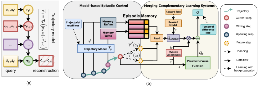
Figure 1: (a) Trajectorial Recall. The trajectory model reconstructs any past observation along the trajectory given noisy preceding s-a pair as a cue. (b) Dynamic hybrid control with the episodic memory at its core. The trajectory model, trained with TR loss (Eq. 1), encodes representations for writing (Eq. 2) and updating (Eq. 4) the episodic memory. Model-based Episodic Control (MBEC) plans actions (e.g. $a_{1}$ and $a_{2}$) and computes future trajectory representations ($\overrightarrow{\tau}^{\prime}\left(a_{1}\right)$ and $\overrightarrow{\tau}^{\prime}\left(a_{2}\right)$) for reading the memory’s stored values. The read-out, together with the reward model, estimates the episodic value $Q_{MBEC}$ (Eq. 6). The Complementary Learning Systems (CLS) combines $Q_{MBEC}$ and the traditional semantic $Q_{\theta}$ using dynamic consolidation conditioned on $\overrightarrow{\tau}$ (Eq. 7). The parameters of the CLS are optimized with TD loss (Eq. 8; habitual control).

We introduce a novel model that combines habitual, model based and episodic control wherein episodic memory plays a central role. Thanks to the memory storing trajectory representations, we can estimate the value in a model-driven fashion: for any action considered, the future trajectory is computed to query the episodic memory and get the action value. This takes advantage of model-based planning and episodic inference. The episodic value is then fused with a slower, parametric value function to leverage the capability of both episodic and habitual learning. Fig. 1 illustrates these components. We first present the formation of the trajectory representation and the episodic memory. Next, we describe how we estimate the value from this memory and parametric Q networks.

3.1 Episodic Memory Stores Trajectory Representations

In this paper, a trajectory $\tau_{t}$ is a sequence of what happens up to the time step $t$: $\tau_{t}=\left[(s_{1},a_{1}),...,(s_{t},a_{t})\right]$. If we consider $\tau_{t}$ as a piece of memory that encodes events in an episode, from that memory, we must be able to recall any past event. This ability in humans can be examined through the serial recall test wherein a previous item cues to the recall of the next item in a sequence farrell2012temporal . We aim to represent trajectories as vectors manifesting that property. As such, we employ a recurrent trajectory network $\mathcal{T}_{\phi}$ to model $\overrightarrow{\tau}_{t}=\mathcal{T_{\phi}}\left(\left[s_{t},a_{t}\right],\overrightarrow{\tau}_{t-1}\right)$ where $\mathcal{T}_{\phi}$ is implemented as an LSTM hochreiter1997long and $\overrightarrow{\tau}_{t}\in\mathbb{R}^{H}$ is the vector representation of $\tau_{t}$ and also the hidden state of the LSTM.

We train the trajectory model $\mathcal{T}_{\phi}$ to compute $\overrightarrow{\tau}_{t}$ such that it is able to reconstruct the next observation of any past experience, simulating the serial recall test. Concretely, given a noisy version $\left(\tilde{s}_{t^{\prime}},\tilde{a}_{t^{\prime}}\right)$ of a query state-action $\left(s_{t^{\prime}},a_{t^{\prime}}\right)$ sampled from a trajectory buffer $\mathcal{B}$ at time step $t^{\prime}<t$, we minimize the trajectorial recall (TR) loss as follows,

$$\mathcal{L}_{tr} =\mathbb{E}\left(\left\|y^{*}\left(t\right)-\left[s_{t^{\prime}+1},a_{t^{\prime}+1}\right]\right\|_{2}^{2}\right)$$ (1)

where $y^{*}\left(t\right)=\mathcal{G}_{\omega}\left(\mathcal{T_{\phi}}\left(\left[\tilde{s}_{t^{\prime}},\tilde{a}_{t^{\prime}}\right],\overrightarrow{\tau}_{t}\right)\right)$, $\mathcal{G}_{\omega}$ is a reconstruction function, implemented as a feed-forward neural network. The trajectory network $\mathcal{T}_{\phi}$ must implement some form of associative memory, compressing information of any state-action query in the past in its current representation $\overrightarrow{\tau}_{t}$ to reconstruct the next observation of the query, keeping the TR loss low (see a visualization in Fig. 1 (a)). Appendix A.1 theoretically explains why the TR loss is suitable for episodic control.

Our goal is to keep the trajectory representation and its associated value as the key and value of an episodic memory $\mathcal{M}=\left\{\mathcal{M}^{k},\mathcal{M}^{v}\right\}$, respectively. $\mathcal{M}^{k}\in\mathbb{R}^{N\times H}$ and $\mathcal{M}^{v}\in\mathbb{R}^{N\times 1}$, where $N$ is the maximum number of memory slots. The true value of a trajectory $\overrightarrow{\tau}_{t}$ is simply defined as the value of the resulting state of the trajectory $V\left(\overrightarrow{\tau}_{t}\right)=V\left(s_{t+1}\right)=\mathbb{E}\left(\sum_{i=0}^{T-t-1}\gamma^{i}r_{t+1+i}\right)$, $T$ is the terminal step. The memory stores estimation of the true trajectory values through averaging empirical returns by our weighted average writing mechanism (see in the next section).

1:$\mathcal{D}$: Replay buffer; $\mathcal{B}$: Trajectory buffer; $\mathcal{C}$: Chunk buffer; $\mathcal{M}$: Episodic memory; $\mathcal{T}_{\phi}$: Trajectory model; $r_{\varphi}\left(s,a\right)$: Reward model; $L$: Chunk length

2:for each episode do

3:     Initialize $\overrightarrow{\tau}_{0}=0$; $\mathcal{B}=\emptyset$; $\mathcal{C}=\emptyset$

4:     for $t=1,T$ do

5:         Observe state $s_{t}$. Compute $f_{\beta}\left(\overrightarrow{\tau}_{t-1}\right)$.

6:         Select action $a_{t}\leftarrow\epsilon$-greedy policy using Q in Eq. 7

7:         Observe reward $r_{t}$. Move to next state $s_{t+1}$. Compute $\overrightarrow{\tau}_{t}\leftarrow\mathcal{T_{\phi}}\left(\left[s_{t},a_{t}\right],\overrightarrow{\tau}_{t-1}\right)$

8:         Add ($s_{t},a_{t},s_{t+1},r_{t},\overrightarrow{\tau}_{t-1},\overrightarrow{\tau}_{t}$) and ($s_{t},a_{t}$) to $\mathcal{D}$ and $\mathcal{B}$, respectively.

9:         Refine memory: $\mathcal{M}\leftarrow\mathrm{refine}\left(s_{t},\overrightarrow{\tau}_{t-1}|\mathcal{M}\right)$

10:         for ($s_{t^{\prime}},a_{t^{\prime}},s_{t^{\prime}+1},r_{t^{\prime}},\overrightarrow{\tau}_{t^{\prime}-1},\overrightarrow{\tau}_{t^{\prime}}$) sampled from $\mathcal{D}$ do

11:              Compute $Q\left(s,a\right)$ using $s_{t^{\prime}},a_{t^{\prime}},\overrightarrow{\tau}_{t^{\prime}-1}$ (Eq. 7)

12:              Compute $Q\left(s^{\prime},a^{\prime}\right)$ using $s_{t^{\prime}+1},\overrightarrow{\tau}_{t^{\prime}}$ $\forall a^{\prime}$ (Eq. 7)

13:              Optimize $\mathcal{L}_{q}$ wrt $\theta$ and $\beta$ (Eq. 8)

14:              Compute $\mathcal{L}_{re}$ using $s_{t^{\prime}},a_{t^{\prime}},r_{t^{\prime}}$ (Eq. 5). Optimize $\mathcal{L}_{re}$ wrt $\varphi$          

15:         if $t\bmod L==0$ then

16:              Add ($\overrightarrow{\tau}_{t-1}$, $r_{t}$) to $\mathcal{C}$. Sample ($s_{t^{\prime}},a_{t^{\prime}}$) from $\mathcal{B}$ and optimize $\mathcal{L}_{tr}$ wrt $\phi$ and $\omega$ (Eq. $\ref{eq:trj_l})$          

17:         if $t==T$ then

18:              for each $\overrightarrow{\tau}_{i}\in\mathcal{C}$ do

19:                  Compute $\hat{V}\left(\overrightarrow{\tau}_{i}\right)=\sum_{j=i}^{T-1}\gamma^{j-i}r_{j+1}$. Write $\mathcal{M}\leftarrow\mathrm{\mathrm{write}}\left(\overrightarrow{\tau}_{i},\hat{V}\left(\overrightarrow{\tau}_{i}\right)|\mathcal{M}\right)$                             

Algorithm 1 MBEC++: Complementary reinforcement learning with MBEC and DQN.

3.2 Memory Operators

Memory reading Given a query key $\overrightarrow{\tau}$, we read from the memory the corresponding value by referring to neighboring representations. Concretely, two reading rules are employed

$$\mathrm{\mathrm{read}}\left(\overrightarrow{\tau}|\mathcal{M}\right) = \begin{cases}\sum_{i\in\mathcal{N}^{K_{r}}(\overrightarrow{\tau})}\frac{\left\langle\mathcal{M}_{i}^{k},\overrightarrow{\tau}\right\rangle\mathcal{M}_{i}^{v}}{\sum_{j\in\mathcal{N}^{K}(\overrightarrow{\tau})}\left\langle\mathcal{M}_{j}^{k},\overrightarrow{\tau}\right\rangle}&\left(a\right)\\ \max_{i\in\mathcal{N}^{K_{r}}(\overrightarrow{\tau})}\mathcal{M}_{i}^{v}&\left(b\right)\end{cases}$$

where $\left\langle\cdot\right\rangle$ is a kernel function and $\mathcal{N}^{K_{r}}\left(\cdot\right)$ retrieves top $K_{r}$ nearest neighbors of the query in $\mathcal{M}^{k}$. The read-out is an estimation of the value of the trajectory $\overrightarrow{\tau}$ wherein the weighted average rule $\left(a\right)$ is a balanced estimation, while the max rule $\left(b\right)$ is optimistic, encouraging exploitation of the best local experience. In this paper, the two reading rules are simply selected randomly with a probability of $p_{read}$ and $1-p_{read}$, respectively.

Memory writing Given the writing key $\overrightarrow{\tau}$ and its estimated value $\hat{V}\left(\overrightarrow{\tau}\right)$, the write operator $\mathrm{\mathrm{write}}\left(\overrightarrow{\tau},\hat{V}\left(\overrightarrow{\tau}\right)|\mathcal{M}\right)$ consists of several steps. First, we add the value to the memories $\mathcal{M}^{v}$ if the key cannot be found in the key memory $\mathcal{M}^{k}$ (this happens frequently since key match is rare). Then, we update the values of the key neighbors such that the updated values are approaching the written value $\hat{V}\left(\overrightarrow{\tau}\right)$ with speeds relative to the distances as $\forall i\in\mathcal{N}^{K_{w}}(\overrightarrow{\tau}):$

$$\mathcal{M}_{i}^{v} \leftarrow\mathcal{M}_{i}^{v}+\alpha_{w}\left(\hat{V}\left(\overrightarrow{\tau}\right)-\mathcal{M}_{i}^{v}\right)\frac{\left\langle\mathcal{M}_{i}^{k},\overrightarrow{\tau}\right\rangle}{\sum_{j\in\mathcal{N}^{K_{w}}(\overrightarrow{\tau})}\left\langle\mathcal{M}_{j}^{k},\overrightarrow{\tau}\right\rangle}$$ (2)

where $\alpha_{w}$ is the writing rate. Finally, the key can be added to the key memory. When it exceeds memory capacity $N$, the earliest added will be removed. For simplicity, $K_{w}=K_{r}=K$.

We note that our memory writing allows multiple updates to multiple neighbor slots, which is unlike the single-slot update rule blundell2016model ; pritzel2017neural ; lin2018episodic . Here, the written value is the Monte Carlo return collected from $t+1$ to the end of the episode $\hat{V}\left(\overrightarrow{\tau}_{t}\right)=\sum_{i=0}^{T-t-1}\gamma^{i}r_{t+1+i}$. Following le2019learning , we choose to write the trajectory representation of every $L$-th time-step (rather than every time-step) to save computation while still maintaining good memorization. Appendix A.2 provides a mean convergence analysis of our writing mechanism.

Memory refining As the memory writing is only executed after the episode ends, it delays the value propagation inside the memory. Hence, we design the $\mathrm{refine}\left(s_{t},\overrightarrow{\tau}_{t-1}|\mathcal{M}\right)$ operator that tries to minimize the one-step TD error of the memory’s value estimation. As such, at an arbitrary timestep $t$, we estimate the future trajectory if the agent takes action $a$ using the trajectory model as $\overrightarrow{\tau}_{t}^{\prime}\left(a\right)=\mathcal{T}_{\phi}\left(\left[s_{t},a\right],\overrightarrow{\tau}_{t-1}\right)$. Then, we can update the memory values as follows,

$$Q^{\prime}=\underset{a}{\max}\,r_{\varphi}\left(s_{t},a\right)+\gamma\mathrm{read}\left(\overrightarrow{\tau}_{t}^{\prime}\left(a\right)|\mathcal{M}\right)$$ (3)

$$\mathcal{M} \leftarrow\mathrm{write}\left(\overrightarrow{\tau}_{t-1},Q^{\prime}|\mathcal{M}\right)$$ (4)

where $r_{\varphi}$ is a reward model using a feed-forward neural network. $r_{\varphi}$ is trained by minimizing

$$\mathcal{L}_{re}=\mathbb{E}\left(r-r_{\varphi}\left(s,a\right)\right)^{2}$$ (5)

The memory refining process can be shown to converge in finite MDP environments.

Proposition 1.

In a finite MDP ($\mathcal{S}$,$\mathcal{A}$,$\mathcal{T}$,$\mathcal{R}$), given a fixed bounded $r_{\varphi}$ and an episodic memory $\mathcal{M}$ with $\mathrm{\mathrm{read}}$ (average rule) and $\mathrm{\mathrm{write}}$ operations, the memory $\mathrm{refine}$ given by Eq. 4 converges to a fixed point with probability 1 as long as $\gamma<1$, $\sum_{t=1}^{\infty}\alpha_{w,t}=\infty$ and $\sum_{t=1}^{\infty}\alpha_{w,t}^{2}<\infty$.

Proof.

See Appendix A.3. ∎

3.3 Model-based Episodic Control (MBEC)

Our agent relies on the memory at every timestep to choose its action for the current state $s_{t}$. To this end, the agent first plans some action and uses $\mathcal{T_{\phi}}$ to estimate the future trajectory. After that, it reads the memory to get the value of the planned trajectory. This mechanism takes advantage of model-based RL’s planning and episodic control’s non-parametric inference, yielding a novel hybrid control named Model-based Episodic Control (MBEC). The state-action value then is

$$Q_{MBEC}\left(s,a\right)=r_{\varphi}\left(s,a\right)+\gamma\mathrm{read}\left(\overrightarrow{\tau}^{\prime}\left(a\right)|\mathcal{M}\right)$$ (6)

The MBEC policy then is $\pi\left(s\right)=\underset{a}{\mathrm{argmax}}\>Q_{MBEC}\left(s,a\right)$. Unlike model-free episodic control, we compute on-the-fly instead of storing the state-action value. Hence, the memory does not need to store all actions to get reliable action values.

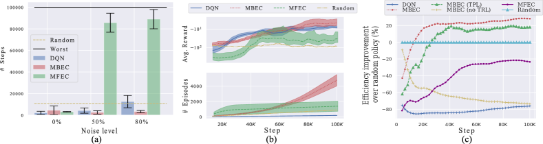
Figure 2: Maze navigation. (a) Noisy mode: number of steps required to complete 100 episodes with different noise rates (lower is better). (b) Trap mode: average reward (upper) and number of completed episodes (lower) over timesteps (higher is better). (c) Dynamic mode: efficiency improvement over random policy across timesteps (higher is better).

3.4 Model-based Episodic Control Facilitates Complementary Learning Systems

The episodic value provides direct yet biased estimation from experiences. To compensate for that, we can use a neural network $Q_{\theta}\left(s_{t},a_{t}\right)$ to give an unbiased value estimation mnih2015human , representing the slow-learning semantic memory that gradually encodes optimal values. Prior works combine by a weighted summation of the episodic and semantic value wherein the weight is fixed lin2018episodic ; hansen2018fast . We believe that depending on the specific observations, we may need different weights to combine the two values. Hence, we propose to combine the two episodic and semantic systems as

$$Q\left(s_{t},a_{t}\right)=Q_{MBEC}\left(s_{t},a_{t}\right)f_{\beta}\left(\overrightarrow{\tau}_{t-1}\right)+Q_{\theta}\left(s_{t},a_{t}\right)$$ (7)

where $f_{\beta}$ is a feed-forward neural network with sigmoid activation that takes the previous trajectory as the input and outputs a consolidating weight for the episodic value integration. This allows dynamic integration conditioned on the trajectory status. The semantic system learns to take episodic estimation into account in making decisions via replaying to minimize one-step TD error,

$$\mathcal{L}_{q}=\mathbb{E}\left(r+\gamma\max_{a^{\prime}}Q\left(s^{\prime},a^{\prime}\right)-Q\left(s,a\right)\right)^{2}$$ (8)

Here we note that $Q_{MBEC}$ is also embedded in the target, providing better target value estimation in the early phase of learning when the parametric model does not learn well. We follow mnih2015human using a replay buffer $\mathcal{D}$ to store $\left(s,a,s^{\prime},r\right)$ across episodes. Without episodic contribution, TD or habitual learning is slow hansen2018fast ; lin2018episodic . Our episodic integration allows the agent to rely on MBEC whenever it needs to compensate for immature parametric systems. Alg. 1 (MBEC++) summarizes MBEC operations within the complementary learning system. The two components (MBEC and CLS) are linked by the episodic memory as illustrated in Fig. 1 (b).

4 Results

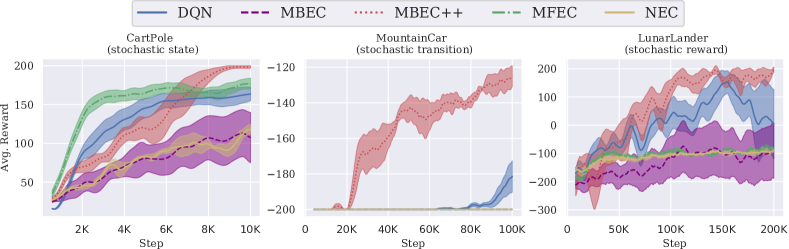
Figure 3: Average reward over learning steps on representative stochastic classical control environments (higher is better, mean and std. over 10 runs).

In this section, we examine our proposed episodic control both as a stand-alone (MBEC) and within a complementary learning system (MBEC++). To keep our trajectory model simple, for problems with image state, it learns to reconstruct the feature vector of the image input, rather than the image itself. The main baselines are DQN mnih2015human and recent (hybrid) episodic control methods. Details of the baseline configurations and hyper-parameter tuning for each tasks can be found in Appendix B.

4.1 Grid-world: 2D Maze Exploration

We begin with simple maze navigation to explore scenarios wherein our proposed memory shows advantages. In this task, an agent is required to move from the starting point $\left(0,0\right)$ to the endpoint $\left(n_{e}-1,n_{e}-1\right)$ in a maze environment of size $n_{e}\times n_{e}$. In the maze task, if the agent hits the wall of the maze, it gets $-1$ reward. If it reaches the goal, it gets $+1$ reward. For each step in the maze, the agent get $-0.1/n_{e}^{2}$ reward. An episode ends either when the agent reaches the goal or the number of steps exceeds 1000. We create different scenarios for this task ($n_{e}=3$): noisy, trap and dynamic modes wherein our MBEC is compared with both parametric (DQN) and memory-based (MFEC; blundell2016model ) models (see Appendix B.2 for details and more results).

Noisy mode In this mode, the state is represented as the location plus an image of the maze. The image is preprocessed by a pretrained ResNet, resulting in a feature vector of $512$ dimensions (the output layer before softmax). We apply dropout to the image vector with different noise levels. We hypothesize that aggregating states into trajectory representation as in MBEC is a natural way to smooth out the noise of individual states.

Fig. 2 (a) measures sample efficiency of the models on noisy mode. Without noise, all models can quickly learn the optimal policy and finish 100 episodes within 1000 environment steps. However, as the increased noise distracts the agents, MFEC cannot find a way out until the episode ends. DQN performance reduces as the noise increases and ends up even worse than random exploration. By contrast, MBEC tolerates noise and performs much better than DQN and the random agent.

Trap mode The state is the position of the agent plus a trap location randomly determined at the beginning of the episode. If the agent falls into the trap, it receives a $-2$ reward (the episode does not terminate). This setting illustrates the advantage of memory-based planning. With MBEC, the agent remembers to avoid the trap by examining the future trajectory to see if it includes the trap. Estimating state-action value (DQN and MFEC) introduces overhead as they must remember all state-action pairs triggering the trap.

We plot the average reward and number of completed episodes over time in Fig. 2 (b). In this mode, DQN always learns a sub-optimal policy, which is staying in the maze. It avoids hitting the wall and trap, however, completes a relatively low number of episodes. MFEC initially learns well, quickly completing episodes. However its learning becomes unstable as more observations are written into its memory, leading to a lower performance over time. MBEC alone demonstrates stable learning, significantly outperforming other baselines in both reward and sample efficiency.

Dynamic mode The state is represented as an image and the maze structure randomly changes for each episode. A learnable CNN is equipped for each baseline to encode the image into a $64$-dimensional vector. In this dynamic environment, similar state-actions in different episodes can lead to totally different outcomes, thereby highlighting the importance of trajectory modeling. In this case, MFEC uses VAE-CNN, trained to reconstruct the image state. Also, to verify the contribution of TR loss, we add two baselines: (i) MBEC without training trajectory model (no TRL) and (ii) MBEC with a traditional model-based transition prediction loss (TPL) (see Appendix B.2 for more details).

We compare the models’ efficiency improvement over random policy by plotting the percentage of difference between the models’ number of finished episodes and that of random policy in Fig. 2 (c). DQN and MFEC perform worse than random. MBEC with untrained trajectory model performs poorly. MBEC with trajectory model trained with TPL shows better performance than random, yet still underperforms our proposed MBEC with TRL by around 5-10%.

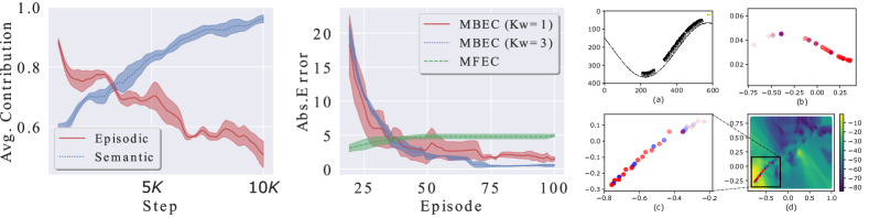
Figure 4: Cart Pole. (Left) Average contribution of episodic and semantic value estimations over timesteps (see Appendix B.3 for contribution definition). The episodic influence is gradually replaced by the semantic’s. (Middle) The difference (absolute error) between the stored and true value of the starting state (mean and std. over 5 runs). (Right) Mountain Car. (a) Visualization of the car moving uphill over 30 timesteps. Due to noise, the next state can be observed as the current state with probability $p_{tr}$. (b) State and (c) trajectory spaces: the axes are the dimension of the trajectory vectors $\vec{\tau}$ projected into 2d space. Blue denotes the representation at noisy timestep and red the normal ones. Fading color denotes earlier timesteps. (d) Value estimation by the episodic memory for the whole $2$-d trajectory space.

4.2 Stochastic Classical Control

In stochastic environments, taking correct actions can still lead to low rewards due to noisy observations, which negatively affects the quality of episodic memory. We consider 3 classical problems: Cart Pole, Mountain Car and Lunar Lander. For each problem, we examine RL agents in stochastic settings by (i) perturbing the reward with Gaussian (mean 0, std. $\sigma_{re}=0.2$) or (ii) Bernoulli noise (with probability $p_{re}=0.2$, the agent receives a reward $-r$ where $r$ is the true reward) and (iii) noisy transition (with probability $p_{tr}=0.5$, the agent observes the current state as its next state despite taking any action). In this case, we compare MBEC++ with DQN, MFEC and NEC pritzel2017neural .

Fig. 3 shows the performances of the models on representative environments (full results in Appendix B.3). For easy problems like Cart Pole, although MFEC learns quickly, its over-optimistic control is sub-optimal in non-deterministic environments, and thus cannot solve the task. For harder problems, stochasticity makes state-based episodic memories (MFEC, NEC) fail to learn. DQN learns in these settings, albeit slowly, illustrating the disadvantage of not having a reliable episodic memory. Among all, MBEC++ is the only model that can completely solve the noisy Cart Pole within 10,000 steps and demonstrates superior performance in Mountain Car and Lunar Lander. Compared to MBEC++, MBEC performs badly, showing the importance of CLS.

Behavior analysis The episodic memory plays a role in MBEC++’s success. In the beginning, the agent mainly relies on the memory, yet later, it automatically learns to switch to the semantic value estimation (see Fig. 4 (left)). That is because in the long run the semantic value is more reliable and already fused with the episodic value through Eq. 7-8. Our $\mathrm{write}$ operator also helps MBEC++ in quickly searching for the optimal value. To illustrate that, we track the convergence of the episodic memory’s written values for the starting state of the stochastic Cart Pole problem under a fixed policy (Fig. 4 (middle)). Unlike the over-optimistic MFEC’s writing rule using $\max$ operator, ours enables mean convergence to the true value despite Gaussian reward noise. When using a moderate $K_{w}>1$, the estimated value converges better as suggested by our analysis in Appendix A.2. Finally, to verify the contribution of the trajectory model, we examine MBEC++’s ability to counter noisy transition by visualizing the trajectory spaces for Mountain Car in Fig. 4 (right). Despite the noisy states (Fig. 4 (right, b)), the trajectory model can still roughly estimate the trace of trajectories (Fig. 4 (right, c)). That ensures when the agent approaches the goal, the trajectory vectors smoothly move to high-value regions in the trajectory space (Fig. 4 (right, d)). We note that for this problem that ability is only achieved through training with TR loss (comparison in Appendix B.3).

Ablation study We pick the noisy transition Mountain Car problem for ablating components and hyper-parameters of MBEC++ with different neighbors ($K$), chunk length ($L$) and memory slots ($N$). The results in Fig. 5 demonstrate that the performance improves as $K$ increases, which is common for KNN-based methods. We also find that using a too short or too long chunk deteriorates the performance of MBEC++. Short chunk length creates redundancy as the stored trajectories will be similar while long chunk length makes minimizing TR loss harder. Finally, the results confirm that the learning of MBEC++ is hindered significantly with small memory. A too-big memory does not help either since the trajectory model continually refines the trajectory representation, a too big memory slows the replacement of old representations with more accurate newer ones.

We also ablate MBEC++: (i) without TR loss, (ii) with TP loss (iii), without multiple write ($K_{w}=1$) and (iv) without memory $\mathrm{update}$. We realize that the first two configurations show no sign of learning. The last two can learn but much slower than the full MBEC++, justifying our neighbor memory writing and update (Fig. 5 (rightmost)). More ablation studies are in Appendix B.6 where we find our dynamic consolidation is better than fixed combinations and optimal $p_{read}$ is 0.7.

Model	All	25 games
Nature DQN	15.7/51.3	83.6/16.0
MFEC	85.0/45.4	77.7/40.9
NEC	99.8/54.6	106.1/53.3
EMDQN*	528.4/92.8	250.6/95.5
EVA	-	172.2/39.2
ERLAM	-	515.4/103.5
MBEC++	654.0/117.2	518.2/133.4

Table 1: Human normalized scores (mean/median) at 10 million frames for all and a subset of 25 games. Baselines’ numbers are adopted from original papers and zhu2019episodic , respectively. * The baseline is reported with 40 million frames of training. - The exact numbers are not reported.

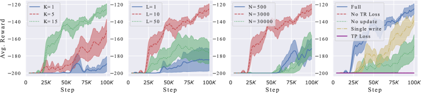
Figure 5: Noisy Transition Mountain Car: ablation study. Each plot varies one hyper-parameter or ablated component while fixing others in default values ($K=15$, $L=10$, $N=3000$).

4.3 Atari 2600 Benchmark

We benchmark MBEC++ against other strong episodic memory models in playing Atari 2600 video games bellemare2013arcade . The task can be challenging with stochastic and partially observable games kaiser2019model . Our model adopts DQN mnih2015human with the same setting (details in Appendix B.4). We only train the models within 10 million frames for sample efficiency.

Table 1 reports the average performance of MBEC++ and baselines on all (57) and 25 popular Atari games concerning human normalized metrics mnih2015human . Compared to the vanilla DQN, MFEC and NEC, MBEC++ is significantly faster at achieving high scores in the early learning phase. Further, MBEC++ outperforms EMDQN even trained with 40 million frames and achieves the highest median score. Here, state-action value estimations fall short in quickly solving complicated tasks with many actions like playing Atari games as it takes time to visit enough state-action pairs to create useful memory’s stored values. By contrast, when the models in MBEC++ are well-learnt (which is often within 5 million frames, see Appendix B.4), its memory starts providing reliable trajectory value estimation to guide the agent to good policies. Remarkably, our episodic memory is much smaller than that of others and our trajectory model size is insignificant to DQN’s (Appendix B.4 and Table 2).

In the subset testbed, MBEC++ demonstrates competitive performance against trajectory-utilized models including EVA hansen2018fast and ERLAM zhu2019episodic . These baselines work with trajectories as raw state-action sequences, unlike our distributed trajectories. In the mean score metric, MBEC++ is much better than EVA (nearly double score) and slightly better than ERLAM. MBEC++ agent plays consistently well across games without severe fluctuations in performance, indicated by its significantly higher median score.

We also compare MBEC++ with recent model-based RL approaches including Dreamer-v2 hafner2020mastering and SIMPLE kaiser2019model . The results show that our method is competitive against these baselines. Notably, our trajectory model is much simpler than the other methods (we only have TR and reward losses and our network is the standard CNN of DQN for Atari games). Appendix B.4 provides more details, learning curves and further analyses.

4.4 POMDP: 3D Navigation

To examine MBEC++ on Partially-Observable Markov Decision Process (POMDP) environments, we conduct experiments on a 3D navigation task: Gym Mini-World’s Pickup Objects gym_miniworld . Here, an agent moves around a big room to collect several objects ($+1$ reward for each picked object). The location, shape and color of the objects change randomly across episodes. The state is the frontal view-port of the agent and encoded by a common CNN for all baselines (details in Appendix B.5).

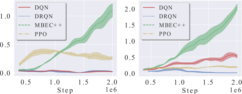
Figure 12: 3D Navigation. Average reward for picking 3 (left) and 5 (right) objects over environment steps (mean and std. over 5 runs).

We train all models for only 2 million steps and report the results for a different number of objects in Appendix’s Fig. 12. Among all baselines, MBEC++ demonstrates the best learning progress and consistently improves over time. Other methods either fail to learn (DRQN) or show a much slower learning speed (DQN and PPO). That proves our MBEC++ is useful for POMDP.

5 Conclusion

We have introduced a new episodic memory that significantly accelerates reinforcement learning in various problems beyond near-deterministic environments. Its success can be attributed to: (a) storing distributed trajectories produced by a trajectory model, (b) memory-based planning with fast value-propagating memory writing and refining, and (c) dynamic consolidation of episodic values to parametric value function. Our experiments demonstrate the superiority of our method to prior episodic controls and strong RL baselines. One limitation of this work is the large number of hyperparameters, which prevents us from fully tuning MBEC++. In future work, we will extend to continuous action space and explore multi-step memory-based planning capability of our approach.

Our research aims to improve sample-efficiency of RL and can be trained with common computers. Our method improves the performance in various RL tasks, and thus opens the chance for creating better autonomous systems that work flexibly across sectors (robotics, manufacturing, logistics, and decision support systems). Although we do not think there are immediate bad consequences, we are aware of potential problems. First, our method does not guarantee safe exploration during training. If learning happens in a real-world setting (e.g. self-driving car), the agent can make unsafe exploration (e.g. causing accidents). Second, we acknowledge that our method, like many other Machine Learning algorithms, can be misused in unethical or malicious activities.

ACKNOWLEDGMENTS

This research was partially funded by the Australian Government through the Australian Research Council (ARC). Prof Venkatesh is the recipient of an ARC Australian Laureate Fellowship (FL170100006).

Appendix

A Analytical Studies on Model-based Episodic Memory

A.1 Why Is Trajectorial Recall (TR) Loss Good for Episodic Memory?

For proper episodic control, neighboring keys should represent similar trajectories. If we simply assume that two trajectories are similar if they share many common transitions, training the trajectory model with TR loss indeed somehow enforces that property. To illustrate, we consider simple linear $\mathcal{T_{\phi}}$ and $\mathcal{G}_{\omega}$ such that the reconstruction process becomes

$$y^{*}\left(t\right)=W\left(U\overrightarrow{\tau}_{t}+V\left[s_{t^{\prime}},a_{t^{\prime}}\right]\right)$$

Here, we also assume that the query is clean without added noise. Then we can rewrite TR loss for a trajectory $\tau_{t}$

$$\mathcal{L}_{tr}\left(\tau_{t}\right) =\sum_{t^{\prime}=1}^{t}\left\|W\left(U\overrightarrow{\tau}_{t}+V\left[s_{t^{\prime}},a_{t^{\prime}}\right]\right)-\left[s_{t^{\prime}+1},a_{t^{\prime}+1}\right]\right\|_{2}^{2}$$

$$=\sum_{t^{\prime}=1}^{t}\left\|\Delta_{t^{\prime}}\left(\tau_{t}\right)\right\|_{2}^{2}$$

Let us denote $S\neq\emptyset$ the set of common transition steps between 2 trajectories: $\tau_{t_{1}}^{1}$ and $\tau_{t_{2}}^{2}$, by applying triangle inequality,

$$\mathcal{L}_{tr}\left(\tau_{t_{1}}^{1}\right)+\mathcal{L}_{tr}\left(\tau_{t_{2}}^{2}\right) \geq\sum_{t^{\prime}\in S}\left\|\Delta_{t^{\prime}}\left(\tau_{t_{1}}^{1}\right)\right\|_{2}^{2}+\left\|\Delta_{t^{\prime}}\left(\tau_{t_{2}}^{2}\right)\right\|_{2}^{2}$$

$$\geq\sum_{t^{\prime}\in S}\left\|\Delta_{t^{\prime}}\left(\tau_{t_{1}}^{1}\right)-\Delta\left(\tau_{t_{2}}^{2}\right)\right\|_{2}^{2}$$

$$=\left|S\right|\left\|WU\left(\overrightarrow{\tau}_{t_{1}}^{1}-\overrightarrow{\tau}_{t_{2}}^{2}\right)\right\|_{2}^{2}$$

If we assume $WU\left(\overrightarrow{\tau}_{t_{1}}^{1}-\overrightarrow{\tau}_{t_{2}}^{2}\right)\neq 0$ as $\overrightarrow{\tau}_{t_{1}}^{1}\neq\overrightarrow{\tau}_{t_{2}}^{2}$, applying Lemma 2.3 in [12] yields

$$\frac{\mathcal{L}_{tr}\left(\tau_{t_{1}}^{1}\right)+\mathcal{L}_{tr}\left(\tau_{t_{2}}^{2}\right)}{\left|S\right|\sigma_{min}\left(WU\right)}\geq\left\|\overrightarrow{\tau}_{t_{1}}^{1}-\overrightarrow{\tau}_{t_{2}}^{2}\right\|_{2}^{2}$$

where $\sigma_{min}\left(WU\right)$ is the smallest nonzero singular value of $WU$. As the TR loss decreases and the number of common transition increases, the upper bound of the distance between two trajectory vectors decreases, which is desirable. On the other hand, it is unclear whether the traditional transition prediction loss holds that property.

A.2 Convergence Analysis of $\mathrm{write}$ Operator

In this section, we show that we can always find $\alpha_{w}$ such that the writing converges with probability $1$ and analyze the convergence as $\alpha_{w}$ is constant. To simplify the notation, we rewrite Eq. 2 as

$$\mathcal{M}_{i}^{v}\left(n+1\right)=\mathcal{M}_{i}^{v}\left(n\right)+\text{$\lambda\left(n\right)$}\left(R_{j}\left(n\right)-\mathcal{M}_{i}^{v}\left(n\right)\right)$$ (9)

where $i$ and $j$ denote the current memory slot being updated and its neighbor that initiates the writing, respectively. $\lambda\left(n\right)=\alpha_{w}\left(n\right)\frac{\left\langle\right\rangle_{ij}\left(n\right)}{\sum_{b\in\mathcal{N}_{j}^{K_{w}}}\left\langle\right\rangle_{bj}\left(n\right)}$ where $\mathcal{N}_{j}^{K_{w}}$ is the set of $K_{w}$ neighbors of $j$. $R_{j}$ is the empirical return of the trajectory whose key is the memory slot $j$, $\left\langle\right\rangle_{ij}$ the kernel function of 2 keys and $n$ the number of updates. As mentioned in [40], this stochastic approximation converges when $\sum_{n=1}^{\infty}\lambda\left(n\right)=\infty$ and $\sum_{n=1}^{\infty}\lambda^{2}\left(n\right)<\infty$.

By definition, $\left\langle\right\rangle_{ij}=\frac{1}{\left\|\overrightarrow{\tau}_{i}-\overrightarrow{\tau}_{j}\right\|+\epsilon}$ and $\left\|\overrightarrow{\tau}\right\|\leq 1$ since $\overrightarrow{\tau}$ is the hidden state of an LSTM. Hence, we have $\forall i,j$: $0<\frac{1}{2+\epsilon}\leq\left\langle\right\rangle_{ij}\leq\frac{1}{\epsilon}$. Hence, let $B_{ij}\left(n\right)$ a random variable denoting $\frac{\left\langle\right\rangle_{ij}\left(n\right)}{\sum_{b\in\mathcal{N}_{j}^{K_{w}}}\left\langle\right\rangle_{bj}\left(n\right)}$–the neighbor weight at step $n$, $\forall i,j:$

$$\frac{\epsilon}{K_{w}\epsilon+2K_{w}-2}\leq B_{ij}\left(n\right)\leq\frac{2+\epsilon}{K_{w}\epsilon+2}$$

That yields $\sum_{n=1}^{\infty}\lambda\left(n\right)\geq\frac{\epsilon}{K_{w}\epsilon+2K-2}\sum_{n=1}^{\infty}\alpha_{w}\left(n\right)$ and $\sum_{n=1}^{\infty}\lambda^{2}\left(n\right)\leq\left(\frac{2+\epsilon}{K_{w}\epsilon+2}\right)^{2}\sum_{n=1}^{\infty}\alpha_{w}^{2}\left(n\right)$. Hence the writing updates converge when $\sum_{n=1}^{\infty}\alpha_{w}\left(n\right)=\infty$ and $\sum_{n=1}^{\infty}\alpha_{w}^{2}\left(n\right)<\infty$. We can always choose such $\alpha_{w}$ (e.g., $\alpha_{w}\left(n\right)=\frac{1}{n+1}$).

With a constant writing rate $\alpha$, we rewrite Eq. 9 as

$$\mathcal{M}_{i}^{v}\left(n+1\right) =\mathcal{M}_{i}^{v}\left(n\right)+\alpha B_{ij}\left(n\right)\left(R_{j}\left(n\right)-\mathcal{M}_{i}^{v}\left(n\right)\right)$$

$$=\alpha B_{ij}\left(n\right)R_{j}\left(n\right)+\text{$\mathcal{M}_{i}^{v}\left(n\right)\left(1-\alpha B_{ij}\left(n\right)\right)$}$$

$$=\sum_{t=1}^{n}\alpha B_{ij}\left(t\right)\prod_{l=t+1}^{n}\left(1-\alpha B_{ij}\left(l\right)\right)R_{j}\left(t\right)$$

$$+\prod_{t=1}^{n}\left(1-\alpha B_{ij}\left(t\right)\right)\mathcal{M}_{i}^{v}\left(1\right)$$

where the second term $\prod_{t=1}^{n}\left(1-\alpha B_{ij}\left(t\right)\right)\mathcal{M}_{i}^{v}\left(1\right)\rightarrow 0$ as $n\rightarrow\infty$ since $B_{ij}\left(t\right)$ and $\alpha$ are bounded between 0 and 1. The first term can be decomposed into three terms

$$\sum_{t=1}^{n}\alpha B_{ij}\left(t\right)\prod_{l=t+1}^{n}\left(1-\alpha B_{ij}\left(l\right)\right)R_{j}\left(t\right) =T_{1}+T_{2}+T_{3}$$

where

$$T_{1} =\sum_{t=1}^{n}\alpha B_{ij}\left(t\right)\prod_{l=t+1}^{n}\left(1-\alpha B_{ij}\left(l\right)\right)V_{i}$$

$$T_{2} =\sum_{t=1}^{n}\alpha B_{ij}\left(t\right)\prod_{l=t+1}^{n}\left(1-\alpha B_{ij}\left(l\right)\right)\Delta V_{ij}\left(t\right)$$

$$T_{3} =\sum_{t=1}^{n}\alpha B_{ij}\left(t\right)\prod_{l=t+1}^{n}\left(1-\alpha B_{ij}\left(l\right)\right)\tilde{R}_{j}\left(t\right)$$

Here,$V_{i}$ is the true value of the trajectory stored in slot $i$, $\Delta V_{ij}\left(t\right)=V_{j}\left(t\right)-V_{i}$ and $\tilde{R}_{j}\left(t\right)=R_{j}\left(t\right)-V_{j}\left(t\right)$ the noise term between the return and the true value. Assume that the value is associated with zero mean noise and the value noise is independent with the neighbor weights, then $\mathbb{E}\left(T_{3}\right)=0$.

Further, we make other two assumptions: (1) the neighbor weights are independent across update steps; (2) the probability $p_{j}$ of visiting a neighbor $j$ follows the same distribution across update steps and thus, $\mathbb{E}\left(B_{ij}\left(t\right)\right)=\mathbb{E}\left(B_{ij}\left(l\right)\right)=\mathbb{E}\left(B_{ij}\right)$. We now can compute

$$\mathbb{E}\left(T_{1}\right) =\mathbb{E}\left(\sum_{t=1}^{n}\alpha B_{ij}\left(t\right)\prod_{l=t+1}^{n}\left(1-\alpha B_{ij}\left(l\right)\right)V_{i}\right)$$

$$=V_{i}\sum_{t=1}^{n}\alpha\mathbb{E}\left(B_{ij}\right)\prod_{l=t+1}^{n}\left(1-\alpha\mathbb{E}\left(B_{ij}\right)\right)$$

$$=V_{i}\alpha\mathbb{E}\left(B_{ij}\right)\sum_{t=1}^{n}\left(1-\alpha\mathbb{E}\left(B_{ij}\right)\right)^{n-t}$$

$$=V_{i}\alpha\mathbb{E}\left(B_{ij}\right)\frac{1-\left(1-\alpha\mathbb{E}\left(B_{ij}\right)\right)^{n}}{1-\left(1-\alpha\mathbb{E}\left(B_{ij}\right)\right)}$$

$$=V_{i}\left(1-\left(1-\alpha\mathbb{E}\left(B_{ij}\right)\right)^{n}\right)$$

As $n\rightarrow\infty$, $\mathbb{E}\left(T_{1}\right)\rightarrow V_{i}$ since since $B_{ij}\left(t\right)$ and $\alpha$ are bounded between 0 and 1.

Similarly, $\mathbb{E}\left(T_{3}\right)=\mathbb{E}\left(V_{j}\left(t\right)-V_{i}\right)=\mathbb{E}\left(V_{j}\left(t\right)\right)-V_{i}=\sum_{j\in\mathcal{N}_{i}^{K_{w}}}p_{j}V_{j}-V_{i}$, which is the approximation error of the KNN algorithm. Hence, with constant learning rate, on average, the $\mathrm{write}$ operator leads to the true value plus the approximation error of KNN. The quality of KNN approximation determines the mean convergence of $\mathrm{write}$ operator. Since the bias-variance trade-off of KNN is specified by the number of neighbors $K$, choosing the right $K>1$ (not too big, not too small) is important to achieve good writing to ensure fast convergence. That explains why our writing to multiple slots ($K>1$) is generally better than the traditional writing to single slot ($K=1$).

A.3 Convergence Analysis of $\mathrm{refine}$ Operator

In this section, we study the convergence of the memory-based value estimation by applying $\mathrm{refine}$ operator to the memory. As such, we treat the $\mathrm{read}\left(\overrightarrow{\tau}|\mathcal{M}\right)$ operator as a value function over trajectory space $\mathcal{T}$ and simplify the notation as $\mathrm{read}\left(x\right)$ where $x$ represents the trajectory. We make the assumption that the $\mathrm{read}$ operator simply uses averaging rule and the set of neighbors stored in the memory is fixed (i.e. no new element is added to the memory) , then

$$\mathrm{\mathrm{read}}_{t}\left(x\right) = \sum_{i\in\mathcal{N}^{K}(x)}B_{ix}\mathcal{M}_{i,t}^{v}$$

where $B_{ix}=\frac{\left\langle\mathcal{M}_{i}^{k},x\right\rangle}{\sum_{j\in\mathcal{N}^{K}\left(x\right)}\left\langle\mathcal{M}_{j}^{k},x\right\rangle}$ is the neighbor weight and $t$ is the step of updating.

We rewrite the $\mathrm{refine}$ operator as

$$\mathcal{M} \leftarrow\mathrm{write}\left(x,\underset{a}{\max}\,r_{\varphi}\left(x,a\right)+\gamma\mathrm{read}_{t}\left(y\right)|\mathcal{M}\right)$$

$$\Leftrightarrow\forall i\in\mathcal{N}^{K}(x) :$$

$$\mathcal{M}_{i,t+1}^{v} =\mathcal{M}_{i,t}^{v}$$

$$+\alpha_{w,t}B_{ix}\left(\underset{a}{\max}\,r_{\varphi}\left(x,a\right)+\gamma\mathrm{read}_{t}\left(y\right)-\mathcal{M}_{i,t}^{v}\right)$$

where $y$ is the trajectory after taking action $a$ from the trajectory $x$. Then, after the $\mathrm{refine}$,

$$\mathrm{\mathrm{read}}_{t+1}\left(x\right) = \sum_{i\in\mathcal{N}^{K}(x)}B_{ix}\mathcal{M}_{i,t+1}^{v}$$

$$= \sum_{i\in\mathcal{N}^{K}(x)}\mathcal{M}_{i,t}^{v}B_{ix}\left(1-\alpha_{w,t}\right)$$

$$+\alpha_{w,t}\sum_{i\in\mathcal{N}^{K}(x)}\left(\underset{a}{\max}\,r_{\varphi}\left(x,a\right)+\gamma\mathrm{read}_{t}\left(y\right)\right)B_{ix}^{2}$$

$$+\alpha_{w,t}\sum_{i\in\mathcal{N}^{K}(x)}\mathcal{M}_{i,t}^{v}B_{ix}\left(1-B_{ix}\right)$$

$$= \mathrm{\mathrm{read}}_{t}\left(x\right)\left(1-\alpha_{w,t}\right)+\alpha_{w,t}G_{t}\left(x\right)$$

where $G_{t}\left(x\right)=\underset{a}{\max}\,U_{t}\left(x,a\right)\sum_{i\in\mathcal{N}^{K}(x)}B_{ix}^{2}+\sum_{i\in\mathcal{N}^{K}(x)}\mathcal{M}_{i,t}^{v}B_{ix}\left(1-B_{ix}\right)$, $U\left(x,a\right)=r_{\varphi}\left(x,a\right)+\gamma\mathrm{read}\left(y\right)$. To simplify the analysis, we assume the stored neighbors of $x$ are apart from $x$ by the same distance, i.e., $\forall i\in\mathcal{N}^{K}(x):B_{ix}=\frac{1}{K}$. That is,

$$G\left(x\right)=\left(\underset{a}{\max}\,r_{\varphi}\left(x,a\right)+\gamma\mathrm{read}\left(y\right)\right)\frac{1}{K}+\mathrm{read}\left(x\right)\frac{K-1}{K}$$

Let $\mathrm{H}$ an operator defined for the function $\mathrm{read}:\mathcal{T\rightarrow}\mathbb{R}$ as

$$\mathrm{H}\mathrm{read}\left(x\right) =\sum_{\hat{y}\in\mathcal{T}}P_{a^{*}}\left(x,y\right)G_{t}\left(x|a^{*}\right)$$

where $a^{*}=\underset{a}{\mathrm{argmax}}\sum_{\hat{y}\in\mathcal{T}}P_{a}\left(x,y\right)U\left(x,a\right)$. We will prove $\mathrm{H}$ is a contraction in the sup-norm.

Let us denote $\Delta\mathrm{read}\left(x\right)=\mathrm{read}_{1}\left(x\right)-\mathrm{read}_{2}\left(x\right)$, $\Delta PU\left(x,a_{1}^{*},a_{2}^{*}\right)=\sum_{y\in\mathcal{T}}P_{a_{1}^{*}}\left(x,y\right)U_{1}\left(x,a_{1}^{*}\right)$ $-\sum_{y\in\mathcal{T}}P_{a_{2}^{*}}\left(x,y\right)U_{2}\left(x,a_{2}^{*}\right)$ and $\hat{a}=\underset{a_{1}^{*},a_{2}^{*}}{\mathrm{argmax}}\sum_{y\in\mathcal{T}}P_{a_{1}^{*}}\left(x,y\right)U_{1}\left(x,a_{1}^{*}\right)$, $\sum_{y\in\mathcal{T}}P_{a_{2}^{*}}\left(x,y\right)U_{2}\left(x,a_{2}^{*}\right)$. Then,

$$\left\|\mathrm{H}\mathrm{read}_{1}-\mathrm{H}\mathrm{read}_{2}\right\|_{\infty} =\left\|\sum_{y\in\mathcal{T}}\left(\Delta PU\left(x,a_{1}^{*},a_{2}^{*}\right)\frac{1}{K}\right.\right.$$

$$+\left.\left.\Delta\mathrm{read}\left(x\right)\frac{K-1}{K}\right)\right\|_{\infty}$$

$$\leq\left\|\sum_{y\in\mathcal{T}}\Delta PU\left(x,a_{1}^{*},a_{2}^{*}\right)\frac{1}{K}\right\|_{\infty}$$

$$+\left\|\frac{K-1}{K}\Delta\mathrm{read}\left(x\right)\right\|_{\infty}$$

$$\leq\left\|\sum_{y\in\mathcal{T}}\frac{P_{\hat{a}}\left(x,y\right)}{K}\gamma\Delta\mathrm{read}\left(y\right)\right\|_{\infty}$$

$$+\left\|\frac{K-1}{K}\Delta\mathrm{read}\left(x\right)\right\|_{\infty}$$

$$\leq\sum_{y\in\mathcal{T}}\frac{P_{\hat{a}}\left(x,y\right)}{K}\gamma\left\|\Delta\mathrm{read}\left(y\right)\right\|_{\infty}$$

$$+\left\|\frac{K-1}{K}\Delta\mathrm{read}\right\|_{\infty}$$

$$\leq\frac{\gamma+K-1}{K}\left\|\mathrm{read}_{1}-\mathrm{read}_{2}\right\|_{\infty}$$

Since $\gamma<1$, $0<\gamma_{K}=\frac{\gamma+K-1}{K}<1\>\forall K\geq 1$. Thus, $\mathrm{H}$ is a contraction in the sup-norm and there exists a fix-point $\mathrm{read}^{*}$ such that $\mathrm{H}\mathrm{read}^{*}=\mathrm{read}^{*}$.

We define $\Delta_{t}=\mathrm{read}_{t}-\mathrm{read}^{*}$, then

$$\Delta_{t+1}=\Delta_{t}\left(x\right)\left(1-\alpha_{w,n}\right)+\alpha_{w,t}F_{t}\left(x\right)$$

where $F_{t}\left(x\right)=G_{t}\left(x\right)-\mathrm{read}^{*}\left(x\right)$. We have

$$\mathbb{E}\left(F_{t}\left(x\right)\mid F_{t}\right) =\sum_{\hat{y}\in\mathcal{T}}P_{a^{*}}\left(x,y\right)G_{t}\left(x|a^{*}\right)-\mathrm{read}^{*}\left(x\right)$$

$$=\mathrm{H}\mathrm{read}_{t}\left(x\right)-\mathrm{read}^{*}\left(x\right)$$

Following the proof in [32], $\mathbb{E}\left(F_{t}\left(x\right)\mid F_{t}\right)\leq\gamma_{K}\left\|\Delta_{t}\left(x\right)\right\|_{\infty}$ and $\mathrm{var}\left(F_{t}\left(x\right)\mid F_{t}\right)$<$C\left(1+\left\|\Delta_{t}\left(x\right)\right\|\right)^{2}$for $C>0$. Assume that $\sum_{t=1}^{\infty}\alpha_{w,t}=\infty$ and $\sum_{t=1}^{\infty}\alpha_{w,t}^{2}<\infty$, according to [22], $\Delta_{t}$ converges to 0 with probability 1 or $\mathrm{read}$ converges to $\mathrm{read}^{*}$.

B Experimental Details

Task	MBEC	MBEC++	DQN
2D Maze	2K	N/A	43K
Classical control	N/A	39K	43K
Atari games	N/A	13M	13M
3D Navigation	N/A	13M	13M

Table 2: The number of trainable parameters of MBEC(++) and its main competitor DQN.

Figure 6: Maze map $3\times 3$ (left) and $5\times 5$ (right). The agent starts from the left top corner (blue square) and finds the goal at the right bottom corner (red square).

B.1 Implemented baseline description

In this section, we describe baselines that are implemented and used in our experiments. We trained all the models using a single GPU Tesla V100-SXM2.

Model-based Episodic Control (MBEC, ours)

The main hyper-parameter of MBEC is the number of neighbors ($K$), chunk length ($L$) and memory slots ($N$). Hyper-parameter tuning is adjusted according to specific tasks. For example, for small and simple problems, $K$ and $N$ tend to be smaller and $L$ is often about $20-30\%$ of the average length per episode. Across experiments, we follow prior works using $\gamma=0.99$. We also fix $\alpha_{w}=0.5$ to reduce hyperparameter tuning. To implement $\mathrm{read}$ and $\mathrm{write}$, we set $K=K_{r}=K_{w}$ and use the kernel $\left\langle x,y\right\rangle=\frac{1}{\left\|x-y\right\|+\epsilon}$ with $\epsilon=10^{-3}$ following [36].

Unless stated otherwise, the hidden size of the trajectory model is fixed to $H=16$ for all tasks. The reward model is implemented as a 2-layer ReLU feed-forward neural network and trained with batch size 32 for all tasks. To compute TR Loss, we sample 4 past transitions and add Gaussian noise (mean 0, std. $0.1\times\left\|q\right\|_{2}$) to the query vector $q$. Notably, in MBEC++, when training with TD loss, we do not back-propagate the gradient to the trajectory model to ensure that the trajectory representations are only shaped by the TR Loss.

In practice, to reduce computational complexity, we do not perform $\mathrm{refine}$ operator every timestep. Rather, at each step, we randomly $\mathrm{refine}$ with a probability $p_{u}=0.1$. Similarly, we occasionally update the parameters of the trajectory model. Every $L$ step, we randomly update $\phi$ and $\omega$ using back-propagation via $\mathcal{L}_{tr}$ with probability $p_{rec}=0.5$. For Atari games, we stop training the trajectory model after 5 million steps. On our machine for Atari games, these tricks generally make MBEC++ run at speed 100 steps/s while DQN 150 steps/s.

Deep Q-Network (DQN)

Except for Sec. 4.3 and 4.4, we implement DQN with the following hyper-parameters: 3-layer ReLU feed-forward Q-network (target network) with hidden size 144, target update every 100 steps, TD update every 1 step, replay buffer size $10^{6}$ and Adam optimizer with batch size 32. The exploration rate decreases from $1$ to $0.01$. We tune the learning rate for each task in range $\left[10^{-3},10^{-5}\right]$. For tasks with image input, the Q-network (target network) is augmented with CNN to process the image depending on tasks. MBEC++ adopts the same DQN with a smaller hidden size of 128. Table 2 compares model size between DQN and MBEC(++). Regarding memory usage, for Atari games, DQN consumes 1,441 MB and MBEC++ 1,620 MB.

Model-Free Episodic Control (MFEC)

This episodic memory maintains a value table using $K$-nearest neighbor to read the value for a query state and $\max$ operator to write a new value. We set the key dimension and memory size to 64 and $10^{6}$, respectively. We tune $K\in\left\{3,5,11,25\right\}$ for each task. Unless stated otherwise, we use random projection for MFEC. For VAE-CNN version used in dynamic maze mode, we use 5-convolutional-layer encoder and decoder (16-128 kernels with 4×4 kernel size and a stride of 2). Other details follow the original paper [4].

Neural Episodic Control (NEC)

This model extends MFEC using the state-key mapping as a CNN embedding network trained to minimize the TD error of memory-based value estimation. Also, multi-step Q-learning update is employed for memory writing. We adopt the publicly available source code which follows the same hyper-parameters used in the original paper [36] and apply it to stochastic control problem by implementing the embedding network as a 2-layer feed-forward neural network. We tune $K\in\left\{3,5,11,25\right\}$ and the hidden size of the embedding network $\in\left\{32,64,128,256\right\}$ for each task.

Proximal Policy Optimization (PPO)

PPO [38] is a policy gradient method that simplifies Trust Region update with gradient descent and soft constraint (maintaining low KL divergence between new and old policy via objective clipping). We test PPO for the 3D Navigation task using the original source code of the environment Gym Mini World.

Deep Recurrent Q-Network (DRQN)

DRQN [17] is similar to DQN except that it uses LSTM as the Q-Network. As the hidden state of LSTM represents the environment state for the Q-Network, it captures past information that may be necessary for the agent in POMDP. We extend DQN to DRQN by storing transitions with the hidden states in the replay buffer and replacing the feed-forward Q-Network with an LSTM Q-Network. We tune the hidden size of the LSTM $\in\left\{128,256,512\right\}$ for 3D navigation task.

B.2 Maze task

Task overview

In the maze task, if the agent hits the wall of the maze, it gets $-1$ reward. If it reaches the goal, it gets $1$ reward. For each step in the maze, the agent get $-0.1/n_{e}^{2}$ reward. An episode ends either when the agent reaches the goal or the number of steps exceeds 1000.

To build different modes of the task, we modify the original gym-maze environment. Fig. 6 illustrates the original $3\times 3$ and $5\times 5$ maze structure. We train and tune MBEC and other baselines for $3\times 3$ maze task and use the found hyper-parameters for other task modes. For MBEC, the best hyper-parameters are $K=5$, $L=5$, $N=1000$.

Transition Prediction (TP) loss

For dynamic mode and ablation study for stochastic control tasks, we adopt a common loss function to train the traditional model in model-based RL: the transition prediction (TP) loss. Trained with the TP loss, the model tries to predict the next observations given current trajectory and observations. The TP loss is concretely defined as follows,

$$\mathcal{L}_{tp} =\mathbb{E}\left(\left\|y^{*}\left(t\right)-\left[s_{t+1},a_{t+1}\right]\right\|_{2}^{2}\right)$$ (10)

$$y^{*}\left(t\right) =\mathcal{G}_{\omega}\left(\mathcal{T_{\phi}}\left(\left[\tilde{s}_{t},\tilde{a}_{t}\right],\overrightarrow{\tau}_{t-1}\right)\right)$$ (11)

The key difference between TP loss and TR loss is the timestep index. TP loss takes observations at current timestep to predict the one at the next timestep. On the other hand, TR loss takes observations at past timestep and uses the current working memory (hidden state of the LSTM) to reconstruct the observations at the timestep after the past timestep. Our experiments consistently show that TP loss is inferior to our proposed TR loss (see Sec. B.3).

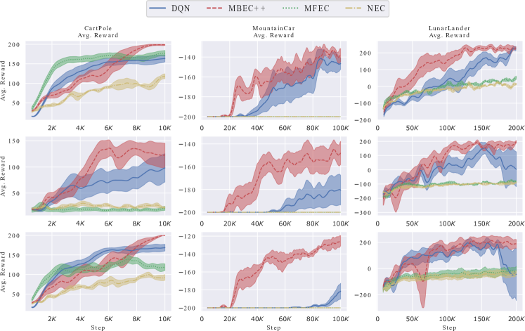
Figure 7: All learning curves for stochastic classical control task. First row: Gaussian noisy reward. Second row: Bernoulli noisy reward. Third row: Noisy transition

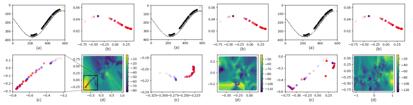
Figure 8: Stochastic Mountain Car. Trajectory space in noisy transition using models trained with TR loss (left), no training (middle) and TP loss (right).

B.3 Stochastic classical control task

Task description

We introduce three ways to make a classical control problem stochastic. First, we add Gaussian noise (mean 0, $\sigma_{re}=0.2$) to the reward that the agent observes. Second, we add Bernoulli-like noise (with a probability $p_{re}=0.2$, the agent receives a reward $-r$ where $r$ is the true reward). Finally, we make the observed transition noisy by letting the agent observe the same state despite taking any action with a probability $p_{tr}=0.5$. The randomness only affects what the agent sees while the environment dynamic is not affected. Three classical control problems are chosen from Open AI’s gym: CartPole-v0, MountainCar-v0 and LunarLander-v2. For each problem, we apply the three stochastic configurations, yielding 9 tasks in total.

Fig. 7 showcases the learning curves of DQN, MBEC++, MFEC and NEC for all 9 tasks. MBEC++ is consistently the leading performer. DQN is often the runner-up, yet usually underperforms our method by a significant margin. Overall, other memory-based methods such as MFEC and NEC perform poorly for these tasks since they are not designed for stochastic environments.

Memory contribution

We determine the episodic and semantic contribution to the final value estimation by counting the number of times their greedy actions equal the final greedy action, dividing by the number of timesteps. Concretely, the episodic and semantic contribution is computed respectively as

$$\frac{\sum_{t=1}^{T}\mathrm{argmax}_{a_{t}}Q_{eps}\left(s_{t},a_{t}\right)==\mathrm{argmax}_{a_{t}}Q\left(s_{t},a_{t}\right)}{T}$$

$$\frac{\sum_{t=1}^{T}\mathrm{argmax}_{a_{t}}Q_{\theta}\left(s_{t},a_{t}\right)==\mathrm{argmax}_{a_{t}}Q\left(s_{t},a_{t}\right)}{T}$$

where $Q_{eps}\left(s_{t},a_{t}\right)=Q_{MBEC}\left(s_{t},a_{t}\right)f_{\beta}\left(s_{t},\overrightarrow{\tau}_{t-1}\right)$, $Q_{\theta}\left(s_{t},a_{t}\right)$ and $Q\left(s_{t},a_{t}\right)$ represent the episodic, semantic and final value estimation, respectively.

Fig. 4 illustrates the running average contribution using a window of 100 timesteps. We note that the contribution of the two does not need to sum up to 1 as both can agree with the same greedy action.

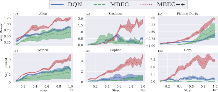
Figure 9: Learning curves of several Atari games.

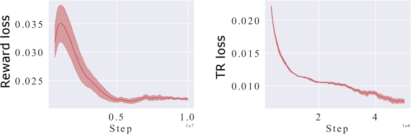
Figure 10: Loss of reward model and TR loss over training iterations for Atari’s Asterix and Gopher, respectively.

Game	Nature DQN	MFEC	NEC	MBEC++
Alien	634.8	1717.7	3460.6	1991.2
Amid	126.8	370.9	811.3	369.0
Assault	1489.5	510.2	599.9	4981.3
Asterix	2989.1	1776.6	2480.4	7724.0
Asteroids	395.3	4706.8	2496.1	1456.2
Atlantis	14210.5	95499.4	51208.0	99270.0
Bank Heist	29.3	163.7	343.3	1126.4
Battlezone	6961.0	19053.6	13345.5	30004.0
Beamrider	3741.7	858.8	749.6	5875.2
Berzerk	484.2	924.2	852.8	759.2
Bowling	35.0	51.8	71.8	80.6
Boxing	31.3	10.7	72.8	95.8
Breakout	36.8	86.2	13.6	372.2
Centipede	4401.4	20608.8	12314.5	8693.8
Chopper Command	827.2	3075.6	5070.3	1694.0
Crazy Climber	66061.6	9892.2	34344.0	107740.0
Defender	2877.90	10052.80	6126.10	690956.0
Demon Attack	5541.9	1081.8	641.4	8066.4
Double Dunk	-19.0	-13.2	1.8	-1.8
Enduro	364.9	0.0	1.4	343.7
Fishing Derby	-81.6	-90.3	-72.2	17.6
Freeway	21.5	0.6	13.5	33.1
Frostbite	339.1	925.1	2747.4	1783.0
Gopher	1111.2	4412.6	2432.3	11386.4
Gravitar	154.7	1011.3	1257.0	428.0
H.E.R.O.	1050.7	14767.7	16265.3	12148.5
Ice Hockey	-4.5	-6.5	-1.6	-1.5
James Bond	165.9	244.7	376.8	898.0
Kangaroo	519.6	2465.7	2489.1	16464.0
Krull	6015.1	4555.2	5179.2	9031.38
Kung Fu Master	17166.1	12906.5	30568.1	37100.0
Montezuma’s Revenge	0.0	76.4	42.1	0.0
Ms. Pac-Man	1657.0	3802.7	4142.8	2687.2
Name This Game	6380.2	4845.1	5532.0	7822.8
Phoenix	5357.0	5334.5	5756.5	15051.8
Pitfall!	0.0	-79.0	0.0	0.0
Pong	-3.2	-20.0	20.4	20.8
Private Eye	100.0	3963.8	162.2	100.0
Q*bert	2372.5	12500.4	7419.2	8686.0
River Raid	3144.9	4195.0	5498.1	10656.4
Road Runner	7285.4	5432.1	12661.4	55284.0
Robot Tank	14.6	7.3	11.1	23.9
Seaquest	618.7	711.6	1015.3	10460.2
Skiing	-19818.0	-15278.9	-26340.7	-10016.0
Solaris	1343.0	8717.5	7201.0	1692.0
Space Invaders	642.2	2027.8	1016.0	1425.6
Stargunner	604.8	14843.9	1171.4	49640.0
Tennis	0.0	-23.7	-1.8	18.8
Time Pilot	1952.0	10751.3	10282.7	6752.0
Tutankham	148.7	86.3	121.6	206.36
Up’n Down	18964.9	22320.8	39823.3	21743.2
Venture	3.8	0.0	0.0	1092.4
Video Pinball	14316.0	90507.7	22842.6	182887.9
Wizard of Wor	401.4	12803.1	8480.7	6252.0
Yars’ Revenge	7614.1	5956.7	21490.5	21889.8
Zaxxon	200.3	6288.1	10082.4	11180.0

Table 3: Scores at 10 million frames.

Trajectory space visualization

We visualize the memory-based value function w.r.t trajectory vectors in Fig. 4 (d). As such, we set the trajectory dimension to $H=2$ and estimate the value for each grid point (step 0.05) using $\mathrm{read}$ operator as

$$V\left(\overrightarrow{\tau}\right)\approx\sum_{i\in\mathcal{N}^{K_{r}}(\overrightarrow{\tau})}\frac{\left\langle\mathcal{M}_{i}^{k},\overrightarrow{\tau}\right\rangle\mathcal{M}_{i}^{v}}{\sum_{j\in\mathcal{N}^{K}(\overrightarrow{\tau})}\left\langle\mathcal{M}_{j}^{k},\overrightarrow{\tau}\right\rangle}$$

To cope with noisy environment, MBEC relies on noise-tolerant trajectory representation. As demonstrated in Fig. 8, even when the state representations are disturbed by not changing to true states, the trajectory representations shaped by the TR loss maintain good approximation and interpolate well the latent location of disturbed trajectories. In contrast, representations generated by random model or model trained with TP loss fail to discover latent location of disturbed trajectories, either collapsing (random model) or shattering (TP loss model).

The failure of TP loss is understandable since it is very hard for predicting the next transition when half of the ground truth is noisy ($p_{tr}=0.5$). On the other hand, TR loss facilitates easier learning wherein the model only needs to reconstruct past observations which are somehow already encoded in the current representation.

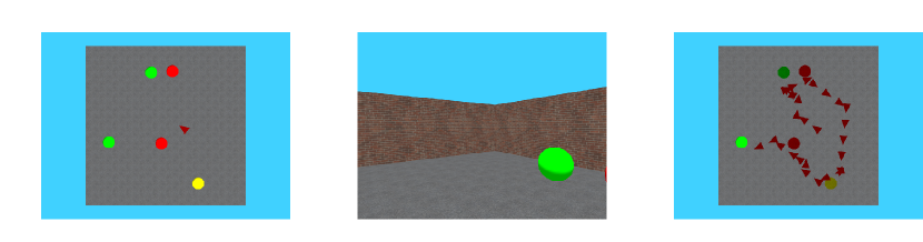
Figure 11: 3D Navigation: picking 5 objects task. Top view map (left) and frontal view-port or the observed state of the agent (middle) and a solution found by MBEC++ (right).

B.4 Atari 2600 task

We use Adam optimizer with a learning rate of $10^{-4}$, batch size of 32 and only train the models within 10 million frames for sample efficiency. Other implementations follows [34] (CNN architecture, exploration rate, 4-frame stacking, reward clipping, etc.). In our implementation, at timestep t, we use frames at t,t-1,t-2,t-3 and still count t as the current frame as well as the current timestep. We tune the hyper-parameters for MBEC++ using the standard validation procedure, resulting in $K=7$, $L=100$ and $N=50,000$.

We also follow the training and validation procedure from [34] using a public DQN implementation. The CNN architecture is a stack of 4 convolutional layers with numbers of filters, kernel sizes and strides of $\left[32,64,64,1024\right]$,$\left[8,4,3,3\right]$ and $\left[4,2,1,1\right]$, respectively. The Atari platform is Open AI’s Atari environments.

In order to understand better the efficiency of MBEC++, we record and compare the learning curves of MBEC++, MBEC and DQN (our implementation using the same training procedure) in Fig. 9. We run the 3 models on 6 games (Alien, Breakout, Fishing Derby, Asterix, Gopher and Hero), and plot the average performance over 5 random seeds. We observe a common pattern for all learning curves, in which the performance gap between MBEC++ and DQN becomes clearer around 5 million steps and gets wider afterwards. We note that MBEC++ demonstrate fast learning curves for some games (e.g., Breakout and Fishing Derby) that other methods (DQN, MFEC or NEC) struggle to learn.

We realize that early stopping of training trajectory model or reward model does not affect the performance much as the quality of trajectory representations and reward prediction is acceptable at about 5 millions steps (see Fig. 10). Early stopping further accelerates the running speed of MBEC++ and also helps stabilize the learning of the Q-Networks.

Table 3 reports the final testing score of MBEC++ and other baselines for all Atari games. We note that we only conducted five runs for the Atari games mentioned in Fig. 9. For the remaining games, our limited compute budget did not allow us to perform multiple runs, and thus, we only ran once. We store the best MBEC++ models based on validation score for each game during training and test them for $100$ episodes. Other baselines’ numbers are reported from [36]. Compared to other baselines, MBEC++ is the winner on the leaderboard for about half of the games.

Notably, our episodic memory is much smaller than that of others. For example, NEC and EMDQN maintain 5 millions slots per action (there are total 18 actions). Meanwhile, our best number of memory slots $N$ is only 50,000.

Model	Alien	Asterix	Breakout	Fishing Derby	Gopher	Hero
Dreamer-v2	2950.1	3100.8	57.0	-13.6	16002.8	13552.9
Our MBEC++	1991.2	7724.0	372.2	17.6	11386.4	12148.5

Table 4: Dreamver-v2 vs MBEC++ on 6 Atari games at 10M frames. We report the best results of the models after three runs.

Model	Alien	Asterix	Breakout	Fishing Derby	Gopher	Hero
SIMPLE♣	378.3 ± 85.5	668.0 ± 294.1	6.1 ± 2.8	-94.5 ± 3.0	510.2 ± 158.4	621.5 ± 1281.3
Our MBEC++	340.5 ± 39.7	810.1 ± 42.4	11.9 ± 2.0	-81.5 ± 2.3	459.2 ± 60.4	1992.8 ± 1171.9

Table 5: SIMPLE vs MBEC++ on 6 Atari games at 400K frames. Mean and std over 5 runs. $\clubsuit$ is from [23].

B.5 3D navigation task

In this task, the agent’s goal is to pick objects randomly located in a big room. There are 5 possible actions (moving directions and object interaction) and the number of objects is customizable. We train MBEC++, DQN and DRQN using the same training procedure and CNN for state encoding as in the Atari task. Except for DQN, other baselines (DRQN and PPO) uses LSTM to encode the state of the environment. We also stack 4 consecutive frames to help the models (especially DQN) cope with the environment’s limited observation. For PPO, we tuned the clipping threshold {0.2, 0.5, 0.8} and reported the best result (0.2).

Fig. 11 illustrates one sample of the environment map and a solution found by MBEC++. The best hyper-parameters for MBEC++ are $K=15$, $L=20$ and $N=10000$.

B.6 Ablation study

Classical control

We tune MBEC++ with Noisy Transition Mountain Car problem using range $K\in\left\{1,5,15\right\}$, $L=\left\{1,10,50\right\}$, $N=\left\{500,3000,30000\right\}$. We use the best found hyper-parameters ($K=15$, $L=10$, $N=3000$) for all 9 problems. The learning curves of MBEC++ in Noisy Transition Mountain Car are visualized in Fig. 5 (the first 3 plots).

We also conduct an ablation study on MBEC++: (i) without TR loss, (ii) with TP loss instead (iii), without multiple write ($K_{w}=1$) and (iv) without memory refining. The result demonstrates that ablating any components reduces the performance of MBEC++ significantly (see Fig. 5 (the final plot)).

Dynamic consolidation

We compare our dynamic consolidation with traditional fixed combinations in both simple and complex environments. Fixed combination baselines use fixed $\beta$ in Eq. 7, resulting in

$$Q\left(s_{t},a_{t}\right)=Q_{MBEC}\left(s_{t},a_{t}\right)\beta+Q_{\theta}\left(s_{t},a_{t}\right)$$

In CartPole (Gaussian noisy reward), all fixed combinations achieve moderate results, yet fails to solve the task after 10,000 training steps. Dynamic consolidation learning to generate dynamic $\beta$, in contrast, completely solves the task (see Fig. 13 (a)).

In Atari game’s Riverrraid–a more complex environment, the performance gap between dynamic $\beta$ and fixed $\beta$ becomes clearer. Average reward of dynamic consolidation reaches nearly 7,000 while the best fixed combination’s ($\beta=0.1$) is less than 3,000 (see Fig. 13 (b)).

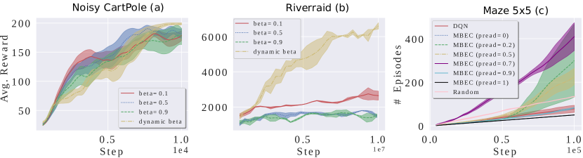
Figure 13: Ablation studies on dynamic consolidation (a,b) and $p_{read}$ (c). All curves are reported with mean and std. over 5 runs.

Tuning $p_{read}$

Besides modified modes introduced in the main manuscript, we investigate MBEC with different $p_{read}$ and DQN in a bigger maze ($5\times 5$) for the original setting. As shown in Fig. 13 (c), many MBEC variants successfully learn the task, significantly better in the number of completed episodes compared to random and DQN agents. We find that when $p_{read}=1$ (only average reading), the performance of MBEC is negatively affected, which indicates that the role of max reading is important. Similar situation is found for for $p_{read}=0$ (only max reading). Among all variants, $p_{read}=0.7$ shows stable and fastest learning. Hence, we set $p_{read}=0.7$ for all other experiments in this paper.

References

- [1] Jose A Arjona-Medina, Michael Gillhofer, Michael Widrich, Thomas Unterthiner, Johannes Brandstetter, and Sepp Hochreiter. Rudder: Return decomposition for delayed rewards. In Advances in Neural Information Processing Systems, pages 13566–13577, 2019.
- [2] Alan D Baddeley and Graham Hitch. Working memory. In Psychology of learning and motivation, volume 8, pages 47–89. Elsevier, 1974.
- [3] Marc G Bellemare, Yavar Naddaf, Joel Veness, and Michael Bowling. The arcade learning environment: An evaluation platform for general agents. Journal of Artificial Intelligence Research, 47:253–279, 2013.
- [4] Charles Blundell, Benigno Uria, Alexander Pritzel, Yazhe Li, Avraham Ruderman, Joel Z Leibo, Jack Rae, Daan Wierstra, and Demis Hassabis. Model-free episodic control. arXiv preprint arXiv:1606.04460, 2016.
- [5] Maxime Chevalier-Boisvert. gym-miniworld environment for openai gym. https://github.com/maximecb/gym-miniworld, 2018.
- [6] Yadin Dudai and Mary Carruthers. The janus face of mnemosyne. Nature, 434(7033):567–567, 2005.
- [7] Simon Farrell. Temporal clustering and sequencing in short-term memory and episodic memory. Psychological review, 119(2):223, 2012.
- [8] Meire Fortunato, Melissa Tan, Ryan Faulkner, Steven Hansen, Adrià Puigdomènech Badia, Gavin Buttimore, Charlie Deck, Joel Z Leibo, and Charles Blundell. Generalization of reinforcement learners with working and episodic memory. In NeurIPS, 2019.
- [9] Samuel J Gershman and Nathaniel D Daw. Reinforcement learning and episodic memory in humans and animals: an integrative framework. Annual review of psychology, 68:101–128, 2017.
- [10] Alex Graves, Greg Wayne, and Ivo Danihelka. Neural turing machines. arXiv preprint arXiv:1410.5401, 2014.
- [11] Alex Graves, Greg Wayne, Malcolm Reynolds, Tim Harley, Ivo Danihelka, Agnieszka Grabska-Barwińska, Sergio Gómez Colmenarejo, Edward Grefenstette, Tiago Ramalho, John Agapiou, et al. Hybrid computing using a neural network with dynamic external memory. Nature, 538(7626):471–476, 2016.
- [12] Joseph F Grcar. A matrix lower bound. Linear algebra and its applications, 433(1):203–220, 2010.
- [13] David Ha and Jürgen Schmidhuber. Recurrent world models facilitate policy evolution. In Advances in neural information processing systems, pages 2450–2462, 2018.
- [14] Danijar Hafner, Timothy Lillicrap, Ian Fischer, Ruben Villegas, David Ha, Honglak Lee, and James Davidson. Learning latent dynamics for planning from pixels. In International Conference on Machine Learning, pages 2555–2565. PMLR, 2019.
- [15] Danijar Hafner, Timothy P Lillicrap, Mohammad Norouzi, and Jimmy Ba. Mastering atari with discrete world models. In International Conference on Learning Representations, 2020.
- [16] Steven Hansen, Alexander Pritzel, Pablo Sprechmann, André Barreto, and Charles Blundell. Fast deep reinforcement learning using online adjustments from the past. In Advances in Neural Information Processing Systems, pages 10567–10577, 2018.
- [17] Matthew Hausknecht and Peter Stone. Deep recurrent q-learning for partially observable mdps. arXiv preprint arXiv:1507.06527, 2015.
- [18] Frank S He, Yang Liu, Alexander G Schwing, and Jian Peng. Learning to play in a day: Faster deep reinforcement learning by optimality tightening. In 5th International Conference on Learning Representations, ICLR 2017, 2019.
- [19] Sepp Hochreiter and Jürgen Schmidhuber. Long short-term memory. Neural computation, 9(8):1735–1780, 1997.
- [20] Hao Hu, Jianing Ye, Zhizhou Ren, Guangxiang Zhu, and Chongjie Zhang. Generalizable episodic memory for deep reinforcement learning. arXiv preprint arXiv:2103.06469, 2021.
- [21] Chia-Chun Hung, Timothy Lillicrap, Josh Abramson, Yan Wu, Mehdi Mirza, Federico Carnevale, Arun Ahuja, and Greg Wayne. Optimizing agent behavior over long time scales by transporting value. Nature communications, 10(1):1–12, 2019.
- [22] Tommi Jaakkola, Michael I Jordan, and Satinder P Singh. On the convergence of stochastic iterative dynamic programming algorithms. Neural computation, 6(6):1185–1201, 1994.
- [23] Lukasz Kaiser, Mohammad Babaeizadeh, Piotr Milos, Blazej Osinski, Roy H Campbell, Konrad Czechowski, Dumitru Erhan, Chelsea Finn, Piotr Kozakowski, Sergey Levine, et al. Model-based reinforcement learning for atari. arXiv preprint arXiv:1903.00374, 2019.
- [24] Dharshan Kumaran, Demis Hassabis, and James L McClelland. What learning systems do intelligent agents need? complementary learning systems theory updated. Trends in cognitive sciences, 20(7):512–534, 2016.
- [25] Hung Le, Truyen Tran, and Svetha Venkatesh. Learning to remember more with less memorization. arXiv preprint arXiv:1901.01347, 2019.
- [26] Hung Le, Truyen Tran, and Svetha Venkatesh. Self-attentive associative memory. In Proceedings of the 37th International Conference on Machine Learning, volume 119 of Proceedings of Machine Learning Research, pages 5682–5691, Virtual, 13–18 Jul 2020. PMLR.
- [27] Hung Le and Svetha Venkatesh. Neurocoder: Learning general-purpose computation using stored neural programs. arXiv preprint arXiv:2009.11443, 2020.
- [28] Su Young Lee, Choi Sungik, and Sae-Young Chung. Sample-efficient deep reinforcement learning via episodic backward update. In Advances in Neural Information Processing Systems, pages 2112–2121, 2019.
- [29] Máté Lengyel and Peter Dayan. Hippocampal contributions to control: the third way. In Advances in neural information processing systems, pages 889–896, 2008.
- [30] Zichuan Lin, Tianqi Zhao, Guangwen Yang, and Lintao Zhang. Episodic memory deep q-networks. arXiv preprint arXiv:1805.07603, 2018.
- [31] James L McClelland, Bruce L McNaughton, and Randall C O’Reilly. Why there are complementary learning systems in the hippocampus and neocortex: insights from the successes and failures of connectionist models of learning and memory. Psychological review, 102(3):419, 1995.
- [32] Francisco S Melo. Convergence of q-learning: A simple proof. Institute Of Systems and Robotics, Tech. Rep, pages 1–4, 2001.
- [33] Volodymyr Mnih, Adria Puigdomenech Badia, Mehdi Mirza, Alex Graves, Timothy Lillicrap, Tim Harley, David Silver, and Koray Kavukcuoglu. Asynchronous methods for deep reinforcement learning. In International conference on machine learning, pages 1928–1937, 2016.
- [34] Volodymyr Mnih, Koray Kavukcuoglu, David Silver, Andrei A Rusu, Joel Veness, Marc G Bellemare, Alex Graves, Martin Riedmiller, Andreas K Fidjeland, Georg Ostrovski, et al. Human-level control through deep reinforcement learning. nature, 518(7540):529–533, 2015.
- [35] Daichi Nishio and Satoshi Yamane. Faster deep q-learning using neural episodic control. In 2018 IEEE 42nd Annual Computer Software and Applications Conference (COMPSAC), volume 1, pages 486–491. IEEE, 2018.
- [36] Alexander Pritzel, Benigno Uria, Sriram Srinivasan, Adria Puigdomenech Badia, Oriol Vinyals, Demis Hassabis, Daan Wierstra, and Charles Blundell. Neural episodic control. In Proceedings of the 34th International Conference on Machine Learning-Volume 70, pages 2827–2836. JMLR. org, 2017.
- [37] Tom Schaul, John Quan, Ioannis Antonoglou, and David Silver. Prioritized experience replay. arXiv preprint arXiv:1511.05952, 2015.
- [38] John Schulman, Filip Wolski, Prafulla Dhariwal, Alec Radford, and Oleg Klimov. Proximal policy optimization algorithms. arXiv preprint arXiv:1707.06347, 2017.
- [39] Richard S Sutton. Dyna, an integrated architecture for learning, planning, and reacting. ACM Sigart Bulletin, 2(4):160–163, 1991.
- [40] Richard S Sutton and Andrew G Barto. Reinforcement learning: An introduction. MIT press, 2018.
- [41] Endel Tulving. Episodic memory: From mind to brain. Annual review of psychology, 53(1):1–25, 2002.
- [42] Endel Tulving et al. Episodic and semantic memory. Organization of memory, 1:381–403, 1972.
- [43] Christopher JCH Watkins and Peter Dayan. Q-learning. Machine learning, 8(3-4):279–292, 1992.
- [44] Greg Wayne, Chia-Chun Hung, David Amos, Mehdi Mirza, Arun Ahuja, Agnieszka Grabska-Barwinska, Jack Rae, Piotr Mirowski, Joel Z Leibo, Adam Santoro, et al. Unsupervised predictive memory in a goal-directed agent. arXiv preprint arXiv:1803.10760, 2018.
- [45] Vinicius Zambaldi, David Raposo, Adam Santoro, Victor Bapst, Yujia Li, Igor Babuschkin, Karl Tuyls, David Reichert, Timothy Lillicrap, Edward Lockhart, et al. Deep reinforcement learning with relational inductive biases. In International Conference on Learning Representations, 2018.
- [46] Guangxiang Zhu, Zichuan Lin, Guangwen Yang, and Chongjie Zhang. Episodic reinforcement learning with associative memory. In International Conference on Learning Representations, 2019.