Linking Across Data Granularity: Fitting Multivariate Hawkes Processes to Partially Interval-Censored Data

Abstract

The multivariate Hawkes process (MHP) is widely used for analyzing data streams that interact with each other, where events generate new events within their own dimension (via self-excitation) or across different dimensions (via cross-excitation). However, in certain applications, the timestamps of individual events in some dimensions are unobservable, and only event counts within intervals are known, referred to as partially interval-censored data. The MHP is unsuitable for handling such data since its estimation requires event timestamps. In this study, we introduce the Partial Mean Behavior Poisson (PMBP) process, a novel point process which shares parameter equivalence with the MHP and can effectively model both timestamped and interval-censored data. We demonstrate the capabilities of the PMBP process using synthetic and real-world datasets. Firstly, we illustrate that the PMBP process can approximate MHP parameters and recover the spectral radius using synthetic event histories. Next, we assess the performance of the PMBP process in predicting YouTube popularity and find that it surpasses state-of-the-art methods. Lastly, we leverage the PMBP process to gain qualitative insights from a dataset comprising daily COVID-19 case counts from multiple countries and COVID-19-related news articles. By clustering the PMBP-modeled countries, we unveil hidden interaction patterns between occurrences of COVID-19 cases and news reporting.

I Introduction

The Hawkes process, introduced by [1], is a temporal point process that exhibits the self-exciting property, i.e., the occurrence of one event increases the likelihood of future events. The Hawkes process is widely applied in both the physical and social sciences. For example, earthquakes are known to be temporally clustered: the mainshock is often the first in a sequence of subsequent aftershocks. In online social media, tweets by influential users typically induce cascades of retweets as the message diffuses over the social network [2]. The multivariate Hawkes process (MHP) [1] extends the univariate process by allowing events to occur in multiple parallel timelines — dubbed as dimensions. These dimensions interact via cross-excitation, i.e., events in one dimension can spawn events in the other dimensions. Fig. 1 schematically exemplifies the interaction between two social media platforms: YouTube and Twitter. An initial tweet (denoted as A on the figure) spawns a retweet (B) via self-excitation and a view (C) via cross-excitation. The cross-excitation goes both ways: the view C generates the tweet D.

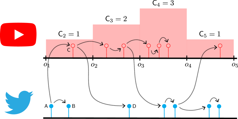
Figure 1: Example of multi-platform interaction between view events on YouTube (red lollipops) and tweets on Twitter (blue lollipops). The data is partially interval-censored, as YouTube does not expose individual views, but only the view counts $\mathsf{C}_{i}$’s over the predefined intervals $[o_{i},o_{i+1})$ (shown as red rectangles). The dashed lines show the latent branching structure between views and tweets. The red lollipops are also dashed and empty, indicating that YouTube views are not observed.

Given the event timestamps, we can fit the parameters of the Hawkes process using maximum likelihood estimation (MLE). However, in many practical applications, the event times are not observed, and only counts over predefined time partitions are available. We denote such data as interval-censored. For multivariate data, we denote the case when all dimensions are interval-censored as completely interval-censored. If only a subset of dimensions is interval-censored, we have partially interval-censored data.

One reason for interval-censoring is data availability — for epidemic data [3], we usually observe the aggregated daily counts of reported cases instead of detailed case information. Another reason is space limitations — for network traffic data [4], storing high-resolution event logs is impractical; they are stored as summaries over bins instead. A third reason is data privacy. This is the case for YouTube, as shown in the upper half of Fig. 1, where the individual views are interval-censored, and we only observe aggregated daily counts.

This paper tackles three open questions about using the MHP with partially interval-censored data. The first question relates to fitting the process to both event time and interval-censored data. When the data is presented as event times, the MHP can be fitted using MLE [5]. However, if the data is partially or completely interval-censored, MLE cannot fit the MHP process parameters because it lacks the independent increments property [6]. Given interval-censored counts, one could approach fitting the Hawkes process naïvely by sampling event times uniformly over the intervals [7]. However, this quickly hits scalability issues for high interval-censored counts. For instance, the Youtube videos in our real-world dataset often have millions of views per day. For completely interval-censored univariate data, [6] proposed the Mean Behavior Poisson (MBP) — an inhomogeneous Poisson process that approximates the mean behavior of the Hawkes process — to estimate the parameters of a corresponding Hawkes process. However, a model and fitting scheme remained elusive for the partially interval-censored data. The question is, can we devise a method to fit the MHP in the partially interval-censored setting? What are the limits to MHP parameter recovery in the partially interval-censored setting?

The second question relates to modeling and forecasting online popularity across social media platform boundaries. Online popularity has been extensively studied within the realm of a single social media platform — see Twitter [8, 9, 10, 11], YouTube [12, 13], Reddit [14] — and the self-exciting point processes are the tool of choice for modeling. However, content is often shared across multiple interacting platforms — such as YouTube and Twitter — and we need to account for cross-excitation using multivariate processes. However, YouTube only exposes view data as interval-censored, rendering it impossible to use the classical MHP. The Hawkes Intensity process (HIP) [13] proposes a workaround and treats the tweet and share counts as external stimuli for views. Its shortcoming is that it cannot model the cross-excitation from views to tweets and shares. The question is, can we improve performance in the YouTube popularity prediction task by modeling the views, tweets, and shares through fitting on partially interval-censored data?

The third question concerns analyzing interaction patterns across the online and offline environments, enabling us, for example, to determine whether online activity preempts or reacts to events that happen offline. Previous work has demonstrated the complex link between news and infectious disease outbreaks, notably the 2009 A/H1N1 outbreak in the Shaanxi province in China [15], the 2010 cholera outbreak in Haiti [16], and the early spread of COVID in 2020 in various provinces in China [17]. The association between media and case counts has typically been investigated by examining the cross-correlation of the news counts and case counts as paired time series and demonstrating that significant correlations exist when temporal lags are applied. [15, 17] show correlations between news and cases for both positive and negative lags, suggesting that news both had an impact and had been impacted by reported disease counts. [16] show that news typically lags behind cases; they also showcase how news counts can be used as a proxy for estimating crucial disease measures such as the basic reproduction number $R_{0}$. This highlights that the connection between news and cases is particularly relevant given that news counts can be retrieved in near real-time; in contrast, official case counts reporting is often lagging. In most previous work, uncovering time-series cross-correlation is the focus, without building explanatory models to produce nuanced views of the interactions through interpretable parameters. The question is, can we apply MHP on partially interval-censored data to uncover country-level differences in the interplay between recorded daily case counts of COVID-19 and the publication of COVID-19-related news articles?

We address these three questions by introducing the Partial Mean Behavior Poisson (PMBP) process, a novel multivariate temporal point process that operates on partially interval-censored data. We answer the first question in Section II-B, where we detail the PMBP process. The event intensity of PMBP on the interval-censored dimensions is determined by the expected Hawkes intensity, considering the stochastic history of those dimensions conditioned on the event time dimensions. On the event time dimensions, the intensity of PMBP corresponds to that of the respective Hawkes process. This construction allows us to fit the PMBP process to partially interval-censored data and estimate the parameters of the multivariate Hawkes process through parameter equivalence.

We address the second question in Section IV by using PMBP to predict the popularity of YouTube videos on both YouTube and Twitter. We demonstrate that PMBP consistently outperforms the current state-of-the-art HIP method [13], provides quantification of prediction uncertainty and extends predictions to all dimensions — unlike HIP, which can only predict the views’ dimension.

We address the third question in Section V by utilizing PMBP to investigate the relationship between COVID-19 case incidence and news coverage. We fit country-specific PMBP processes for 11 countries using a dataset consisting of reported COVID-19 cases (with interval-censored data) and the publication dates of COVID-19-related news articles during the early stage of the outbreak. We identify three distinct groupings by clustering countries using the fitted PMBP parameters. In the first group (UK, Spain, Germany, and Brazil), we observe preemptive news coverage, where an increase in news leads to a rise in cases. The second group (China and France) exhibits reactionary news coverage, with news lagging behind the cases. No significant interaction between news and cases is found in the third group (US, Italy, Sweden, India, and the Philippines).

I-A Related Work

A significant portion of recent literature on the Hawkes process, and on point processes in general, deals with estimation from partially observed data. This problem is nontrivial as standard MLE techniques require the complete dataset.

It was shown in [18] that a sequence of (integer-valued autoregressive time series) INAR($\infty$)-based family of point processes converges to the Hawkes process. Under this convergence, they concluded that the INAR($\infty$) is the discrete-time version of the Hawkes process. In a follow-up, [19] presented an alternative procedure to MLE, which fits the associated bin-count sequences to the INAR($p$) process. As the bin size goes to zero and the order $p$ of the process goes to $\infty$, the INAR sequence converges to the Hawkes process and the parameter estimates converge to the Hawkes parameters. However, though fitting is performed on count data, convergence only actually occurs for small bin size.

A spectral approach to fitting the Hawkes process given interval-censored data for arbitrary bin size is presented in [20], solving the issue in [19]. Their proposed method is based on minimizing the log-spectral likelihood of the bin-count sequence instead of the usual log-likelihood of the Hawkes process. They showed that optimization converges to the Hawkes parameters under certain assumptions on the kernel.

Another alternative approach is presented in [4], which introduced a Monte Carlo Expectation Maximization (MC-EM) algorithm that uses sampling to obtain proposals for the hidden event times. They showed that their approach recovers parameters more reliably than the INAR(p) estimates from [19] in synthetic experiments. They further extended their approach to the multivariate case in [21]. Reliance on sampling makes this approach more computationally expensive than the others.

II Model

II-A Background

A temporal point process can be specified by its conditional intensity function. Let $\textbf{{N}}(t)$ represent the number of events that occurred up until time $t$ and $\mathcal{H}^{j}_{t^{-}}$ be the set of all events that occur in dimension $j$ up until $t$, for $j\in 1\cdots d$. The conditional intensity function $\boldsymbol{\lambda^{\star}}(t)\vcentcolon=\boldsymbol{\lambda}\left(t|\bigcup_{j=1}^{d}\mathcal{H}^{j}_{t^{-}}\right)$ is defined as

$$\lambda^{j}\left(t\Bigg{|}\bigcup_{j=1}^{d}\mathcal{H}^{j}_{t^{-}}\right)=\lim_{h\rightarrow 0^{+}}\frac{1}{h}\mathbb{P}\left\{N^{j}(t+h)-N^{j}=1\Bigg{|}\bigcup_{j=1}^{d}\mathcal{H}^{j}_{t^{-}}\right\},$$

which gives the instantaneous probability of a dimension $j$ event occurring in the increment $[t,t+dt)$, conditioned on all events that happen before $t$.

Hawkes Process: The univariate Hawkes process is a type of temporal point process that models a sequence of events on a single dimension exhibiting a self-exciting behavior. Given $d$ types of events, the corresponding $d$-dimensional multivariate Hawkes process (MHP) is a point process where each dimension tracks the dynamics of each event type. In addition to being self-exciting, the MHP is cross-exciting among event types, i.e., an event occurring in one type of event increases the probability of any type of event occurring in the near future. The conditional intensity of the $d$-dimensional Hawkes process is given by

$$\boldsymbol{\lambda^{\star}}(t)\vcentcolon=\boldsymbol{\mu}(t)+\sum_{j=1}^{d}\sum_{t_{k}^{j}<t}\boldsymbol{\varphi}^{j}(t-t^{j}_{k}),$$ (1)

where $\boldsymbol{\mu}(t)$ is called the background intensity controlling the arrival of external events into the system. The matrix $\boldsymbol{\varphi}(t)$ is called the Hawkes kernel, a $d\times d$ matrix of functions that characterizes the self- and cross-excitation across the event types representing the $d$ dimensions. Let $\boldsymbol{\varphi}^{j}(t)$ represent the $j^{th}$ column of the Hawkes kernel. The diagonal entries $\varphi^{jj}(t)$ and off-diagonal entries $\varphi^{ij}(t)$, $i\neq j$, represent the self- and cross-exciting components of the Hawkes kernel, respectively.

The Hawkes kernel is often specified in a parametric form to facilitate simple interpretability. Let $D$ denote the index set $\{1,\ldots,d\}$. If we assume $\varphi^{ij}(t)=\alpha^{ij}f^{ij}(t)$, $\alpha^{ij}\geq 0$, $f^{ij}(t)\geq 0$, and $\int^{\infty}_{0}f^{ij}(t)\mathrm{d}t=1$ for $(i,j)\in D\times D$. We call $\alpha^{ij}$ the branching factor from $j$ to $i$ and the matrix $\boldsymbol{\alpha}=(\alpha^{ij})\in(\mathbb{R}^{+})^{d\times d}$ the branching matrix. The branching factor $\alpha^{ij}$ gives the expected number of direct offsprings in dimension $j$ spawned by a parent of dimension $i$. For the function $f^{ij}(t)$, we consider the commonly used exponential kernel $\varphi^{ij}(t)=\alpha^{ij}\theta^{ij}\exp(-\theta^{ij}t)$, where $\theta^{ij}$ controls the rate of influence decay from $j$ to $i$. More prerequisite details on the MHP are provided in Sec. 1.1 of the SI [22].

Mean Behavior Poisson Process: Consider a univariate Hawkes process with conditional intensity $\lambda(t|\mathcal{H}_{t^{-}})$. The Mean Behavior Poisson (MBP) process introduced by [6] is the inhomogeneous Poisson process with conditional intensity $\xi(t)$ given by

$$\xi(t)\vcentcolon={\mathbb{E}_{\mathcal{H}_{t^{-}}}}\left[\lambda(t|\mathcal{H}_{t^{-}})\right]=\mu(t)+(\varphi*\xi)(t),$$ (2)

where $*$ denotes convolution. The MBP intensity can be viewed as the average Hawkes process intensity over its set of realizations.

[6] showed that $\mu(t)\Mapsto\xi(t)$ in LABEL:{eq:mbp_intensity_convolution} defines a linear time-invariant (LTI) system [23], meaning that it obeys linearity ($\mu_{1}(t)\Mapsto\xi_{1}(t)$ and $\mu_{2}(t)\Mapsto\xi_{2}(t)$ imply that $a\mu_{1}(t)+b\mu_{2}(t)\Mapsto a\xi_{1}(t)+b\xi_{2}(t)$ for $a,b\in\mathbb{R}$) and time invariance ($\mu(t)\Mapsto\xi(t)$ implies that $\mu(t-t_{0})\Mapsto\xi(t-t_{0})$ for $t_{0}>0$.) As an LTI system, the response $\xi(t)$ to the input $\mu(t)$ can be obtained by solving for the response of the system to the Dirac impulse $\delta(t)$, derived in [6] to be

$$\xi(t)=\left(\delta(t)+\sum_{n=1}^{\infty}\varphi^{\otimes n}(t)\right)*\mu(t),$$ (3)

where $\otimes n$ corresponds to $n$-time convolution.

Since the MBP process is a Poisson process, its increments are independent, which allows the likelihood function to be expressed as a sum of the likelihood of disjoint Poisson distributions. This enables the MBP process to be fitted in interval-censored settings via MLE. More prerequisite details are provided in Sec. 1.2 of the SI [22].

Hawkes Intensity Process: The Hawkes intensity process (HIP), introduced in [13], is a temporal point process that can be fit to interval-censored data. It was used primarily for the task of YouTube popularity prediction, where the views on a particular YouTube video are interval-censored, and external shares and tweets that mention the video act as the exogenous intensity $\mu(t)$.

Given a partition $\mathcal{P}[0,T)=\bigcup_{k=1}^{m}[o_{k-1},o_{k})$, where $o_{0}=0$ and $o_{m}=T$, and the associated view counts $\{\mathsf{C}_{k}\}_{k=1}^{m}$, the HIP model is fitted by finding the parameter set $\boldsymbol{\Theta}$ that minimizes the sum of squares error $\sum_{k=1}^{m}\left(\mathsf{C}_{k}-\hat{\xi}[o_{k};\boldsymbol{\Theta}]\right)^{2}$ where $\hat{\xi}[\cdot]$ is given by

$$\hat{\xi}[o_{k};\boldsymbol{\Theta}]=\mu[o_{k}]+\sum_{s=0}^{k-1}\varphi(o_{k}-o_{s};\boldsymbol{\Theta})\cdot\hat{\xi}[o_{s};\boldsymbol{\Theta}].$$

The use of brackets emphasizes that the quantities are discretized over a partition of time. It was shown in [6] that HIP is a discretized approximation of the MBP process.

II-B Partial Mean Behavior Poisson Process

We define the Partial Mean Behavior Poisson process $\textsc{PMBP}(d,e)$ with intensity $\boldsymbol{\xi}_{E}(t)$ as follows.

Definition 1.

Consider a $d$-dimensional Hawkes process with conditional intensity $\boldsymbol{\lambda}^{\star}(t)$ as defined in Eq. 1. Given a nonnegative integer $e\leq d$ and the index sets $D\vcentcolon=\{1,\ldots,d\}$, $E\vcentcolon=\{1,\ldots,e\}$ and $E^{c}\vcentcolon=\{e+1,\ldots,d\}$, the Partial Mean Behavior Poisson process $\textsc{PMBP}(d,e)$ is the temporal point process whose conditional intensity $\boldsymbol{\xi}_{E}(t)$ is the expectation of $\boldsymbol{\lambda^{\star}}(t)$ conditioned on the set of event histories $\bigcup_{j\in E^{c}}\mathcal{H}^{j}_{t^{-}}$ in the $E^{c}$ dimensions and averaged over the set of event histories $\bigcup_{j\in E}\mathcal{H}^{j}_{t^{-}}$ in the $E$ dimensions. That is,

$$\boldsymbol{\xi}_{E}(t)\vcentcolon=\boldsymbol{\xi}\left(t\Big{|}\bigcup_{j\in E^{c}}\mathcal{H}^{j}_{t^{-}}\right)={\mathbb{E}_{\bigcup_{j\in E}\mathcal{H}^{j}_{t^{-}}}}\left[\boldsymbol{\lambda^{\star}}(t)\Big{|}\bigcup_{j\in E^{c}}\mathcal{H}^{j}_{t^{-}}\right].$$ (4)

The $\textsc{PMBP}(d,e)$ process can be viewed as a collection of $d$ processes where the dynamics in the $E$ dimensions follow an $e$-dimensional inhomogeneous Poisson process and the $E^{c}$ dimensions are governed by a ($d-e$)-dimensional Hawkes process. In practice, $E$ would be chosen to be the set of dimensions where event times are inaccessible and only interval-censored event counts can be obtained, while $E^{c}$ would be the dimensions with event time information. In Fig. 1 for instance $E$ would be YouTube views and $E^{c}$ the set of tweets.

It is clear from Eq. 4 that $\textsc{PMBP}(d,e)$ process generalizes both the MHP (by setting $e=0$) and the MBP process (by setting $e=d$).

Convolutional Formula: Consider the kernel $\boldsymbol{\varphi}(t)=\left[\begin{array}[]{cccccc}\boldsymbol{\varphi}^{1}(t)&\ldots&\boldsymbol{\varphi}^{e}(t)&\boldsymbol{\varphi}^{e+1}(t)&\ldots&\boldsymbol{\varphi}^{d}(t)\end{array}\right]$, setting $\boldsymbol{\varphi}^{j}(t)$ to be the $j^{th}$ column of $\boldsymbol{\varphi}(t)$.

Similarly, let $\boldsymbol{\varphi}_{E}(t)=\left[\begin{array}[]{cccccc}\boldsymbol{\varphi}^{1}(t)&\ldots&\boldsymbol{\varphi}^{e}(t)&0&\ldots&0\end{array}\right]$ and $\boldsymbol{\varphi}_{E^{c}}(t)=\left[\begin{array}[]{cccccc}0&\ldots&0&\boldsymbol{\varphi}^{e+1}(t)&\ldots&\boldsymbol{\varphi}^{d}(t)\\ \end{array}\right]$.

Similar to MBP, $\boldsymbol{\xi}_{E}(t)$ can be expressed as the response of an LTI system, which allows us to express $\boldsymbol{\xi}_{E}(t)$ as a convolution with the Dirac impulse $\boldsymbol{\delta}(t)$.

Theorem 2.

Given the Hawkes process with intensity Eq. 1 and kernel parameters satisfying $\lim_{n\rightarrow\infty}\boldsymbol{\varphi}_{E}^{\otimes n}(t)=0$, the conditional intensity of the $\textsc{PMBP}(d,e)$ process is

$$\boldsymbol{\xi}_{E}(t)=\left[\boldsymbol{\delta}(t)+\sum^{\infty}_{n=1}\boldsymbol{\varphi}_{E}^{\otimes n}(t)\right]*\left[\boldsymbol{\mu}(t)+\sum_{j\in E^{c}}\sum_{t^{j}_{k}<t}\boldsymbol{\varphi}^{j}_{E^{c}}(t-t^{j}_{k})\right],$$ (5)

In general, $\boldsymbol{\xi}_{E}(t)$ does not admit a closed form solution because of the complexity of the infinite convolution sum of $\boldsymbol{\varphi}_{E}(t)$ (an interpretation of which is provided in Sec. 2 of the SI [22]). However, in the special case of $\textsc{PMBP}(2,1)$ with the exponential kernel, a closed-form solution for $\boldsymbol{\xi}_{E}(t)$ exists, as proven in Sec. 3 of the SI.

Regularity Conditions: Imposing regularity conditions on the model parameters ensure process subcriticality, i.e. the expected number of direct and indirect offspring spawned by a single parent is finite. For instance, an MHP is subcritical if the spectral radius (i.e. magnitude of the largest eigenvalue) of the branching matrix is less than one, i.e. $\rho(\boldsymbol{\alpha})<1$ [24]. Here we introduce the regularity conditions applicable for the $\textsc{PMBP}(d,e)$ process.

Consider the following submatrices of the branching matrix $\boldsymbol{\alpha}$:

$$\boldsymbol{\alpha}^{EE} =(\alpha^{ij})_{(i,j)\in E\times E}, \boldsymbol{\alpha}^{EE^{c}} =(\alpha^{ij})_{(i,j)\in E\times E^{c}},$$

$$\boldsymbol{\alpha}^{E^{c}E} =(\alpha^{ij})_{(i,j)\in E^{c}\times E}, \boldsymbol{\alpha}^{E^{c}E^{c}} =(\alpha^{ij})_{(i,j)\in E^{c}\times E^{c}}.$$

The following are three conditions which ensure subcriticality of $\textsc{PMBP}(d,e)$.

Theorem 3.

The $\textsc{PMBP}(d,e)$ process with branching matrix $\boldsymbol{\alpha}$ is subcritical if the following conditions hold.

$$\rho(\boldsymbol{\alpha}^{EE})<1\text{, }\quad\rho(\boldsymbol{\alpha}^{E^{c}E^{c}})<1\text{, }\quad\rho(\boldsymbol{\alpha}^{E^{c}E}(\mathbf{I}-\boldsymbol{\alpha}^{EE})^{-1}\boldsymbol{\alpha}^{EE^{c}})<1.$$

We note that the regularity conditions for $\textsc{PMBP}(d,e)$ in Theorem 3 cover the MHP and the MBP as special cases.

Proofs of Theorem 2 and Theorem 3 and a discussion on the nonlinear extension of the PMBP process are provided in Sec. 4 of the SI [22].

II-C Inference

We now consider the problem of estimating the PMBP parameter set $\boldsymbol{\Theta}$ given a $d-$dimensional dataset consisting of a mix of interval-censored data on a subset of dimensions and exact event sequences on the other dimensions.

Consider a $d-$dimensional dataset over the time interval $[0,T)$ such that observations in the first $q$ dimensions are interval-censored, and in the last $d-q$ dimensions, we observe event times. Formally, let $Q\vcentcolon=\{1,\ldots,q\}$ and $Q^{c}\vcentcolon=\{q+1,\ldots,d\}$. For $j\in Q$, we associate a set of observation points $o_{0}^{j}<o_{1}^{j}<\ldots<o_{n^{j}}^{j}$ such that for $o_{k}^{j}$ where $k\geq 1$, we observe the volume $\mathsf{C}^{j}_{k}$ of dimension $j$ events that occurred during the interval $[o_{k-1}^{j},o_{k}^{j})$. Meanwhile, for $j\in Q^{c}$, we observe event sequences $\mathcal{H}_{T^{-}}^{j}=\{t^{j}_{1}<t^{j}_{2}<\ldots<t^{j}_{n^{j}}\}$.

We use MLE to fit the parameters of a $\textsc{PMBP}(d,e)$ process to the above-defined data using the log-likelihood function derived below. The proof is available in Sec. 5 of the SI [22].

Theorem 4.

Given event times $\bigcup_{j\in Q^{c}}\mathcal{H}_{T^{-}}^{j}$, event volumes $\bigcup_{j\in Q}\{\mathsf{C}^{j}_{k}\}_{k=1}^{n^{j}}$, and a $\textsc{PMBP}(d,e)$ model such that $E\supseteq Q$, the negative log-likelihood of parameter set $\boldsymbol{\Theta}$ can be written as

$$\mathscr{L}\left(\boldsymbol{\Theta};T\right)=\sum_{j\in Q}\mathscr{L}_{{\textsc{IC-LL}}}^{j}\left(\boldsymbol{\Theta};T\right)+\sum_{j\in Q^{c}}\mathscr{L}_{{\textsc{PP-LL}}}^{j}\left(\boldsymbol{\Theta};T\right),$$ (6)

where

$$\mathscr{L}_{{\textsc{IC-LL}}}^{j}\left(\boldsymbol{\Theta};T\right) =\sum_{i=1}^{n^{j}}\Xi_{E}^{j}(o_{i-1}^{j},o_{i}^{j};\boldsymbol{\Theta})-\sum_{i=1}^{n^{j}}\mathsf{C}_{i}^{j}\log\Xi_{E}^{j}(o_{i-1}^{j},o_{i}^{j};\boldsymbol{\Theta}),$$ (7)

$$\mathscr{L}_{{\textsc{PP-LL}}}^{j}\left(\boldsymbol{\Theta};T\right) =-\sum_{t_{k}^{j}\in\mathcal{H}_{T^{-}}^{j}}\log\xi_{E}^{j}(t^{j}_{k};\boldsymbol{\Theta})+\Xi_{E}^{j}(T;\boldsymbol{\Theta}),$$ (8)

and $\boldsymbol{\Xi}_{E}(t)$ represents the compensator, i.e., the intensity $\boldsymbol{\xi}_{E}(t)$ integrated over $0$ to $t$.

Choice of Likelihood: The choice of likelihood on a given dimension $j$ is solely dependent on the type of data on the said dimension. If $j\in Q$ (dimension $j$ is interval-censored), one should use $\mathscr{L}_{{\textsc{IC-LL}}}^{j}\left(\boldsymbol{\Theta};T\right)$; if $j\in Q^{c}$ (event-times) then $\mathscr{L}_{{\textsc{PP-LL}}}^{j}\left(\boldsymbol{\Theta};T\right)$ should be used.

An event-time dimension ($j\in Q^{c}$) can be modeled using either the Hawkes dynamics or the MBP dynamics. However, an interval-censored dimension ($j\in Q$) can only be modeled using MBP dynamics, as an interval-censored log-likelihood for the Hawkes dynamics does not exist. It follows that $E\supseteq Q$. In real-world applications, one would choose $E=Q$ because any other choice $E\supset Q$ leads to information loss due to the mismatch between the data generation model (i.e., Hawkes) and the fitting model (MBP). We study the impact of model mismatch loss in Section III.

Runtime Complexity: Denote $\text{n}^{E^{c}}$ and $\text{n}^{Q^{c}}$ as the total number of observed event times in the $E^{c}$ and $Q^{c}$ dimensions, respectively; and $\text{n}^{E}$ and $\text{n}^{Q}$ as the total number of observation intervals in the $E$ and $Q$ dimensions, respectively. That is, $\text{n}^{E^{c}}=\sum_{j\in E^{c}}|\mathcal{H}_{T^{-}}^{j}|$, $\text{n}^{Q^{c}}=\sum_{j\in Q^{c}}|\mathcal{H}_{T^{-}}^{j}|$, $\text{n}^{E}=\sum_{j\in E}{n^{j}}$, and $\text{n}^{Q}=\sum_{j\in Q}{n^{j}}$. Let $C$ denote a constant independent of the dimension of the PMBP and the data. Evaluating $\mathscr{L}(\boldsymbol{\Theta};T)$ has a runtime complexity of $\mathcal{O}\left((C+\text{n}^{E^{c}})\cdot(\text{n}^{Q}+\text{n}^{Q^{c}})\right)$ (see Sec. 5 of the SI [22] for more details). In the case $E=Q=\emptyset$, the runtime complexity reduces to $\mathcal{O}(({\text{n}^{E^{c}}})^{2})$, consistent with the MHP. If $E=Q=D$, runtime complexity reduces to $\mathcal{O}({\text{n}^{E}})$, consistent with the MBP (i.e. Poisson) process.

Numerical Considerations: Without closed-form expressions for $\sum^{\infty}_{n=1}\boldsymbol{\varphi}_{E}^{\otimes n}(t)$ and its convolutions, we have to leverage approximation techniques, i.e. numerical convolution and infinite series truncation (discussed in Sec. 7 of the SI [22]), to compute $\sum^{\infty}_{n=1}\boldsymbol{\varphi}_{E}^{\otimes n}(t)$ and $\boldsymbol{\xi}_{E}(t)$. We propose an alternative sampling-based technique to calculate $\boldsymbol{\xi}_{E}(t)$ that bypasses calculation of $\sum^{\infty}_{n=1}\boldsymbol{\varphi}_{E}^{\otimes n}(t)$ and compare $\boldsymbol{\xi}_{E}(t)$ evaluation methods in Sec. 8 and 9 of the SI.

To approximate $\mathscr{L}(\boldsymbol{\Theta};T)$ and its gradient $\mathscr{L}_{\boldsymbol{\Theta}}(\boldsymbol{\Theta};T)$, we propose a numerical scheme with time complexity scaling as $\mathcal{O}([\text{n}^{E}+\text{n}^{E^{c}}+\lceil\frac{T}{\Delta^{P}}\rceil]\cdot\text{n}^{E^{c}}\cdot d)$, where $\Delta^{P}$ is the partition length of our time axis. Gradient-based optimization tools – including IPOpt [25] that we use in our experiments in Section IV and LABEL:{subsection:covid} — usually require the gradient. See Sec. 10 and 11 of the SI for a discussion of the algorithm.

Lastly, for the purpose of sampling from the PMBP($d,e$) process, we propose a modification of the thinning algorithm [26] detailed in Sec. 12 of the SI.

II-D Heuristics for Partially Interval-Censored Data

The PMBP is designed for cases where (1) the dataset is multivariate and partially interval-censored, and (2) we hypothesize events are self-exciting within and cross-exciting across dimensions. To handle partially interval-censored data, our strategy is to adapt the model (i.e. the PMBP) to the data. However, we can take the reverse approach and apply heuristics to our dataset to be able to leverage pre-existing models.

1. To use count-based time series models, we transform our partially interval-censored dataset into a fully interval-censored dataset (i.e. by interval-censoring the event times for each dimension in $E^{c}$).

2. To use point process models (i.e. the MHP), we transform our partially interval-censored dataset into a fully time-stamped dataset (i.e. by sampling event times within each interval to match the interval-censored counts, for each dimension in $E$).

There are three arguments against the first heuristic. First, artificially censoring the dataset leads to loss of timing information by hiding self- and cross-exciting interactions between events, particularly if the time scale of the interactions is less than the censor window length. Second, commonly used time series models (such as the Poisson autoregressive model [27] or the discrete-time Hawkes process [3]) assume evenly spaced data [28]. If the censor intervals within or across dimensions do not line up, we would need to perform further data alteration, such as interpolation [29], to attain evenly spaced data. The PMBP does not require evenly spaced intervals. Third, using time series models on the artificially obtained interval-censored dataset requires additional model choices. For instance, we would have to set the censor window length for each dimension in $E$ when transforming to a fully interval-censored dataset, and for autoregressive models decide up to what lag $p$ to include. The PMBP requires no adaptation as it was designed for partially interval-censored data.

The main deterrent against the second heuristic, artificial event sampling, is the significant addition to computation time, since evaluating the Hawkes likelihood is $\mathcal{O}((\text{n}^{E^{c}})^{2})$. This is particularly infeasible in applications involving high event volumes, such as Youtube views on a viral video, which typically have view counts of the order $10^{6}$ or more. If we use the PMBP, these dimensions with high event volumes can be modeled as event counts and placed in $E$ instead of $E^{c}$, significantly reducing computation time. Second, artificially sampling points — when only aggregated counts have been given — has the potential to produce spurious event interactions across dimensions, particularly for wide censor intervals.

III Synthetic Parameter Recovery

In this section, we test on synthetic data the MHP parameter recovery by $\textsc{PMBP}(d,e)$. We use the setting of partial interval-censoring with a constant exogenous term $\boldsymbol{\mu}(t)=\boldsymbol{\nu}$. We sample realizations from a $d$-dimensional MHP, interval-censor $e$ dimensions using increasingly wide observation window lengths, and fit the $\textsc{PMBP}(d,e)$ model on the obtained partially interval-censored data. We inspect the recovery of parameters when varying $d$ and $e$. We perform convergence analysis on the $\textsc{PMBP}(d,e)$ parameter estimates for various hyperparameter configurations in Sec. 14.2 of the SI [22],

Throughout this section, we refer to $\{\boldsymbol{\alpha},\boldsymbol{\theta},\boldsymbol{\nu}\}$ and $\{\hat{\boldsymbol{\alpha}},\hat{\boldsymbol{\theta}},\hat{\boldsymbol{\nu}}\}$ as the true (MHP) and estimated parameter sets, respectively. We first discuss the two types of information loss, then we introduce the synthetic datasets and the likelihood functions. Lastly, we present the recovery results for the individual parameters $\{\boldsymbol{\alpha},\boldsymbol{\theta},\boldsymbol{\nu}\}$.

Sources of Information Loss in Fitting: We identify two sources of information loss when fitting in the partially interval-censored setup: (1) the mismatch between the data-generation model (i.e., the $d$-dimensional MHP) and the fitting model (the $\textsc{PMBP}(d,e)$ process); and (2) the interval-censoring of the timestamped MHP data.

When we estimate MHP parameters using PMBP fit on partially interval-censored data, information losses of both types (1) and (2) occur. We disentangle between the two types of error by also fitting $\textsc{PMBP}(d,e)$ on the timestamp dataset (i.e., the actual realizations sampled from the MHP, see below). Any information loss in this setup is only due to the model mismatch, the information loss of type (1). Note that the likelihood function used for fitting PMBP depends on the employed version of the dataset (see later in this section).

We can quantify the individual effects of model mismatch and interval-censoring by comparing the parameter estimates on the two dataset versions.

Synthetic Dataset: Given $(d,e)$, we construct two synthetic datasets: the timestamp dataset and the partially interval-censored dataset. The former consists of samples from a $d$-dimensional MHP. The latter is identical to the former, except that it has the $E$ dimensions interval-censored.

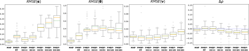
Figure 2: Comparison of performance metrics in the parameter recovery experiment across model fits: MHP (i.e. the data-generating process), PMBP-PP and PMBP-IC for varying interval sizes (1, 2, 5, 10 and 20). (left to right) RMSE for each parameter type $\{\boldsymbol{\alpha},\boldsymbol{\theta},\boldsymbol{\nu}\}$ and spectral radius estimation error $\Delta\rho$ . Samples are drawn from a 2-dimensional MHP with spectral radius $\rho(\boldsymbol{\alpha})=0.75$. Hyperparameters are $T=100$ and $N_{sequences}=50$. The mean and median estimates are indicated by the dashed green lines and solid orange lines, respectively.

We start by estimating the parameter recovery of a $2$-dimensional MHP process using $\textsc{PMBP}(2,1)$. We consider an MHP with $\rho(\boldsymbol{\alpha})=0.75$ and parameters $\alpha^{11}=0.32$, $\alpha^{12}=0.5$, $\alpha^{21}=0.3$, $\alpha^{22}=0.4$, $\theta^{11}=0.5$, $\theta^{12}=1.0$, $\theta^{21}=0.5$, $\theta^{22}=1.25$ and $\nu^{1}=\nu^{2}=0.1$ We set $\rho(\boldsymbol{\alpha})\in\{0.5,0.75,0.9\}$. We also test another parameter conbimation with $\rho(\boldsymbol{\alpha})=0.5$ (i.e. subcritical) and $\rho(\boldsymbol{\alpha})=0.9$ (i.e. approaching the critical regime) in Sec. 14.1 of the SI [22].

For a given parameter set, we sample $2500$ event sequences $\mathcal{H}^{1}_{100}\cup\mathcal{H}^{2}_{100}$ over the time interval $[0,100)$ using the MHP thinning algorithm [26]. Following a procedure similar to prior literature [6], we partition the 2500 event sequences into 50 groups, and each group of $N_{sequences}=50$ events is used for joint fitting, yielding a single parameter set estimate. In total, we obtain 50 sets of parameter estimates from the sample.

We construct the partially interval-censored dataset by interval-censoring $\mathcal{H}^{1}_{100}$, the first dimension of each realization in the timestamp dataset. Given a partition of $[0,100)$, we count the number of events on dimension $1$ that fall on each subinterval. We experiment with five observation window lengths to quantify the information loss of type (2) – intuitively, longer intervals lead to more significant information loss. We consider interval lengths of $1$, $2$, $5$, $10$ and $20$. For instance, with interval length of $2$ we tally event counts in the partition $\{[0,2),[2,4),\ldots,[98,100)\}$.

PMBP Log-Likelihood Functions: We fit the parameters of the $\textsc{PMBP}(d,e)$ model using two different versions of the likelihood function dependent on which dataset we use:

• timestamp dataset: we use the point-process log-likelihood on all dimensions, defined in Eq. 8: $\sum_{j=1}^{d}\mathscr{L}_{{\textsc{PP-LL}}}^{j}\left(\boldsymbol{\Theta};T\right)$.

• partially interval-censored dataset: we use the interval-censored log-likelihood on the $E$ dimensions and the point-process log-likelihood on the $E^{c}$ dimensions (see Eq. 6): $\sum_{j=1}^{e}\mathscr{L}_{{\textsc{IC-LL}}}^{j}\left(\boldsymbol{\Theta};T\right)+\sum_{j=e+1}^{d}\mathscr{L}_{{\textsc{PP-LL}}}^{j}\left(\boldsymbol{\Theta};T\right)$.

In what follows, we specify as $\textsc{PMBP}(d,e)$-PP and $\textsc{PMBP}(d,e)$-IC the $\textsc{PMBP}(d,e)$ model fit on the timestamp dataset and the partially interval-censored dataset, respectively. For brevity and whenever it is clear from context, we drop the dimensionalities $(d,e)$, and refer to the model fits as PMBP-PP and PMBP-IC. Also, for the PMBP-IC fits, we also specify $k$ – the length of the observation window – as PMBP-IC[$k$].

Metrics: We evaluate parameter recovery error with four error metrics: the root-mean-squared error (RMSE) of each PMBP parameter type $\{\hat{\boldsymbol{\alpha}},\hat{\boldsymbol{\theta}},\hat{\boldsymbol{\nu}}\}$ concerning the generating MHP parameters $\{\boldsymbol{\alpha},\boldsymbol{\theta},\boldsymbol{\nu}\}$ and the signed deviation $\Delta\rho=\rho(\hat{\boldsymbol{{\alpha}}})-\rho(\boldsymbol{{\alpha}})$ of the spectral radius.

Parameter Recovery Results: Fig. 2 shows RMSE$(\boldsymbol{\alpha}$), RMSE$(\boldsymbol{\theta}$), RMSE$(\boldsymbol{\nu}$) and $\Delta\rho$ across model fits. Within each subplot we have seven boxplots. The leftmost boxplot is the MHP fit, followed by the PMBP-PP fit (i.e., the PMBP fit on the timestamp dataset). The next five boxplots contain PMBP-IC fits of increasingly wider observation windows 1, 2, 5, 10 and 20. Note that the MHP fit represents the case where we do not have either model mismatch and interval censoring error.

In each subplot of Fig. 2, the gap between the first two boxplots (i.e. MHP vs. $\textsc{PMBP}(2,1)$ fitted on timestamp data) indicates model mismatch error; the gap between the second and third boxplots (i.e. $\textsc{PMBP}(2,1)$ fitted on timestamp data vs. partially interval-censored data) indicates interval censoring error. The gaps between succeeding boxplots indicate the effect of wider observation windows.

Fig. 2 shows three conclusions. First, model mismatch and interval censoring errors contribute to information loss relative to the MHP fit. Second, the approximation quality degrades as the observation window widens, indicating an increasing information loss of type (2). Third, for parameters $\boldsymbol{\alpha}$ and $\boldsymbol{\nu}$, the model mismatch error appears negligible; it is only for higher values of the observation window length ($\geq 5$) that the performance starts degrading due to information loss error. Both error types are present for $\boldsymbol{\theta}$. See Sec. 14.1 of the SI for individual parameter fits.

Though we observe that the generating parameters are not always correctly recovered, we see in the rightmost subplot of Fig. 2 that, interestingly, the spectral radius estimation error $\Delta\rho$ is close to zero regardless of model mismatch and exhibits only slight underestimation for wide observation windows. This is particularly relevant, as $\rho(\boldsymbol{\alpha})$ is a meaningful quantity relating to information spread virality (for social media diffusions), disease infectiousness (for epidemiology), or local seismicity (in seismology). The result indicates that even when individual parameter fits are inaccurate, the MHP regime is correctly identified.

Behavior of $\Delta\rho$ in Higher Dimensions: We further study the behavior of $\Delta\rho$ for varying MBP dimensions $e$ and model dimensionality $d$. We fix $T=100$ and $\rho(\boldsymbol{\alpha})=0.92$. Results for other error metrics are in Sec. 14.2 of the SI.

In the left subplot of Fig. 3, we fix $d=5$ and observe how the spectral radius error $\Delta\rho$ varies with the number of MBP dimensions $e$. Note that the leftmost boxplot represents the MHP fit (i.e., $e=0$). Interestingly, we see that all $\textsc{PMBP}(5,e),e<5$ flavors except the fully MBP case (i.e., $e=d=5$) can estimate the spectral radius as well as the MHP. The gap between the estimated spectral radii and the generating value (blue dashed line) is attributable to the difficulty of recovering MHP parameters in higher dimensions.

In the right subplot of Fig. 3, we fix $e=1$ and observe how the spectral radius error $\Delta\rho$ varies with the dimensionality $d$ of the $\textsc{PMBP}(d,1)$ process. The recovery error is generally low (except for $d=1$). However, we see that the magnitude of the error $\Delta\rho$ increases with increasing dimensionality starting from $d=2$, which is not surprising since the number of parameters increases quadratically as we increase the dimensionality of the process. We also see that fitting with a fully MBP model ($d=1$) does not show good recovery performance due to information loss, implying the necessity of having at least one cross-exciting dimension (i.e., $d-e\neq 0$).

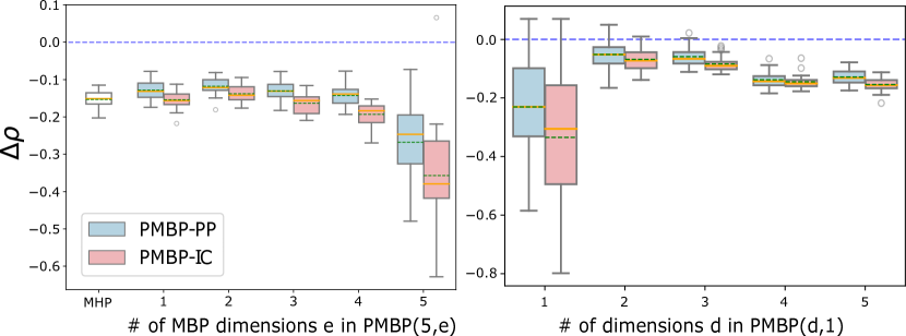
Figure 3: (Left) Relating the spectral radius estimation error $\Delta\rho$ of $\textsc{PMBP}(5,e)$ and the number of MBP dimensions $e$. Note that $\textsc{PMBP}(5,0)$ is the MHP (i.e. the data-generating process). (Right) Relating the spectral radius estimation error $\Delta\rho$ of $\textsc{PMBP}(d,1)$ and the model dimensionality $d$. In both plots, samples are drawn from a $d$-dimensional MHP with spectral radius $\rho(\boldsymbol{\alpha})=0.92$. Hyperparameters are $T=100$, $N_{sequences}=20$ and intervalsize=$1$. We fit two models for each PMBP column: $\textsc{PMBP}-\text{PP}$ (i.e. PMBP fit on timestamp data on all dimensions) and $\textsc{PMBP}-\text{IC}$ (i.e. PMBP fit on interval-censored data on the first $e$ dimensions and timestamp data on the last $d-e$ dimensions). The mean and median estimates are indicated by the dashed green lines and solid orange lines, respectively.

IV YouTube Popularity Prediction

In this section, we evaluate $\textsc{PMBP}(d,e)$’s performance in predicting the popularity of YouTube videos. For each video, we capture information about three dimensions – views, external shares and tweets linking to the videos – over the time period $[0,T^{train})$. We measure time in days relative to the time of posting on Youtube. The first two dimensions (the views and shares) are observed as daily counts, i.e., $E=\{views,shares\}$. The third dimension (tweets) is provided as event times, i.e. $E^{c}=\{tweets\}$. Given this data setup, we use $\textsc{PMBP}(3,2)$ to predict the daily counts of views and shares and the timestamp of the tweets posted over the period $[T^{train},T^{test})$.

Interval-Censored Forecasting with PMBP: To each YouTube video corresponds a partially interval-censored Hawkes realization. A straightforward approach to predict the unfolding of the realization during $[T^{train},T^{test})$ is to sample timestamps from $\textsc{PMBP}(3,2)$ on each of the three dimensions, conditioned on data before $T^{train}$; we then interval-censor the first two dimensions. In practice, sampling individual views takes considerable computational effort due to their high background rates, sometimes in the order of millions of views per day, and usually at least an order of magnitude larger than shares and tweets.

Below is an efficient procedure to calculate expected counts that leverages the compensator $\boldsymbol{\Xi}_{E}$ and requires sampling only the $E^{c}$ dimensions (i.e., tweets). Let $\mathcal{P}[T^{train},T^{test})=\bigcup_{i=1}^{P-1}[o_{i},o_{i+1}),$ where $o_{1}=T^{train}$ and $o_{P}=T^{test}$, be a partition of $[T^{train},T^{test})$.

1. Sample only the $E^{c}$ dimensions on $[T^{train},T^{test})$.

2. Compute expected counts on $\mathcal{P}[T^{train},T^{test})$ as $\{\boldsymbol{\Xi}_{E}(o_{i+1})$ - $\boldsymbol{\Xi}_{E}(o_{i})|i\in 1\cdots P-1\}$.

3. Compute the average of $\{\boldsymbol{\Xi}_{E}(o_{i+1})$ - $\boldsymbol{\Xi}_{E}(o_{i})|i\in 1\cdots P-1\}$ across samples.

More details of this scheme and a comparison with the standard method of sampling both $E^{c}$ and $E$ dimensions are provided in Sec. 13 of the SI [22].

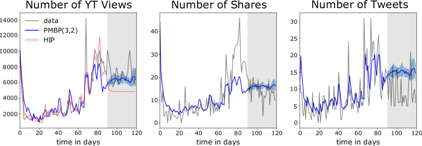
Figure 4: Comparison of fits and predictions of our proposal $\textsc{PMBP}(3,2)$ and the baseline HIP [13] for views (left), shares (center) and tweets (right) for a sample video from ACTIVE: a trailer for the 2014 movie Whiplash (id $7d\_jQycdQGo$). The first 90 days are used to fit model parameters, while the next 30 days (indicated by the gray shaded area) are unseen by the model and used for evaluation. HIP does not predict the share and tweet counts, as it treats these as exogenous inputs. The blue shaded area shows prediction uncertainty computed for the $\textsc{PMBP}(3,2)$ fits.

Dataset, Experimental Setup and Evaluation: We use two subsets of the ACTIVE dataset [13] for model fitting and evaluation. The first subset – dubbed ACTIVE $20\%$ – contains a $20\%$ random sample of the ACTIVE dataset [13], i.e., $2,834$ videos published between 2014-05-29 and 2014-12-26. The second subset – dubbed dynamic videos – contains videos with which users engage significantly during the test period. It is known that users’ attention to YouTube videos decays with time [12, 30]; therefore, the daily views of most ACTIVE videos hover around zero more than 90 days after their upload. We select the 585 dynamic videos with the standard deviations of the views, tweets, and shares counts on days $21-90$ higher than the median values on each of the three measures. Technical details of the filtering are in Sec. 15.1 of the SI [22].

For each video, we tune PMBP hyperparameters and parameters using the first $90$ days of daily view counts, share count to external platforms, and the timestamps of tweets that mention each video ($T^{train}=90$). It is known that generative models are suboptimal for prediction [10] and have to be adapted to the prediction task for better performance. Similar to HIP, we implement dimension weighting and parameter regularization in the likelihood. Full technical details of the fitting procedure are provided in Sec. 15.2 of the SI.

The days $91-120$ are used for evaluation ($T^{test}=120$). We measure prediction performance using the Absolute Percentile Error (APE) metric [13], which accounts for the long-tailness of online popularity – e.g., the impact of an error of 10,000 views is very different for a video getting 20,000 views per day compared to a video getting 2 million views a day. We first compute the percentile scale of the number of views accumulated between days 91 and 120. APE is defined as:

$$APE=|\text{Per}(\hat{N}_{120})-\text{Per}(N_{120})|$$

where $\hat{N}_{120}$ and $N_{120}$ are the predicted and observed number of views between days $91$ and $120$; the function $\text{Per}(\cdot)$ returns the percentile of the argument on the popularity scale.

Models and Baseline: We consider two $3$-dimensional PMBP models: $\textsc{PMBP}(3,2)$ and $\textsc{PMBP}(3,3)$. The former treats the tweets as a Hawkes dimension (see Definition 1) and is thus susceptible to computational explosion for high tweet counts given the quadratic complexity of computing cross- and self-excitation. The latter is an inhomogeneous Poisson process with no self- or cross-exciting dimension. We, therefore, fit $\textsc{PMBP}(3,2)$ solely on videos that have less than 1000 tweets on days $1-90$; we fit $\textsc{PMBP}(3,3)$ on all videos.

We use as a baseline the Hawkes Intensity Process (HIP), the current parametric state-of-the-art in popularity prediction discussed in Section II-A. HIP, however, is designed for use in a forecasting setup. That is, HIP requires the actual counts of tweets and shares in the prediction window $[T^{train},T^{test})$ to get forecasts for the view counts on $[T^{train},T^{test})$. To adapt HIP for the prediction setup (i.e., the tweets and shares are not available at test time), we feed HIP for each of the days 91-120 the time-weighted average of the daily tweet and share counts on $1-90$, i.e. $\frac{1}{\sum_{t=1}^{90}t}\sum_{t=1}^{90}t\cdot\#\text{tweets}(t)$ and $\frac{1}{\sum_{t=1}^{90}t}\sum_{t=1}^{90}t\cdot\#\text{shares}(t)$, which assigns a higher weight to more recent counts.

TABLE I: Performance comparison of $\textsc{PMBP}(3,3)$, $\textsc{PMBP}(3,2)$ and HIP on (a) a random sample that comprises $20\%$ of the videos in ACTIVE, and (b) the set of dynamic videos from ACTIVE: mean, median, and standard deviation of the percentile errors for each model. Best-performing score in bold.

	ACTIVE20% (n=2834)			DYNAMIC (n=585)
	PMBP (3,3)	PMBP (3,2)	HIP	PMBP (3,3)	PMBP (3,2)	HIP
Mean	4.82	7.36	8.12	10.86	7.28	9.31
Median	2.55	4.69	4.96	4.82	3.79	4.73
StdDev	7.13	8.34	9.89	14.24	9.58	11.89

Results: Fig. 4 illustrates the fits of $\textsc{PMBP}(3,2)$ and the baseline HIP [13] for a sample video from ACTIVE. Visibly, we see that $\textsc{PMBP}(3,2)$ and HIP have comparable fits of the popularity dynamics (left column) during the training period (unshaded area), but $\textsc{PMBP}(3,2)$ outputs a much tighter fit during the test period (gray shaded area). We also observe two advantages of PMBP. First, being a multivariate process that captures endogenous dynamics across its dimensions, $\textsc{PMBP}(3,2)$ provides a prediction for future share and tweet counts (center and left columns), in addition to the number of views. In contrast, HIP treats views (i.e. popularity) as exogenously driven by tweets and shares and thus can only predict the views’ dimension. Second, PMBP can quantify the uncertainty of the popularity prediction by sampling multiple unfoldings of a realization and computing the variance of the samples (shown as the blue shaded area in Fig. 4).

In Table I, we tabulate the mean, median and standard deviation of percentile errors for $\textsc{PMBP}(3,3)$, $\textsc{PMBP}(3,2)$, and HIP on ACTIVE $20\%$ and dynamic videos. We observe that the PMBP flavors consistently outperform the baseline HIP on both datasets. Visibly, on ACTIVE $20\%$, $\textsc{PMBP}(3,3)$ outperforms $\textsc{PMBP}(3,2)$. This is because most videos in ACTIVE $20\%$ do not exhibit much activity during the test period. Consequently, as a non-homogeneous Poisson process with no self-excitation, $\textsc{PMBP}(3,3)$ fits better such flat trends than the self-exciting $\textsc{PMBP}(3,2)$ and HIP models. On dynamic videos we see a reversal of performance ranking: $\textsc{PMBP}(3,2)$ performs best, followed by HIP and $\textsc{PMBP}(3,3)$. This result corroborates our claim in Section II-D that applying the heuristic of censoring event times leads to information loss. We see that $\textsc{PMBP}(3,2)$ (trained on tweet times) can better capture the popularity dynamics of the most complex videos (which are also the most interesting) compared to $\textsc{PMBP}(3,3)$ (trained on tweet counts).

V Interaction Between COVID-19 Cases and News

In the previous section we have validated the predictive power of the PMBP process. Here, we shift our attention to the interpretability of PMBP-fitted parameters. We showcase how PMBP can link online and offline streams of events by learning the interaction between the COVID-19 daily case counts and publication dates of COVID-19-related news articles for 11 different countries during the early stage of the pandemic.

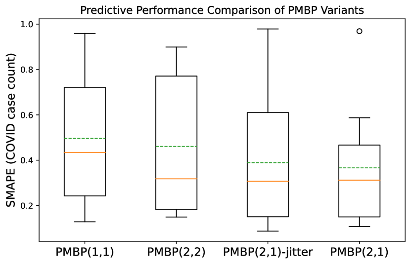
Figure 5: Performance comparison of $\textsc{PMBP}(1,1)$, $\textsc{PMBP}(2,2)$, $\textsc{PMBP}(2,1)$-jitter and $\textsc{PMBP}(2,1)$ on the COVID case count prediction task over our sample of 11 countries. The dashed line and solid line indicate the mean and median estimates, respectively.

Dataset: We curate and align two data sources.

The first dataset contains COVID daily case counts from the Johns Hopkins University [31]. The dataset is a set of date-indexed spreadsheets containing COVID reported case counts split by country and region. We focus on the following 11 countries: UK, USA, Brazil, China, France, Germany, India, Italy, Spain, Sweden, and the Philippines. We select the same countries as [3], to which we add the Philippines.

The second dataset contains timestamps of COVID-19-related news articles provided by the NLP startup Aylien [32]. This dataset is a dump of COVID-related English news articles from 440 major sources from November 2019 to July 2020. We filter the Aylien dataset for news articles that mention the selected 11 countries in the headline. To improve relevancy, for China, we also use several COVID-related keywords (such as coronavirus, covid and virus). Lastly, we only select articles from popular news sites with an Alexa rank of less than 150. Such news sources include Google News and Yahoo! News.

For each country, we fit $\textsc{PMBP}(2,1)$ with $E=\{cases\}$ and $E^{c}=\{news\}$. We consider as $t=0$ the first day on which a minimum of 10 cases were recorded. Except for China, which had cases as early as January 2020, the initial time for each country in our sample lies between February and March 2020. We only consider data until $t=120$, with time measured in days.

Incorporating News Information: To demonstrate the utility of news information in modeling COVID case counts, we compare the predictive performance of $\textsc{PMBP}(2,1)$ with three variants that leverage different granularities of news information. First, we compare with $\textsc{PMBP}(1,1)$ which does not use news information at all. Second, we compare with $\textsc{PMBP}(2,2)$ that uses daily aggregated news counts. Lastly, to test whether exact timing of news is important, we disaggregate daily news counts by adding a uniform jitter to each time, similar to what is done in [7], and fit $\textsc{PMBP}(2,1)$ to this dataset. We call this baseline $\textsc{PMBP}(2,1)$-jitter.

Similar to Section IV, we split our timeframe into a training period $[0,T^{train}=90)$ and a testing period $[T^{train},T^{test}=120)$. In our training period, we fit the models and perform hyperparameter tuning; in our testing period, we sample from the fitted models and evaluate performance. We measure performance using the Symmetric Mean Absolute Percentage Error (SMAPE), given by $SMAPE=\frac{1}{n}\sum_{t=1}^{n}\frac{|F_{t}-A_{t}|}{|A_{t}|+|F_{t}|},$ where $F_{t}$ and $A_{t}$ are the forecasted and actual values at time $t$, respectively.

Across our sample of 11 countries, we see in Fig. 5 that $\textsc{PMBP}(2,1)$ has the best performance compared to the three baselines and incorporating more granular news information leads to better predictive performance. We observe that the news-agnostic $\textsc{PMBP}(1,1)$ and the day aggregated $\textsc{PMBP}(2,2)$ models do not fit the data well and cannot capture the complex COVID case count dynamics. This supports our claim in Section II-D that application of data-altering heuristics leads to loss of information. However, by incorporating timestamped news information, we see significant performance improvement and we can match the trend in the case time series. We also see subtle performance improvement by incorporating exact news times ($\textsc{PMBP}(2,1)$-jitter vs. $\textsc{PMBP}(2,1)$).

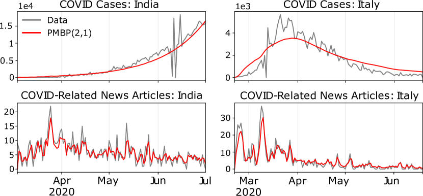
Figure 6: Observed and $\textsc{PMBP}(2,1)$-fitted daily COVID-19 case counts (top row) and COVID-19-related news articles (bottom row) for India (left column) and Italy (right) during the early stage of the outbreak.

TABLE II: $K$-means cluster centroids on the parameters obtained by fitting $\textsc{PMBP}(2,1)$ on the case count and news article dataset.

Cluster	$\theta^{11}$	$\theta^{12}$	$\theta^{21}$	$\theta^{22}$	$\alpha^{11}$	$\alpha^{12}$	$\alpha^{21}$	$\alpha^{22}$	$\nu^{1}$	$\nu^{2}$
UK, German, Spain	0.76	0.12	1.82	1.84	0.79	3.60	0.02	0.42	0.03	0.28
Brazil	0.13	0.01	1.89	2.46	1.08	5.48	0	0.38	0	1.47
China, France	0.62	4	1.70	3.55	0.68	0.73	0.3	0.39	0	0.05
US, Italy, Sweden	0.67	0.22	1.61	1.51	0.93	0.73	0.006	0.65	0.29	0.59
India, Philippines	0.12	2.28	2.15	1.88	1.35	0.54	0.007	0.58	0.08	0.66

Results: Fig. 6 shows the daily COVID-19 case counts and daily news article volume of the $\textsc{PMBP}(2,1)$ model fits for India and Italy. We show the plots for the other countries, the table of parameter estimates, and the goodness-of-fit analysis in Sec. 16 of the SI [22]. Visible from Fig. 6, $\textsc{PMBP}(2,1)$ captures well the dynamics of both countries. Based on the sample-based fit score introduced in the SI, the actual COVID-19 case counts for India and Italy fall within the model’s prediction interval for $97\%$ and $61\%$ of the time, respectively.

Cluster countries based on model fittings: The parameters capture different aspects of the interaction between news and cases. Here, we cluster the fitted parameter sets across countries to identify groups that have similar diffusion profiles. To render the scale of parameters comparable across countries, we rescale the maximum daily number of cases for each country over the considered timeframe to be 100, fit the $\textsc{PMBP}(2,1)$ model on this scaled data, and perform $K$-means clustering on the resulting parameter sets.

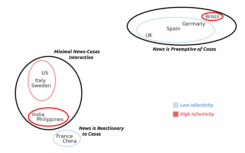
Figure 7: Labeled tSNE visualization of the clusters obtained from the fitted $\textsc{PMBP}(2,1)$ parameters across the 11 countries we consider.

The $k=5$ clusters are shown in Table II and visualized in Fig. 7 using t-SNE [33]. The first cluster (the UK, Germany, Spain) has high $\alpha^{12}$ and low $\alpha^{11}$. The second cluster – made solely of Brazil – has both a high $\alpha^{12}$ and a very high $\alpha^{11}$. With high $\alpha^{12}$, the two clusters contain countries where news strongly preempts cases. The third cluster (China and France) has a high $\alpha^{21}$ indicative of news playing a reactive role to cases. The fourth cluster (US, Italy, Sweden) and fifth cluster (India, Philippines) both have low $\alpha^{12}$ and $\alpha^{21}$, indicating little interaction between news and cases. We notice that COVID infectiousness is much higher in the fifth cluster (India, Philippines), with $\alpha^{11}$ greater than one (each case generates more than one case) and $\theta^{11}$ lowest across all clusters (slow decay, therefore long influence from cases to cases). Our fits indicate that India and the Philippines are countries particularly affected by COVID-19 in the early days.

VI Summary and Future Work

This work introduces the Partial Mean Behavior Poisson (PMBP) process, a generalization of the multivariate Hawkes process where we take the conditional expectation of a subset of dimensions over the stochastic history of the process. The motivation of our proposed approach comes from the need of fitting multivariate Hawkes process to partially interval-censored data. The multivariate Hawkes process cannot directly be used to fit this type of data, but the PMBP process can be used to approximate Hawkes parameters via a correspondence of parameters.

In this paper, we derive the conditional intensity function of the PMBP process by considering the impulse response to the associated LTI system. Additionally, we derive its regularity conditions which leads to a subcritical process; which we find generalizes regularity conditions of the multivariate Hawkes process and the previously proposed MBP process. The MLE loss function is also derived for the partially interval-censored setting.

To test the practicality of our proposed approach, we consider three empirical experiments.

First we test the capability of the PMBP process in recovering multivariate Hawkes process parameters in the partially interval-censored setting. By using synthetic data, we investigate the information loss from model mismatch and the interval-censoring of the timestamped data. Our results show that the fitted PMBP process can approximate the parameters and recover the spectral radius of the original multivariate Hawkes process used to generate the data.

Second, we demonstrate the predictive capability of the PMBP model by applying it to YouTube popularity prediction and showing that it outperforms the state-of-the-art baseline.

Third, to demonstrate interpretability of the PMBP parameters, we fit the process to a curated dataset of COVID-19 cases and COVID-19-related news articles during the early stage of the outbreak in a sample of countries. By inspecting the country-level parameters, we show that there is a demonstrable clustering of countries based on how news predominantly played its role: whether it was reactionary, preemptive, or neutral to the rising level of cases.

Future Work: There are three areas where future work can be explored. First, theoretical analysis on the approximation error of the model mismatch (i.e., fitting Hawkes data to the PMBP model) should be performed. In this work, we only perform an empirical evaluation of the information loss. Second, alternative schemes to approximate the conditional intensity should be investigated, as the current solution relies on the computationally heavy discrete convolution approximation. Lastly, given that the $\textsc{PMBP}(d,e)$ process, by construction, is not self- and cross-exciting in the $E$ dimensions, an open research question is whether we can construct a process that retains the self- and cross-exciting properties in all dimensions whilst also being flexible enough to be used in the partially interval-censored setting.

Pio Calderon Biography text here without a photo.

Alexander Soen Biography text here without a photo.

Marian-Andrei Rizoiu Biography text here without a photo.

VII Acknowledgments

Text describing those who supported your paper.

References

- [1] A. G. Hawkes, “Spectra of some self-exciting and mutually exciting point processes,” Biometrika, vol. 58, no. 1, pp. 83–90, 1971.
- [2] M.-A. Rizoiu, Y. Lee, S. Mishra, and L. Xie, “A Tutorial on Hawkes Processes for Events in Social Media,” arXiv:1708.06401 [cs, stat], Oct. 2017, arXiv: 1708.06401.
- [3] R. Browning, D. Sulem, K. Mengersen, V. Rivoirard, and J. Rousseau, “Simple discrete-time self-exciting models can describe complex dynamic processes: A case study of COVID-19,” PLoS ONE, vol. 16, no. 4 April, pp. 1–28, 2021, iSBN: 1111111111.
- [4] L. Shlomovich, E. Cohen, N. Adams, and L. Patel, “A Monte Carlo EM Algorithm for the Parameter Estimation of Aggregated Hawkes Processes,” arXiv:2001.07160 [stat], Jan. 2020, arXiv: 2001.07160.
- [5] D. Daley and D. Vere-Jones, An introduction to the theory of point processes. Vol. I, 2nd ed., ser. Probability and its Applications (New York). New York: Springer-Verlag, 2003.
- [6] M.-A. Rizoiu, A. Soen, S. Li, P. Calderon, L. Dong, A. K. Menon, and L. Xie, “Interval-censored Hawkes processes,” Journal of Machine Learning Research, vol. 23, no. 338, pp. 1–84, 2022. [Online]. Available: https://jmlr.org/papers/v23/21-0917.html
- [7] H. J. T. Unwin, I. Routledge, S. Flaxman, M.-A. Rizoiu, S. Lai, J. Cohen, D. J. Weiss, S. Mishra, and S. Bhatt, “Using Hawkes Processes to model imported and local malaria cases in near-elimination settings,” PLOS Computational Biology, vol. 17, no. 4, p. e1008830, Apr. 2021.
- [8] Q. Zhao, M. A. Erdogdu, H. Y. He, A. Rajaraman, and J. Leskovec, “SEISMIC: A Self-Exciting Point Process Model for Predicting Tweet Popularity,” Proceedings of the 21th ACM SIGKDD International Conference on Knowledge Discovery and Data Mining, pp. 1513–1522, Aug. 2015, arXiv: 1506.02594.
- [9] R. Kobayashi and R. Lambiotte, “TiDeH: Time-Dependent Hawkes Process for Predicting Retweet Dynamics,” arXiv:1603.09449 [physics], Mar. 2016, arXiv: 1603.09449.
- [10] S. Mishra, M. A. Rizoiu, and L. Xie, “Feature driven and point process approaches for popularity prediction,” International Conference on Information and Knowledge Management, Proceedings, vol. 24-28-Octo, pp. 1069–1078, 2016, iSBN: 9781450340731 _eprint: 1608.04862.
- [11] A. Zadeh and R. Sharda, “How can our tweets go viral? point-process modelling of brand content,” Information & Management, vol. 59, no. 2, p. 103594, 2022.
- [12] R. Crane and D. Sornette, “Robust dynamic classes revealed by measuring the response function of a social system,” Proceedings of the National Academy of Sciences of the United States of America, vol. 105, no. 41, pp. 15 649–15 653, 2008, _eprint: 0803.2189.
- [13] M. A. Rizoiu, L. Xie, S. Sanner, M. Cebrian, H. Yu, and P. Van Henteryck, “Expecting to be HIP: Hawkes intensity processes for social media popularity,” 26th International World Wide Web Conference, WWW 2017, pp. 735–744, 2017, iSBN: 9781450349130 _eprint: 1602.06033.
- [14] R. Krohn and T. Weninger, “Modelling online comment threads from their start,” in 2019 IEEE International Conference on Big Data (Big Data), 2019, pp. 820–829.
- [15] Q. Yan, S. Tang, S. Gabriele, and J. Wu, “Media coverage and hospital notifications: Correlation analysis and optimal media impact duration to manage a pandemic,” Journal of Theoretical Biology, vol. 390, pp. 1–13, Feb. 2016.
- [16] R. Chunara, J. R. Andrews, and J. S. Brownstein, “Social and News Media Enable Estimation of Epidemiological Patterns Early in the 2010 Haitian Cholera Outbreak,” The American Journal of Tropical Medicine and Hygiene, vol. 86, no. 1, pp. 39–45, Jan. 2012.
- [17] Q. Yan, Y. Tang, D. Yan, J. Wang, L. Yang, X. Yang, and S. Tang, “Impact of media reports on the early spread of COVID-19 epidemic,” Journal of Theoretical Biology, vol. 502, p. 110385, Oct. 2020.
- [18] M. Kirchner, “Hawkes and INAR( ) processes,” Stochastic Processes and their Applications, vol. 126, no. 8, pp. 2494–2525, Aug. 2016.
- [19] ——, “An estimation procedure for the Hawkes process,” Quantitative Finance, vol. 17, no. 4, pp. 571–595, Apr. 2017.
- [20] F. Cheysson and G. Lang, “Strong mixing condition for Hawkes processes and application to Whittle estimation from count data,” arXiv:2003.04314 [math, stat], Mar. 2020, arXiv: 2003.04314.
- [21] L. Shlomovich, E. A. K. Cohen, and N. Adams, “A Parameter Estimation Method for Multivariate Aggregated Hawkes Processes,” arXiv:2108.12357 [stat], Aug. 2021, arXiv: 2108.12357.
- [22] “Appendix: Linking across data granularity: Fitting multivariate hawkes processes to partially interval-censored data,” 2023, https://bit.ly/45huSRl.
- [23] C. L. Phillips, J. M. Parr, E. A. Riskin, and T. Prabhakar, Signals, systems, and transforms. Prentice Hall Upper Saddle River, 2003.
- [24] Y. Ogata, “The asymptotic behaviour of maximum likelihood estimators for stationary point processes,” Annals of the Institute of Statistical Mathematics, vol. 30, no. 2, pp. 243–261, Dec. 1978.
- [25] A. Wächter and L. T. Biegler, “On the implementation of an interior-point filter line-search algorithm for large-scale nonlinear programming,” Mathematical Programming, vol. 106, no. 1, pp. 25–57, Mar. 2006.
- [26] Y. Ogata, “On Lewis’ simulation method for point processes,” IEEE Transactions on Information Theory, vol. 27, no. 1, pp. 23–31, Jan. 1981.
- [27] K. Fokianos, A. Rahbek, and D. Tjøstheim, “Poisson autoregression,” Journal of the American Statistical Association, vol. 104, no. 488, pp. 1430–1439, 2009.
- [28] A. Eckner, “A framework for the analysis of unevenly spaced time series data,” Preprint. Available at: http://www. eckner. com/papers/unevenly_spaced_time_series_analysis, p. 93, 2012.
- [29] K. Rehfeld, N. Marwan, J. Heitzig, and J. Kurths, “Comparison of correlation analysis techniques for irregularly sampled time series,” Nonlinear Processes in Geophysics, vol. 18, no. 3, pp. 389–404, 2011.
- [30] S. Wu, M.-A. Rizoiu, and L. Xie, “Estimating Attention Flow in Online Video Networks,” Proceedings of the ACM on Human-Computer Interaction, vol. 3, no. CSCW, pp. 1–25, nov 2019.
- [31] E. Dong, H. Du, and L. Gardner, “An interactive web-based dashboard to track COVID-19 in real time,” The Lancet Infectious Diseases, vol. 20, no. 5, pp. 533–534, May 2020.
- [32] Aylien, “AYLIEN Coronavirus Dataset,” 2020.
- [33] L. van der Maaten and G. Hinton, “Visualizing data using t-sne,” Journal of Machine Learning Research, vol. 9, no. 86, pp. 2579–2605, 2008.