Load Restoration in Islanded Microgrids:
Formulation and Solution Strategies

Abstract

Adverse circumstances such as extreme weather events can cause significant disruptions to normal operation of electric distribution systems (DS), which includes isolating parts of the DS due to damaged transmission equipment. In this paper, we consider the problem of load restoration in a microgrid (MG) that is islanded from the upstream DS. The MG contains sources of distributed generation such as microturbines and renewable energy sources, as well as energy storage systems (ESS). We formulate the load restoration task as a non-convex optimization problem. This problem embodies the physics of the MG by leveraging a branch flow model, while incorporating salient phenomenon in islanded MGs such as the need for internal frequency regulation, and complementarity requirements arising in ESS operations. Since the formulated optimization problem is non-convex, we introduce a convex relaxation which can be solved through model predictive control as a baseline method. However, in order to solve the problem considering its full non-convexity, we leverage a policy-learning method called constrained policy optimization, a tailored version of which is used as our proposed algorithm. The aforementioned approaches, along with an additional deep learning method are compared through extensive simulations.

Electric power networks, load restoration, islanded microgrids, convex relaxation, constrained policy optimization.

1 Introduction

Extreme weather events such as wildfires, hurricanes, and winter storms pose a big threat to reliable operation of electric distribution systems (DS) [1]. Those events can disrupt the operation of DS by damaging electric transmission equipment such as overhead power lines, thereby curbing the delivery of electric power. Traditionally, DS have been designed to be reliable during nominal operations and in face of predictable off-nominal operating conditions. Recently, a new paradigm of resilience is being explored by the power engineering community, which posits that a DS must be capable of rapidly recovering to a state of nominal operations post extreme weather events [2]. As localized distribution systems, microgrids (MGs) facilitate system resilience, which are equipped with distributed power generation including microturbines (MTs) and renewable energy sources (RES). RES may contain energy from photovoltaics, wind turbines, geothermal sources, etc. The intermittent nature of power production of RESs necessitates energy storage systems (ESS).

Thus, MGs have sources of power generation as well as energy storage. They are an ideal candidate for restoring power demand for loads such as residential homes, industries and critical services such as hospitals, especially when they become disconnected (islanding mode) from the upstream DS. Coordination of distributed generation sources within islanded MGs occurs through a bi-hierarchical control scheme: the lower-level primary control allows for communication-free fast response to disturbances, while the higher level secondary & tertiary controls are used to generate setpoints for primary control. The latter act over longer timescales while leveraging communication infrastructure available to the MG [3]. Secondary and tertiary control in MGs is achieved with a MG controller (MGC) [4], which is a central computer capable of communicating with and controlling generation and storage elements in the MG. Since load restoration involves coordination of sources and loads in face of constraints arising from to network physics and finite generation capacities, the MGC’s algorithm is best posed as an optimization problem [5], which can be solved in real-time by the MGC.

Load restoration, when posed as an optimization problem, features several unique characteristics which inform strategies to solve it. The first challenge arises from the non-convexity of AC power flow (ACPF) equations, which embody the physics of power transfer. Since the ACPF equations are a part of the constraints in load restoration, any solution thereof cannot be certified as globally optimal [6]. In this paper, we use the DistFlow equations instead of ACPF equations, since the former is equivalent to the latter in power networks with radial topologies [7], which is typical of MGs. The DistFlow equations, which lend themselves to intuitive convex relaxations, were first introduced in literature by Baran and Wu [8]. The second challenge involves discrete decisions which must be made as a part of load restoration process. An important example is the principle of ESS complementarity, which states that an ESS may not simultaneously charge and discharge at any given time [9]. This principle has conventionally been encoded using nonconvex [10] or integer [11] constraints, or enforced through penalty terms in the objective function [12]. The third challenge is based on the observation that in islanded MGs, there is no external source of AC frequency regulation and therefore, it must be done using internal sources such as voltage source inverters (VSI). Thus, the dependence of voltages and AC frequency on real and reactive power generation must be modeled as a (possibly convex) constraint [13]. The last challenge involves the uncertainty in forecasts of renewable sources, which render the calculated solution sub-optimal as the quality of forecasts degrade substantially.

As shown in the sequel, formulating load restoration as an optimization problem considering the aforementioned challenges results in a non-convex nonlinear program (NLP) defined over multiple time steps. The non-convexity implies that there are no guarantees on whether a candidate feasible solution is globally optimal. Two approaches may be used to remedy this drawback: use of heuristic solution algorithms, or relaxation of the problem into a more tractable form. For the latter approach, it is desirable to generate a linear or convex relaxation of the problem, which can then be solved through model predictive control (MPC). MPC is a popular technique for optimal control of dynamical systems wherein a control task, posed as an optimization problem defined over a long time horizon is decomposed into smaller sequential subproblems and solved. MPC has been applied to several applications such as voltage stability assurance [14], demand response in industrial loads [15], Volt-VAR control [16], and scheduling PV storage systems [17].

The other approach is to use heuristic solution strategies. In this paper, we consider reinforcement learning (RL) for this purpose. RL, and deep RL (in which deep neural networks are used to approximate various functions used in RL) are concerned with determining actions which an agent interacting with an environment should take to maximize it accumulated reward. Over the last decade, RL has been considered for various power systems applications such as Volt-VAR control [18], EV charge scheduling [19], power management in networked MGs [10], and optimal control of ESS in MGs [20]. A specific RL algorithm which can be useful in the current setting is constrained policy optimization (CPO) [21]. CPO aims to find a policy which takes as input the current system state and outputs the optimal action with respect to the reward, while satisfying multiple constraints on state and action. The policy is be represented as a neural network, which can be trained [22] such that its outputs approach optimality. While CPO has recently been considered for power system applications [10, 23], significant challenges remain in tailoring the training procedure of CPO to a given application. Tailoring CPO for load restoration is considered in this paper.

We conclude this section by mentioning other strategies used in load restoration literature. Many frameworks for load restoration consider reconfigurable MGs with inelastic loads, wherein the decision variable include discrete switching actions and dispatch of generation. Such problems may be solved by posing it as a maximum coverage problem [24], or using spanning tree search [25]. On the contrary, we consider a fixed-topology radial MG and elastic loads, while focusing on optimum dispatch of MTs, RESs, and ESSs. Such formulations have been solved in literature using stochastic optimization [11], scenario generation and pruning [26], and RL aided by power flow simulators [27]. Many formulations also assume additional infrastructure such as mobile ESSs [28]. We restrict our attention to cases without specialized infrastructure, and do not consider explicit scenario generation: the CPO agent implicitly generates scenarios as it steers the grid along different trajectories during simulation-based training.

Motivation

The principal motivation of this paper is to compare performance of a RL-based MG controller for load restoration over conventional optimization-based techniques such as MPC. There are two advantages which RL has over MPC: firstly, neural-network based controllers (alternatively known as policy) trained with RL require significantly lower computational resources for implementation as compared to optimization solvers. Secondly, since RL involves learning from exploratory experience, it is possible for the policy to learn mispredictions in forecasts, thereby increasing robustness of generated solutions. However, the downside to RL is that it produces black-box models which may generate suboptimal or infeasible solutions. To that end, we seek to tailor CPO policy training such that solutions generated are feasible with respect to DistFlow equations and other operational constraints. This would also alleviate the biggest drawback of interior-point methods (IPM) conventionally used to solve MPC: non-convexity and complementarity constraints may lead to ill-conditioning or exponential solve times of IPM-based solvers.

Contribution statement

In this paper, we consider load restoration for a fixed-topology islanded MG as an optimization problem, in which we incorporate constraints arising from different elements participating in the MG. As a baseline solution strategy we consider MPC, for which we propose a convex relaxation of the problem. However, in order to solve the exact problem approximately, we consider CPO, whose training procedure is adapted specifically for load restoration. Finally, we compared the MPC and CPO solution quality and performance through simulations, and both these methods are compared to a brute-force learning approach from a dataset.

We make a few standing assumptions for our formulation of load restoration. First, we assume that the MG has a fixed radial topology, and line parameters such as resistance and reactance are known. Second, we assume that the loads are flexible i.e. they can accept a fraction of the load power demanded, and we also assume that the RES output can be fractionally curtailed. Third, we consider the load demands to be static and fixed over the entire duration of the restoration procedure, while forecasts of RES outputs are assumed to have errors over the same duration.

The main contributions of our work are summarized as follows:

1. Alongside existing relaxations for DistFlow equations, we present new convex relaxations for ESS complementarity and the dependence of inverter voltages on real power. These relaxations serve to render MPC sub-problems convex, thereby allowing use of convex optimization solvers for solving the same.

2. Alternatively, in order to solve the unrelaxed load restoration problem, we consider the use of CPO. Training a policy with CPO involves updating learnable weights of the policy using a quadratically constrained optimization problem multiple times for every episode. In Proposition 1 and Lemma 4.3, we present a tailored method for efficiently calculating coefficients of said optimization problem.

In Section 5, we compare the relaxed MPC controller with the CPO policy. The comparisons entail verifying the performance of both under erroneous forecasts of RES output. Furthermore, we compare the feasibility gaps accrued due to the MPC relaxation with those resulting from the CPO policy.

The remainder of the paper is organized as follows. Section 2 presents the problem formulation of load restoration. Section 3 shows how the problem can be relaxed and solved by MPC. Section 4 details our proposed CPO approach along with a procedure on how to train the CPO policy. Section 5 compares the solutions obtained by the two approaches, with a third approach learning the solutions generated by CPO with a deep neural network. Section 6 concludes this work. All detailed proofs of lemmas and propositions are deferred to the Appendix.

Notation

The notations $\mathbb{R}$, $\mathbb{C}$, $\mathbb{N}$, and $\mathbb{R}_{+}$ denote the sets of real numbers, complex numbers, natural numbers, and non-negative reals respectively. For a complex number $c\in\mathbb{C}$, $\Re(c)$ and $\Im(c)$ denotes its real and imaginary parts. $\text{conv}(\mathcal{A})$ is the convex hull of set $\mathcal{A}$. $D_{\text{KL}}\left(p_{1}\lVert p_{2}\right)$ denotes the KL-divergence between probability distributions $p_{1}$ and $p_{2}$. For a real number $a\in$, $[a]^{+}$ and $[a]^{-}$ denote $\max\{a,0\}$ and $\max\{-a,0\}$ respectively. Boldface variables represent vectors and matrices. $\mathbf{a}^{\top}$ and $\mathbf{a}^{H}$ represent the transpose, and complex conjugate transpose of vector $\mathbf{a}$ respectively. $\mathbf{I}^{\text{id}}_{n}$ is the identity matrix of size $n\times n$. $\mathbf{a}\preceq\mathbf{b}$ denotes the elementwise inequality between two vectors. $\mathbf{A}\otimes\mathbf{B}$ denotes the Kronecker product of $\mathbf{A}$ and $\mathbf{B}$. $\left\lVert\mathbf{a}\right\rVert_{2}$ denotes the 2-norm of vector $\mathbf{a}$. $\mathcal{N}(\boldsymbol{\mu},\boldsymbol{\Sigma})$ denotes a multivariate Gaussian distribution with mean vector $\boldsymbol{\mu}$ and covariance matrix $\boldsymbol{\Sigma}$. For a random variable $X$, $\mathbb{E}\left[X\right]$ denotes its expectation.

2 Load Restoration Problem Formulation

Consider a MG that is islanded from the upstream DS due to an extreme weather event. Let the MG be represented by a directed graph $\mathcal{G}=(\mathcal{N},\mathcal{E})$, where $\mathcal{N}$ represents the set of buses and $\mathcal{E}$ is the set of power lines. We assume that $\mathcal{G}$ is a radial network, i.e., $\mathcal{G}$ is a tree. $\mathcal{N}$ is the union of disjoint sets $\mathcal{N}^{\text{L}}$, $\mathcal{N}^{\text{MT}}$, $\mathcal{N}^{\text{RES}}$, and $\mathcal{N}^{\text{ESS}}$, where $\mathcal{N}^{\text{L}}$ represents the load buses, $\mathcal{N}^{\text{MT}}$ represents the buses connected to a MT, $\mathcal{N}^{\text{RES}}$ represents the buses with RES, and $\mathcal{N}^{\text{ESS}}$ represents the buses connected to an ESS. We consider the load restoration problem over a time horizon of $\mathcal{T}\stackrel{{\scriptstyle\Delta}}{{=}}\{1,2,\cdots,T\}$, and time steps are indexed by $t$. We let $s_{i,t}\in\mathbb{C}$ and $v_{i,t}\in\mathbb{R}_{+}$ denote the complex power injection and squared magnitude of voltage phasor at bus $i\in\mathcal{N}$ respectively at time $t$. For every line $(i,j)\in\mathcal{E}$, we let $S_{ij,t}\in\mathbb{C}$, and $l_{ij,t}\in\mathbb{R}_{+}$ denote the sending-end complex power flow and squared magnitude of the current phasor, respectively. For buses $i$ and $j$, notation $i\rightarrow j$ indicates the presence of a power line in between, i.e. $(i,j)\in\mathcal{E}$. Note that any equation involving the index $t$, unless stated otherwise, is assumed to hold for all $t\in\mathcal{T}$.

Objective function

The objective is to maximize load restoration while minimizing MT fuel consumption. To that end, an appropriate objection function can be represented as

$$J_{\mathcal{T}}\stackrel{{\scriptstyle\Delta}}{{=}}\sum_{t\in\mathcal{T}}\left(\sum_{i\in\mathcal{N}^{\text{L}}}C^{\text{L}}_{i,t}(\Re(s_{i,t}))+\sum_{i\in\mathcal{N}^{\text{MT}}}C^{\text{MT}}_{i,t}(\Re(s_{i,t}))\right),$$ (1)

where the (possibly time varying) functions $C^{L}$ and $C^{\text{MT}}$ are convex functions wherein the former is non-increasing and the latter non-decreasing in their respective arguments. The objective function is meant to incentivize the amount of load power restored, while disincentivizing power produced from MT in favor of utilizing ESSs or RESs. In practice, $C^{L}$ is often linear with coefficients representing priority order of load restoration, while $C^{\text{MT}}$ can be linear or negative convex quadratic.

Power flow constraints

Let $z_{ij}\in\mathbb{C}$ represent the impedance of line $i\rightarrow j$. We use the DistFlow equations for quantifying the power flows that are given as follows:

$$s_{j} =\sum_{j\rightarrow k}S_{jk,t}-\sum_{i\rightarrow j}\left(S_{ij,t}-z_{ij}l_{ij,t}\right),\forall j\in\mathcal{N}$$ (2a)

$$v_{j,t} =v_{i,t}-\Re(\bar{z}_{ij}S_{ij,t})+|z_{ij}|^{2}l_{ij,t},\,\forall i\rightarrow j$$ (2b)

$$v_{i,t}l_{ij,t}=|S_{ij}|^{2},\;\forall i\rightarrow j.$$ (2c)

It is known that in radial networks, voltage angles can be recovered from any solution of equations (2a) to (2c) [7, Theorem 2]. The voltage and current constraints at each bus and line respectively, needed for nominal operation of the MG, are codified as follows:

$$\underline{v}\leq v_{i,t}\leq\bar{v},\;\forall i\in\mathcal{N},$$ (3)

$$l_{ij,t}\leq\bar{l}_{ij},\;\forall i\rightarrow j.$$ (4)

MT Constraints

The power generation of each MT is subject to constraints on per-time step generation, as well as those on rates of ramping up/down. They are given as

$$\underline{P}^{\text{MT}}_{i}\leq\Re(s_{i,t})\leq\bar{P}^{\text{MT}}_{i},\;\forall i\in\mathcal{N}^{\text{MT}},$$ (5a)

$$\underline{P}^{\text{MT}}_{\text{rd}}\leq\Re(s_{i,t})-\Re(s_{i,t-1})\leq\bar{P}^{\text{MT}}_{\text{ru}},\forall i\in\mathcal{N}^{\text{MT}},$$ (5b)

$$\Re(s_{i,1})\leq\bar{P}^{\text{MT}}_{\text{ru}},\;\forall i\in\mathcal{N}^{\text{MT}},$$ (5c)

wherein (5b) holds for all $t\in\mathcal{T}\setminus\{1\}$. Each MT is assumed to have a fixed amount of fuel at the beginning of $\mathcal{T}$. This constrains the total amount of real power produced over $\mathcal{T}$ as $\left(\sum_{t\in\mathcal{T}}\Re(s_{i,t})\right)\tau_{i}\leq E_{i},\;\forall i\in\mathcal{N}^{\text{MT}}$, wherein $E_{i}$ is the total fuel initially available at MT $i$, and $\tau_{i}$ is the fuel-to-power conversion factor. The total fuel constraint can be reformulated as a recursive relation by denoting with $\varsigma_{i,t}$ the amount of fuel remaining in MT $i$ at time $t$ and observing that

$$\varsigma_{i,t}=\varsigma_{i,t-1}-\tau_{i}\Re(s_{i,t}),\;\forall i\in\mathcal{N}^{\text{L}}$$ (6a)

$$\varsigma_{i,T}\geq 0,\;\forall i\in\mathcal{N}^{\text{L}}$$ (6b)

with the initial condition $$\varsigma_{i,0}=E_{i}$$.

ESS Constraints

Each ESS is an energy reservoir which may discharge power into the MG when required, and otherwise charge in order to replenish its energy reserves. We denote by (SoC) $\mathcal{S}_{i,t}$ the state of charge (SoC) of ESS $i$ at time step $t$, which takes values in $[\underline{\mathcal{S}}_{i},\bar{\mathcal{S}}_{i}]$. Letting $P^{\text{ch}}_{i,t}$ and $P^{\text{dis}}_{i,t}$ denote the charge and discharge powers of the same, the power input/output constraints of the ESS are:

$$0\leq P^{\text{dis}}_{i,t}\leq\bar{P}_{i}^{\text{dis}},\;0\leq P^{\text{ch}}_{i,t}\leq\bar{P}_{i}^{\text{ch}},\;\forall i\in\mathcal{N}^{\text{ESS}},$$ (7a)

$$P^{\text{ch}}_{i,t}P^{\text{dis}}_{i,t}=0,\;\forall i\in\mathcal{N}^{\text{ESS}},$$ (7b)

$$\Re(s_{i,t})=P^{\text{dis}}_{i,t}-P^{\text{ch}}_{i,t},\;\forall i\in\mathcal{N}^{\text{ESS}}.$$ (7c)

Note that the (7b) denotes the complementarity constraint, which may alternatively be denoted as an integer constraint using a charge/discharge indicator variable. The evolution of $\mathcal{S}_{i,t}$ is given as:

$$\mathcal{S}_{i,t}=\mathcal{S}_{i,t-1}+\eta^{\text{ch}}_{i}P^{\text{ch}}_{i,t}\Delta_{t}-\frac{1}{\eta^{\text{dis}}_{i}}P^{\text{dis}}_{i,t}\Delta_{t},\;\forall i\in\mathcal{N}^{\text{ESS}},$$ (8a)

$$\mathcal{S}_{i,0}=\mathcal{S}^{\text{init}}_{i},\;\mathcal{S}_{i,t}\in[\underline{\mathcal{S}}_{i},\bar{\mathcal{S}}_{i}],\;\forall i\in\mathcal{N}^{\text{ESS}},$$ (8b)

wherein (8a) holds for all $t\in\mathcal{T}$, $\eta^{\text{ch}}_{i}\in(0,1]$ and $\eta^{\text{dis}}_{i}\in(0,1]$ denote the charge and discharge efficiency for ESS $i$, $\Delta_{t}$ denotes the time duration corresponding to each time step, and $\mathcal{S}^{\text{init}}_{i}$ denotes the initial SoC of ESS $i$. Considering other factors such as battery temperature, the efficiencies $\eta^{\text{ch}}_{i}$ and $\eta^{\text{dis}}_{i}$ can be modeled as time-varying [29].

RES Constraints

Since the power output of RES is stochastic in nature and cannot be predicted with certainty ahead-of-time, a forecast $\hat{P}^{\text{RES}}_{i,t}$ is used as a stand-in for the actual output. We assume each RES has the capability to curtail its power output, and denote by $\kappa_{i,t}\in[0,1]$ the curtailment ratio of the real power. The RES real power constraint is given as

$$\Re(s_{i,t})=(1-\kappa_{i,t})\hat{P}^{\text{RES}}_{i,t},\;\forall i\in\mathcal{N}^{\text{RES}}.$$ (9)

Reactive Power and Droop Bus Constraints

The MT, RES, and ESS buses may be interfaced to the MG through inverters which convert DC to AC power. Such inverters are capable of supplying and absorbing reactive power to and from the MG, constrained as

$$|\Im(s_{i,t})|\leq\bar{Q}_{i},\;\forall i\in\mathcal{N}^{\text{MT}}\cup\mathcal{N}^{\text{ESS}}\cup\mathcal{N}^{\text{RES}},$$ (10)

where $\bar{Q}_{i}$ is the nameplate capacity of the inverter at bus $i$. Other representations of inverter capacity that limit the total apparent power of the inverter (by way of an upper bound on $|s_{i,t}|$) may also be used in lieu of (10).

Many inverters in MGs may operate on the principle of droop control, also referred to as voltage source inverter control, wherein the inverter acts as an AC voltage source, with voltage and frequency depending on the real and reactive power output. Letting $\mathcal{N}^{\text{droop}}\subset\left\{\mathcal{N}\setminus\mathcal{N}^{\text{L}}\right\}$ denote the set of generation buses operating on droop control (‘droop buses’), and $\omega_{t}$ denote the system frequency at time $t$, the droop bus constraints are given as [30]:

$$\omega_{t}=\omega_{i}^{*}-k_{P}(\Re(s_{i,t})-P^{*}_{i}),\;\forall i\in\mathcal{N}^{\text{droop}}$$ (11a)

$$\sqrt{v_{i,t}}=\sqrt{v^{*}_{i}}-k_{Q}(\Im(s_{i,t})-Q^{*}_{i}),\;\forall i\in\mathcal{N}^{\text{droop}},$$ (11b)

$$\underline{\omega}\leq\omega_{t}\leq\bar{\omega},$$ (11c)

wherein $\omega^{*}$, $v_{i}^{*}$, $P_{i}^{*}$, and $Q_{i}^{*}$ are operational setpoints of the inverter, while $k_{P}$ and $k_{Q}$ are the droop constants. Since the MG receives no frequency signals from the upstream DS during islanding, droop buses are essential for internal frequency regulation of the system, which is achieved through constraint (11c).

Load Constraints

We let time-varying forecasts of active and reactive power demands of the loads be denoted by $\hat{P}^{\text{L}}_{i,t}$ and $\hat{Q}^{\text{L}}_{i,t}$ respectively. We let $\rho_{i,t}\in[0,1]$ denote the pickup ratio (i.e. ratio of load served with respect to demand) of load $i\in\mathcal{N}^{\text{L}}$ at time $t$.. Assuming a constant power factor, we have the constraints

$$\Re(s_{i,t})=-\rho_{i,t}\hat{P}^{\text{L}}_{i,t},\,\;\Im(s_{i,t})=-\rho_{i,t}\hat{Q}^{\text{L}}_{i,t},\,\forall i\in\mathcal{N}^{\text{L}}.$$ (12)

A monotonically increasing pickup ratio is preferable over frequent dropping of loads already picked up. This is ensured by the almost-monotonic load restoration constraint,

$$\rho_{i,{t}}-\rho_{i,t-1}\geq-\epsilon,\;\forall i\in\mathcal{N}^{\text{L}},\forall t\in\mathcal{T}\backslash\{1\},$$ (13)

where parameter $\epsilon\geq 0$ allows for a small leeway in monotonicity of load pickup, and is chosen by the system operator.

Optimization Problem

We collect all decision variables at time $t$ as

$$\mathcal{X}_{t}\stackrel{{\scriptstyle\Delta}}{{=}} \big{\{}\left\{s_{i,t},v_{i,t}\right\}_{i\in\mathcal{N}},\left\{S_{ij,t},l_{ij,t}\right\}_{i\rightarrow j},\left\{\zeta_{i,t}\right\}_{i\in\mathcal{N}^{\text{MT}}},$$

$$\left\{\mathcal{S}_{i,t},P^{\text{ch}}_{i,t},P^{\text{dis}}_{i,t}\right\}_{i\in\mathcal{N}^{\text{ESS}}},\left\{\kappa_{i,t}\right\}_{i\in\mathcal{N}^{\text{RES}}},\left\{\rho_{i,t}\right\}_{i\in\mathcal{N}^{\text{L}}},\omega_{t}\big{\}}.$$

To this end, the optimization problem to be solved by the MGC is given as

$$\max\limits_{\left\{\mathcal{X}_{t}\right\}_{t\in\mathcal{T}}}\quad \eqref{eq:objective}$$ (14a)

s.t. $$\eqref{eq:PF}-\eqref{eq:load_monotonicity}.$$ (14b)

Obtaining an optimal solution to (14) allows the MGC to implement said solution for load restoration. Note that the constraints (2c), (7b), and (11b) are non-convex, thereby making (14) overall non-convex and devoid of global optimality guarantees.

3 Convex Relaxation and Solution using Model Predictive Control

In this section, we consider convex relaxations to problem (14) which make it amenable to MPC. The MPC approach involves solving (14) over subhorizons of $\mathcal{T}$, followed by using the subhorizon-optimal solutions to construct a near-optimal solution over $\mathcal{T}$ [31]. The non-convexity arising from DistFlow equations (2c) can be addressed using a well-studied second-order cone relaxation $v_{i,t}l_{ij,t}\geq|S_{ij}|^{2}$, equivalently written as a second-order cone,

$$\left\lVert\begin{bmatrix}2\Re(S_{ij,t})&2\Im(S_{ij,t})&l_{ij,t}-v_{i,t}\end{bmatrix}^{\top}\right\rVert_{2}\leq l_{ij,t}+v_{i,t}.$$

We use the above relaxation for the MPC formulation. Next, we consider the droop bus equation (11b) which is non-convex due to presence of the term $\sqrt{v_{i,t}}$. It can be relaxed to a second-order cone as follows.

Lemma 1 (Convex relaxation of (11b))

The constraint $\sqrt{v_{i,t}}=\sqrt{v_{i}^{*}}-k_{Q}(\Im(s_{i,t})-Q_{i}^{*})$ can be relaxed to a second-order cone given as

$$\left\lVert\begin{bmatrix}\left(\sqrt{v_{i}^{*}}-k_{Q}(\Im(s_{i,t})-Q_{i}^{*})\right)&v_{i,t}&\frac{1}{2}\end{bmatrix}^{\top}\right\rVert_{2}\leq v_{i,t}+\frac{1}{2}.$$

Proof 3.1.

See Appendix  .1.

Lastly, we consider the non-convex ESS CC constraints. We address the non-convexity by relaxing the joint feasible region of $P^{\text{ch}}_{i,t}$ and $P^{\text{dis}}_{i,t}$ to its convex hull, whose closed form is given as follows.

Lemma 3.2 (Convex hull of nonconvex ESS CC feasible set).

Define the set $\mathcal{P}_{i}^{t}\stackrel{{\scriptstyle\Delta}}{{=}}\left\{(P^{\text{ch}}_{i,t},P^{\text{dis}}_{i,t})\,|\,\eqref{eq:charge}-\eqref{eq:complementarity}\right\}$. Then, the convex hull of $\mathcal{P}_{i}^{t}$ is given as

$$\mathcal{P}_{i}^{t,\text{conv}}= \left\{(P^{\text{ch}}_{i,t},P^{\text{dis}}_{i,t})\,\bigg{|}\,P^{\text{ch}}_{i,t}\geq 0,P^{\text{dis}}_{i,t}\geq 0,\frac{P^{\text{ch}}_{i,t}}{\bar{P}^{\text{ch}}_{i}}+\frac{P^{\text{dis}}_{i,t}}{\bar{P}^{\text{dis}}_{i}}\leq 1\right\}.$$

Proof 3.3.

See Appendix .2.

The relaxation of CC presented in Lemma 3.2 replaces the constraints (7). A concern is that the relaxed solution may be physically unimplementable due to non-complementarity. However, based on results presented in [32], it is possible to recover a charge/discharge schedule which results in the same power injections (7c), while satisfying CC. For an ESS $i\in\mathcal{N}^{\text{ESS}}$, consider a charge/discarge schedule satisfying constraints in Lemma 3.2, given as $\mathbf{P}_{i}^{\text{ch}}\stackrel{{\scriptstyle\Delta}}{{=}}\{P_{i,t}^{\text{ch}}\}_{t\in\mathcal{T}}$ and $\mathbf{P}_{i}^{\text{dis}}\stackrel{{\scriptstyle\Delta}}{{=}}\{P_{i,t}^{\text{dis}}\}_{t\in\mathcal{T}}$. Consider an alternate schedule given as $\hat{\mathbf{P}}^{\text{ch}}_{i}\stackrel{{\scriptstyle\Delta}}{{=}}\{\hat{P}^{\text{ch}}_{i,t}\}_{t\in\mathcal{T}}$ and $\hat{\mathbf{P}}^{\text{dis}}_{i}\stackrel{{\scriptstyle\Delta}}{{=}}\{\hat{P}^{\text{dis}}_{i,t}\}_{t\in\mathcal{T}}$, such that $\hat{P}^{\text{ch}}_{i,t}\stackrel{{\scriptstyle\Delta}}{{=}}[P^{\text{ch}}_{i,t}-P^{\text{dis}}_{i,t}]^{+},\quad\hat{P}^{\text{dis}}_{i,t}\stackrel{{\scriptstyle\Delta}}{{=}}[P^{\text{dis}}_{i,t}-P^{\text{ch}}_{i,t}]^{+}$. The alternate schedule results in the same net injection, since

$$\hat{P}^{\text{dis}}_{i,t}-\hat{P}^{\text{ch}}_{i,t}=[P^{\text{dis}}_{i,t}-P^{\text{ch}}_{i,t}]^{+}-[P^{\text{ch}}_{i,t}-P^{\text{dis}}_{i,t}]^{+}=P^{\text{dis}}_{i,t}-P^{\text{ch}}_{i,t}$$

Furthermore, if $(P^{\text{ch}}_{i,t},P^{\text{dis}}_{i,t})\in\mathcal{P}^{t,\text{conv}}_{i,t}$, then it can be verified that $\hat{P}^{\text{ch}}_{i,t}$ and $\hat{P}^{\text{ch}}_{i,t}$ satisfy (7a)-(7b). However, the alternate charge/discharging schedule leads to the original SoC being an underestimate, which we show through induction. Let $\hat{\mathcal{S}}_{i,t}$ be the SoC at time step $t$ under the schedule $\hat{\mathbf{P}}^{\text{ch}}_{i}$ and $\hat{\mathbf{P}}^{\text{dis}}_{i}$, while $\mathcal{S}_{i,t}$ is the SoC under $\mathbf{P}^{\text{ch}}_{i}$ and $\mathbf{P}^{\text{dis}}_{i}$. Further, assume that $\hat{\mathcal{S}}_{i,t}\geq\mathcal{S}_{i,t}$ holds for some time step $t$. Since it holds that $P^{\text{dis}}_{i,t}\geq[P^{\text{dis}}_{i,t}-P^{\text{ch}}_{i,t}]^{+}=\hat{P}^{\text{dis}}_{i,t}$ and $\eta^{\text{ch}}_{i}\eta^{\text{dis}}_{i}\leq 1$, the difference between SoC on subsequent time steps can be expressed as

$${\mathcal{S}}_{i,t+1}-{\mathcal{S}}_{i,t}=\Delta_{t}\left[\eta^{\text{ch}}_{i}\left({P}^{\text{ch}}_{i,t}-P^{\text{dis}}_{i,t}\right)-\left(\eta_{i}^{\text{ch}}-\frac{1}{\eta^{\text{dis}}_{i}}\right){P}^{\text{dis}}_{i,t}\right]$$

$$\leq \Delta_{t}\left[\eta^{\text{ch}}_{i}\left(\hat{P}^{\text{ch}}_{i,t}-\hat{P}^{\text{dis}}_{i,t}\right)-\left(\eta_{i}^{\text{ch}}-\frac{1}{\eta^{\text{dis}}_{i}}\right)\hat{P}^{\text{dis}}_{i,t}\right]=\hat{\mathcal{S}}_{i,t+1}-\hat{\mathcal{S}}_{i,t},$$

and therefore, $\hat{\mathcal{S}}_{i,t+1}-{\mathcal{S}}_{i,t+1}\geq\hat{\mathcal{S}}_{i,t}-{\mathcal{S}}_{i,t}$. Combined with the induction assumption, and starting off from the same initial SoC (i.e. $\hat{\mathcal{S}}_{i,0}={\mathcal{S}}_{i,0}$), it follows that $\hat{\mathcal{S}}_{i,t}\geq{\mathcal{S}}_{i,t}$ for all $t\in\mathcal{T}$. Therefore, we showed that the convex relaxation presented in Lemma 3.2 can be converted post-hoc into a schedule which respects ESS CC, at the cost of underestimating the ESS SoC.

MPC Implementation

Figure 1: Schematic of load restoration solution with MPC, with look-ahead window $H=3$.

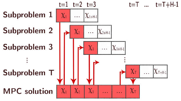
In this subsection, we briefly sketch out the implementation details of MPC. Even the convexified problem may be difficult to solve over long time horizons, i.e. when $T$ is large, since the number of decision variables scales as $O(T)$. MPC posits that (14) may be approximately solved by dividing it into $T$ sub-problems, with the $t^{\text{th}}$ subproblem defined over the variables $\{\mathcal{X}_{t},\cdots,\mathcal{X}_{t+H-1}\}$ and considering the relaxed constraints restricted to those involving the variables $\{\mathcal{X}_{t},\cdots,\mathcal{X}_{t+H-1}\}$. Since $\mathcal{X}_{t-1}$ is not a decision variable in the $t^{\text{th}}$ subproblem, its value is fixed as the optimal value of $\mathcal{X}_{t-1}$ derived from the $(t-1)^{\text{th}}$ subproblem. Thus, MPC allows for a solution of (14) by solving $T$ subproblems over time horizons of size $H$, instead of one problem over a time horizon of size $T$. The scheme is represented visually in Figure 1. Note that choosing $H=T$ and considering only the first subproblem reduces to solving the relaxed instance of (14) in a one-shot fashion.

4 Solution using Constrained Policy Optimization

Figure 2: Schematic of RL framework to solve load restoration.

We motivate the use of CPO to solve (14) by considering whether the decision variables and available information for the $t^{\text{th}}$ MPC subproblem (which starts at time $t$), denoted by $\mathbf{X}_{t}\stackrel{{\scriptstyle\Delta}}{{=}}\{\mathcal{X}_{t^{\prime}}\}_{t^{\prime}=t}^{t+H-1}\cup\mathcal{X}_{t-1}$ can be split into three groups, viz. state, action, and observation variables, such that they have the following properties:

• The state at time $t$, denoted by $\mathbf{x}_{t}$, represents the smallest set of variables in $\mathbf{X}_{t}$ plus exogenous data such as forecasts $\hat{P}^{\text{RES}}$, $\hat{P}^{\text{L}}$, and $\hat{Q}^{\text{L}}$, which can adequately describe the system at time $t$.

• The action at time $t$, denoted by $\mathbf{u}_{t}$, represents the set of variables in $\mathbf{X}_{t}$ which the MGC can control.

• The observation at time $t$, denoted by $\mathbf{o}_{t}$, denotes all variables in $\mathbf{X}_{t}\setminus\{\mathbf{u}_{t}\}$. Intuitively, the observation variables should be fully specified once $\mathbf{x}_{t}$ and $\mathbf{u}_{t}$ are known.

If such a split is possible, it allows for the introduction of a policy, which is a randomized map from a given state to a distribution over possible actions. Should we also define an objective function, which in the RL framework is called the reward, it becomes a well-posed problem to seek an optimal policy which maps state to actions in a way which maximizes the total accumulation of reward. Similar to MPC, each action is restricted to the subhorizon $\{t,\cdots,t+H-1\}$, and load restoration is done in a rolling-horizon fashion.

Armed with the motivation, we pose problem (14) as a constrained Markov decision process (CMDP) under the RL policy-learning framework of CPO. A CMDP is defined as the 6-tuple $\left\{\mathbb{X},\mathbb{U},p,R,\mathbf{{C}},\gamma\right\}$, where $\mathbb{X}$ is the state space, $\mathbb{U}$ is the action space, $p:\mathbb{X}\times\mathbb{U}\times\mathbb{X}\mapsto[0,1]$ is the state transition probability, $R:\mathbb{X}\times\mathbb{U}\mapsto\mathbb{R}$ is the reward function, $\mathbf{C}:\mathbb{X}\times\mathbb{U}\mapsto\mathbb{R}^{M}$ is the constraint function, and $\gamma\in(0,1]$ is the discount factor used to de-emphasize the contribution of uncertain future quantities to the reward. For many systems including the one under consideration, $p$, or the state transition probabilities is deterministic, based on known rules. The constraint function $\mathbf{C}$ is used to encode $M\geq 0$ constraints by representing them as $\mathbf{C}(\mathbf{x}_{t},\mathbf{u}_{t})\preceq\mathbf{0}$ on every time step $t$.

We now describe load restoration in the CPO framework by defining salient variables and functions. Then, we describe a tailored training process to find an optimal policy. Finally, we discuss the issue of evaluating various mathematical expressions which arise during the training process. We define the state $\mathbf{x}_{t}$ and the action $\mathbf{u}_{t}$ at time $t$ as:

$$\mathbf{x}_{t}\stackrel{{\scriptstyle\Delta}}{{=}} \bigg{\{}\left\{\mathcal{S}_{i,t-1}\right\}_{i\in\mathcal{N}^{\text{ESS}}},\left\{\zeta_{i,t-1}\right\}_{i\in\mathcal{N}^{\text{MT}}},\left\{\rho_{i,t-1}\right\}_{i\in\mathcal{N}^{\text{L}}},$$

$$\bigg{[}\left\{\hat{P}^{\text{L}}_{i,t^{\prime}},\hat{Q}^{\text{L}}_{i,t^{\prime}}\right\}_{i\in\mathcal{N}^{\text{L}}},\left\{\hat{P}^{\text{RES}}_{i,t^{\prime}}\right\}_{i\in\mathcal{N}^{\text{RES}}}\bigg{]}_{t^{\prime}=t}^{t+H-1}\bigg{\}}$$ (15)

$$\mathbf{u}_{t}\stackrel{{\scriptstyle\Delta}}{{=}} \bigg{\{}\bigg{[}\left\{s_{i,t^{\prime}}\right\}_{i\in\mathcal{N}^{\text{RES}}},\left\{s_{i,t^{\prime}}\right\}_{i\in\mathcal{N}^{\text{MT}}},\left\{\rho_{i,t^{\prime}}\right\}_{i\in\mathcal{N}^{\text{L}}}$$

$$\left\{P^{\text{ch}}_{i,t^{\prime}},P^{\text{dis}}_{i,t^{\prime}},\Im(s_{i,t^{\prime}})\right\}_{i\in\mathcal{N}^{\text{ESS}}}\bigg{]}_{t^{\prime}=t}^{t+H-1}\bigg{\}}.$$ (16)

The observation variables are simply defined as $\mathbf{o}_{t}\stackrel{{\scriptstyle\Delta}}{{=}}\mathbf{X}_{t}\setminus\{\mathbf{u}_{t}\}$. A policy $\pi_{\boldsymbol{\theta}}:\mathbb{X}\times\mathbb{U}\mapsto[0,1]$ parameterized by ${\boldsymbol{\theta}}\in\mathbb{R}^{h}$ (where $h$ is the number of elements in the parameter vector) and denoted as $\pi_{\boldsymbol{\theta}}(\mathbf{u}|\mathbf{x})$ gives the probability of taking action $\mathbf{u}$ given the current state $\mathbf{x}$. Usually, the policy maps from observation to action variables; however, we choose a fully observable setup wherein $\mathbf{x}_{t}$ contains variables from $\mathbf{o}_{t}$ as well as forecasts, and the policy mapping from state to action variables follows. A schematic of the evolution of state, action, and observation variables is shown in Figure 2. We model the policy as a multivariate Gaussian distribution whose mean vector and covariance matrix are generated by a feedforward neural network (FNN). This allows the policy to explore various possible trajectories during the process of training. To this end, let $d$ denote dimension of the action variable, and

$$\pi_{\boldsymbol{\theta}}(\mathbf{u}|\mathbf{x})=\frac{1}{\sqrt{|\boldsymbol{\Sigma}_{\mathbf{x}}|(2\pi)^{d}}}e^{-\frac{1}{2}(\mathbf{u}-\boldsymbol{\mu}_{\mathbf{x}})^{\top}\boldsymbol{\Sigma}_{\mathbf{x}}^{-1}(\mathbf{u}-\boldsymbol{\mu}_{\mathbf{x}})}\,,$$ (17)

where $\boldsymbol{\mu}_{\mathbf{x}}\in\mathbb{R}^{d}$ and $\boldsymbol{\Sigma}_{\mathbf{x}}\in\mathbb{R}^{d\times d}$ are generated by using an FNN denoted by $f_{\boldsymbol{\theta}}(\mathbf{x})$ as

$$\boldsymbol{\mu}_{\mathbf{x}}=L_{\boldsymbol{\mu}}(f_{\boldsymbol{\theta}}(\mathbf{x})),\quad\boldsymbol{\Sigma}_{\mathbf{x}}=M(L_{\boldsymbol{\Sigma}}(f_{\boldsymbol{\theta}}(\mathbf{x}))),$$ (18)

wherein $L_{\boldsymbol{\mu}}$ and $L_{\boldsymbol{\Sigma}}$ are linear functions which simply map some parts of the FNN output to the $d$-dimensional vector $\boldsymbol{\mu}_{\mathbf{x}}$, and other parts to the $d\times d$ dimensional matrix. In this case, ${\boldsymbol{\theta}}$ represents the weights and biases which describe the FNN. The function $M:d\times d\mapsto d\times d$, defined as $M(\mathbf{A})\stackrel{{\scriptstyle\Delta}}{{=}}\mathbf{A}\mathbf{A}^{\top}$ ensures that the matrix $\boldsymbol{\Sigma}_{\mathbf{x}}$ is always positive definite, which cannot otherwise be ensured for an arbitrary $d\times d$ matrix output from an FNN. For the rest of the paper, we refer to both policy distribution $\pi_{\boldsymbol{\theta}}$ and parameter vector ${\boldsymbol{\theta}}$ as ‘policy’, with the exact meaning evident from the context.

The design of the reward function is essentially the same as that of $J_{\mathcal{T}}$ in (1), except that it is defined over a shorter time horizon, and terms further in the future are discounted with the discount factor $\gamma$. The reward at time $t$ is given as:

$$R(\mathbf{x}_{t},\mathbf{u}_{t})=\textstyle\sum_{t^{\prime}=t}^{t+H} \gamma^{(t-t^{\prime})}\big{[}{\textstyle\sum_{i\in\mathcal{N}^{\text{L}}}C^{\text{L}}_{i,t^{\prime}}(\Re(s_{i,t^{\prime}}))}+$$

$${\textstyle\sum_{i\in\mathcal{N}^{\text{MT}}}C^{\text{MT}}_{i,t^{\prime}}(\Re(s_{i,t^{\prime}}))}\big{]}.$$

The constraints on the variables in action $\mathbf{u}_{t}$ is denoted by the vector-valued function $\mathbf{C}(\mathbf{x}_{t},\mathbf{u}_{t})\preceq\mathbf{0}$. Note that we consider only inequality constraints (‘$\leq$’) from load restoration in $\mathcal{J}^{C}$, while equality constraints are embedded implicitly in the observation generation procedure, which solves (14) with all the unspecified variables. This allows for a simulator-free implementation of CPO; indeed, (14) can itself be considered a ‘simulator’ for the current application. We define the reward function and constraint function at time $t$ as

$$\mathcal{J}^{R}(\pi_{\boldsymbol{\theta}},\mathbf{x}_{t}) \stackrel{{\scriptstyle\Delta}}{{=}}\mathbb{E}_{\mathbf{u}_{t}\sim\pi_{\boldsymbol{\theta}}}\left[R(\mathbf{x}_{t},\mathbf{u}_{t})\,|\,\mathbf{x}_{t}\right],$$

$$\mathcal{J}^{\mathbf{C}}(\pi_{\boldsymbol{\theta}},\mathbf{x}_{t}) \stackrel{{\scriptstyle\Delta}}{{=}}\mathbb{E}_{\mathbf{u}_{t}\sim\pi_{\boldsymbol{\theta}}}\left[\mathbf{C}(\mathbf{x}_{t},\mathbf{u}_{t})\,|\,\mathbf{x}_{t}\right].$$

Algorithm 1 Training load restoration policy with CPO

Input: Initial weights $\boldsymbol{\theta}$, number of episodes $E$, batch size $B$, Look-ahead window $H$, Multiple RES and load forecasts $\{\hat{P}^{\text{RES}}\},\{\hat{P}^{\text{L}}\}$
Output: Trained policy weights $\boldsymbol{\theta}$

1:for $e=1$ to $E$ do $\triangleright$ episodes

2:     Choose $P^{\text{RES}}$ and $P^{\text{L}}$ for current episodes

3:     for $t\in\mathcal{T}$ do $\triangleright$ time horizon

4:         Generate state $\mathbf{x}_{t-1}$ from $\mathbf{o}_{t-1}$, forecasts

5:         Sample $\mathcal{N}(\mathbf{0},\mathbf{I}^{\text{id}}_{d})$ $B$ times as $\{\boldsymbol{\epsilon}^{(b)}\}_{b\in[B]}$

6:         Generate coefficients $\mathbf{a}_{t},\mathbf{B}_{t},\mathbf{c}_{t}$, $\mathbf{F}_{t}$ using Proposition 1 and Lemma 4.3 $\triangleright$ exploration by policy

7:         if $\text{mod}(t,m)=0$ then $\triangleright$ FIM stale update

8:              Generate $\boldsymbol{\Sigma}^{-1}_{\boldsymbol{\theta}}$ using Prop 1 and Lemma 4.3

9:         end if

10:         Update $\boldsymbol{\theta}$ by solving (20)

11:     end for

12:end for

13:return $\boldsymbol{\theta}$

The load restoration problem can be solved by determining a policy ${\boldsymbol{\theta}}^{*}$ such that for any state $\mathbf{x}$, $\pi_{{\boldsymbol{\theta}}^{*}}$ maximizes $\mathcal{J}^{R}(\pi_{{\boldsymbol{\theta}}^{*}},\mathbf{x})$ while respecting the constraints $\mathcal{J}^{\mathbf{C}}(\pi_{{\boldsymbol{\theta}}^{*}},\mathbf{x})\preceq\mathbf{0}$. Since finding a ${\boldsymbol{\theta}}^{*}$ which produces the optimal action for all possible states is an intractable problem, we instead adopt the framework of training ${\boldsymbol{\theta}}$ episodically. Thus, a near-optimal policy ${\boldsymbol{\theta}}^{*}$ can be found in an episodic fashion by sequentially solving the following problem :

$${\boldsymbol{\theta}}_{t+1}=\operatorname*{arg\,max}\limits_{{\boldsymbol{\theta}}}\, \mathcal{J}^{R}(\pi_{\boldsymbol{\theta}},\mathbf{x}_{t})$$ (19a)

s.t. $$\mathcal{J}^{\mathbf{C}}(\pi_{\boldsymbol{\theta}},\mathbf{x}_{t})\preceq\mathbf{0}$$ (19b)

$$D_{\text{KL}}\left(\pi_{\boldsymbol{\theta}}(\,.\,|\mathbf{x}_{t})\lVert\pi_{{\boldsymbol{\theta}}_{t}}(\,.\,|\mathbf{x}_{t})\right)\leq\delta,$$ (19c)

where $\delta>0$ is the trust region parameter to ensure that successive policies do not have large variations. The final policy ${\boldsymbol{\theta}}^{*}$ is then determined as ${\boldsymbol{\theta}}^{*}=\lim\limits_{t\rightarrow\infty}{\boldsymbol{\theta}}_{t}$. Since the original problem (14) is only defined for $t\in\mathcal{T}$ and not for all $t\in\mathbb{N}$, we ‘loop back’ to a different initial state $\mathbf{x}_{0}$ at time $T+1$. This idea of training multiple times over $\mathcal{T}$ using different initial conditions is referred to as episodic training.

Directly solving (19) is challenging due to the highly nonlinear and non-convex optimization landscape of (19), which arises from to the nonlinearity of FNNs. In order to alleviate this challenge, we replace (19) with a quadratically constrained quadratic program (QCQP) approximation, which is well known in literature [21].

$${\boldsymbol{\theta}}_{t+1}=\operatorname*{arg\,max}_{{\boldsymbol{\theta}}}\, \mathbf{a}_{t}^{\top}({\boldsymbol{\theta}}-{\boldsymbol{\theta}}_{t})$$ (20a)

s.t. $$\mathbf{B}_{t}^{\top}({\boldsymbol{\theta}}-{\boldsymbol{\theta}}_{t})+\mathbf{c}_{t}\preceq\mathbf{0}$$ (20b)

$$({\boldsymbol{\theta}}-{\boldsymbol{\theta}}_{t})^{\top}\mathbf{F}_{t}({\boldsymbol{\theta}}-{\boldsymbol{\theta}}_{t})\leq\delta,$$ (20c)

The above QCQP approximation is obtained by replacing the objective function (19a) and constraint function (19b) with their first-order Taylor approximations (20a) and (20b) respectively. The KL Divergence constraint (19c) is replaced with its second-order Taylor approximation (20c), since its first-order approximation vanishes [33]. $\mathbf{F}_{t}$ is positive definite by construction [33], and therefore constraint (20c) is convex.

The challenge in adapting CPO to any given application is find an accurate and efficient algorithm for computing $\mathbf{a}_{t}$, $\mathbf{B}_{t}$, $\mathbf{c}_{t}$, and $\mathbf{F}_{t}$ on every time step $t$. In the following proposition, we present a procedure to generate said variables on every $t$, which simply requires an expectation over a standard normal variable, along with the partial derivative of the reward and constraint functions with respect to action. This is a significant improvement over the training procedure presented in [10] which requires multiple matrix inversions and matrix exponential evaluations per time step.

Proposition 1 (Parameters in problem (20)).

Define the variables $\boldsymbol{\mu}_{{\boldsymbol{\theta}}}\stackrel{{\scriptstyle\Delta}}{{=}}L_{\mathbf{\boldsymbol{\mu}}}(f_{\boldsymbol{\theta}}(\mathbf{x}_{t}))$ and $\boldsymbol{\Sigma}_{\boldsymbol{\theta}}\stackrel{{\scriptstyle\Delta}}{{=}}M(L_{\boldsymbol{\Sigma}}(f_{\boldsymbol{\theta}}(\mathbf{x}_{t})))$. Then, we have

$$\mathbf{a}_{t}=\left(\mathbb{E}_{\boldsymbol{\epsilon}\sim\mathcal{N}(\mathbf{0},\mathbf{I}^{\text{id}}_{d})}\left[\frac{\partial R_{t}}{\partial\mathbf{u}_{t}}\left((\boldsymbol{\epsilon}^{\top}\otimes\mathbf{I}^{\text{id}}_{d})\frac{\partial\mathbf{v}_{\boldsymbol{\theta}}}{\partial{\boldsymbol{\theta}}}+\frac{\partial\boldsymbol{\mu}_{\boldsymbol{\theta}}}{\partial{\boldsymbol{\theta}}}\right)\,\bigg{|}\,\mathbf{x}_{t}\right]\right)_{{\boldsymbol{\theta}}={\boldsymbol{\theta}}_{t}}$$

$$\mathbf{B}_{t}=\left(\mathbb{E}_{\boldsymbol{\epsilon}\sim\mathcal{N}(\mathbf{0},\mathbf{I}^{\text{id}}_{d})}\left[\frac{\partial\mathbf{C}_{t}}{\partial\mathbf{u}_{t}}\left((\boldsymbol{\epsilon}^{\top}\otimes\mathbf{I}^{\text{id}}_{d})\frac{\partial\mathbf{v}_{\boldsymbol{\theta}}}{\partial{\boldsymbol{\theta}}}+\frac{\partial\boldsymbol{\mu}_{\boldsymbol{\theta}}}{\partial{\boldsymbol{\theta}}}\right)\,\bigg{|}\,\mathbf{x}_{t}\right]\right)_{{\boldsymbol{\theta}}={\boldsymbol{\theta}}_{t}}$$

$$\mathbf{c}_{t}=J^{\mathbf{C}}(\pi_{{\boldsymbol{\theta}}_{t}},\mathbf{x}_{t})$$

$$\mathbf{F}_{t}(i,j)=\bigg{[}\frac{\partial\boldsymbol{\mu}_{\boldsymbol{\theta}}^{\top}}{\partial{\boldsymbol{\theta}}(i)}\boldsymbol{\Sigma}_{\boldsymbol{\theta}}^{-1}\frac{\partial\boldsymbol{\mu}_{\boldsymbol{\theta}}}{\partial{\boldsymbol{\theta}}(j)}+\frac{1}{2}\operatorname{Tr}\left(\boldsymbol{\Sigma}_{\boldsymbol{\theta}}^{-1}\frac{\partial\boldsymbol{\Sigma}_{\boldsymbol{\theta}}}{\partial{\boldsymbol{\theta}}(i)}\boldsymbol{\Sigma}_{\boldsymbol{\theta}}^{-1}\frac{\partial\boldsymbol{\Sigma}_{\boldsymbol{\theta}}}{\partial{\boldsymbol{\theta}}(j)}\right)\bigg{]}_{{\boldsymbol{\theta}}={\boldsymbol{\theta}}_{t}}$$

where $R_{t}\stackrel{{\scriptstyle\Delta}}{{=}}R(\mathbf{x}_{t},\mathbf{u}_{t})$, $\mathbf{C}_{t}\stackrel{{\scriptstyle\Delta}}{{=}}\mathbf{C}(\mathbf{x}_{t},\mathbf{u}_{t})$, $\mathbf{v}_{\boldsymbol{\theta}}\stackrel{{\scriptstyle\Delta}}{{=}}\text{vec}(\boldsymbol{\Sigma}_{\boldsymbol{\theta}})$, and $\mathbf{F}_{t}(i,j)$ and ${\boldsymbol{\theta}}(i)$ are the ${(i,j)}^{\text{th}}$ and ${i}^{\text{th}}$ element of $\mathbf{F}_{t}$ and ${\boldsymbol{\theta}}$, respectively.

Proof 4.1.

See Appendix .3.

In the following remark, we highlight some implementation details of the formulae presented in Proposition 1.

Remark 4.2 (Implementation of Proposition 1).

Firstly, we observe that in their definitions, $\mathbf{a}_{t}$ and $\mathbf{B}_{t}$ are defined in the form of an expectation over $\boldsymbol{\epsilon}\in\mathcal{N}(\mathbf{0},\mathbf{I}^{\text{id}}_{d})$, which would result in the linear term $\boldsymbol{\epsilon}^{\top}$ inside the expression being nullified. In practice, we implement the expectation through a sample average over samples of $\boldsymbol{\epsilon}$ which are produced by a random number generator, and since we don’t use infinite samples, the term $\boldsymbol{\epsilon}^{\top}$ is not nullified. Secondly, we note that evaluating $\mathbf{F}_{t}$ requires inverting the matrix $\boldsymbol{\Sigma}_{\boldsymbol{\theta}}^{-1}\in\mathbb{R}^{d\times d}$ on every time step. As a workaround, we implement stale updates, which means that $\boldsymbol{\Sigma}_{\boldsymbol{\theta}}^{-1}$ is updated only once every $m$ time steps. Thirdly, note that once $\mathbf{x}_{t}$ and $\mathbf{u}_{t}$ are known, the variables in $\mathbf{o}_{t}$ can be derived by solving an constraint satisfaction problem using the constraints of (14). This is equivalent to using (14) as an environment for the CPO agent in lieu of external simulators. $\blacksquare$

The partial derivatives of $\mathbf{v}_{\boldsymbol{\theta}}$, $\mathbf{u}_{\boldsymbol{\theta}}$, and $\boldsymbol{\Sigma}_{\boldsymbol{\theta}}$ in Proposition 1 with respect to ${\boldsymbol{\theta}}$ may be calculated via backpropagation operation [22, Algorithms 6.3 and 6.4] on the FNN, which is a standard operation for any software capable of handling FNNs. Now, it only remains to develop a procedure to evaluate $\frac{\partial R_{t}}{\partial\mathbf{u}_{t}}$ and $\frac{\partial\mathbf{C}_{t}}{\partial\mathbf{u}_{t}}$. The procedure we develop is unique to the DistFlow equations, and is similar for both the terms, and therefore we only demostrate the evaluation of $\frac{\partial R_{t}}{\partial\mathbf{u}_{t}}$.

For generic variables $a$ and $b$, let the expressions $a\in R_{t}$ and $b\in\mathbf{u}_{t}$ imply that $a$ makes an appearance in the closed form of $R_{t}$, and $b$ is a variable in $\mathbf{u}_{t}$. The evaluation of $\frac{\partial R_{t}}{\partial\mathbf{u}_{t}}$ therefore boils down to the efficient evaluation of $\frac{\partial a}{\partial b}$. To this end, we collect the equations which couple variables in $\mathbf{x}_{t}$, $\mathbf{u}_{t}$, and $\mathbf{o}_{t}$ over the time horizon $\{t,\cdots,t+H\}$, and evaluate their total differential as follows:

$$ds_{i,t}=\sum_{j\rightarrow k}dS_{jk,t}-\sum_{i\rightarrow j}(dS_{ij,t}-z_{ij}dl_{ij,t}),$$ (21a)

$$dv_{j,t}=dv_{i,t}-2\Re(\bar{z}_{ij}dS_{ij,t})+|z_{ij}|^{2}dl_{ij,t},$$ (21b)

$$dl_{ij,t}v_{i,t}+l_{ij,t}dv_{j,t}=2\Re(\bar{S}_{ij,t}dS_{ij,t}),$$ (21c)

$$P^{\text{dis}}_{i,t}dP^{\text{ch}}_{i,t}+dP^{\text{dis}}_{i,t}P^{\text{ch}}_{i,t}=0$$ (21d)

$$\Re(ds_{i,t})=dP^{\text{dis}}_{i,t}-dP^{\text{ch}}_{i,t},$$ (21e)

$$d\mathcal{S}_{i,t+1}=d\mathcal{S}_{i,t}+(\eta^{\text{ch}}_{i}\Delta_{t})dP^{\text{ch}}_{i,t}-\left(\frac{\Delta_{t}}{\eta^{\text{dis}}_{i}}\right)dP^{\text{dis}}_{i,t},$$ (21f)

$$d\varsigma_{i,t+1}=d\varsigma_{i,t}-\tau_{i}\Re(ds_{i,t}),$$ (21g)

$$\Re(ds_{i,t})=-d\rho_{i,t}\hat{P}^{\text{L}}_{i,t},\;\;\Im(ds_{i,t})=-d\rho_{i,t}\hat{Q}^{\text{L}}_{i,t}$$ (21h)

$$\Re(ds_{i,t})=-d\kappa_{i,t}\hat{P}^{\text{RES}}_{i,t},$$ (21i)

$$d\omega_{t}=-k_{P}\Re(ds_{i,t}),$$ (21j)

$$\left(\sqrt{v_{i,t}}\right)^{-1}dv_{i,t}=-2k_{Q}\Re(ds_{i,t}),$$ (21k)

where (21a) holds for all $j\in\mathcal{N}$, (21b)–(21c) hold for all $i\rightarrow j$, (21d)–(21f) hold for all $i\in\mathcal{N}^{\text{ESS}}$,(21g) holds for all $i\in\mathcal{N}^{\text{MT}}$, (21h) holds for all $i\in\mathcal{N}^{\text{L}}$, (21i) holds for all $i\in\mathcal{N}^{\text{RES}}$, and (21j)-(21k) hold for all $i\in\mathcal{N}^{\text{droop}}$. Note that (21) is a homogeneous system of linear equations in the differentials, which can be used to numerically calculate the required partial derivatives via the following result.

Lemma 4.3.

The partial derivative $\frac{\partial a}{\partial b}$ for $a\in R_{t}$ and $b\in\mathbf{u}_{t}$ may be evaluated by setting $db^{\prime}=0$ for all $b^{\prime}\in\mathbf{u}_{t}$ such that $b\neq b^{\prime}$, and solving (21) for $da$ and $db$. A solution exists if number of loads exceeds non-loads, in which case $\frac{\partial a}{\partial b}=\frac{da}{db}$.

Proof 4.4.

See Appendix .4.

All the steps involved in CPO training are summarized in Algorithm 1.

MG implementation

After we train the FNN for a large number of time steps $t$ in an episodic fashion, the trained FNN may be used as the MGC. If deterministic policies are desired then the mean $\boldsymbol{\mu}_{\mathbf{x}}$ may be used, while the covariance matrix $\boldsymbol{\Sigma}_{\mathbf{x}}$ may be nullified. On the other hand, if stochastic policies are desired, both $\boldsymbol{\mu}_{\mathbf{x}}$ and $\boldsymbol{\Sigma}_{\mathbf{x}}$ may be retained.

5 Simulation Results

Figure 3: A 36-bus MG that is adapted from the IEEE 37-bus distribution feeder.

(a)

(b)

(c)

(d)

(e)

(f)

Figure 4: Simulation results for the 36-bus MG.

(a)

(b)

(c)

Figure 5: Simulation results for the 141-bus MG.

Table 1: System Parameters.

System Parameter	Value
$T(hours)$	24
$(\underline{v}(\text{p.u.}),\bar{v}(\text{p.u.}))$	$(0.95\text{p.u.},1.05\text{p.u.})$
$(\underline{P}^{\text{MT}}(\text{kW}),\overline{P}^{\text{MT}}(\text{kW}),\tau(\text{kW}))$	$(0,250,0.9)$
$(E_{0},\underline{P}^{\text{MT}}_{\text{rd}}(\text{kW}),\bar{P}^{\text{MT}}_{\text{ru}}(\text{kW}))$	$(930,25,-30)$
$(\bar{P}^{\text{ch}}(\text{kW}),\bar{P}^{\text{dis}}(\text{kW}),\eta^{\text{ch}},\eta^{\text{dis}})$	$(25,25,0.9,0.9)$
$\underline{\mathcal{S}}(\text{kW}),\bar{\mathcal{S}}(\text{kW}),\mathcal{S}^{\text{init}}$	$(30,900,665)$
$(\bar{Q}^{\text{MT}}(\text{kVar}),\bar{Q}^{\text{ESS}}(\text{kVar}),\bar{Q}^{\text{RES}}(\text{kVar}))$	$(35,35,70)$

Table 2: CPO Parameters.

CPO Parameter	36-bus MG	141-bus MG
FNN $f_{\boldsymbol{\theta}}$ layer sizes	$(344,100,75,440)$	$(1403,500,250,1630)$
Activation Function	$\tanh$	$\tanh$
Trust region $\delta$	0.001	0.008
$\boldsymbol{\epsilon}$ samples per time step	$32$	$64$
Stale update param. $m$	5	5

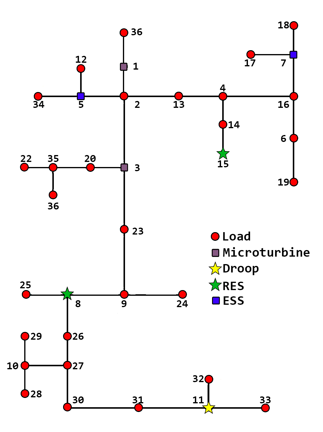
In this section, we use simulations to validate the performance of the proposed MPC and CPO approaches. In order to model the MG, we use a modified IEEE 37-bus test feeder [34], which prescribes network topology and power injection data. The 37-bus system is modified to a 36-bus system by deleting a bus interfaced with the network through a transformer, thereby maintaining same voltage upper and lower bounds across the MG. We also consider a MG based on a larger 141-bus radial feeder derived from case141 in MATPOWER [35].

All simulations were carried out in Python on a PC with an Intel Core i7 CPU, NVidia 1060Ti GPU, and 32GB of RAM. The Gurobi solver [36], interfaced with python through CVXPY [37], was used to find solutions for the MPC problem as well as solving (20). All FNN operations, as well as gradient calculations for Lemma 4.3 are calculated with PyTorch, and the automatic differentiation engine PyTorch Autograd.

We tested three algorithms which can solve (14) as follows:

• M1: This method uses a stochastic CPO policy trained according to (20a) for 1000 episodes for the 36-bus MG and 3000 episodes for the 141-bus MG. We use $H=5$ and $\gamma={0.8,0.9,1.0}$, and retain the value of $\gamma$ with the best performance. The parameters for the FNN used as the CPO policy, as well as other parameters involved in CPO, are displayed in Table 2. In order to relieve computational burden, we choose $\boldsymbol{\Sigma}_{\boldsymbol{\theta}}$ to be a diagonal matrix.

• M2: This method uses MPC to solve the proposed convex relaxation. We use $H=5$ and the convex relaxations proposed in Section 3.

• M3: We refer to this method as brute-force learning (BFL). It involves generating state-action pairs $(\mathbf{x}_{k},\mathbf{y}_{k})$, wherein the optimal actions are generated via M2. The data is generated for various renewable forecasts, similar to Algorithm 1. Then, we train a FNN on the input-output pairs. This method evaluates the performance of deep architectures which are trained in a supervised fashion, and are not privy to constraint-respecting training as in CPO.

36-bus MG

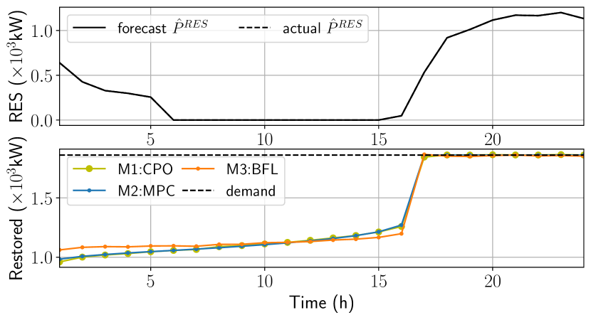
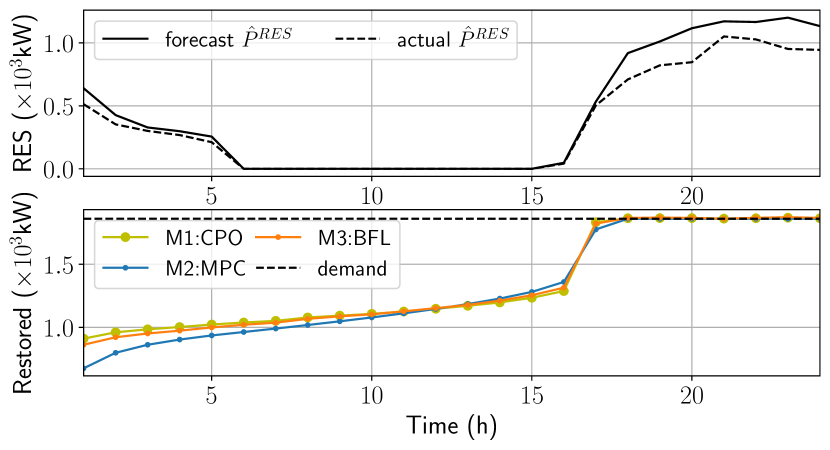
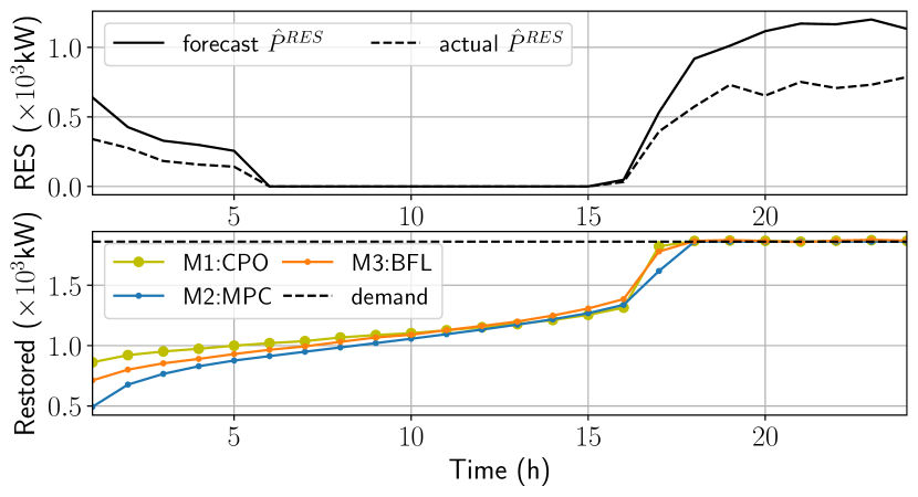
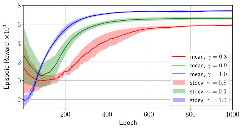
We first consider simulation results for the 36-bus MG. The parameters for various elements in the MG are listen in Table 1, and a one-line diagram of the MG is presented in Figure 3. We model the droop bus as an additional MT with similar parameters. The cost functions in (1) are chosen as $C^{\text{L}}_{i,t}(\Re(s_{i,t}))=-\Re(s_{i,t})$ (since load demands are negative) and $C^{\text{MT}}_{i,t}(\Re(s_{i,t}))=-0.75\Re(s_{i,t})$. The RES outputs are modeled as having a particular shape as shown in Figures 4(a)-4(c), and during training, they are perturbed uniformly by a factor of $[0.75,1.25]$ on each time step. The loads are chosen to be constant for the training in order to better demonstrate load restoration performance, and its values are derived from the case data.

The training curves for different values of $\gamma$ are presented in Figure 4(f). In the figure, the solid line shows the mean reward collected, while the shaded region indicates the variance of rewards over multiple training runs. In total, 500 training runs of Algorithm 1 were carried out and the best policy was used to generate final results and plots. From the figure, it can be seen that setting $\gamma=1$ leads to highest reward collection and also the lowest variance during training. Thus, $\gamma=1$ is used for the remaining experiments with the 36-bus MG. Next, we compare the load restoration process with uncertain values of $\hat{P}^{\text{RES}}$. In order to compare the load restoration performance of the three competing methods, we consider three scenarios as shown in Figures 4(a)-4(c). In the first scenario with perfect forecast, the performance of CPO is slightly worse than MPC and BFL, which demonstrates that under the availablity of perfect imformation, MPC solutions can be of higher quality than CPO. However, in scenarios where the actual RES output is lower than forecasts, as shown in Figures 4(b)-4(c), CPO shows better performance in terms of initial load pickup, as well as achieving full load restoration. This is due to the capability of CPO to learn from experience, and therefore during training it learns the best schedule for load restoration even under imperfect information. As opposed to this, MPC is restricted to only using forecast inputs for the current time step to $H$ time steps in the future, which poses a disadvantage in uncertain systems.

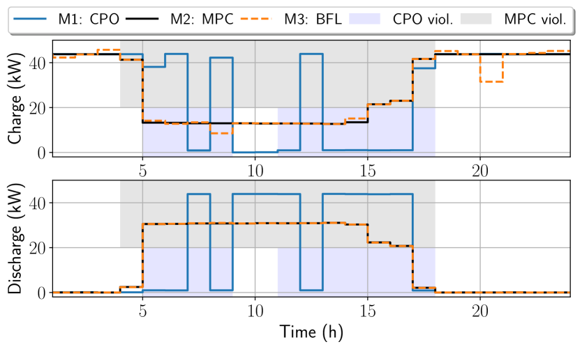
Next, we consider two relaxations proposed in Section 3. Figure 4(d) shows the charge and discharge performance for the ESS. Recall that for MPC, we use the relaxation proposed in Lemma 3.2, and the same is also inherited BFL suring its training. The gray shaded areas represent the time steps when MPC does not respect CC, while the blue shaded areas do the same for CPO. From here, it can be seen that CPO creates solution that adhere better to CC than CPO. Furthermore, even in the time steps when CPO violated CC, the magnitude of its violation is much lower than the solution produced by CPO and BFL. Therefore, we conclude that it is possible to implement the charge/discharge schedule produced by CPO directly to the MG, while MPC and BFL schedules require the post-hoc modification as discussed in Section 3.

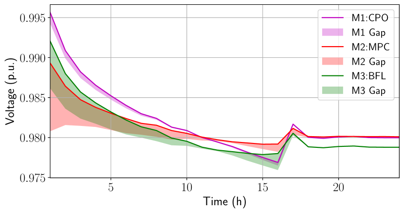
Finally, we consider the relaxation for voltage droop constraint presented in Lemma 1. It is possible to calculate the gap between the voltages derived as a result of the relaxed constraint, and the actual voltage of the unrelaxed constraint by evaluating (11c) using real power injections. From here, it can be seen that MPC and BFL incur large gaps between the relaxation and the actual voltages, especially in the initial time steps. This shows that the convex relaxation proposed in Lemma1 may not be tight in practice. However, the performance of CPO is much better in terms of the gap, thereby demonstrating that CPO is a better approach to satisfy the nonlinear droop constraints than relaxing them to a convex inequality constraint. However, further studies are required to establish conditions under which the proposed relaxation is tight, and holds exactly for all time steps.

141-bus MG

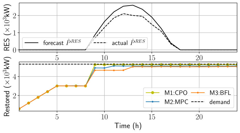
We now consider the simulation results for the 141-bus MG. The load demands are chosen from the case data, and multiple generation sources are incorporated into the MG. We place 7 MTs at buses $\{3,51,56,77,91,123,138\}$, 3 RESs at buses $\{12,43,88\}$, 6 ESS at buses $\{16,41,77,83,124,139\}$, and buses 56 and 91 operate under the principle of droop control. As in the 36-bus MG, the total load demands to be restored are constant and shown in Figure 5(a), while the RES forecast (with mispredictions) are also displayed in the same figure.

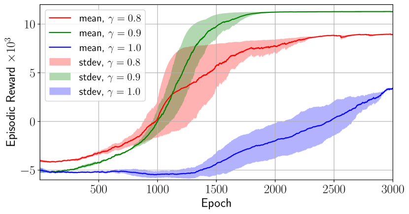
The training process of the CPO agent, as shown in Figure 5(b) shows that the best choice for parameter $\gamma$ is $\gamma=0.9$. Unlike the 36-bus MG, choosing $\gamma=1$ leads to a very unstable training trajectory, wherein the rewards remain low throughout training. Thus, we choose $\gamma=0.9$ for our experiments. The load restoration process under uncertain RES forecasts, as shown in Figure 5(a), shows that CPO performs slightly better than MPC and BFL, both in terms of load restored on any given time step, as well as reaching full load restoration. Furthermore, we compare the performance of CPO in satisfying the nonconvex DistFlow equation 2c. Recall that MPC and BFL use the relaxed second-order cone version of this constraint discussed in Section 3. In Figure 5(c), we calculate the gap resulting from this constraint not binding for all three methods. It can be seen that the gap for CPO is an order of magnitude lower in terms of maximum value than MPC or BFL. On the other hand, MPC and BFL enjoy zero gap on most buses, but an extremely high value of the gap on certain buses. Thus, the solutions produced these two methods enjoy lower exactness than the one produced by CPO.

Finally, we discuss the time taken for both training and online runtime for all three methods, which are presented in Table 3. The training time of CPO involves all steps presented in Algorithm 1, while the training time of BFL includes time taken for generation of data samples as well as training the FNN on these samples. While the training time for CPO is significantly longer than BFL, it also produces small runtimes. On the other hand, since CPO has to solve multiple optimization problems per time horizon, it results in the longest runtime. BFL has a smaller runtime than CPO due to a simpler FNN structure which does not take variance into account. From here, we see that CPO is competitive with respect to MPC in terms of runtime but this comes with a tradeoff of a far longer training time, which is absent in case of MPC.

Method	36-bus MG time		141-bus MG time
	Training	Runtime	Training	Runtime
CPO	4310s	0.51s	33780s	0.76s
MPC	-	2.76s	-	7.59s
BFL	345s	0.38s	1215s	0.62s

Table 3: Time taken by all three methods.

6 Conclusion

In this paper we considered the load restoration problem for an islanded MG, which contains sources of distributed power generation such as RES and MTs, as well as sources of energy storage, such as ESS. Two approaches to find a solution to the problem which can be implemented in the MGC were studied. We considered MPC, and proposed a convex relaxation of the load restoration problem which can be efficiently solved. We also developed CPO that finds an optimal policy through episodic training. Then, we compared the performance of MPC and CPO on 36-bus and 141-bus MGs. An important direction of future extension is to consider topology-switching MGs with discrete decision variables, and implement policies for the same using CPO. Other directions of investigation involve reducing of CPO training time through more efficient training strategies, and modeling of power sharing strategies in highly unbalanced multiphase MGs.

.1 Proof of Lemma 3.2

We will demonstrate that the provided second-order cone can be derived from the equation $\sqrt{v_{i,t}}=\sqrt{v_{i}^{*}}-k_{Q}(\Im(s_{i,t})-Q_{i}^{*})$ through a sequence of relaxations. We denote relaxations through the $\stackrel{{\scriptstyle\text{relax}}}{{\rightarrow}}$ symbol.

$$\sqrt{v_{i,t}}=\sqrt{v_{i}^{*}}-k_{Q}(\Im(s_{i,t})-Q_{i}^{*})$$

$$\stackrel{{\scriptstyle\text{relax}}}{{\rightarrow}}\; v_{i,t}=\left(\sqrt{v_{i}^{*}}-k_{Q}(\Im(s_{i,t})-Q_{i}^{*})\right)^{2}$$

$$\therefore\; \left(v_{i,t}\right)^{2}+v_{i,t}+\frac{1}{4}=\left(\sqrt{v_{i}^{*}}-k_{Q}(\Im(s_{i,t})-Q_{i}^{*})\right)^{2}+$$

$$\hskip 90.3375pt\left(v_{i,t}\right)^{2}+\frac{1}{4}$$

$$\therefore\; \left(v_{i,t}+\frac{1}{2}\right)^{2}=\left\lVert\begin{bmatrix}\sqrt{v_{i}^{*}}-k_{Q}(\Im(s_{i,t})-Q_{i}^{*})&v_{i,t}&\frac{1}{2}\end{bmatrix}\right\rVert_{2}^{2}$$

$$\therefore\; v_{i,t}+\frac{1}{2}=\left\lVert\begin{bmatrix}\sqrt{v_{i}^{*}}-k_{Q}(\Im(s_{i,t})-Q_{i}^{*})&v_{i,t}&\frac{1}{2}\end{bmatrix}\right\rVert_{2}$$

$$\stackrel{{\scriptstyle\text{relax}}}{{\rightarrow}}\; v_{i,t}+\frac{1}{2}\geq\left\lVert\begin{bmatrix}\sqrt{v_{i}^{*}}-k_{Q}(\Im(s_{i,t})-Q_{i}^{*})&v_{i,t}&\frac{1}{2}\end{bmatrix}\right\rVert_{2}.$$

.2 Proof of Lemma 1

Note that the points $(0,0)$, $(0,\bar{P}^{\text{dis}}_{i})$, and $(\bar{P}_{i}^{\text{ch}},0)$ are contained in $\mathcal{P}_{i}$, and therefore any convex set which contains $\mathcal{P}_{i}$ should contain $\operatorname{conv}\left\{(0,0),(0,\bar{P}_{i}^{\text{dis}}),(\bar{P}^{\text{ch}}_{i},0)\right\}$, which is exactly $\mathcal{P}^{\text{conv}}_{i}$. Thus, $\mathcal{P}^{\text{conv}}_{i}\subseteq\operatorname{conv}(\mathcal{P}_{i})$. On the other hand, $\mathcal{P}_{i}^{\text{conv}}$ is convex and contains the set $\mathcal{P}_{i}$, and therefore $\operatorname{conv}(\mathcal{P}_{i})\subseteq\mathcal{P}^{\text{conv}}_{i}$. It follows that $\operatorname{conv}(\mathcal{P}_{i})=\mathcal{P}^{\text{conv}}_{i}$.

.3 Proof of Theorem 1

The main idea of the proof is to replace the reward function, constraint function, and KL-divergence terms in (19) with their respective Taylor-series approximations around ${\boldsymbol{\theta}}_{t}$. The first-order approximation of the objective function is given as

$$\mathcal{J}^{R}(\pi_{\boldsymbol{\theta}},\mathbf{x}_{t})\approx\mathcal{J}^{R}(\pi_{{\boldsymbol{\theta}}_{t}},\mathbf{x}_{t})+\nabla_{{\boldsymbol{\theta}}}\mathcal{J}^{R}(\pi_{\boldsymbol{\theta}},\mathbf{x}_{t})\big{|}_{{\boldsymbol{\theta}}={\boldsymbol{\theta}}_{t}}({\boldsymbol{\theta}}-{\boldsymbol{\theta}}_{t}),$$

and by comparing the above approximation with (20), we see that $\mathbf{a}_{t}^{\top}=\nabla_{{\boldsymbol{\theta}}}\mathcal{J}^{R}(\pi_{\boldsymbol{\theta}},\mathbf{x}_{t})\big{|}_{{\boldsymbol{\theta}}={\boldsymbol{\theta}}_{t}}$. In order to compute $\mathbf{a}_{t}$, we need a closed-form of the gradient

$$\nabla_{\boldsymbol{\theta}}\mathcal{J}^{R}(\pi_{\boldsymbol{\theta}},\mathbf{x}_{t})=\nabla_{{\boldsymbol{\theta}}}\mathbb{E}_{\mathbf{u}_{t}\sim\pi_{{\boldsymbol{\theta}}}}\left[R(\mathbf{x}_{t},\mathbf{u}_{t})\,\big{|}\,\mathbf{x}_{t}\right],$$

which is difficult to evaluate since the gradient is with respect to ${\boldsymbol{\theta}}$ which parameterizes the distribution over which the expectation is being taken. To alleviate this difficulty, we use the reparametrization trick. For a standard normal vector $\boldsymbol{\epsilon}\sim\mathcal{N}(\mathbf{0},\mathbf{I}^{\text{id}}_{d})$, it holds that

$$\boldsymbol{\Sigma}_{\boldsymbol{\theta}}\boldsymbol{\epsilon}+\boldsymbol{\mu}_{\boldsymbol{\theta}}\sim\mathcal{N}(\boldsymbol{\mu}_{\boldsymbol{\theta}},\boldsymbol{\Sigma}_{\boldsymbol{\theta}}\boldsymbol{\Sigma}_{\boldsymbol{\theta}}^{\top}).$$

Therefore, letting $\mathbf{u}_{t}=\boldsymbol{\Sigma}_{\boldsymbol{\theta}}\boldsymbol{\epsilon}+\boldsymbol{\mu}_{\boldsymbol{\theta}}$ is equivalent to defining $\mathbf{u}_{t}$ as a Gaussian random vector with mean and variance given in (18). Thus, we have

$$\nabla_{\boldsymbol{\theta}}\mathbb{E}_{\mathbf{u}_{t}\sim\pi_{\boldsymbol{\theta}}}\left[R(\mathbf{x}_{t},\mathbf{u}_{t})\,\big{|}\,\mathbf{x}_{t}\right]$$

$$\hskip 10.84006pt=\nabla_{\boldsymbol{\theta}}\mathbb{E}_{\boldsymbol{\epsilon}\sim\mathcal{N}(\mathbf{0},\mathbf{I}^{\text{id}}_{d})}\left[R(\mathbf{x}_{t},\boldsymbol{\Sigma}_{\boldsymbol{\theta}}\boldsymbol{\epsilon}+\boldsymbol{\mu}_{\boldsymbol{\theta}})\,\big{|}\,\mathbf{x}_{t}\right]$$

$$\hskip 10.84006pt=\mathbb{E}_{\boldsymbol{\epsilon}\sim\mathcal{N}(\mathbf{0},\mathbf{I}^{\text{id}}_{d})}\left[\nabla_{\boldsymbol{\theta}}R(\mathbf{x}_{t},\boldsymbol{\Sigma}_{\boldsymbol{\theta}}\boldsymbol{\epsilon}+\boldsymbol{\mu}_{\boldsymbol{\theta}})\,\big{|}\,\mathbf{x}_{t}\right]$$

$$\hskip 10.84006pt=\mathbb{E}_{\boldsymbol{\epsilon}\sim\mathcal{N}(\mathbf{0},\mathbf{I}^{\text{id}}_{d})}\left[\frac{\partial R_{t}}{\partial\mathbf{u}_{t}}\frac{\partial\mathbf{u}_{t}}{\partial\boldsymbol{\Sigma}_{\boldsymbol{\theta}}}\frac{\partial\boldsymbol{\Sigma}_{\boldsymbol{\theta}}}{\partial{\boldsymbol{\theta}}}+\frac{\partial R_{t}}{\partial\mathbf{u}_{t}}\frac{\partial\mathbf{u}_{t}}{\partial\boldsymbol{\mu}_{\boldsymbol{\theta}}}\frac{\partial\boldsymbol{\mu}_{\boldsymbol{\theta}}}{\partial{\boldsymbol{\theta}}}\,\bigg{|}\,\mathbf{x}_{t}\right].$$ (22)

Computing $\frac{\partial\mathbf{u}_{t}}{\partial\boldsymbol{\Sigma}_{\boldsymbol{\theta}}}\frac{\partial\boldsymbol{\Sigma}_{\boldsymbol{\theta}}}{\partial{\boldsymbol{\theta}}}$ involves a multiplication of two tensors, which can be bypassed by vectorizing $\boldsymbol{\Sigma}_{\boldsymbol{\theta}}$. It follows that

$$\frac{\partial\mathbf{u}_{t}}{\partial\boldsymbol{\Sigma}_{\boldsymbol{\theta}}}\frac{\partial\boldsymbol{\Sigma}_{\boldsymbol{\theta}}}{\partial{\boldsymbol{\theta}}}=\frac{\partial\mathbf{u}_{t}}{\partial\mathbf{v}_{\boldsymbol{\theta}}}\frac{\partial\mathbf{v}_{\boldsymbol{\theta}}}{\partial{\boldsymbol{\theta}}}=\left(\boldsymbol{\epsilon}^{\top}\otimes\mathbf{I}^{\text{id}}_{d}\right)\frac{\partial\mathbf{v}_{\boldsymbol{\theta}}}{\partial{\boldsymbol{\theta}}}.$$

On the other hand, $\frac{\partial\mathbf{u}_{t}}{\partial\boldsymbol{\mu}_{\boldsymbol{\theta}}}\frac{\partial\boldsymbol{\mu}_{\boldsymbol{\theta}}}{\partial{\boldsymbol{\theta}}}=\frac{\partial\boldsymbol{\mu}_{\boldsymbol{\theta}}}{\partial{\boldsymbol{\theta}}}\times\frac{\partial\boldsymbol{\Sigma}_{\boldsymbol{\theta}}\boldsymbol{\epsilon}+\boldsymbol{\mu}_{\boldsymbol{\theta}}}{\partial\boldsymbol{\mu}_{\boldsymbol{\theta}}}=\frac{\partial\boldsymbol{\mu}_{\boldsymbol{\theta}}}{\partial{\boldsymbol{\theta}}}$. This verifies the closed form of $\mathbf{a}_{t}$ given in the theorem. The closed form of $\mathbf{B}_{t}$ can be similarly derived by computing the Jacobian of $\mathcal{J}^{\mathbf{C}}(\pi_{\boldsymbol{\theta}},\mathbf{x}_{t})$ at ${\boldsymbol{\theta}}={\boldsymbol{\theta}}_{t}$ (with $\mathbf{c}_{t}$ simply being the zeroth-order term in the Taylor expansion), carrying out the reparametrization trick and then deriving the closed form of the partial derivatives.

The first-order term in the Taylor approximation of constraint (19c) vanishes, and the second order term is used in the relaxed constraint (20c). Matrix $\mathbf{F}_{t}$ is the Fisher information matrix (FIM) that is positive semidefinite by construction. As provided in the theorem statement, the closed form of FIM for a Gaussian vector is well-known; see e.g., [33].

.4 Proof of Lemma 4.3

The numerical result proposed in the Lemma arises from the following observation.

Remark .1 (Evaluating partias from total derivatives).

For a generic problem, let the independent variable $\mathbf{p}$ and dependent variable $\mathbf{q}$ be related through the implicit equation $\mathbf{F}(\mathbf{p},\mathbf{q})=\mathbf{0}$, where $\mathbf{F}$ is a smooth function. The total differential of $\mathbf{F}(\mathbf{p},\mathbf{q})=\mathbf{0}$ is given as

$$\left[\frac{\partial\mathbf{F}(\mathbf{p},\mathbf{q})}{\partial\mathbf{p}}\right]^{\top}d\mathbf{p}+\left[\frac{\partial\mathbf{F}(\mathbf{p},\mathbf{q})}{\partial\mathbf{q}}\right]^{\top}d\mathbf{q}=\mathbf{0}.$$ (23)

To calculate $\frac{\partial p_{i}}{\partial q_{j}}$, we set $dp_{g}=0$ for all $g\neq j$ (a partial derivative with respect to $p_{j}$ means that any variables $p_{g}$ with $g\neq j$ are assumed to be constant), and solve (23) for $dp_{j}$ and $d\mathbf{q}$. From here, we have $\frac{\partial q_{i}}{\partial p_{j}}=\frac{dq_{i}}{dp_{j}}$.

Now, we show that the system of equations (21) always admits a solution when all action variables in $\mathbf{u}_{t}$ except one is nullified. We consider the real and imaginary parts of any complex differential equivalent to two real independent differentials. First, we calculate the number of linearly independent equations in (21). In order to detect linear dependencies, we note that equations among (21d)-(21k) which only contain a single term of the form $\Re(ds_{i,j})$ or $\Im(ds_{i,j})$ may be combined into (21a). Using this observation, we note that (21e), and (21g)-(21k) are linearly dependent on (21a). The total number of linearly independent equations, denoted by $N^{\text{eqn}}$, is therefore given as

$$N^{\text{eqn}}=H\left(2|\mathcal{N}|+2|\mathcal{E}|+2|\mathcal{N}^{\text{ESS}}|+2|\mathcal{N}^{\text{droop}}|\right).$$

On the other hand, the number of variables in $\mathbf{u}_{t}$ is given as

$$N^{\text{action}}=H\left(2|\mathcal{N}^{\text{MT}}|+2|\mathcal{N}^{\text{RES}}|+3|\mathcal{N}^{\text{ESS}}|+|\mathcal{N}^{\text{L}}|\right),$$

while the total number of variables in (21) is given as

$$N^{\text{vars}}=H\big{(} 3|\mathcal{N}|+3|\mathcal{E}|+3|\mathcal{N}^{\text{ESS}}|+|\mathcal{N}^{\text{MT}}|$$

$$+|\mathcal{N}^{\text{RES}}|+|\mathcal{N}^{\text{L}}|+1\big{)}.$$

From the above, it can be verified that $\big{(}N^{\text{vars}}-N^{\text{action}}+1\big{)}-N^{\text{eqns}}>0$ when $|\mathcal{N}|^{\text{L}}\geq|\mathcal{N}|^{\text{MT}}+|\mathcal{N}|^{\text{RES}}+|\mathcal{N}|^{\text{ESS}}$. Thus, the system of equations (21) when all but one action variable differentials are nullified, is a strictly underdetermined system of homogenous equations. Thus, it has a non-empty nullspace, and therefore a solution always exists.

References

- [1] H. Nazaripouya, “Power grid resilience under wildfire: A review on challenges and solutions,” in Proceedings of the 2020 IEEE Power Energy Society General Meeting, 2020, pp. 1–5.
- [2] M. Panteli and P. Mancarella, “Modeling and evaluating the resilience of critical electrical power infrastructure to extreme weather events,” IEEE Systems Journal, vol. 11, no. 3, pp. 1733–1742, 2017.
- [3] S. Moayedi and A. Davoudi, “Distributed tertiary control of dc microgrid clusters,” IEEE Transactions on Power Electronics, vol. 31, no. 2, pp. 1717–1733, 2016.
- [4] “IEEE standard for the specification of microgrid controllers,” IEEE Std 2030.7-2017, pp. 1–43, 2018.
- [5] A. G. Tsikalakis and N. D. Hatziargyriou, “Centralized control for optimizing microgrids operation,” in 2011 IEEE Power and Energy Society General Meeting, 2011, pp. 1–8.
- [6] W. A. Bukhsh, A. Grothey, K. I. M. McKinnon, and P. A. Trodden, “Local solutions of the optimal power flow problem,” IEEE Transactions on Power Systems, vol. 28, no. 4, pp. 4780–4788, 2013.
- [7] M. Farivar and S. H. Low, “Branch flow model: Relaxations and convexification—Part I,” IEEE Transactions on Power Systems, vol. 28, no. 3, pp. 2554–2564, 2013.
- [8] M. Baran and F. Wu, “Optimal capacitor placement on radial distribution systems,” IEEE Transactions on Power Delivery, vol. 4, no. 1, pp. 725–734, 1989.
- [9] A. Castillo and D. F. Gayme, “Grid-scale energy storage applications in renewable energy integration: A survey,” Energy Conversion and Management, vol. 87, pp. 885–894, 2014. [Online]. Available: https://www.sciencedirect.com/science/article/pii/S0196890414007018
- [10] Q. Zhang, K. Dehghanpour, Z. Wang, F. Qiu, and D. Zhao, “Multi-agent safe policy learning for power management of networked microgrids,” IEEE Transactions on Smart Grid, vol. 12, no. 2, pp. 1048–1062, 2021.
- [11] F. Shen, Q. Wu, J. Zhao, W. Wei, N. D. Hatziargyriou, and F. Liu, “Distributed risk-limiting load restoration in unbalanced distribution systems with networked microgrids,” IEEE Transactions on Smart Grid, vol. 11, no. 6, pp. 4574–4586, 2020.
- [12] K. Garifi, K. Baker, D. Christensen, and B. Touri, “Convex relaxation of grid-connected energy storage system models with complementarity constraints in dc opf,” IEEE Transactions on Smart Grid, vol. 11, no. 5, pp. 4070–4079, 2020.
- [13] N. Nguyen, S. Almasabi, A. Bera, and J. Mitra, “Optimal power flow incorporating frequency security constraint,” IEEE Transactions on Industry Applications, vol. 55, no. 6, pp. 6508–6516, 2019.
- [14] L. Jin, R. Kumar, and N. Elia, “Model predictive control-based real-time power system protection schemes,” IEEE Transactions on Power Systems, vol. 25, no. 2, pp. 988–998, 2010.
- [15] X. Zhang, G. Hug, J. Z. Kolter, and I. Harjunkoski, “Model predictive control of industrial loads and energy storage for demand response,” in Proceedings of the 2016 IEEE Power and Energy Society General Meeting, 2016, pp. 1–5.
- [16] S. C. Dhulipala, R. V. A. Monteiro, R. F. d. Silva Teixeira, C. Ruben, A. S. Bretas, and G. C. Guimarães, “Distributed model-predictive control strategy for distribution network Volt/VAR control: A smart-building-based approach,” IEEE Transactions on Industry Applications, vol. 55, no. 6, pp. 7041–7051, 2019.
- [17] T. Wang, H. Kamath, and S. Willard, “Control and optimization of grid-tied photovoltaic storage systems using model predictive control,” IEEE Transactions on Smart Grid, vol. 5, no. 2, pp. 1010–1017, 2014.
- [18] W. Wang, N. Yu, Y. Gao, and J. Shi, “Safe off-policy deep reinforcement learning algorithm for Volt-VAR control in power distribution systems,” IEEE Transactions on Smart Grid, vol. 11, no. 4, pp. 3008–3018, 2020.
- [19] H. Li, Z. Wan, and H. He, “Constrained EV charging scheduling based on safe deep reinforcement learning,” IEEE Transactions on Smart Grid, vol. 11, no. 3, pp. 2427–2439, 2020.
- [20] J. Duan, Z. Yi, D. Shi, C. Lin, X. Lu, and Z. Wang, “Reinforcement-learning-based optimal control of hybrid energy storage systems in hybrid AC–DC microgrids,” IEEE Transactions on Industrial Informatics, vol. 15, no. 9, pp. 5355–5364, 2019.
- [21] J. Achiam, D. Held, A. Tamar, and P. Abbeel, “Constrained policy optimization,” in Proceedings of the 34th International Conference on Machine Learning (ICML), 2017, pp. 22–31.
- [22] I. Goodfellow, Y. Bengio, and A. Courville, Deep Learning. MIT Press, 2016, http://www.deeplearningbook.org.
- [23] H. Li, Z. Wang, L. Li, and H. He, “Online microgrid energy management based on safe deep reinforcement learning,” in 2021 IEEE Symposium Series on Computational Intelligence (SSCI), 2021, pp. 1–8.
- [24] Y. Xu, C.-C. Liu, K. P. Schneider, F. K. Tuffner, and D. T. Ton, “Microgrids for service restoration to critical load in a resilient distribution system,” IEEE Transactions on Smart Grid, vol. 9, no. 1, pp. 426–437, 2018.
- [25] J. Li, X.-Y. Ma, C.-C. Liu, and K. P. Schneider, “Distribution system restoration with microgrids using spanning tree search,” IEEE Transactions on Power Systems, vol. 29, no. 6, pp. 3021–3029, 2014.
- [26] S. Ghasemi, M. Mohammadi, and J. Moshtagh, “A new look-ahead restoration of critical loads in the distribution networks during blackout with considering load curve of critical loads,” Electric Power Systems Research, vol. 191, p. 106873, 2021. [Online]. Available: https://www.sciencedirect.com/science/article/pii/S0378779620306714
- [27] X. Zhang, A. T. Eseye, B. Knueven, W. Liu, M. Reynolds, and W. Jones, “Curriculum-based reinforcement learning for distribution system critical load restoration,” IEEE Transactions on Power Systems, pp. 1–13, 2022.
- [28] S. Ghasemi and J. Moshtagh, “Distribution system restoration after extreme events considering distributed generators and static energy storage systems with mobile energy storage systems dispatch in transportation systems,” Applied Energy, vol. 310, p. 118507, 2022. [Online]. Available: https://www.sciencedirect.com/science/article/pii/S0306261921017220
- [29] L. W. Chung, M. Siam, A. Ismail, and Z. Hussien, “Modeling and simulation of sodium sulfur battery for battery-energy storage system and custom power devices,” in PECon 2004. Proceedings. National Power and Energy Conference, 2004., 2004, pp. 205–210.
- [30] J. Lopes, C. Moreira, and A. Madureira, “Defining control strategies for microgrids islanded operation,” IEEE Transactions on Power Systems, vol. 21, no. 2, pp. 916–924, 2006.
- [31] J. Rawlings, “Tutorial overview of model predictive control,” IEEE Control Systems Magazine, vol. 20, no. 3, pp. 38–52, 2000.
- [32] N. Nazir and M. Almassalkhi, “Guaranteeing a physically realizable battery dispatch without charge-discharge complementarity constraints,” IEEE Transactions on Smart Grid, pp. 1–1, 2021.
- [33] O. Besson and Y. I. Abramovich, “On the fisher information matrix for multivariate elliptically contoured distributions,” IEEE Signal Processing Letters, vol. 20, no. 11, pp. 1130–1133, 2013.
- [34] “Ieee 37-bus feeder,” https://cmte.ieee.org/pes-testfeeders/resources/, accessed: 2022-07-05.
- [35] R. D. Zimmerman, C. E. Murillo-Sánchez, and R. J. Thomas, “Matpower: Steady-state operations, planning, and analysis tools for power systems research and education,” IEEE Transactions on Power Systems, vol. 26, no. 1, pp. 12–19, 2011.
- [36] Gurobi Optimization, LLC, “Gurobi Optimizer Reference Manual,” 2022. [Online]. Available: https://www.gurobi.com
- [37] M. Grant and S. Boyd, “CVX: Matlab software for disciplined convex programming, version 2.1,” http://cvxr.com/cvx, Mar. 2014.