Fair-SSL: Building fair ML Software with less data

Abstract.

Ethical bias in machine learning models has become a matter of concern in the software engineering community. Most of the prior software engineering works concentrated on finding ethical bias in models rather than fixing it. After finding bias, the next step is mitigation. Prior researchers mainly tried to use supervised approaches to achieve fairness. However, in the real world, getting data with trustworthy ground truth is challenging and also ground truth can contain human bias.

Semi-supervised learning is a technique where, incrementally, labeled data is used to generate pseudo-labels for the rest of data (and then all that data is used for model training). In this work, we apply four popular semi-supervised techniques as pseudo-labelers to create fair classification models. Our framework, Fair-SSL, takes a very small amount (10%) of labeled data as input and generates pseudo-labels for the unlabeled data. We then synthetically generate new data points to balance the training data based on class and protected attribute as proposed by Chakraborty et al. in FSE 2021. Finally, classification model is trained on the balanced pseudo-labeled data and validated on test data. After experimenting on ten datasets and three learners, we find that Fair-SSL achieves similar performance as three state-of-the-art bias mitigation algorithms. That said, the clear advantage of Fair-SSL is that it requires only 10% of the labeled training data.

To the best of our knowledge, this is the first SE work where semi-supervised techniques are used to fight against ethical bias in SE ML models. To facilitate open science and replication, all our source code and datasets are publicly available at https://github.com/joymallyac/FairSSL.

1. Introduction

Machine learning software has become ubiquitous in our society. Software is making autonomous decisions in criminal sentencing (Tolan et al., 2019), loan approvals (for, 2011), patient diagnosis (Med, 2018), hiring candidates (hir, 2020), and whatnot. It is the duty of software researchers and engineers to produce high-quality software that always makes fair decisions. However, in recent times, there are numerous examples where machine learning software is found to have biased behavior based on some protected attributes like sex, race, age, marital status, etc. Google translate, the most popular translation engine in the world, shows gender bias. “She is an engineer, He is a nurse” is translated into Turkish and then again into English becomes “He is an engineer, She is a nurse” (Caliskan et al., 2017). YouTube makes more mistakes when it automatically generates closed captions for videos with female than male voices (Tatman, 2017). Amazon’s automated recruiting tool was found to be biased against women (Ama, 2018). A widely used face recognition software was found to be biased against dark-skinned women (Ski, 2018). Angel et al. commented that software showing bias is considered as poor quality software and should not be used in real life applications (Angell et al., [n.d.]). It is time for software engineering researchers to dive into the field of software fairness and try to build fairer software to prevent discriminative behaviors.

Table 1. Details of the datasets used in this research.

Dataset	#Rows	#Cols	Protected Attribute		Class Label
			Privileged	Unprivileged	Favorable	Unfavorable
Adult Census (ADU, 1994)	48,842	14	Sex-Male; Race-White	Sex-Female; Race-Non-white	High Income	Low Income
Compas (COM, 2015)	7,214	28	Sex-Male; Race-Caucasian	Sex-Female; Race-Not Caucasian	Did not reoffend	Reoffended
German Credit (GER, 2000)	1,000	20	Sex-Male	Sex-Female	Good Credit	Bad Credit
Default Credit (DEF, 2016)	30,000	23	Sex-Male	Sex-Female	Default Payment-Yes	Default Payment-No
Heart Health (HEA, 2001)	297	14	Age-Young	Age-Old	Not Disease	Disease
Bank Marketing (BAN, 2017)	45,211	16	Age-Old	Age-Young	Term Deposit - Yes	Term Deposit - No
Home Credit (HOM, 2017)	3,075,11	240	Sex-Male	Sex-Female	Approved	Rejected
Student Performance (STU, 2014)	1,044	33	Sex-Male	Sex-Female	Good Grade	Bad Grade
MEPS15 (MEP, 2015)	35,428	1,831	Race-White	Race-Non-white	Good Utilization	Bad Utilization
MEPS 16 (MEP, 2016)	34,656	1,941	Race-White	Race-Non-white	Good Utilization	Bad Utilization

Table 2. Definition of the performance and fairness metrics used in this study.

Performance Metric	Ideal Value	Fairness Metric	Ideal Value
Recall = TP/P = TP/(TP+FN)	1	Average Odds Difference (AOD): Average of difference in False Positive Rates(FPR) and True Positive Rates(TPR) for unprivileged and privileged groups TPR = TP/(TP + FN), FPR = FP/(FP + TN), AOD = [(FPR_U - FPR_P) + (TPR_U - TPR_P)] * 0.5	0
False alarm = FP/N = FP/(FP+TN)	0	Equal Opportunity Difference (EOD): Difference of True Positive Rates(TPR) for unprivileged and privileged groups. EOD = TPR_U - TPR_P	0
Accuracy = $\frac{(TP+TN)}{(TP+FP+TN+FN)}$	1	Statistical Parity Difference (SPD): Difference between probability of unprivileged group (PA = 0) gets favorable prediction ($\hat{Y}=1$) & probability of privileged group (PA = 1) gets favorable prediction ($\hat{Y}=1$). $SPD=P[\hat{Y}=1|PA=0]-P[\hat{Y}=1|PA=1]$	0
Precision = TP/(TP+FP)	1	Disparate Impact (DI): Similar to SPD but instead of the difference of probabilities, the ratio is measured. $DI=P[\hat{Y}=1|PA=0]/P[\hat{Y}=1|PA=1]$	1
F1 Score = $\frac{2*(Precision*Recall)}{(Precision+Recall)}$	1

A machine learning software can acquire bias in various ways (Brun and Meliou, 2018). Prior studies  (Jiang and Nachum, 2019; Chen et al., 2018) mentioned that most of the time bias comes from the training data. If training data contains improper labels, that bias gets induced into model while training. In an ACM SIGSOFT Distinguished award winning paper, Chakraborty et al. (Chakraborty et al., 2021) found out that bias comes from improper data labels and imbalanced data distribution. They said if the training data contains more examples of a certain group getting privileged (males being hired for a job) and another group getting betrayed (females getting more rejections); the machine learning model acquires that bias while training and in the future makes unfair predictions. Their algorithm, Fair-SMOTE, improved both the fairness and performance of the model and broke the premise of Berk et al. (Berk et al., 2017) who claimed “It is impossible to achieve fairness and high performance simultaneously (except in trivial cases)”.

We consider Fair-SMOTE (Chakraborty et al., 2021) as our baseline method. It is a supervised approach and uses 100% training data labels. But gathering good quality labeled data is very challenging. Human labeling is an extremely costly process  (3ds, 2021; goo, 2021; Tu et al., 2020a; Tu and Menzies, 2021) and there is a high possibility of human bias getting injected into the training data (James Manyika and Presten, 2019; Xiang, 2019). That said, blindly trusting ground truth labels may induce bias in the machine learning model. Hence, it is timely to ask:

Can we reduce the labeling effort associated with building fair models?

In this work, we try to answer that question by using semi-supervised learning (Zhu, 2006) that works with a small amount of labeled data and a large amount of unlabeled data. We build a framework called Fair-Semi-Supervised-Learning (Fair-SSL) that uses four state-of-the-art semi-supervised techniques - self-training, label propagation, label spreading, & co-training. Fair-SSL is a pseudo-labeling framework. It learns from the combination of labeled & unlabeled data and then pseudo-labels the unlabeled data. Results show that Fair-SSL performs as good as three other state-of-the-art fairness algorithms (Chakraborty et al., 2020a, 2021; Calmon et al., 2017). That means even if available ground truth is corrupted or a very few labeled data points are available initially, fairness could still be achievable. Overall, this paper makes the following contributions:

• This is the first SE work using semi-supervised learning to generate fair classification models.

• Fair-SSL works with a very small amount of labeled training data (10%). Thus, we can avoid the costly process of data labeling. Hence, it is cost effective.

• We have shown a technique based on “situation testing” (USA, 2007) to create fairly labeled data without using any human intervention.

• We have given a comparative analysis of four popular semi-supervised algorithms in the context of software fairness.

• Our results show that semi-supervised algorithms can be used to generate fairer and better performing models.

2. Background

Software Fairness - Big software industries have started putting more and more importance on ethical issues of ML software. AI Fairness 360 (AIF, 2018) from IBM, Fairlearn (Fai, 2021) from Microsoft are great initiatives to attract bigger audience. The software academic community, in spite of having a delayed start, is taking initiatives to fight against this critical social bane. ICSE 2018 hosted Fairware (FAI, 2018); ASE 2019 organized EXPLAIN (EXP, 2019). The IEEE (Shahriari and Shahriari, 2017), the European Union (EU, 2018) recently published the ethical principles of AI. It is stated that every machine learning software must be fair when it is used in real-life applications. Thus, testing software for bias and mitigating bias have now become an unavoidable step in software life cycle.

Some popular fairness testing tools are THEMIS  (Angell et al., [n.d.]), Symbolic Generation (Aggarwal et al., 2019), AEQUITAS  (Udeshi et al., 2018), and white-box testing tool (Zhang et al., 2020a). In case of bias mitigation, we see very few works in SE venues. As per our knowledge, there are only two frameworks Fairway (Chakraborty et al., 2020a) and Fair-SMOTE (Chakraborty et al., 2021) that tried to mitigate bias in SE ML models. Both of them are supervised methods that require a lot of labeled training data. We, in this work, used semi-supervised approach and achieved similar or better performance using only 10% labeled training data.
Semi-supervised Learning - Supervised machine learning models, specially the deep learning models, require a huge amount of labeled data for training. Gathering good quality labeled training data is the most expensive part of ML pipeline (3ds, 2021; goo, 2021). For labeling purpose, usage of human beings is a very expensive process (3ds, 2021; goo, 2021). Even then, human bias may get injected into training data (James Manyika and Presten, 2019; Xiang, 2019).

Semi-supervised learning (SSL) can address all these issues. SSL requires a small amount of labeled data to begin with (Zhu, 2006), then using an incremental approach, unlabeled data is pseudo-labeled, and the combined data is used for model training. SSL has been used in various domains of software engineering such as defect prediction (Zhang et al., 2017), test case prioritization (Yu et al., 2019), static warning analysis (Tu and Menzies, 2021), software vulnerability prediction (Yu et al., 2019), and many more. To the best of our knowledge, this paper is the first SE work to try SSL in the context of fairness. Outside of SE, we found only one study by Zhang et al. (Zhang et al., 2020b) studying SSL and fairness. Whereas they experimented on only three datasets and used only self-training technique, we evaluated our results based on nine metrics, ten datasets, and three learners.
Fairness Terminology & Metrics - At first, we need to define some fairness related terms. Table 1 contains ten datasets used in this study. Most of the prior works (Calmon et al., 2017; Galhotra et al., 2017; Zhang et al., 2018; Kamiran et al., 2018; Chakraborty et al., [n.d.]; Chakraborty et al., 2020b) used one or two datasets whereas we used ten of them. All these datasets are binary classification datasets i.e. class labels have two values. A class label is called a favorable label if it gives an advantage to the receiver such as receiving a loan, being hired for a job. A protected attribute is an attribute that divides the whole population into two groups (privileged & unprivileged) that have differences in terms of receiving benefits. For example, in Home Credit dataset, based on “sex”, “male” is privileged and “female” is unprivileged. In the context of classification, the goal of fairness is giving similar treatment to privileged and unprivileged groups.

Table 2 contains the definitions of the five performance metrics and four fairness metrics used in this study. We chose these metrics because they were widely used in the literature (Chakraborty et al., 2020a; Biswas and Rajan, 2020; Chakraborty et al., [n.d.]; Hardt et al., 2016; Chakraborty et al., 2020b; Chakraborty et al., 2021). For recall, precision, accuracy, F1 & DI larger values are better; For false alarm, AOD, EOD, & SPD smaller values are better. For readability, while showing results we compute abs(1 - DI) so that all four fairness metrics are lower the better (0 means no bias).

3. Methodology

Fair-SSL contains three major steps: a) Select a small amount of labeled data (10%) in a way that initial labeling does not contain bias (see §3.1); b) Pseudo-label the unlabeled data using semi-supervised approaches (see §3.2); c) Balance the combined training data (labeled + pseudo labeled) based on protected attribute and class label (see §3.3). Finally, we train ML models on the generated balanced data and test on the test data. We use 80-20 train-test division and test set is used only for final score reporting.

3.1. Prepare the Fairly Labeled data

Our first task is preparing the initial fairly labeled set. All the datasets in Table 1 are already labeled. But are those labels fair? Can we just randomly pick one portion of that data as fairly labeled? How much labeled data is required to start with? We are going to find all the answers soon.

Prior studies (Chakraborty et al., 2021; Das and Donini, 2020; Jiang and Nachum, 2019; Simons, 2020) have experimented with the datasets of Table  1 and found out that more or less 10% data labels contain unfair decisions. That means if we randomly pick up some portion of the data, we may end up selecting some improperly labeled rows and training ML models on that corrupted data will introduce bias. Thus, at an early stage, we decided to re-label the data.

In literature, there are mainly two approaches for executing the labeling process. The first one is manual labeling/crowdsourcing. The second one is semi-supervised pseudo-labeling. At first, we tried to do crowdsourcing for labeling. Our attempt was not successful. The datasets we use in the fairness domain are not very easy to be labeled by common people. Most are financial datasets; Compas is a criminal sentencing dataset; Heart health is a medical dataset. Hence special expertise is needed to label these kinds of data. It was out of our scope to find that kind of experienced people. Also, this manual labeling is a super expensive process. Besides, there is possibility of human bias getting injected into data labels (James Manyika and Presten, 2019; Xiang, 2019). Therefore, we discarded the idea of manual labeling.
Situation Testing: Chakraborty et al. reported that in these datasets, around 10% of the labels are unfair labels (Chakraborty et al., 2021). Thus we could select only fairly labeled rows from the available data and treat the rest as unlabeled data. To achieve that, we used the concept of situation testing (Zhang et al., 2016b). It is a research technique used in the legal field (USA, 2007) where decision makers’ candid responses to applicant’s personal characteristics are captured and analyzed.

At first, we divide the data based on the protected attribute. Then, we train two different logistic regression models (any other simple statistical model can be used) on those two subgroups (“male” and “female”). Then for all the training data points, we check the predictions of these two models. For a particular data point, if the predictions of two models match with the ground truth label, we keep the data point with the same label as it was fairly labeled. If the model predictions contradict with each other or the ground truth, we discard the label and treat the data point as unlabeled.

After this situation testing phase, we get the fairly labeled set. But we do not use this whole set for training. We take a small portion (10%) of this set to start. This selection is not a random selection. The normal trend of semi-supervised learning is keeping the initial labeled data balanced based on class so that the semi-supervised model gets an opportunity to learn features from all the classes equally (Hyun et al., 2020; Li et al., 2011). In fairness, data balancing helps more if instead of just class, protected attributes are also balanced (Chen et al., 2018; Yan et al., 2020; Chakraborty et al., 2021). Therefore, we select data points in a way that the initial fairly labeled set has equal proportion of “favorable-privileged (FP)” (for “Adult” dataset - “high income” & “male” ), “favorable-unprivileged (FU)” (“high income” & “female” ), “unfavorable-privileged (UP)” (“low income” & “male” ), & “unfavorable-unprivileged (UU)” (“low income” & “female” ) samples. Figure 1 shows the block diagram of the combined process of situation testing and sampling that generates perfectly balanced initial fairly labeled set.

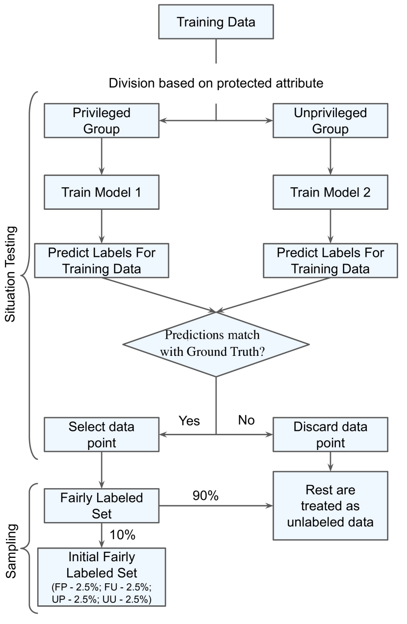
Figure 1. Algorithm for selecting/sampling fairly labeled data points from the available data.

3.2. Pseudo Labeling the Unlabeled data

We have the initial fairly labeled set from the previous step. We remove the labels of the rest of the training data and treat it as unlabeled data. In this step, we pseudo-label the unlabeled data using four different semi-supervised techniques (Zhu, 2006). We followed a single pattern while applying all four techniques. We start with labeled dataset $D_{l}$ (initial fairly labeled set), and unlabeled dataset $D_{u}$. Our goal is to get a new training dataset (pseudo-labels added). To do that, we select a baseline model (based on the technique). The baseline model is trained on the initial fairly labeled set. Then baseline model predicts labels of the unlabeled data. We consider prediction of only those data points as valid where the confidence of the predictor is very high. There are two kinds of selection criterion used - (a) select k_best data points based on prediction probability, or (b) select data points where prediction probability is above a certain threshold. Based on scikit-learn semi-supervised article (skl, 2021a), the ideal probability threshold is 0.7. We have used the same value. The data points being predicted with more than 70% confidence along with their predicted labels are added to the training data. This process is repeated until max_iteration is reached. Now we will describe four semi-supervised approaches in detail.
Self Training: Self-training (Yarowsky, 1995) requires a baseline model. We have used logistic regression because it returns well calibrated predictions as it directly optimizes log loss (skl, 2021b; log, 2021). At first, a supervised classifier (here logistic regression) is trained on the initial fairly labeled set and then incrementally unlabeled data points are predicted. At each iteration, the data points having prediction probability more than “probability_threshold” (0.7) are selected and added to the training set with the predicted labels. This process continues until max_iteration is reached. Finally, as a result, we get a new training dataset that contains initial fairly labeled set and pseudo-labeled data points (by self-training).
Label Propagation: Label propagation is a semi-supervised graph inference algorithm (Zhu and Ghahramani, 2002; Wu, 2016). The algorithm starts with building a graph from the available labeled and unlabeled data. Each data point is a node in the graph and edges are the similarity weights. The graph is represented in the form of a matrix. At first, a unique label is assigned to each node in the network. At time t = 0, for a node x, let its label is $C_{x}(0)=x$. The value of t is incremented. After that, for each node x in the network, the most frequently occurring label among all the nodes with which x is connected is found out. Finally, convergence condition is checked. If not met, we repeat, else stop.
Label Spreading: Label spreading (Zhou et al., 2004) is also a graph inference algorithm but has some differences from label propagation. Label propagation uses the raw similarity matrix constructed from the data with no modifications. It believes that the original labels are perfect. On the contrary, label spreading does not blindly believe the original labels and makes modifications to the ground truth. The label spreading algorithm iterates on a modified version of the original graph and normalizes the edge weights by computing the normalized graph Laplacian matrix.
Co-Training: Co-training is a very popular semi-supervised approach developed by Blum et al. (Blum and Mitchell, 1998). It is based on majority voting technique. At first, separate models are built from each attribute of initial fairly labeled set. Then each model predicts labels for the unlabeled data. For every data point, predictions for all the models are checked to get the majority voting. The data point is added to the train set with the majority label. Same procedure is incrementally repeated for all the unlabeled data points. Here also, we use logistic regression model (one model per feature) for good calibration.

Input: Dataset, Protected Attribute(p_attrs), Class Label(cl)

Output: Balanced Dataset

1 Def Fair-SMOTE($Dataset$, $p\_attrs$, $cl$):

2       count_groups = get_count(Dataset, p_attrs, cl)

3      

4      max_size = max(count_groups)

5      

6      cr, f = 0.8, 0.8 (user can pick any value in [0,1])

7      

8      for c in cl do

9             for attr in p_attrs do

10                   sub_data = Dataset(cl=c $\And$ p_attrs=attr)

11                   sub_group_size = count_groups[c][attr]

12                   to_generate = max_size - sub_group_size

13                   knn = NearestNeighbors(sub_data)

14                   for i in range(to_generate) do

15                         parent = Dataset[rand_sample_id]

16                         ngbr = knn.kneighbors(parent, 2)

17                         c1, c2 = Dataset[ngbr[0]], Dataset[ngbr[1]]

18                         new_candidate = []

19                         for col in parent.columns do

20                               if cr ¿ random(0,1) then

21                                     new_val = p[col] + f*(c1[col]-c2[col])

22                                    

23                              else

24                                     new_val = p[col]

25                                    

26                              new_candidate.add(new_val)

27                              

28                        

29                  Dataset.add(new_candidate)

30            

31      return Dataset

Algorithm 1 Oversampling pseudocode inspired from (Chakraborty et al., 2021)

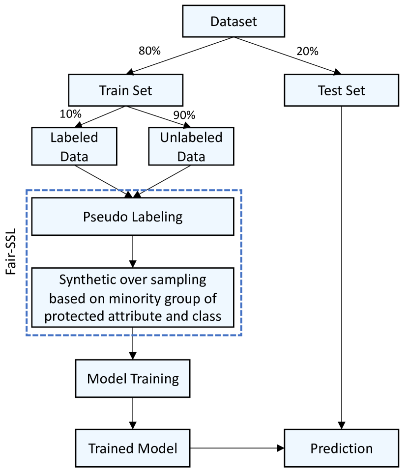
Figure 2. Framework of Fair-SSL

3.3. Synthetic Oversampling & Balancing

Our training data is now labeled. We can go for model training. But some prior works (Chen et al., 2018; Chakraborty et al., 2021) claimed that training data needs to be balanced in order to achieve fair prediction. Here data balancing means the number of examples based on protected attribute and class should be almost equal. We used the Fair-SMOTE technique (algorithm  1) by Chakraborty et al. (Chakraborty et al., 2021) to achieve that. Initial training data are divided into four groups (Favorable & Privileged, Favorable & Unprivileged, Unfavorable & Privileged, Unfavorable & Unprivileged). Initially, these subgroups are of unequal sizes. After synthetic oversampling, the training data becomes balanced based on target class and protected attribute i.e. above mentioned four groups become of equal sizes. We have now described all the major components of Fair-SSL that generates pseudo-labeled, and balanced training data from a very small set of labeled examples. Figure 2 shows Fair-SSL framework.

4. Results

We conducted our experiments on ten datasets (Table 1) and used three learners (logistic regression, random forest, support vector machine (svm)). Because of small size of datasets, prior fairness works (Chakraborty et al., 2020a; Kamishima et al., 2012; Calmon et al., 2017; Biswas and Rajan, 2020; Chakraborty et al., [n.d.], 2021) also chose simple models like us instead of deep learning models. We split the datasets using 5 fold cross-validation (train - 80%, test - 20%) and repeat 10 times with random seeds and finally report the median for every experiment. We compared Fair-SSL with three state-of-the-art fairness algorithms - Optimized Pre-processing (Calmon et al., 2017), Fairway (Chakraborty et al., 2020a), and Fair-SMOTE (Chakraborty et al., 2021) using Scott-Knott statistical test (Mittas and Angelis, 2013; Ghotra et al., 2015).

Table 3. RQ1, RQ2, and RQ4 results: “Default” means off-the-shelf logistic regression; Optimized Pre-processing(OP) (Calmon et al., 2017), Fairway (Chakraborty et al., 2020a), & Fair-SMOTE (Chakraborty et al., 2021) are state-of-the-art supervised methods. ST is self-training; LP is label-propagation; LS is label-spreading; CT is co-training. Darkest = 1st Rank;Lighter = 2nd Rank; Lightest = 3rd Rank; White = Last Rank (note: for the metrics with ‘+’ more is better and for the metrics with ‘-’ less is better). Rankings were calculated via Scott-Knott test.

Dataset	Protected Attribute	Algorithms	Recall (+)	False alarm (-)	Precision (+)	Accuracy (+)	F1 Score (+)	AOD (-)	EOD (-)	SPD (-)	DI (-)
		Default	0.46	0.07	0.69	0.83	0.54	0.12	0.24	0.21	0.56
		OP	0.42	0.09	0.61	0.76	0.51	0.04	0.03	0.04	0.14
		Fairway	0.25	0.04	0.71	0.72	0.42	0.02	0.03	0.04	0.11
		Fair-SMOTE	0.71	0.25	0.51	0.73	0.62	0.01	0.02	0.03	0.08
		Fair-SSL-ST	0.71	0.39	0.42	0.62	0.51	0.04	0.03	0.07	0.12
		Fair-SSL-LP	0.72	0.38	0.45	0.66	0.53	0.03	0.03	0.04	0.05
		Fair-SSL-LS	0.72	0.31	0.42	0.71	0.55	0.03	0.04	0.06	0.08
Adult Census Income	Sex	Fair-SSL-CT	0.76	0.35	0.44	0.68	0.57	0.06	0.04	0.03	0.08
		Default	0.67	0.38	0.66	0.64	0.61	0.09	0.19	0.18	0.28
		OP	0.71	0.36	0.64	0.62	0.60	0.04	0.03	0.05	0.08
		Fairway	0.56	0.22	0.57	0.58	0.58	0.03	0.03	0.06	0.08
		Fair-SMOTE	0.62	0.32	0.56	0.55	0.65	0.02	0.05	0.08	0.09
		Fair-SSL-ST	0.42	0.21	0.65	0.58	0.54	0.02	0.09	0.12	0.21
		Fair-SSL-LP	0.52	0.34	0.62	0.54	0.58	0.02	0.06	0.09	0.19
		Fair-SSL-LS	0.52	0.33	0.61	0.62	0.62	0.03	0.03	0.05	0.09
Compas	Sex	Fair-SSL-CT	0.49	0.28	0.62	0.61	0.57	0.03	0.02	0.05	0.07
		Default	0.25	0.07	0.70	0.78	0.34	0.05	0.08	0.06	0.35
		OP	0.28	0.06	0.65	0.70	0.32	0.01	0.02	0.03	0.09
		Fairway	0.21	0.04	0.67	0.67	0.33	0.01	0.04	0.03	0.12
		Fair-SMOTE	0.58	0.26	0.39	0.68	0.44	0.02	0.03	0.05	0.03
		Fair-SSL-ST	0.48	0.12	0.53	0.79	0.51	0.03	0.04	0.05	0.12
		Fair-SSL-LP	0.51	0.31	0.37	0.67	0.44	0.05	0.03	0.03	0.08
		Fair-SSL-LS	0.59	0.36	0.34	0.64	0.42	0.05	0.04	0.03	0.09
Default Credit	Sex	Fair-SSL-CT	0.59	0.35	0.36	0.65	0.44	0.03	0.03	0.05	0.08
		Default	0.73	0.21	0.76	0.77	0.77	0.08	0.22	0.24	0.31
		OP	0.72	0.20	0.74	0.75	0.75	0.04	0.05	0.02	0.04
		Fairway	0.71	0.17	0.73	0.71	0.71	0.04	0.03	0.05	0.06
		Fair-SMOTE	0.76	0.16	0.72	0.72	0.74	0.04	0.05	0.05	0.03
		Fair-SSL-ST	0.66	0.37	0.6	0.64	0.64	0.04	0.08	0.05	0.11
		Fair-SSL-LP	0.57	0.37	0.58	0.62	0.56	0.02	0.03	0.07	0.1
		Fair-SSL-LS	0.62	0.35	0.62	0.64	0.62	0.07	0.09	0.07	0.12
Bank Marketing	Age	Fair-SSL-CT	0.69	0.18	0.74	0.72	0.71	0.05	0.02	0.09	0.21
		Default	0.81	0.06	0.85	0.88	0.83	0.06	0.05	0.06	0.12
		OP	0.79	0.06	0.83	0.83	0.82	0.02	0.04	0.04	0.06
		Fairway	0.76	0.05	0.81	0.84	0.84	0.03	0.02	0.04	0.07
		Fair-SMOTE	0.87	0.10	0.84	0.87	0.86	0.04	0.04	0.04	0.08
		Fair-SSL-ST	0.84	0.14	0.83	0.83	0.83	0.03	0.02	0.01	0.03
		Fair-SSL-LP	0.83	0.19	0.82	0.82	0.83	0.04	0.03	0.07	0.21
		Fair-SSL-LS	0.84	0.14	0.79	0.84	0.82	0.03	0.02	0.05	0.05
Student Performance	Sex	Fair-SSL-CT	0.84	0.09	0.84	0.85	0.83	0.04	0.02	0.03	0.08

Table 4. RQ2 results: Comparing Fair-SSL with three prior works based on results of 10 datasets and three learners. Number of wins, ties, and losses are calculated using Scott-Knott ranks. Pink cells show Fair-SSL is performing similar/better than others.

		Recall	False alarm	Precision	Accuracy	F1 Score	AOD	EOD	SPD	DI	Total
	Optimized Pre-processing vs Fair-SSL
1	Win	8	2	4	3	10	2	2	1	2	34
2	Tie	21	25	27	28	24	32	33	32	32	254
3	Loss	7	9	5	5	2	2	1	3	2	36
4	Win + Tie	29	27	31	31	34	34	35	33	34	288/324
	Fairway vs Fair-SSL
5	Win	10	2	5	5	19	2	3	3	4	53
6	Tie	24	17	24	27	14	30	31	32	31	230
7	Loss	2	17	7	4	3	4	2	1	1	41
8	Win + Tie	34	19	29	33	33	32	34	35	35	283/324
	Fair-SMOTE vs Fair-SSL
9	Win	1	3	2	3	3	1	2	2	2	19
10	Tie	28	30	30	28	29	34	33	32	31	275
11	Loss	7	3	4	5	4	1	1	2	3	30
12	Win + Tie	29	33	32	31	32	35	35	34	33	294/324

Table 5. RQ3 results: The change of accuracy, F1, AOD and EOD for Fair-SSL with increasing size of labeled training data.Dark = 1st Rank;Light = 2nd Rank; White = Last Rank

Dataset Protected Attribute Size of Labeled Set Accuracy (+) F1 Score (+) AOD (-) EOD (-) 1% 0.61 0.44 0.04 0.06 5% 0.68 0.51 0.03 0.02 10% 0.71 0.54 0.03 0.03 Adult Sex 20% 0.71 0.58 0.02 0.02 1% 0.47 0.44 0.07 0.12 5% 0.57 0.54 0.06 0.06 10% 0.58 0.61 0.03 0.07 Compas Sex 20% 0.61 0.64 0.01 0.05 1% 0.67 0.65 0.18 0.12 5% 0.78 0.75 0.05 0.07 10% 0.83 0.82 0.02 0.02 Student Sex 20% 0.85 0.83 0.02 0.01

Table 3 answers the question. It contains the results for five datasets. “Default” rows signify when a logistic regression model is trained on the available labeled training data with no modification. We see for every dataset, the values of AOD, EOD, SPD, and DI are very high indicating bias in prediction. For every dataset, the last four rows show the results of Fair-SSL with four different algorithms used as pseudo-labeler inside. That means, 10% labeled training data is used and rest of the training data has been pseudo-labeled. After that combined training data is oversampled to be balanced based on protected attribute and class. Finally, the generated data has been used for model training. We see all four versions of Fair-SSL significantly reduce the values of four bias metrics (AOD, EOD, SPD, and DI) for all the datasets. The answer for RQ1 is “Yes, Fair-SSL can significantly reduce bias. It improves recall and F1 and sometimes damages false alarm, and accuracy. Prior fairness works (Chakraborty et al., 2020a; Kamiran et al., 2018; Kamiran and Calders, 2012; Zhang et al., 2018; Calmon et al., 2017) also damaged performance of the model while achieving fairness. This is called the “fairness-performance” trade-off in the literature.”

Here we are comparing Fair-SSL with three other state-of-the-art bias mitigation algorithms - Optimized Pre-processing (Calmon et al., 2017), Fairway (Chakraborty et al., 2020a) and Fair-SMOTE (Chakraborty et al., 2020a). If we look at Table 3, the last four columns are bias scores where Fair-SSL is performing as good as the others. In case of performance metrics (first five columns), we see it is losing sometimes but not by much. To get a clear picture, we take a look at Table 4. Here we show the summarized results for all ten datasets (Adult and Compas have two protected attributes each, i.e. 10 + 2 = 12 cases) and three learners (logistic regression, random forest, and svm). We have implemented four different versions of Fair-SSL (ST, LP, LS, CT). For comparison purpose, for every dataset, we have created a validation set (20%) from the train set. On the validation set, we tried all four versions of Fair-SSL and chose the best one to run on the test set. Thus, Table 4 contains comparison of the best version of Fair-SSL (best is selected based on validation results) with three other bias mitigation algorithms. We see in bias scores, Fair-SSL is as good as other three. In ‘recall’ and ‘F1 score’, it performs better than Optimized Pre-processing and Fairway. One important point to mention here is that other three algorithms take advantage of full training data where Fair-SSL takes only 10% of labeled training data. The answer for RQ2 is “Fair-SSL is as good as others in reducing bias, sometimes better in “recall” and “F1” than Optimized Pre-processing and Fairway.”

Semi-supervised algorithms work with a small amount of labeled data and a large amount of unlabeled data. However, it is crucial to know how much labeled data is needed to start. Table 5 shows results for three datasets where size of the initial fairly labeled set has been varied from 1% to 20%. Here also we used the best version of Fair-SSL based on validation set results. We see the trend of increasing accuracy, F1, and decreasing AOD, EOD with increasing size of initial fairly labeled set. Even when using 5% labeled training data, we see Fair-SSL can significantly reduce bias. However, for accuracy and F1, Fair-SSL with 10% labeled training data performs much better than 5% version and very similar to 20% version. Hence, to answer RQ3, we say that “Fair-SSL can significantly reduce bias even when a very small amount of labeled data points are available. Performance of Fair-SSL gets better with increasing size of initial labeled training set.”

The results so far can be summarized as follows: semi-supervised algorithms can be useful to augment bias mitigation process. That raises our next research question: which one of our four different semi-supervised techniques performs the best in this context?

Table 3 shows all four versions of Fair-SSL are reducing the bias scores. In case of performance metrics (the first five columns), all four of them are doing just the same (with minor differences). That means there is no way to choose one best method among the four methods. This reminds us of the popular “No free lunch theorem” for machine learning (Fedden, 2017). We can certainly say semi-supervised pseudo-labeling improves fairness but which one is the best depends on the specific dataset.

We also compared the execution time of all four semi-supervised algorithms. We found out label propagation is the slowest and self-training is the fastest method. Hence, our answer for RQ4 is “Semi-supervised techniques help but there is no winner based on performance. We should try all the approaches for a particular dataset to find out the best one. However, based on execution time, self-training works the fastest.”

5. Discussion & Limitation

What does make Fair-SSL unique and more useful than prior works?
Inexpensive - Real world data comes as a mixture of labeled and unlabeled form. Hiring Crowdsource workers for labeling can be very expensive (Tu et al., 2020b). Fair-SSL pseudo-labeler is a cheap alternative.
Performance - Fair-SSL can significantly reduce bias, improves recall & F1 score and sometimes damages accuracy, false alarm. All the prior supervised works (except Fair-SMOTE (Chakraborty et al., 2021)) damage performance to achieve fairness (Biswas and Rajan, 2020; Kleinberg et al., 2016; Tolan et al., 2019). Performance wise Fair-SSL is similar to Fair-SMOTE but cheaper (uses 10% data labels).
Model-agnostic - Fair-SSL is a data pre-processor. That means after pseudo-labeling the data, any supervised model can be used for final prediction. Thus Fair-SSL is model agnostic.

Fair-SSL does come with some limitations. We have used ten well-known datasets, three classification models, and four fairness metrics. Most of the prior works (Calmon et al., 2017; Galhotra et al., 2017; Zhang et al., 2018; Kamiran et al., 2018; Chakraborty et al., [n.d.]) used one or two datasets and metrics. In future, we will explore more datasets and more learners. One assumption of evaluating our experiments is the test data is unbiased. Prior fairness studies also made similar assumption (Chakraborty et al., 2021; Biswas and Rajan, 2020; Chakraborty et al., [n.d.]). SSL can be helpful when bias comes from improper data labels or sampling. But it can not solve some other bias causing factors such as objective function bias, homogenization bias (Das and Donini, 2020), and feature correlation bias (Zhang et al., 2016a).

6. Conclusion

Fairness in machine learning software has become a serious concern in the software engineering community. Prior fairness works mainly used supervised approaches that require data with ground truth labels. However, good quality labeled data is not always available in real-life. Keeping that in concern, this paper shows how semi-supervised techniques can be used to achieve fairness by using only 10% labeled training data. We believe our work will encourage future software researchers to work in the software fairness domain.

References

- (1)
- ADU (1994) 1994. UCI:Adult Data Set. (1994). http://mlr.cs.umass.edu/ml/datasets/Adult
- GER (2000) 2000. UCI:Statlog (German Credit Data) Data Set. (2000). https://archive.ics.uci.edu/ml/datasets/Statlog+(German+Credit+Data)
- HEA (2001) 2001. UCI:Heart Disease Data Set. (2001). https://archive.ics.uci.edu/ml/datasets/Heart+Disease
- USA (2007) 2007. Situation Testing for Employment Discrimination in the United States of America. https://www.cairn.info/revue-horizons-strategiques-2007-3-page-17.htm
- for (2011) 2011. The Algorithm That Beats Your Bank Manager. (2011). https://www.forbes.com/sites/parmyolson/2011/03/15/the-algorithm-that-beats-your-bank-manager/#15da2651ae99
- STU (2014) 2014. Student Performance Data Set. (2014). https://archive.ics.uci.edu/ml/datasets/Student+Performance
- MEP (2015) 2015. Medical Expenditure Panel Survey. (2015). https://meps.ahrq.gov/mepsweb/data_stats/download_data_files_detail.jsp?cboPufNumber=HC-181
- COM (2015) 2015. propublica/compas-analysis. (2015). https://github.com/propublica/compas-analysis
- MEP (2016) 2016. Medical Expenditure Panel Survey. (2016). https://meps.ahrq.gov/mepsweb/data_stats/download_data_files_detail.jsp?cboPufNumber=HC-192
- DEF (2016) 2016. UCI:Default of credit card clients Data Set. (2016). https://archive.ics.uci.edu/ml/datasets/default+of+credit+card+clients
- BAN (2017) 2017. Bank Marketing UCI. (2017). https://www.kaggle.com/c/bank-marketing-uci
- HOM (2017) 2017. THome Credit Default Risk. (2017). https://www.kaggle.com/c/home-credit-default-risk
- AIF (2018) 2018. AI Fairness 360: An Extensible Toolkit for Detecting, Understanding, and Mitigating Unwanted Algorithmic Bias. (10 2018). https://github.com/IBM/AIF360
- Ama (2018) 2018. Amazon scraps secret AI recruiting tool that showed bias against women. (Oct 2018). https://www.reuters.com/article/us-amazon-com-jobs-automation-insight/amazon-scraps-secret-ai-recruiting-tool-that-showed-bias-against-women-idUSKCN1MK08G
- EU (2018) 2018. Ethics Guidelines for Trustworthy Artificial Intelligence. https://ec.europa.eu/digital-single-market/en/news/ethics-guidelines-trustworthy-ai
- FAI (2018) 2018. FAIRWARE 2018:International Workshop on Software Fairness. (2018). http://fairware.cs.umass.edu/
- Med (2018) 2018. Health care start-up says A.I. can diagnose patients better than humans can, doctors call that ‘dubious’. CNBC (June 2018). https://www.cnbc.com/2018/06/28/babylon-claims-its-ai-can-diagnose-patients-better-than-doctors.html
- Ski (2018) 2018. Study finds gender and skin-type bias in commercial artificial-intelligence systems. (2018). http://news.mit.edu/2018/study-finds-gender-skin-type-bias-artificial-intelligence-systems-0212
- EXP (2019) 2019. EXPLAIN 2019. (2019). https://2019.ase-conferences.org/home/explain-2019
- hir (2020) 2020. HireVue Assessment Tools. https://www.hirevue.com/
- skl (2021a) 2021a. Effect of varying threshold for self-training. (2021). https://scikit-learn.org/stable/auto_examples/semi_supervised/plot_self_training_varying_threshold.html#sphx-glr-auto-examples-semi-supervised-plot-self-training-varying-threshold-py
- Fai (2021) 2021. Fairlearn. https://fairlearn.org/
- goo (2021) 2021. Google Cloud Pricing. https://cloud.google.com/ai-platform/data-labeling/pricing
- log (2021) 2021. Log-linear Models and Conditional Random Fields. (2021). http://videolectures.net/cikm08_elkan_llmacrf/
- 3ds (2021) 2021. The most costly thing in Machine Learning Algorithms is labeling. https://3dsignals.com/blog/the-most-costly-thing-in-machine-learning-algorithms-is-labeling/
- skl (2021b) 2021b. Probability calibration. (2021). https://scikit-learn.org/stable/modules/calibration.html#calibration
- Aggarwal et al. (2019) Aniya Aggarwal, Pranay Lohia, Seema Nagar, Kuntal Dey, and Diptikalyan Saha. 2019. Black Box Fairness Testing of Machine Learning Models (ESEC/FSE 2019). ACM, New York, NY, USA, 625–635. https://doi.org/10.1145/3338906.3338937
- Angell et al. ([n.d.]) Rico Angell, Brittany Johnson, Yuriy Brun, and Alexandra Meliou. [n.d.]. Themis: Automatically Testing Software for Discrimination (ESEC/FSE 18). 5. https://doi.org/10.1145/3236024.3264590
- Berk et al. (2017) Richard Berk, Hoda Heidari, Shahin Jabbari, Michael Kearns, and Aaron Roth. 2017. Fairness in Criminal Justice Risk Assessments: The State of the Art. arXiv:stat.ML/1703.09207
- Biswas and Rajan (2020) Sumon Biswas and Hridesh Rajan. 2020. Do the machine learning models on a crowd sourced platform exhibit bias? an empirical study on model fairness. Proceedings of the 28th ACM Joint Meeting on European Software Engineering Conference and Symposium on the Foundations of Software Engineering (Nov 2020). https://doi.org/10.1145/3368089.3409704
- Blum and Mitchell (1998) Avrim Blum and Tom Mitchell. 1998. Combining Labeled and Unlabeled Data with Co-Training (COLT’ 98). Association for Computing Machinery, New York, NY, USA, 92–100. https://doi.org/10.1145/279943.279962
- Brun and Meliou (2018) Yuriy Brun and Alexandra Meliou. 2018. Software Fairness (ESEC/FSE 2018). Association for Computing Machinery, New York, NY, USA, 754–759. https://doi.org/10.1145/3236024.3264838
- Caliskan et al. (2017) Aylin Caliskan, Joanna J. Bryson, and Arvind Narayanan. 2017. Semantics derived automatically from language corpora contain human-like biases. Science 356, 6334 (2017), 183–186. https://doi.org/10.1126/science.aal4230 arXiv:https://science.sciencemag.org/content/356/6334/183.full.pdf
- Calmon et al. (2017) Flavio Calmon, Dennis Wei, Bhanukiran Vinzamuri, Karthikeyan Natesan Ramamurthy, and Kush R Varshney. 2017. Optimized Pre-Processing for Discrimination Prevention. In Advances in Neural Information Processing Systems 30, I. Guyon, U. V. Luxburg, S. Bengio, H. Wallach, R. Fergus, S. Vishwanathan, and R. Garnett (Eds.). Curran Associates, Inc., 3992–4001. http://papers.nips.cc/paper/6988-optimized-pre-processing-for-discrimination-prevention.pdf
- Chakraborty et al. (2021) Joymallya Chakraborty, Suvodeep Majumder, and Tim Menzies. 2021. Bias in Machine Learning Software: Why? How? What to Do? (ESEC/FSE 2021). Association for Computing Machinery, New York, NY, USA, 429–440. https://doi.org/10.1145/3468264.3468537
- Chakraborty et al. (2020a) Joymallya Chakraborty, Suvodeep Majumder, Zhe Yu, and Tim Menzies. 2020a. Fairway: A Way to Build Fair ML Software (ESEC/FSE 2020). Association for Computing Machinery, New York, NY, USA, 654–665. https://doi.org/10.1145/3368089.3409697
- Chakraborty et al. (2020b) Joymallya Chakraborty, Kewen Peng, and Tim Menzies. 2020b. Making Fair ML Software Using Trustworthy Explanation (ASE ’20). Association for Computing Machinery, New York, NY, USA, 1229–1233. https://doi.org/10.1145/3324884.3418932
- Chakraborty et al. ([n.d.]) Joymallya Chakraborty, Tianpei Xia, Fahmid M. Fahid, and Tim Menzies. [n.d.]. Software Engineering for Fairness: A Case Study with Hyperparameter Optimization. ACM/IEEE International Conference on Automated Software Engineering - ASE 2019 ([n. d.]). https://2019.ase-conferences.org/track/ase-2019-Late-Breaking-Results?track=ASE%20Late%20Breaking%20Results
- Chen et al. (2018) Irene Chen, Fredrik D. Johansson, and David Sontag. 2018. Why Is My Classifier Discriminatory? arXiv:stat.ML/1805.12002
- Das and Donini (2020) Sanjiv Das and Michele Donini. 2020. Fairness Measures for Machine Learning in Finance. arXiv:https://pages.awscloud.com/rs/112-TZM-766/images/Fairness.Measures.for.Machine.Learning.in.Finance.pdf
- Fedden (2017) Leon Fedden. 2017. The No Free Lunch Theorem (or why you can’t have your cake and eat it). https://medium.com/@LeonFedden/the-no-free-lunch-theorem-62ae2c3ed10c
- Galhotra et al. (2017) Sainyam Galhotra, Yuriy Brun, and Alexandra Meliou. 2017. Fairness testing: testing software for discrimination. Proceedings of the 2017 11th Joint Meeting on Foundations of Software Engineering - ESEC/FSE 2017 (2017). https://doi.org/10.1145/3106237.3106277
- Ghotra et al. (2015) Baljinder Ghotra, Shane McIntosh, and Ahmed E Hassan. 2015. Revisiting the impact of classification techniques on the performance of defect prediction models. In 37th ICSE-Volume 1. IEEE Press, 789–800.
- Hardt et al. (2016) Moritz Hardt, Eric Price, and Nathan Srebro. 2016. Equality of Opportunity in Supervised Learning. arXiv:cs.LG/1610.02413
- Hyun et al. (2020) Minsung Hyun, Jisoo Jeong, and Nojun Kwak. 2020. Class-Imbalanced Semi-Supervised Learning. arXiv:cs.LG/2002.06815
- James Manyika and Presten (2019) Jake Silberg James Manyika and Brittany Presten. 2019. What Do We Do About the Biases in AI? https://hbr.org/2019/10/what-do-we-do-about-the-biases-in-ai
- Jiang and Nachum (2019) Heinrich Jiang and Ofir Nachum. 2019. Identifying and Correcting Label Bias in Machine Learning. arXiv:cs.LG/1901.04966
- Kamiran and Calders (2012) Faisal Kamiran and Toon Calders. 2012. Data preprocessing techniques for classification without discrimination. Knowledge and Information Systems 33, 1 (01 Oct 2012), 1–33. https://doi.org/10.1007/s10115-011-0463-8
- Kamiran et al. (2018) Faisal Kamiran, Sameen Mansha, Asim Karim, and Xiangliang Zhang. 2018. Exploiting Reject Option in Classification for Social Discrimination Control. Inf. Sci. (2018). https://doi.org/10.1016/j.ins.2017.09.064
- Kamishima et al. (2012) Toshihiro Kamishima, Shotaro Akaho, Hideki Asoh, and Jun Sakuma. 2012. Fairness-Aware Classifier with Prejudice Remover Regularizer. In Machine Learning and Knowledge Discovery in Databases, Peter A. Flach, Tijl De Bie, and Nello Cristianini (Eds.). Springer Berlin Heidelberg, Berlin, Heidelberg, 35–50.
- Kleinberg et al. (2016) Jon Kleinberg, Sendhil Mullainathan, and Manish Raghavan. 2016. Inherent Trade-Offs in the Fair Determination of Risk Scores. arXiv:cs.LG/1609.05807
- Li et al. (2011) Shoushan Li, Zhongqing Wang, Guodong Zhou, and Sophia Yat Mei Lee. 2011. Semi-Supervised Learning for Imbalanced Sentiment Classification (IJCAI’11). AAAI Press, 1826–1831.
- Mittas and Angelis (2013) Nikolaos Mittas and Lefteris Angelis. 2013. Ranking and clustering software cost estimation models through a multiple comparisons algorithm. IEEE Transactions on software engineering 39, 4 (2013), 537–551.
- Shahriari and Shahriari (2017) Kyarash Shahriari and Mana Shahriari. 2017. IEEE standard review — Ethically aligned design: A vision for prioritizing human wellbeing with artificial intelligence and autonomous systems. In 2017 IEEE Canada International Humanitarian Technology Conference (IHTC). 197–201. https://doi.org/10.1109/IHTC.2017.8058187
- Simons (2020) Ted Simons. 2020. Addressing issues of fairness and bias in AI. https://blogs.thomsonreuters.com/answerson/ai-fairness-bias/
- Tatman (2017) Rachael Tatman. 2017. Gender and Dialect Bias in YouTube’s Automatic Captions. In Proceedings of the First ACL Workshop on Ethics in Natural Language Processing. Association for Computational Linguistics, Valencia, Spain, 53–59. https://doi.org/10.18653/v1/W17-1606
- Tolan et al. (2019) Songül Tolan, Marius Miron, Emilia Gómez, and Carlos Castillo. 2019. Why Machine Learning May Lead to Unfairness: Evidence from Risk Assessment for Juvenile Justice in Catalonia (ICAIL ’19). Association for Computing Machinery, New York, NY, USA, 83–92. https://doi.org/10.1145/3322640.3326705
- Tu and Menzies (2021) Huy Tu and Tim Menzies. 2021. FRUGAL: Unlocking SSL for Software Analytics. arXiv: Machine Learning (2021).
- Tu et al. (2020a) Huy Tu, Zhe Yu, and Tim Menzies. 2020a. Better Data Labelling with EMBLEM (and how that Impacts Defect Prediction). arXiv:cs.SE/1905.01719
- Tu et al. (2020b) Huy Tu, Zhe Yu, and Tim Menzies. 2020b. Better Data Labelling with EMBLEM (and how that Impacts Defect Prediction). IEEE Transactions on Software Engineering (2020), 1–1. https://doi.org/10.1109/TSE.2020.2986415
- Udeshi et al. (2018) Sakshi Udeshi, Pryanshu Arora, and Sudipta Chattopadhyay. 2018. Automated directed fairness testing. Proceedings of the 33rd ACM/IEEE International Conference on Automated Software Engineering - ASE 2018 (2018). https://doi.org/10.1145/3238147.3238165
- Wu (2016) Dapeng Oliver Wu. 2016. Network Science and Applications. Technical Report.
- Xiang (2019) Mark Xiang. 2019. Human Bias in Machine Learning. https://towardsdatascience.com/bias-what-it-means-in-the-big-data-world-6e64893e92a1
- Yan et al. (2020) Shen Yan, Hsien-te Kao, and Emilio Ferrara. 2020. Fair Class Balancing: Enhancing Model Fairness without Observing Sensitive Attributes (CIKM ’20). Association for Computing Machinery, New York, NY, USA, 1715–1724. https://doi.org/10.1145/3340531.3411980
- Yarowsky (1995) David Yarowsky. 1995. Unsupervised Word Sense Disambiguation Rivaling Supervised Methods (ACL ’95). Association for Computational Linguistics, USA, 189–196. https://doi.org/10.3115/981658.981684
- Yu et al. (2019) Zhe Yu, Fahmid Fahid, Tim Menzies, Gregg Rothermel, Kyle Patrick, and Snehit Cherian. 2019. TERMINATOR: Better Automated UI Test Case Prioritization (ESEC/FSE 2019). Association for Computing Machinery, New York, NY, USA, 883–894. https://doi.org/10.1145/3338906.3340448
- Yu et al. (2019) Z. Yu, C. Theisen, L. Williams, and T. Menzies. 2019. Improving Vulnerability Inspection Efficiency Using Active Learning. IEEE Transactions on Software Engineering (2019), 1–1. https://doi.org/10.1109/TSE.2019.2949275
- Zhang et al. (2018) Brian Hu Zhang, Blake Lemoine, and Margaret Mitchell. 2018. Mitigating Unwanted Biases with Adversarial Learning. arXiv:cs.LG/1801.07593
- Zhang et al. (2016a) Lu Zhang, Yongkai Wu, and Xintao Wu. 2016a. A causal framework for discovering and removing direct and indirect discrimination. arXiv:cs.LG/1611.07509
- Zhang et al. (2016b) Lu Zhang, Yongkai Wu, and Xintao Wu. 2016b. Situation Testing-Based Discrimination Discovery: A Causal Inference Approach (IJCAI’16). AAAI Press, 2718–2724.
- Zhang et al. (2020a) Peixin Zhang, Jingyi Wang, Jun Sun, Xingen Dong, Jin Song Dong, and Ting Dai. 2020a. White-Box Fairness Testing through Adversarial Sampling (ICSE ’20). Association for Computing Machinery, New York, NY, USA, 949–960. https://doi.org/10.1145/3377811.3380331
- Zhang et al. (2020b) Tao Zhang, tianqing zhu, Jing Li, Mengde Han, Wanlei Zhou, and Philip Yu. 2020b. Fairness in Semi-supervised Learning: Unlabeled Data Help to Reduce Discrimination. IEEE Transactions on Knowledge and Data Engineering (2020), 1–1. https://doi.org/10.1109/tkde.2020.3002567
- Zhang et al. (2017) Zhi-Wu Zhang, Xiao-Yuan Jing, and Tie-Jian Wang. 2017. Label Propagation Based Semi-Supervised Learning for Software Defect Prediction. Automated Software Engg. 24, 1 (March 2017), 47–69. https://doi.org/10.1007/s10515-016-0194-x
- Zhou et al. (2004) Dengyong Zhou, Olivier Bousquet, Thomas Lal, Jason Weston, and Bernhard Schölkopf. 2004. Learning with Local and Global Consistency. In Advances in Neural Information Processing Systems, S. Thrun, L. Saul, and B. Schölkopf (Eds.), Vol. 16. MIT Press. https://proceedings.neurips.cc/paper/2003/file/87682805257e619d49b8e0dfdc14affa-Paper.pdf
- Zhu (2006) Xiaojin Zhu. 2006. Semi-Supervised Learning Literature Survey. http://pages.cs.wisc.edu/~jerryzhu/pub/ssl_survey.pdf
- Zhu and Ghahramani (2002) Xiaojin Zhu and Zoubin Ghahramani. 2002. Learning from Labeled and Unlabeled Data with Label Propagation. Technical Report.