The galaxy power spectrum on the lightcone: deep, wide-angle redshift surveys and the turnover scale

Abstract

We derive expressions for the survey-window convolved galaxy power spectrum in real space for a full sky and deep redshift survey, but taking into account the geometrical lightcone effect. We investigate the impact of using the standard mean redshift approximation as a function of survey depth, and show that this assumption can lead to both an overall amplitude suppression and scale-dependent error when compared to the ‘true’ spectrum. However, we also show that by using a carefully chosen ‘effective fixed-time’, one can find a range of scales where the approximation to the full model is highly accurate, but only on a more restricted set of scales. We validate the theory by constructing dark matter and galaxy lightcone mock surveys from a large $N$-body simulation with a high cadence of snapshots. We do this by solving the light cone equation exactly for every particle, where the particle worldlines are obtained in a piecewise fashion with cubic interpolation between neighbouring snapshots. We find excellent agreement between our measurements and the theory ($\sim\pm 5\%$) over scales $(0.004\,h\,{\rm Mpc}^{-1}\leq k\leq 0.54\,h\,{\rm Mpc}^{-1})$ and for a variety of magnitude limits. Finally, we look to see how accurately we can measure the turnover scale of the galaxy power spectrum $k_{0}$. Using the lightcone mocks we show that one can detect the turnover scale with a probability $P\geq 95\%$ in an all-sky catalogue limited to an apparent magnitude $m_{\rm lim}\sim 21$. We also show that the detection significance would remain high for surveys with $m_{\rm lim}\sim 22$ and $20\%$ sky coverage.

1 Introduction

The next decade will herald significant advances in the quantity of high fidelity data for mapping the large-scale distribution of galaxies. This will be facilitated through a series of exciting new wide-field observatories, such as the spectroscopic missions DESI [1], 4MOST [2], the ESA Euclid space mission [3] and the NASA mission SPHEREx [4]. These will be complemented by the panchromatic imaging surveys like LSST [5] and Euclid. Together these observatories will map the galaxy distribution out to high redshift and over significant fractions of the full-sky, and will thus chart effective volumes that approach the observable size of our Universe out to a given redshift [4]. All of these surveys will be able to make unprecedented measurements of the statistical properties of the spatial distribution of galaxies.

The lowest order spatial statistic of interest is the correlation function, or equivalently its Fourier-space dual the power spectrum. The full shape and amplitude of the matter power spectrum carries a great deal of information about the cosmological model and the primordial distribution of the initial density fluctuations [6]. However, the extraction of this information is complicated by a number of effects: first, the initial linear density perturbations become nonlinearly coupled due to gravitational instability [7, 8]. Understanding this process is further complicated by the fact that the matter distribution is built from the weighted densities of baryons, cold dark matter and massive neutrinos, each component of which needs to be propagated into the nonlinear regime through careful modelling [see for example 9, 10, 11]. Second, galaxies are a biased set of tracers for the matter distribution, and may in full generality be a nonlinear, time-dependent, non-local, stochastic sampling of the matter, and this connection varies with the types of galaxies that are selected [12, 13, 14, 15, 16, 17, 18]. Third, owing to the fact that galaxy positions are inferred from their measured redshifts there is a distortion in the mapping from observed to true position, which arises due to the fact that galaxies have peculiar velocities relative to the Hubble flow – redshift space distortions [19, 20, 21].

To this one can also add the lightcone effect, which has surfaced in this recent era of precision cosmology – for deep surveys one has to account for the fact that we are correlating galaxy positions on the observer’s past lightcone [22, 23]. Furthermore, there are additional corrections that arise due to general relativistic effects and also the magnification effects that all arise due to light propagation in a weakly perturbed spacetime [24, 25]. Another source of error arises from the assumption of a wrong cosmological model, in principle this could be overcome by simply recalculating the statistic of interest for every assumed cosmological model to be tested [26, 27]. Together, these effects can all be thought of as modelling problems and one should look to account for them when comparing to measurements. Besides these ‘physical’ effects one can add a number of important ‘observational’ effects that also need to be carefully taken into account: the survey mask; star–galaxy classification; curved sky effects; fibre collision and completeness; accurate flux calibration across the survey; K-corrections, etc.

In this paper we focus on a subset of these issues. Our goal here is to build up the methodology for forward modelling the theory of the real space, 3D galaxy power spectrum in a survey which spans a significant fraction of the sky and thus requires us to take into account wide-angle clustering effects and one that is also deep and so requires us to handle the lightcone effect. This means that we will need to take into account: the convolution with the survey window function, the lightcone effect, including the unequal time correlators and work on the curved sky. We reserve exploration of redshift-space distortions and the power-spectrum multipoles for future work. Our aim here is thus to evolve the estimation and forward modelling analysis methodology to the next level [28, 29, 30, 31, 32].

Regarding the lightcone effect, our work here is most closely inspired by that of [22] and we provide alternate derivations of results from that work that are easier to evaluate, but our results go beyond that work in a number of key ways. First, working with the spherical-Fourier-Bessel (hereafter sFB) expansion of the theory, we find expressions that are simpler to compute. Second, we include galaxy weighting and luminosity dependent galaxy bias. Third, we derive the shot-noise and show that its form remains as that found by [33]. Fourth, we include general expressions with a survey mask. We validate all of this with a series of deep full-sky galaxy mocks derived from $N$-body simulations.

In this work we will make use of the sFB harmonic analysis of a galaxy redshift survey and this approach has a long history in cosmology [34, 35, 36, 37, 38, 39, 40, 41, 42, 43], and we will take many of our cues from these important works. Furthermore, as discussed in [44], for a more exhaustive analysis of galaxy clustering for wide-angled surveys two schools of thought have emerged in recent years: one is to develop the power spectrum multipoles, following the estimator style of [45, 46]; the other is to work in the sFB framework from the start. The former approach has the problem of requiring complex estimators, but is easier to model. The latter allows us to make use of the decomposition of the problem into radial and angular modes, but has been highlighted as harder to model. For our work, since we are restricting our attention to the monopole of the power spectrum, there is no great complexity in how we estimate it [46] from data. That is not to say that there are no subtleties in its estimation. Our effort therefore mainly goes into modelling this signal for a wide-angle survey, that is also deep.

An additional important science driver for future surveys is the question of: How well can we detect the ‘turnover scale’ of the matter power spectrum. This length scale denotes the point of maximum amplitude of the matter power spectrum and for the $\Lambda$CDM model is a direct imprint of the epoch of matter-radiation equality in the early stages of the Universe. A number of previous works have examined this issue [47, 48, 49]. However, here we now relax some of the simplifying assumptions and use our improved formalism to attempt to address questions on this topic.

The paper breaks down as follows: In §2 and §3 we develop the theory of the galaxy power spectrum on the curved-sky, past lightcone. In §4 we explore some approximate forms to our model that can make it more numerically tractable. Then in §5 we describe how we create mock lightcone catalogues, detail the process used to estimate the power spectrum from these mocks, and then make comparisons to theory in §6. We then explore the ability to constrain the power spectrum turnover scale from our measured spectra in §7. Finally, in §8 we summarise our findings, conclude and discuss future work.

2 Theoretical background

We now review some of the key aspects of the background theory necessary for what follows. Note that we will neglect the effects of time delay and photon deviations that are required to describe a full general relativistic treatment of light propagation on the perturbed past lightcone.

2.1 The past lightcone

To begin, we assume that the unperturbed background spacetime is a spatially flat, homogeneous and isotropic, spacetime. Hence, in spherical coordinates the differential FLRW line element can be written as:

$$ds^{2}=a(\eta)^{2}\left[c^{2}d\eta^{2}-d\chi^{2}-\chi^{2}d\theta^{2}-\chi^{2}\sin^{2}\theta d\phi^{2}\right]\ ,$$ (2.1)

where $\eta$ is the conformal time, $a(\eta)$ is the scale factor, $\chi$ is the comoving radial geodesic distance, $c$ is the speed of light and $\theta$ and $\phi$ are the usual polar angles, which we denote collectively as $\bm{\gamma}\rightarrow(\theta,\phi)$. A light signal emitted at spacetime point $(\eta_{1},\chi_{1},\bm{\gamma}_{1})$ will be received by an observer located at the origin of our coordinate system at spacetime point $(\eta_{2},0,{\bf 0})$. From the FLRW line element, we see that points on the past lightcone are required to obey the following relation between the radial comoving distance from the observer and the redshift:

$$r(z)=\left|\int^{0}_{r}d\chi\right|=\int_{\eta_{1}}^{\eta_{2}}cd\eta=\int_{0}^{z}\frac{cdz^{\prime}}{H(z^{\prime})}\ ,$$ (2.2)

where the redshift is related to the expansion factor as $z=1/a(\eta)-1$ and the Hubble rate is $H(z)\equiv a^{-2}(da/d\eta)$. This can be calculated from the Friedmann equations, and for the case of flat $\Lambda$CDM is given by:

$$H^{2}(z)=H_{0}^{2}\left[\Omega_{\rm m,0}(1+z)^{3}+\Omega_{\Lambda,0}\right]\ ,$$ (2.3)

where $\Omega_{\rm m,0}$ and $\Omega_{\Lambda,0}$ are the present day matter and cosmological constant density parameters, respectively. Since we are assuming a flat model here, we also have $\Omega_{\rm m,0}+\Omega_{\Lambda,0}=1$.

2.2 The galaxy overdensity field on the past lightcone

Following [22], let us define the galaxy density field at time $\eta$, with radial and angular positions $(\chi,\bm{\gamma})$, as:

$$n(\eta,\chi,\bm{\gamma})=n_{0}(\eta)\left[1+\Delta(\eta,\chi,\bm{\gamma})\right]\ ,$$ (2.4)

where $n_{0}(\eta)$ is the mean number density of galaxies at time $\eta$ and $\Delta(\eta,\chi,\bm{\gamma})$ is the density contrast of galaxies at the position. Thus on the past lightcone the number density is written:

$$n^{\rm LC}({\bf r})=\left.n_{0}(\eta)\left[1+\Delta(\eta,\chi,\bm{\gamma})\right]\frac{}{}\right|_{\eta\rightarrow\eta_{0}-r/c,\chi\rightarrow r}\ ,$$ (2.5)

where ${\bf r}\rightarrow(r,\bm{\gamma})$ and where $\eta_{0}$ is the present day conformal time. We can also define another useful quantity, which gives the background density on the lightcone:

$$n^{\rm LC}_{0}(\eta)=\left.n_{0}(\eta)\frac{}{}\right|_{\eta\rightarrow\eta_{0}-r/c}\ .$$ (2.6)

Let us next define the overdensity contrast of galaxies on the past lightcone as:

$$\Delta\!^{\rm LC}({\bf r})\equiv\frac{n^{\rm LC}({\bf r})-n_{0}^{\rm LC}(r)}{n_{0}^{\rm LC}(r)}=\Delta(\eta^{\prime},{\bf r})\ .$$ (2.7)

where we have defined $\eta^{\prime}\equiv\eta_{0}-r/c$, which gives the conformal time at which the density field is recorded on the past lightcone. Note that the second equality is important and means that the density contrast on the lightcone can be rewritten in terms of the density field at time $\eta^{\prime}$. In what follows we will make extensive use of this property.

We now introduce the galaxy survey density field as the quantity:

$$F^{\rm LC}({\bf r})\equiv A\left[n^{\rm LC}({\bf r})-\alpha\,n^{\rm LC}_{\rm s}({\bf r})\right]\ ,$$ (2.8)

where $n^{\rm LC}_{\rm s}({\bf r})$ is a synthetic galaxy catalogue that is $1/\alpha$ times denser than the original galaxy catalogue on the lightcone that replicates all of the selection effects of the true sample, but which contains no intrinsic spatial correlations. $A$ is a constant to be determined.

2.3 Harmonic expansion of the density field

For an observer viewing their past lightcone the survey selection function can can be separated into an angular mask and radial selection function. Furthermore, the evolution of structure and the redshift space distortions will be noticeable as radial effects. In what follows it will therefore be useful to decompose the density field into a set of orthogonal spherical and radial modes. To do this we will make use of the Spherical-Fourier-Bessel (sFB) expansion of a scalar field [for a discussion, see 34, 50, 38] and we provide an overview of the basic formalism in Appendix A. The bottom line is that we can express the density field as:

$$\Delta({\bf r},\eta) =\sum_{\ell,m}Y_{\ell m}(\hat{{\bf r}})\Delta_{\,\ell m}(r,\eta)\ ; \Delta_{\,\ell m}(r) \equiv(-i)^{\ell}\int\frac{{\rm d}^{3}{\bf k}}{(2\pi)^{3}}j_{\ell}(kr)Y^{*}_{\ell m}(\hat{{\bf k}})\Delta(\eta,{\bf k})\ ,$$ (2.9)

where the $Y_{\ell m}(\hat{{\bf r}})$ are (Laplace) spherical harmonics, $j_{\ell}(x)$ are the spherical Bessel functions and $\Delta(\eta,{\bf k})$ is the Fourier transform of the density field at time $\eta$.

3 Spatial statistics on the lightcone

Now that we know how to write our galaxy density field on the lightcone and decompose it into angular and radial modes let us turn to the question of how to compute the spatial correlations on the past lightcone.

3.1 Two-point correlation function on the past lightcone

Let us now compute the expectation of the product of the lightcone density field at two separate locations. Using the sFB expansion from Eq. (2.9) and making use of Eq. (2.7), we find that this can be written as [22]:

$$\left<\Delta\!^{\rm LC}({\bf r}_{1})\Delta\!^{\rm LC}({\bf r}_{2})\right> =\left<\Delta(\eta_{1}^{\prime},{\bf r}_{1})\Delta(\eta_{2}^{\prime},{\bf r}_{2})\right>$$

$$=\sum_{\ell_{1},m_{1}}\sum_{\ell_{2},m_{2}}Y_{\ell_{1}m_{1}}(\hat{{\bf r}}_{1})Y^{*}_{\ell_{2}m_{2}}(\hat{{\bf r}}_{2})\left<\Delta_{\ell_{1}m_{1}}(\eta_{1}^{\prime},r_{1})\Delta^{*}_{\ell_{2}m_{2}}(\eta_{2}^{\prime},r_{2})\right>\ ,$$ (3.1)

where the angled brackets denote an ensemble average process. On inserting our expression for the harmonic amplitudes, given by Eq. (2.9), the above expression can be written as:

$$\left<\Delta\!^{\rm LC}({\bf r}_{1})\Delta\!^{\rm LC}({\bf r}_{2})\right> =\sum_{\ell_{1},m_{1}}\sum_{\ell_{2},m_{2}}(-i)^{\ell_{1}}i^{\ell_{2}}Y_{\ell_{1}m_{1}}(\hat{{\bf r}}_{1})Y^{*}_{\ell_{2}m_{2}}(\hat{{\bf r}}_{2})\int\frac{{\rm d}k_{1}k_{1}^{2}}{2\pi^{2}}\int\frac{{\rm d}k_{2}k_{2}^{2}}{2\pi^{2}}j_{\ell_{1}}(k_{1}r_{1})j_{\ell_{2}}(k_{2}r_{2})$$

$$\hskip 14.22636pt\times\left<\Delta_{\ell_{1}m_{1}}(\eta_{1}^{\prime},k_{1})\Delta_{\ell_{2}m_{2}}^{*}(\eta_{2}^{\prime},k_{2})\right>\ .$$ (3.2)

Consider now the expectation factor in the above expression and let us rewrite this in the following way:

$$\left<\Delta_{\ell_{1}m_{1}}(\eta_{1},k_{1})\Delta_{\ell_{2}m_{2}}^{*}(\eta_{2},k_{2})\right> =\int{\rm d}\hat{{\bf k}}_{1}{\rm d}\hat{{\bf k}}_{2}\ Y_{\ell_{1}m_{1}}^{*}(\hat{{\bf k}_{1}})Y_{\ell_{2}m_{2}}(\hat{{\bf k}_{2}})\left<\Delta(\eta_{1}^{\prime},{\bf k}_{1})\Delta^{*}(\eta_{2}^{\prime},{\bf k}_{2})\right>\ .$$ (3.3)

The correlator $\left<\Delta(\eta_{1}^{\prime},{\bf k}_{1})\Delta^{*}(\eta_{2}^{\prime},{\bf k}_{2})\right>$ obeys the relation:

$$\left<\Delta(\eta_{1}^{\prime},{\bf k}_{1})\Delta^{*}(\eta_{2}^{\prime},{\bf k}_{2})\right>=(2\pi)^{3}\delta^{\rm D}_{\rm 3D}({\bf k}_{1}-{\bf k}_{2})P({\bf k}_{1},\eta_{1}^{\prime},\eta_{2}^{\prime})\ ,$$ (3.4)

where $P({\bf k}_{1},\eta_{1}^{\prime},\eta_{2}^{\prime})$ is the unequal-time correlator (hereafter UETC). This comes about due to the fact that the field $\Delta(\eta,\chi,\bm{\gamma})$ obeys statistical homogeneity and isotropy, and hence so does the cross-correlation between different epochs. Furthermore, the Dirac delta function can be written in the spherical polar coordinates as:

$$\delta^{\rm D}_{\rm 3D}({\bf k}_{1}-{\bf k}_{2})=\frac{\delta^{\rm D}_{\rm 1D}(k_{1}-k_{2})}{k^{2}_{1}}\delta^{\rm D}_{\rm 2D}(\hat{{\bf k}}_{1}-\hat{{\bf k}}_{2})\ .$$ (3.5)

On putting all of this together and on integrating over the Dirac delta functions we find Eq. (3.2) becomes:

$$\left<\Delta\!^{\rm LC}({\bf r}_{1})\Delta\!^{\rm LC}({\bf r}_{2})\right> =\frac{(2\pi)^{3}}{4\pi^{4}}\sum_{\ell_{1},m_{1}}\sum_{\ell_{2},m_{2}}(-i)^{\ell_{1}}i^{\ell_{2}}Y_{\ell_{1}m_{1}}(\hat{{\bf r}}_{1})Y^{*}_{\ell_{2}m_{2}}(\hat{{\bf r}}_{2})\int{\rm d}kk^{2}j_{\ell_{1}}(kr_{1})j_{\ell_{2}}(kr_{2})$$

$$\hskip 14.22636pt\times P(k,\eta_{1}^{\prime},\eta_{2}^{\prime})\ \int{\rm d}\hat{{\bf k}}\ Y_{\ell_{1}m_{1}}^{*}(\hat{{\bf k}})Y_{\ell_{2}m_{2}}(\hat{{\bf k}})\ \ .$$ (3.6)

The last integral on the right-hand-side can be computed owing to the orthogonality of spherical harmonics to give:

$$\int{\rm d}\hat{{\bf k}}_{1}\ Y_{\ell_{1}m_{1}}^{*}(\hat{{\bf k}_{1}})Y_{\ell_{2}m_{2}}(\hat{{\bf k}_{1}})=\delta^{\rm K}_{\ell_{1},\ell_{2}}\delta^{\rm K}_{m_{1},m_{2}}$$ (3.7)

where $\delta^{\rm K}$ is the Kronecker delta symbol. On utilising this fact, Eq. (3.6) becomes [22]:

$$\left<\Delta\!^{\rm LC}({\bf r}_{1})\Delta\!^{\rm LC}({\bf r}_{2})\right> =\frac{2}{\pi}\sum_{\ell,m}Y_{\ell m}(\hat{{\bf r}}_{1})Y^{*}_{\ell m}(\hat{{\bf r}}_{2})\int{\rm d}kk^{2}j_{\ell}(kr_{1})j_{\ell}(kr_{2})P(k,\eta_{1}^{\prime},\eta_{2}^{\prime})\ .$$ (3.8)

However, we now recognise that the integral factor has no dependence on the azimuthal harmonic $m$. On recalling the addition theorem of spherical harmonics,

$${\mathcal{L}}_{\ell}(\mu_{r_{1}r_{2}})=\frac{4\pi}{2\ell+1}\sum_{m=-\ell}^{\ell}Y_{\ell m}(\hat{{\bf r}}_{1})Y^{*}_{\ell m}(\hat{{\bf r}}_{2})\ ,$$ (3.9)

where $\mu_{r_{1}r_{2}}=\cos\theta_{r_{1}r_{2}}$ and $\theta_{r_{1}r_{2}}$ is the angle between the two vectors $\hat{{\bf r}}_{1}$ and $\hat{{\bf r}}_{2}$, we see that Eq. (3.8) can be simplified to [44]:

$$\left<\Delta\!^{\rm LC}({\bf r}_{1})\Delta\!^{\rm LC}({\bf r}_{2})\right>=\sum_{\ell}(2\ell+1){\mathcal{L}}_{\ell}(\mu_{r_{1}r_{2}})\xi_{\ell}(r_{1},r_{2})\ ,$$ (3.10)

where ${\mathcal{L}}_{\ell}(x)$ is the Legendre polynomial of order $\ell$ and where we defined the correlation function multipole amplitude as:

$$\xi_{\ell}(r_{1},r_{2})\equiv\int\frac{{\rm d}^{3}{\bf k}}{(2\pi)^{3}}j_{\ell}(kr_{1})j_{\ell}(kr_{2})P(k,\eta_{1}^{\prime},\eta_{2}^{\prime})\ .$$ (3.11)

Note, while Eq. (3.10) is not a new result, see for example [22] and [44] for similar expressions, we have, unlike in these earlier works, not yet made any approximations for the UETC and so this is true in general (see also [51]). Furthermore, if we average Eq. (3.10) over all positions with a fixed separation between ${\bf r}_{1}$ and ${\bf r}_{2}$, and multiply by the Legendre multipole whose argument is $\hat{{\bf r}}_{1}\cdot\hat{{\bf r}}_{2}$, one arrives at the lightcone correlation function multipoles (see [52] for a discussion), but we shall not discuss these further here.

3.2 The power spectrum on the past lightcone

With this necessary theory in hand, we now turn to the main aim of the paper, determining the power spectrum of the observed lightcone density field $F^{\rm LC}({\bf r})$. Owing to the fact that the derivation is somewhat involved, we reserve full details to Appendix B. The main result is that for a flux-limited, galaxy survey, where galaxies are sampled as discrete points, with a luminosity dependent biasing, we find the observed power spectrum to be:

$$\left<F^{\rm LC}({\bf q}_{1})\left[F^{\rm LC}({\bf q}_{2})\right]^{*}\right> =\prod_{a=1}^{2}\left\{A\int{\rm d}^{3}{\bf r}_{a}\Theta(\hat{{\bf r}}_{a})n^{\rm LC}_{\rm Eff}({\bf r}_{a})b^{\rm LC}_{\rm Eff}({\bf r}_{a})\right\}{\rm e}^{i{\bf q}_{1}\cdot{\bf r}_{1}}{\rm e}^{-i{\bf q}_{2}\cdot{\bf r}_{2}}\left<\Delta^{\rm LC}({\bf r}_{1})\Delta^{\rm LC}({\bf r}_{2})\right>$$

$$+A^{2}\int{\rm d}^{3}{\bf r}{\rm e}^{i({\bf q}_{1}-{\bf q}_{2})\cdot{\bf r}}\int dLw^{2}({\bf r},L)\Theta({\bf r}|L)\phi(L|{\bf r})\ ,$$ (3.12)

where $n^{\rm LC}_{\rm Eff}({\bf r}_{1})$ and $b^{\rm LC}_{\rm Eff}({\bf r}_{1})$ are the effective number density and large-scale bias defined in equations Eqs (B.23) and (B.24), $\Theta({\bf r}|L)=\Theta(\hat{{\bf r}})\Theta(\chi|L)$ is the selection function defined in Eq. (B.3), $w({\bf r},L)$ is a weighting function, and $\phi(L|{\bf r})$ is the evolving galaxy luminosity function. The second term on the right-hand-side is a shot-noise term.

If we now focus on the first term on the right-hand-side of the above expression and make use of our expression for the matter correlation function on the past lightcone, given by Eq. (3.8), we can obtain the following relation:

$$\left<F^{\rm LC}({\bf q}_{1})\left[F^{\rm LC}({\bf q}_{2})\right]^{*}\right> =\prod_{a=1}^{2}\left\{A\int{\rm d}^{3}{\bf r}_{a}\Theta(\hat{{\bf r}}_{a})n^{\rm LC}_{\rm Eff}({\bf r}_{a})b^{\rm LC}_{\rm Eff}({\bf r}_{a})\right\}e^{i{\bf q}_{1}\cdot{\bf r}_{1}}e^{-i{\bf q}_{2}\cdot{\bf r}_{2}}$$

$$\times 4\pi\sum_{\ell m}Y_{\ell m}(\hat{{\bf r}}_{1})Y^{*}_{\ell m}(\hat{{\bf r}}_{2})\xi_{\ell}(r_{1},r_{2})\ .$$ (3.13)

We now make further use of the spherical harmonic expansion of the plane wave from Eq. (A.2) and on using these in the above expression we find:

$$\left<F^{\rm LC}({\bf q}_{1})\left[F^{\rm LC}({\bf q}_{2})\right]^{*}\right> =(4\pi)^{3}\prod_{a=1}^{2}\left\{A\int{\rm d}^{3}{\bf r}_{a}\Theta(\hat{{\bf r}}_{a})n^{\rm LC}_{\rm Eff}({\bf r}_{a})b^{\rm LC}_{\rm Eff}({\bf r}_{a})\right\}$$

$$\times\ \sum_{\ell_{1}m_{1}}i^{\ell_{1}}j_{\ell_{1}}(q_{1}r_{1})Y_{\ell_{1}m_{1}}(\hat{{\bf q}}_{1})Y_{\ell_{1}m_{1}}^{*}(\hat{{\bf r}}_{1})\ \sum_{\ell_{2}m_{2}}(-i)^{\ell_{2}}j_{\ell_{2}}(q_{2}r_{2})Y^{*}_{\ell_{2}m_{2}}(\hat{{\bf q}}_{2})Y_{\ell_{2}m_{2}}(\hat{{\bf r}}_{2})$$

$$\times\sum_{\ell m}Y_{\ell m}(\hat{{\bf r}}_{1})Y^{*}_{\ell m}(\hat{{\bf r}}_{2})\xi_{\ell}(r_{1},r_{2})\ ,$$ (3.14)

where in rewriting the second plane-wave using the harmonic expansion we have made use of the fact that the complex conjugate can appear on either of the spherical harmonics. The advantage of this is that the volume integrals over $r_{1}$ and $r_{2}$ can now be broken up into radial and surface parts. The only terms that depend on $\hat{{\bf r}}_{1}$ and $\hat{{\bf r}}_{2}$ are the spherical harmonics and the angular mask terms $\Theta(\hat{{\bf r}})$. For simplicity let us now assume that we are dealing with the full sky, such that $\Theta(\hat{{\bf r}})=1$ everywhere, and so on making repeated use of the orthogonality relation, we have:

$$\left<F^{\rm LC}({\bf q}_{1})\left[F^{\rm LC}({\bf q}_{2})\right]^{*}\right> =4\pi\prod_{a=1}^{2}\left\{A\int{\rm d}^{3}{\bf r}_{a}n^{\rm LC}_{\rm Eff}({\bf r}_{a})b^{\rm LC}_{\rm Eff}({\bf r}_{a})\right\}$$

$$\times\ \sum_{\ell m}j_{\ell}(q_{1}r_{1})j_{\ell}(q_{2}r_{2})Y_{\ell m}(\hat{{\bf q}}_{1})Y_{\ell m}^{*}(\hat{{\bf q}}_{2})\xi_{\ell}(r_{1},r_{2}).$$ (3.15)

Again, on making use of the addition theorem for spherical harmonics we find that the above expression can be further simplified to:

$$\left<F^{\rm LC}({\bf q}_{1})\left[F^{\rm LC}({\bf q}_{2})\right]^{*}\right>=\sum_{\ell}{\mathcal{P}}_{\ell}(q_{1},q_{2}){\mathcal{L}}_{\ell}(\cos\theta_{q_{1}q_{2}})$$ (3.16)

where we have defined the multipoles of the $F^{\rm LC}$ power spectrum as

$${\mathcal{P}}_{\ell}(q_{1},q_{2}) \equiv(2\ell+1)\prod_{a=1}^{2}\left\{A\int{\rm d}^{3}{\bf r}_{a}n^{\rm LC}_{\rm Eff}({\bf r}_{a})b^{\rm LC}_{\rm Eff}({\bf r}_{a})j_{\ell}(q_{a}r_{a})\right\}\xi_{\ell}(r_{1},r_{2}).$$ (3.17)

In practice, the above expression for the multipoles is rather cumbersome. A more useful variation can be obtained by substituting our expression for $\xi_{\ell}$ from Eq. (3.11) and on rearranging the order of integration, moving the $k$ integral to the front, we get:

$${\mathcal{P}}_{\ell}(q_{1},q_{2}) =(2\ell+1)\int\frac{{\rm d}^{3}{\bf k}}{(2\pi)^{3}}\prod_{a=1}^{2}\Big{\{}A\int{\rm d}^{3}{\bf r}_{a}n^{\rm LC}_{\rm Eff}({\bf r}_{a})b^{\rm LC}_{\rm Eff}({\bf r}_{a})j_{\ell}(q_{a}r_{a})j_{\ell}(kr_{a})\Big{\}}P(k,\eta_{1},\eta_{2})\ .$$ (3.18)

Some interesting points to note are: first, for the case where the unequal time correlator is not a separable function of time, the evaluation of the above expression requires one to compute a 3D-numerical integral. On the other hand, if it is, then the integrals can be reduced to a set of 2D integrals (we will demonstrate this in the next section). Second, the observed lightcone power spectrum, defined $P_{\rm F}(q)\equiv\left<\left|F^{\rm LC}({\bf q})\right|^{2}\right>$, can be obtained from the above equations by setting ${\bf q}_{1}={\bf q}_{2}$, or equivalently $\theta_{q_{1}q_{2}}=0$, whereupon ${\mathcal{L}}_{\ell}(1)=1$, and we have a sum over all $\ell$ of ${\mathcal{P}}_{\ell}(q_{1},q_{1})$. The final expression for the real-space monopole is thus:

$$P_{\rm F}(q) =\sum_{\ell}(2\ell+1)\int\frac{{\rm d}^{3}{\bf k}}{(2\pi)^{3}}\prod_{a=1}^{2}\Big{\{}A\int{\rm d}^{3}{\bf r}_{j}n^{\rm LC}_{\rm Eff}({\bf r}_{a})b^{\rm LC}_{\rm Eff}({\bf r}_{a})j_{\ell}(qr_{a})j_{\ell}(kr_{a})\Big{\}}P(k,\eta_{1},\eta_{2})+P^{\rm LC}_{\rm shot}\ ,$$ (3.19)

where the shot-noise contribution to the observed power spectrum is given by [31]:

$$P^{\rm LC}_{\rm shot}\equiv A^{2}\int{\rm d}^{3}{\bf r}\int^{\infty}_{{L_{\rm min}}({\bf r})}dLw^{2}({\bf r},L)\phi(L|{\bf r})\ .$$ (3.20)

It is also interesting to note that, $\left<F^{\rm LC}({\bf q}_{1})\left[F^{\rm LC}({\bf q}_{2})\right]^{*}\right>$ does not vanish for $\theta_{q_{1}q_{2}}\neq 0$. This arises due to the fact that for the lightcone observer, homogeneity is broken and so there is no Dirac delta function. However, isotropy is not broken.

Eq. (3.19) is one of the main results of this paper – it includes the evolution of the galaxy luminosity functions, the luminosity dependence of galaxy bias, an optimal weighting function and the shot noise. While some aspects are familiar [22, 31], this result has not been presented elsewhere. Furthermore, if one were to simplify things by removing the luminosity dependence of clustering, evolution of the GLF, and neglect the shot noise one would find that our final analytic expression for the lightcone power spectrum differs in its final form from that of [22] (see later for more discussion).

4 Approximate forms

We now discuss some important approximations.

4.1 Time separability of the UETC

In Eq. (B.21) we assumed that the galaxies are related to the matter via a linear bias. Let us now suppose that the UETC for the matter can be written as a separable function of time or more generally as a set of functionals of $P(k,\eta_{0})$ each of which has time separable behaviour. Hence, let us consider the ansatz:

$$P(k,\eta_{1},\eta_{2})=\sum_{a,b}G_{a}(\eta_{1},\eta_{0})G_{b}(\eta_{2},\eta_{0}){\mathcal{F}}_{ab}[P(k,\eta_{0})](k)\ ,$$ (4.1)

where the functions $G_{a}(\eta,\eta_{0})$ give the amplification at time $\eta$ relative to some fiducial time $\eta_{0}$ and the functionals ${\mathcal{F}}_{ab}$ only involve integrals over the equal time correlator. We note that the above form may be justified on the grounds that the UETC is symmetric in time, i.e. $P(k,\eta_{1},\eta_{2})=P(k,\eta_{2},\eta_{1})$ and by the fact that this form will capture a wide range of perturbative expansion schemes. For example, in linear theory Eq. (4.1) has the form:

$$P(k,\eta_{1},\eta_{2})=D(\eta_{1})D(\eta_{2})P_{\rm Lin}(k,\eta_{0})\ ,$$ (4.2)

where $G_{1}(\eta_{1},\eta_{0})=D(\eta_{1})$ are growth factors relative to time $\eta_{0}$ and ${\mathcal{F}}_{ab}[P(k,\eta_{0})](k)=P_{\rm Lin}(k,\eta_{0})$ is the linear theory power spectrum at time $\eta_{0}$. Another example, is Eulerian perturbation theory, where at ‘1-loop’ order the nonlinear power spectrum can (from the commonly used and accurate Einstein–de Sitter approximation) be expressed in the form of Eq. (4.1). In this case $G_{a}(\eta,\eta_{0})=\left[D(\eta)\right]^{a}$ and ${\mathcal{F}}_{13}=P_{13}$, ${\mathcal{F}}_{22}=P_{22}$ and ${\mathcal{F}}_{12}={\mathcal{F}}_{21}=0$, giving [51]:

$$P(k,\eta_{1},\eta_{2}) =D(\eta_{1})D(\eta_{2})P_{\rm Lin}(k)+D^{2}(\eta_{1})D^{2}(\eta_{2})P_{22}(k)$$

$$+\left[D^{3}(\eta_{1})D(\eta_{2})+D(\eta_{1})D^{3}(\eta_{2})\right]P_{13}(k)\ .$$ (4.3)

Focusing on the general separable form, if we insert Eq. (4.1) into Eq. (3.18) then, for the case of $q_{1}=q_{2}$ we see that:

$${\mathcal{P}}_{\ell}(q,q) =(2\ell+1)A^{2}\sum_{a,b}\int\frac{{\rm d}^{3}{\bf k}}{(2\pi)^{3}}{\mathcal{F}}_{ab}[P(k,\eta_{0})](k)$$

$$\times\!\!\!\prod_{\alpha=\{a,b\}}\!\!\left\{\int{\rm d}^{3}{\bf r}n^{\rm LC}_{\rm Eff}({\bf r})b^{\rm LC}_{\rm Eff}({\bf r})G_{\alpha}(\eta,\eta_{0})j_{\ell}(qr)j_{\ell}(kr)\right\}\ .$$ (4.4)

Notice that the final product of integrals are not dependent upon one another, and this makes the evaluation of the above expression a sum over 2D integrals. With this result in hand, we see that Eq. (3.19) can be written in the compact form:

$$P_{\rm F}(q)=\sum_{a,b}\int\frac{{\rm d}^{3}{\bf k}}{(2\pi)^{3}}{\mathcal{F}}_{ab}[P(k,\eta_{0})](k){\mathcal{R}}_{ab}(q,k)+P^{\rm LC}_{\rm shot}\ .$$ (4.5)

where the kernel window function can be written

$${\mathcal{R}}_{ab}(q,k)\equiv\sum_{\ell}(2\ell+1)A^{2}W_{\ell}^{(a)}(q,k)W_{\ell}^{(b)}(q,k)\ ,$$ (4.6)

and we also have defined

$$W^{(a)}_{\ell}(q,k)\equiv\int{\rm d}^{3}{\bf r}n^{\rm LC}_{\rm Eff}({\bf r})b^{\rm LC}_{\rm Eff}({\bf r})G_{a}(\eta,\eta_{0})j_{\ell}(qr)j_{\ell}(kr)\ .$$ (4.7)

Note, as mentioned at the end of §3.2, if we neglect the luminosity dependence of the tracers clustering and shot noise, then our approximate expression differs from the expression presented in [22]. That result involves three nested integrals with the innermost argument being a complicated set of cosine integrals, which formally introduces a fourth embedded integral. That is not to say that the two results are discrepant, more that they are different representations of the same thing. Our result for the case of separable UETC is a sum over 2D integrals with products of spherical Bessel functions, whereas their result involves 4D integrals. We find the former representation more appealing due to the reduction in complexity of the required integrals and the fact that, as we will show, the sum over multipoles converges rapidly on large-scales.

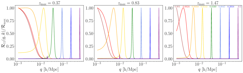
Figure 1: The kernel window function $\mathcal{R}_{11}(q,k)$ of Eq. (4.6) as a function of $q$, for seven values of $k$ selected to lie in the interval $k\in[0.001,0.5]\,h\,{\rm Mpc}^{-1}$, with the smallest in dark red and the largest in purple (see annotated values in the right-most plot). The panels from left to right show the results for volume limited surveys with maximum redshifts of $z_{\rm max}=\{0.37,0.83,1.47\}$, respectively, corresponding to a maximal radial distance of $\{1,2,3\}h^{-1}$Gpc in our chosen cosmology. We see that for scales much smaller than the survey volume the window functions take on Dirac delta function like behaviour: $\mathcal{R}_{11}(q,k)\approx\delta^{D}(q-k)$.

Figure 1 shows the behaviour of the kernel window function of Eq. (4.6), normalised by its maximum value. Here we present the case where there is no luminosity dependent galaxy bias, such that $b(L|r)=1$, and also for the linear theory UETC. We have also made the further simplifying assumption of a volume limited survey with a constant comoving number density of galaxies $n^{\rm LC}_{0}(r)=1$ up to a scale $r_{\rm max}$ and then a vanishingly small density thereafter. The three panels from left to right show the results for increasing survey volume. We see that on small scales (i.e. when $qr_{\rm max}\gg 1$ and $kr_{\rm max}\gg 1$) ${\mathcal{R}}$ becomes highly spiked and so exhibits delta function like behaviour where $k\approx q$. Not too unsurprisingly, this mimics the window function $G(k-q)$ described in the FKP method [28]. These plots demonstrate an important point, which is that when we compute $P_{\rm F}(q)$, to avoid wasting large amounts of computational time evaluating the $k$ integral in regions where the integrand is vanishingly small, we will make the bounds $q$ dependent.

4.2 The large-scale limit: $qr_{\rm max}\ll 1$

Let us consider the asymptotic limit of our full expression for the power spectrum observable given by Eq. (3.19) in the limit where $qr_{\rm max}\rightarrow 0$. In this case, we notice that

$$\lim_{qr_{\rm max}\rightarrow 0}j_{l}(qr)=\delta^{K}_{l,0}\ .$$ (4.8)

The consequence of this is that the sum over multipoles in Eq. (3.19) collapses and if we reorder the integrals so that the $k$-space integral is the innermost one, we see that we have:

$$\lim_{qr_{\rm max}\rightarrow 0}P_{\rm F}(q) =\prod_{a=1}^{2}\left\{A\int{\rm d}^{3}{\bf r}_{a}n^{\rm LC}_{\rm Eff}({\bf r}_{a})b^{\rm LC}_{\rm Eff}({\bf r}_{a})\right\}\Sigma(r_{1},r_{2})+P^{\rm LC}_{\rm shot},$$ (4.9)

where

$$\Sigma(r_{1},r_{2})\equiv\int\frac{{\rm d}^{3}{\bf k}}{(2\pi)^{3}}j_{0}(kr_{1})j_{0}(kr_{2})P(k,\eta_{1},\eta_{2})\ .$$ (4.10)

Consequently, the observed power spectrum on the past lightcone will asymptote to a constant amplitude on large scales. We have not seen this result derived elsewhere.

4.3 The small-scale limit: $qr_{\rm max}\gg 1$

Conversely, in the small-scale limit, where $qr_{\rm max}\gg 1$ we have seen from Figure 1 that the function ${\mathcal{R}}_{ab}(q,k)$ takes on the behaviour like that of Dirac’s delta function, such that ${\mathcal{R}}_{ab}(q,k)\propto\delta^{D}(k-q)$. If the functionals of the matter power spectrum ${\mathcal{F}}_{ab}[P(k,\eta_{0})](k)$ are slowly varying over the scale $q$, then we can write:

$$\lim_{qr_{\rm max}\rightarrow\infty}P_{\rm F}(q)\approx\sum_{ab}{\mathcal{F}}_{ab}[P(k,\eta_{0})](q)\int\frac{{\rm d}^{3}{\bf k}}{(2\pi)^{3}}\mathcal{R}_{ab}(q,k)+P^{\rm LC}_{\rm shot}\ .$$ (4.11)

Focusing on the last integral on the right-hand-side of the above expression we see that from Eqs (4.6) and (4.7) this is:

$$\int\frac{{\rm d}^{3}{\bf k}}{(2\pi)^{3}}\mathcal{R}_{ab}(q,k) =A^{2}\sum_{\ell}(2\ell+1)\int\frac{{\rm d}^{3}{\bf k}}{(2\pi)^{3}}$$

$$\times\prod_{\alpha=\{a,b\}}\left\{\int{\rm d}^{3}{\bf r}n^{\rm LC}_{\rm Eff}({\bf r})b^{\rm LC}_{\rm Eff}({\bf r})G_{\alpha}(\eta,\eta_{0})j_{\ell}(qr)j_{\ell}(kr)\right\}\ .$$ (4.12)

By expanding out the product, we see that we can reorder the integrals so that the $k$-integral is computed first. On recalling the orthogonality relation of the spherical Bessel functions,

$$\int\frac{{\rm d}^{3}{\bf k}}{(2\pi)^{3}}j_{\ell}(kr_{1})j_{\ell}(kr_{2})=\frac{1}{4\pi r_{2}^{2}}\delta^{D}(r_{1}-r_{2})\ ,$$ (4.13)

we see that the integral over $r_{2}$ can be done trivially to yield:

$$\int\frac{{\rm d}^{3}{\bf k}}{(2\pi)^{3}}\mathcal{R}_{ab}(q,k) =A^{2}\int{\rm d}^{3}{\bf r}\left[n^{\rm LC}_{\rm Eff}({\bf r})b^{\rm LC}_{\rm Eff}({\bf r})\right]^{2}G_{a}(\eta,\eta_{0})G_{b}(\eta,\eta_{0})\sum_{\ell}(2\ell+1)j_{\ell}^{2}(qr)$$

$$=A^{2}\int{\rm d}^{3}{\bf r}\left[n^{\rm LC}_{\rm Eff}({\bf r})b^{\rm LC}_{\rm Eff}({\bf r})\right]^{2}G_{a}(\eta,\eta_{0})G_{b}(\eta,\eta_{0})\ ,$$ (4.14)

where the final equality in the above expression follows from the fact that an infinite sum over the squares of spherical Bessel functions is unity [53, result 10.1.50]:

$$\sum_{\ell}^{\infty}(2\ell+1)j^{2}_{\ell}(x)=1\ .$$ (4.15)

Thus we see that Eq. (4.11) tends to the form:

$$P_{\rm F}(q) \approx A^{2}\sum_{ab}{\mathcal{F}}_{ab}[P(k,\eta_{0})](q)\int{\rm d}^{3}{\bf r}\left[n^{\rm LC}_{\rm Eff}({\bf r})b^{\rm LC}_{\rm Eff}({\bf r})\right]^{2}G_{a}(\eta)G_{b}(\eta)+P^{\rm LC}_{\rm shot}$$

$$\approx A^{2}\int{\rm d}^{3}{\bf r}\left[n^{\rm LC}_{\rm Eff}({\bf r})b^{\rm LC}_{\rm Eff}({\bf r})\right]^{2}P(q,\eta)+P^{\rm LC}_{\rm shot}\ .$$ (4.16)

By making an appropriate choice for $A$, for example

$$\frac{1}{A^{2}}\equiv\int{\rm d}^{3}{\bf r}\left[n^{\rm LC}_{\rm Eff}({\bf r})\right]^{2}\ ,$$ (4.17)

we see that in the limit where the the radial weight functions are very broad and smooth, such that the $W_{\ell}^{(a)}(q,k)$ are very narrowly peaked, the lightcone power spectrum is approximately given by the equal time correlator weighted by the square of the selection function averaged over the radial extent of the survey. We note that this result for the small-scale limit agrees with that found by [22] (see their Eq (16)). However, we note that how we take the limit differs in detail, owing to the differences in our final expressions $P_{\rm F}(q)$.

Figure 2: Upper: A plot of the window-convolved nonlinear power spectrum on the lightcone for an all sky survey reaching out to increasing redshift depths (corresponding to brighter magnitude cuts). The solid lines show the unequal time model (Eq. (4.5)), while the dot-dashed lines show the small scale approximation (Eq. (4.16)). The lower plot shows the percentage difference between calculating the power spectrum using the full formula versus using the small scale approximation. We see that these two formulas reach convergence to well within $1\%$ on small scales, where the approximate formula is used to reduce computation time.

In Figure 2 we plot the window-convolved power spectrum on the past lightcone for an all-sky survey, out to increasing redshift depths, using the full expression of Eq. (4.5) (solid lines). We also plot the small-scale approximation given by Eq. (4.16) with the dash-dotted lines, with the lower panel of the plot showing the percentage difference between the two methods. We see that for the cases considered, for $q>0.1\,h\,{\rm Mpc}^{-1}$, there is $\lesssim 1\%$ difference between the two formulae, and so in this region we can safely use the approximated formula, which will drastically save on computational time. We also see that the approximation performs worse for shallower survey depths, where one has to calculate the full formula to a higher value of $k$, relative to a deeper survey, before being able to safely switch over to this approximation.

4.4 Evaluating theoretical models at a fixed time

In many large-scale structure analyses, it is common to find that the theoretical models are evaluated at the mean redshift of the sample, calculated via :

$$z_{\mathrm{mean}} =\frac{\int{\rm d}z({\rm d}V/{\rm d}z)\;z\;n^{\rm LC}_{\rm Eff}(z)b^{\rm LC}_{\rm Eff}(z)}{\int{\rm d}z({\rm d}V/{\rm d}z)\;n^{\rm LC}_{\rm Eff}(z)b^{\rm LC}_{\rm Eff}(z)}\ .$$ (4.18)

Alternatively, one can instead use an effective survey-fixed redshift. On inspection of Eq. (4.5) we see that, for a general nonlinear model, this can not be realised in detail and that the presence of nonlinear terms with different time dependence violates this approximation. To emphasise this point more completely, let us work with the observed power spectrum in the small-scale limit approximation of §4.3 given by Eq. (4.16). Let us take this simplified form and, neglecting shot-noise, assume that there is an effective time at which we have the following equality:

$$P_{\rm F}(q)\approx\int{\rm d}^{3}{\bf r}w(r)P(q,\eta)\stackrel{{\scriptstyle?}}{{\approx}}P(q,\eta_{\rm eff})\ ,$$ (4.19)

where $w(r)=A^{2}\left[n^{\rm LC}_{\rm Eff}({\bf r})b^{\rm LC}_{\rm Eff}({\bf r})\right]^{2}$ and a super-script question notates that we are asking whether the conjecture is true. On making repeated use of Eq. (4.1) we find:

$$\sum_{a,b}\int{\rm d}^{3}{\bf r}w(r)G_{a}(\eta,\eta_{0})G_{b}(\eta,\eta_{0}){\mathcal{F}}_{ab}[P(k,\eta_{0})](k)\stackrel{{\scriptstyle?}}{{\approx}}\sum_{a,b}G_{a}(\eta_{\rm eff},\eta_{0})G_{b}(\eta_{\rm eff},\eta_{0}){\mathcal{F}}_{ab}[P(k,\eta_{0})](k)$$ (4.20)

For the case of linear theory, where $a=1$, $b=1$, $G_{1}(\eta,\eta_{0})=D(\eta,\eta_{0})$ and ${\mathcal{F}}_{ab}[P(k,\eta_{0})](k)=P_{\rm Lin}(k,\eta_{0})$, we see that a ‘Linear’ effective time $\eta_{\rm eff}^{\rm Lin}$ can be found that will satisfy Eq. (4.20) if we can numerically solve the relation:

$$D^{2}(\eta_{\rm eff}^{\rm Lin})=\frac{\int{\rm d}^{3}{\bf r}\left[n^{\rm LC}_{\rm Eff}({\bf r})b^{\rm LC}_{\rm Eff}({\bf r})\right]^{2}D^{2}(\eta,\eta_{0})}{\int{\rm d}^{3}{\bf r}\left[n^{\rm LC}_{\rm Eff}({\bf r})b^{\rm LC}_{\rm Eff}({\bf r})\right]^{2}}\ .$$ (4.21)

We note that this result is related, but not identical, to the effective redshift noted in [44]. However, what is now also clear, is that as soon as we add in any additional nonlinear terms, they would obey a different set of equations. Hence, we conclude that there is no effective time which would satisfy both the linear and nonlinear evolutionary terms allowing for a single effective time.

We can get an idea of the error that is incurred by making the unique time approximation by considering the case of standard perturbation theory at the 1-loop level. In this case, if we set $\eta_{\rm eff}$ in accordance with Eq. (4.21), then the first term in the left-hand and right-hand-side expansions of Eq. (4.20) are guaranteed to vanish. The next terms which come from the loop corrections would thus incur the error:

$$P_{\rm Err}(k,\eta_{\rm eff}^{\rm Lin}) =\left[P_{13}(k,\eta_{\rm eff}^{\rm Lin})+P_{22}(k,\eta_{\rm eff}^{\rm Lin})\right]$$

$$\times\left\{1-\frac{\int{\rm d}^{3}{\bf r}\left[n^{\rm LC}_{\rm Eff}({\bf r})b^{\rm LC}_{\rm Eff}({\bf r})\right]^{2}[D(\eta)/D(\eta_{\rm eff}^{\rm Lin})]^{4}}{\int{\rm d}^{3}{\bf r}\left[n^{\rm LC}_{\rm Eff}({\bf r})b^{\rm LC}_{\rm Eff}({\bf r})\right]^{2}}\right\}\ .$$ (4.22)

If one could guarantee that, on a given scale, a nonlinear correction of a certain order was dominant, then one could find a new effective time to evaluate the theory at. For example, if there is a scale where the 1-loop contribution is dominant and the linear and 2-loop corrections are negligible, then one could evaluate the theory at the 1-loop effective time, $\eta_{\rm eff}^{\rm 1-loop}$, defined through solving the relation:

$$D^{4}(\eta_{\rm eff}^{\rm 1-loop})=\frac{\int{\rm d}^{3}{\bf r}\left[n^{\rm LC}_{\rm Eff}({\bf r})b^{\rm LC}_{\rm Eff}({\bf r})\right]^{2}D^{4}(\eta,\eta_{0})}{\int{\rm d}^{3}{\bf r}\left[n^{\rm LC}_{\rm Eff}({\bf r})b^{\rm LC}_{\rm Eff}({\bf r})\right]^{2}}\ .$$ (4.23)

Iterating on this logic, one would thus need a set of effective times for all the scales where the various nonlinear components dominate the clustering signal.

To compare these fixed-time approximations to the full unequal-time correlator model, we have assumed the simple case of no weights such that $w(L,r)=1$, but have modelled the linear bias as evolving, using the Generalised Time Dependent (GTD) model of [54]:

$$b^{\rm LC}_{\rm Eff}({\bf r})=c+\frac{b_{0}-c}{D^{\mu}(r)}\ .$$ (4.24)

By making the parameter choices of $c=0.58$, $b_{0}=0.83$ and $\mu=2.23$, this function very accurately represents the widely used model of bias found in [55], which is calibrated using a wide range of $N$-body simulations. For modelling the number density on the light cone, $n^{\rm LC}_{\rm Eff}({\bf r})$, we use an evolving Schechter function which we discuss further in §5.3.

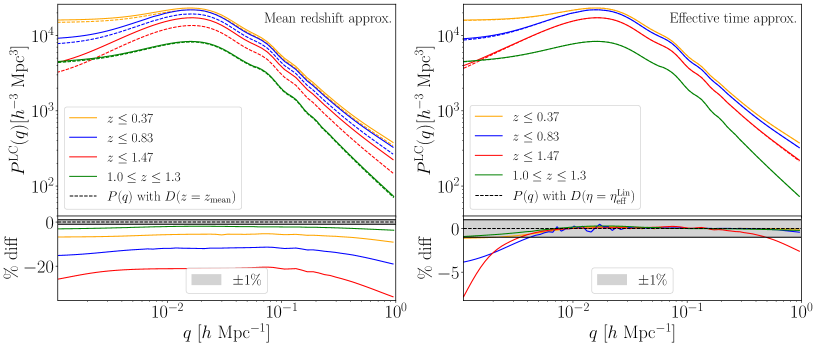
Figure 3: Theoretical predictions of the mater power spectrum on the lightcone, as a function of wavenumber for full-sky surveys of different depths (see plot legend). Left upper panel: Comparison of the full calculation of Eq. (4.5) (with the nonlinear UETC model) with the mean redshift approximation of Eq. (4.18), where the power spectrum is evaluated with the growth factor fixed at $D(z=z_{\rm mean})$. The solid lines represent the full calculation and the dashed lines the approximation. Right upper panel: same as left panel, except the comparison is with the effective time approximation $D(\eta=\eta_{\rm eff}^{\rm Lin})$ from Eq. (4.21). The lower section of each panel shows the percentage difference between the full calculation and the approximation. The shaded region shows $\pm 1\%$ deviation.

In Figure 3 we illustrate the impact of using the different approaches to a fixed-time approximation. In both of the plots, we show the unequal-time power spectrum model (solid lines) for increasing survey depth. This is calculated using Eq. (4.5) on large scales, and uses the small-scale approximation of Eq. (4.16) for scales well within the scale of the survey window function. In the left hand plot, we compare this with the mean redshift approximation of Eq. (4.18), and in the right hand plot we instead use the effective redshift (or time) approximation calculated from Eq. (4.21), with both approximations represented by dashed lines. The lower plots in each case show the percentage difference between the full model and the given approximation, with the shaded region showing the $\pm 1\%$ threshold. We see that using the mean redshift approximation results in a $k$-dependent bias of the power spectrum amplitude, which increases with severity as the survey depth increases. At intermediate scales where there is minimal convolution with the survey window function and non-linear effects are small, this offset is roughly constant due to the fact that the linear power spectrum scales as $D^{2}(r)$. We notice that the difference grows larger at smaller scales where we pick up non-linear corrections, depending on higher powers of the growth factor. Conversely, from the right hand plot, we see that using the effective time approximation works very well at all but the largest and smallest scales, only deviating from sub-percent level accuracy at these extremities for the deeper survey examples. Therefore, where a fixed time approximation is required to evaluate theory, we strongly advocate the use of Eq. (4.21) to do this.

4.5 Extending the theory to the nonlinear regime

Building on the analysis of the previous sections, it is now straightforward to extend our model for the power spectrum in the small-scale limit to the non-linear regime. We do this by perturbatively expanding the density field in terms of powers of the square of the growth factor. Using the approximate form of Eq. (4.16), we now substitute in the equal-time version of the UETC expansion of the density field from Eq. (4.3), and up to ‘2-loops’ this, gives us:

$$P_{\mathrm{F}}(q) \approx P_{\mathrm{Lin}}(q)\mathcal{W}^{(2)}+P_{\mathrm{1-loop}}(q)\mathcal{W}^{(4)}+P_{\mathrm{2-loop}}(q)\mathcal{W}^{(6)},$$ (4.25)

where for brevity we have made the definition:

$$\mathcal{W}^{(i)}\equiv A^{2}\int{\rm d}^{3}{\bf r}\left[n^{\rm LC}_{\rm Eff}({\bf r})b^{\rm LC}_{\rm Eff}({\bf r})\right]^{2}D^{i}(r)\ .$$ (4.26)

In summary, our final model for the power spectrum on the past lightcone is a piecewise combination of two different models: on large scales, we use the full expression of Eq. (4.5) with the 1-loop UETC model of Eq. (4.3), and on small scales, we use the approximation of Eq. (4.25). Furthermore, we use CAMB to generate the linear theory $P_{\mathrm{Lin}}$, and then FAST-PT [56], with $P_{\mathrm{Lin}}$ as input, to generate the 1-loop terms. Finally, to calculate a proxy for the ‘2-loop’ terms we compute the nonlinear power spectrum model of [57], and subtract off $P_{\mathrm{Lin}}$ and the 1-loop contribution from FAST-PT. These are all generated at $z=0$ and then scaled as appropriate using powers of the growth factor $D^{i}(r)$ as indicated above.

5 Validation with $N$-body simulation mock catalogues

We now turn to the issue of validating the derived expressions using galaxy mock catalogues obtained from $N$-body simulations of the past lightcone. We first detail the $N$-body data that we use, the process for creating the dark matter lightcones, and then finally the estimator methodology that we use to measure the power spectrum.

5.1 Dämmerung Simulation

To generate past lightcones we make use of the large-volume simulation from the “Dämmerung Suite” of runs [for details see 58], which allows us to measure the power spectrum over a wide range of scales. In summary, the cosmological parameters of this run were in accord with the Planck best-fit [59]. The exact cosmological parameter values that were used are: the dark energy equation of state parameters were $w_{0}=-1.0$ and $w_{a}=0.0$; the dark energy density parameter was $\Omega_{\rm DE}=0.6914$, which, since the cosmological model was spatially flat gave a matter density $\Omega_{\rm m}=0.3086$; the physical densities of cold dark matter and baryons were set to $\omega_{c}=0.11889$ and $\omega_{b}=0.022161$, respectively; the primordial power spectrum spectral index, amplitude and running were set to $n_{\rm s}=0.9611$, $A_{s}=2.14818\times 10^{-9}$ and $\alpha=0.0$, respectively. The linear matter power spectrum was computed using CAMB [60], down to $z=0$. This was rescaled back to the $z=49$ using the scale-independent matter only linear growth factor and the initial conditions were lain down using an upgraded version of 2LPT [61].

The simulation was run using the Gadget-3 code developed for the Millennium-XXL simulation[62, 63]. The large-volume run was performed with $N=2048^{3}$ dark matter particles, in a comoving box of size $L=3000\,h^{-1}{\rm Mpc}$, yielding a mass per particle of $m_{\rm p}=2.69\times 10^{11}\rm{h^{-1}M_{\odot}}$. Sixty snapshots were output between $z=49$ and $z=0$, with a hybrid linear-logarithmic output spacing that matched the Millennium Run I simulation [64]. The simulation was run on the SuperMUC machine at the Leibniz Rechnum Zentrum in Garching and the full particle data storage was $\sim$20 TB.

5.2 Construction of the past lightcones for dark matter particles

Full details of our method for construction of the past lightcone will described separately in Booth et al. (in prep.), but the basic methodology follows the work of [65], differing though in the details. The main steps of the algorithm can be summarised as follows:

• We wish to solve the lightcone crossing equation for each dark matter particle in the $N$-body simulation. Concretely, for the $k$th particle we want find the value of $t^{\rm c}$ that satisfies the equation

  $$\left|{\bf r}_{k}(\chi,\theta,\phi,t^{\rm c})-{\bf r}_{\mathcal{O}}\right|=\int^{t_{0}}_{t^{\rm c}}\frac{cdt}{a(t)}\ ,$$ (5.1)

  where ${\bf r}_{k}$ is the worldline of the particle, ${\bf r}_{\mathcal{O}}$ is the observers location and $t^{\rm c}$ gives the coordinate time when the particle exits the past lightcone.

• In order to solve the above equation, we need to reconstruct the full world line of each particle. We do this in a piece wise fashion by using a Taylor expansion up to cubic order in lookback time to interpolate the particle positions and velocities between neighbouring snapshots. The parameters of the Taylor expansion are fixed using the particle positions and velocities at the snapshots. For example, the equation for the Cartesian $x$ component of the particle world line is:

  $$x(t) \approx\overline{X}-\frac{\Delta V\Delta T}{8}+\frac{\left(3\Delta X-\overline{V}\Delta T\right)}{2}\left(\frac{t-\overline{T}}{\Delta T}\right)+\frac{\Delta V\Delta T}{2}\left(\frac{t-\overline{T}}{\Delta T}\right)^{2}$$

  $$-2\left[\Delta X-\overline{V}\Delta T\right]\left(\frac{t-\overline{T}}{\Delta T}\right)^{3};$$ (5.2)

  where $\overline{T}\equiv(t_{i}+t_{i+1})/2$ and where $\Delta t=t-\overline{T}_{i}$ with $t_{i}$ and $t_{i+1}$ being the lookback times to the neighbouring snapshots, with $t_{i}<t_{i+1}$. Also we have defined $\overline{X}\equiv(x_{i}+x_{i+1})/2$, $\Delta X\equiv x_{i+1}-x_{i}$, $\overline{V}\equiv(v_{i+1}+v_{i})/2$, and $\Delta V\equiv v_{i+1}-v_{i}$, with $(x_{i},v_{i})$ and $(x_{i+1},v_{i+1})$ referring to the particle’s position and velocity for the neighbouring snapshots, respectively. In Booth et al. (in prep.) we show that for our simulation we can do this to an accuracy of $r\lesssim 200\,h^{-1}{\rm kpc}$, for all particles.

We apply the above algorithm to generate 8 different dark matter particle light cones, where we have set the different observer locations to be the vertices of a cubical lattice of side $L/2=1500\,h^{-1}{\rm Mpc}$. The data footprint of each particle light cone is roughly $\sim 2$TB. While these ligtcones are not fully independent, on scales smaller than $r\lesssim L/4$ they have no repeated structures and thus for shallower surveys can be considered independent from one another. The further advantage of doing this for the deeper lightcones is that one averages over similar structures, but at different epochs. Nevertheless, in what follows while we will present the mean statistic averaged over the 8 quasi-independent light cones, we will compute the errors on the observables using the Gaussian theory estimates.

5.3 Constructing the galaxy past lightcone

We would like to be able to explore how well the theory from the previous sections works for a galaxy sample that would be comparable to that for the Bright Galaxy Sample (hereafter BGS-like) from DESI or the 4MOST Cosmology Redshift Survey. Owing to the fact that the large-volume “Dämmerung run” does not have sufficient resolution to resolve the typical halo masses in these surveys, we adopt the simplified strategy of assuming that the BGS-like galaxies are a Poisson sampling of the dark matter particles (i.e. are unbiased). However, we do introduce realistic radial selection functions to emulate the effects of the flux-limits that we adopt. Our mock galaxy recipe follows the following steps:

1. Adopt a magnitude limit, $m_{\rm lim}$, and set bounding redshifts $z_{\rm min}$ and $z_{\rm max}$ for the survey.

2. Next, we assume an (evolving) galaxy luminosity function (GLF) for the survey. The number density of particles in the dark matter past lightcone sets the maximum density of galaxies in the mock catalogue, such that:

   $$\bar{n}_{\rm max}(r)\geq\int_{\rm L_{\rm min}(r)}^{\infty}\phi(L,r){\rm d}L\ ,$$ (5.3)

   where $\phi(L,r)$ is the evolving GLF, and in our case we follow the work of [66] and use a Schechter function form:

   $$\phi(L,r){\rm d}L=\phi^{*}(r)\left(\frac{L}{L^{*}(r)}\right)^{\alpha}\exp\left(-\frac{L}{L^{*}(r)}\right)\frac{{\rm d}L}{L^{*}(r)}\ ,$$ (5.4)

   where the parameters $\phi^{*}(r)$ and $L^{*}(r)$ evolve as a function of radial comoving distance and $\alpha$ is fixed for all redshifts (for full details see Appendix C.1). Thus for a given $\bar{n}_{\rm max}$ we see that this imposes the minimum luminosity that a galaxy could have and still make it into the survey.

3. To each dark matter particle in the lightcone we now sample a luminosity from the GLF following the methodology outlined in Appendix C.2.

4. For the specified flux-limit, and for a given particle with redshift $z$, we then use Eq. (B.5) to determine the minimum luminosity that a galaxy could have at that distance and be contained in the survey. This step is most efficiently done through creating a cubic-spline of this function. We then include or exclude the potential mock galaxy (particle) based on whether its luminosity satisfies $L\geq{L_{\rm min}}(r)$.

5. Finally, this process is repeated for all of the flux-limit samples of interest.

We take 5 magnitude cuts at $m_{\rm{lim}}=\{18,19,20,21,22\}$ (see Appendix §C.2 for details on sampling). We note that these catalogues are thus not independent realisations from one another, but rather the faintest catalogue, $m_{\rm{lim}}=18$, contains a subset of particles from the $m_{\rm{lim}}=19$ catalogue, which in itself is a subset of the $m_{\rm{lim}}=20$ catalogue, and so on.

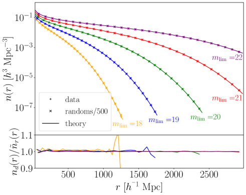
Figure 4: Evolution of the mean galaxy density as a function of the comoving distance. Upper panel: the galaxy number densities measured from the mock are shown by the plus symbols, the crosses show the same but for the random catalogue scaled by $1/R_{\rm multi}$. Different colours indicate the different magnitude limits. The solid lines represent the theoretical prediction from integrating the evolving Schechter function, as in Eq. (C.1). Lower panel: the ratio of the number densities measured in the mock data with that of the random distributions down weighted by $R_{\rm multi}$.

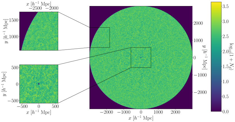
Figure 5: Cross section slice through the centre of the full-sky dark matter lightcone, including zoom regions near the edge and the centre of the sphere. The cross section is $40\,\,h^{-1}{\rm Mpc}$ thick and spans a redshift range of $z=0$ at the centre to $z\approx 1.45$ at the outer edge. The heatbar at the right shows the logarithm to base ten of the particle number per pixel.

We also generate unclustered mock random data sets to go alongside these magnitude-cut catalogues, for use in our power spectrum measurements. These random catalogues are created by distributing points uniform-randomly in a sphere of radius $r_{\rm{max}}=3$ $h^{-1}$Gpc, and then sampling magnitudes using the same method as above and making matching apparent magnitude limit cuts – one small difference though, is that we omit Step ii and use the same $L_{\rm min}(r)$ as the clustered catalogue to sample luminosities with. This process is iterated for each cut, until we have 5 mock random catalogues, which match the overall survey geometry of their data counterparts, but with $N_{\rm{rand}}=R_{\rm multi}N_{\rm{data}}$ for each. In our case, we set $R_{\rm multi}\simeq 500$, choosing this high value to reduce the probability of any bias or random error. Table 1, presents some of the key details of our full sky dark matter lightcone and the details of our 5 flux-limited mock galaxy catalogues, averaged over the 8 realisations.

Figure 4 shows the resultant number densities of the different mock galaxy catalogues for both the data and the randoms. Here we also show the expected theoretical prediction given by Eq. (C.1) as the solid lines and as can be seen the mock and random catalogues and the theory have exactly the same evolution with comoving radial distance.

Figure 5 shows a slice through one of the full-sky dark matter lightcones and several zoom-in regions. These panels visually demonstrate how the clustering of the large-scale structure drops off as on goes from the inner ring to outer rim of the lightcone sphere.

$m_{\rm lim}$	Avg. $N_{d}$	$z$ range	$\chi$ range [$h^{-1}{\rm Mpc}$]
None	$35.0\times 10^{9}$	$0.01\leq z\leq 1.45$	$30\leq\chi\leq 2974$
18.0	$4.6\times 10^{6}$	$0.01\leq z\leq 0.36$	$30\leq\chi\leq 975$
19.0	$16.7\times 10^{6}$	$0.01\leq z\leq 0.53$	$30\leq\chi\leq 1390$
20.0	$60.0\times 10^{6}$	$0.01\leq z\leq 0.81$	$30\leq\chi\leq 1950$
21.0	$212.8\times 10^{6}$	$0.01\leq z\leq 1.24$	$30\leq\chi\leq 2680$
22.0	$756.0\times 10^{6}$	$0.01\leq z\leq 1.45$	$30\leq\chi\leq 2974$

Table 1: List of mock galaxy lightcones. Column 1, gives the apparent magnitude cut (the case where no limit is taken gives the dark matter lightcone); column 2 gives the galaxy/particle count $N_{d}$ averaged over the 8 realisations; column 3 gives the ‘effective’ redshift range; and column 4 the corresponding comoving distance. Note that the upper bound of these ranges signifies where $n(r)$ drops 4 orders of magnitude below its peak value, where it is $\leq 2974h^{-1}{\rm Mpc}$ (see Fig. 4).

5.4 The power spectrum estimator

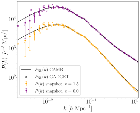
Figure 6: Validation of the matter power spectrum $P(k)$ estimates from the Dämmerung simulation snapshots as a function of wavenumber. The orange and purple symbols show the results from snapshots $z=1.5$ and $z=0$, respectively. The solid circles show the results from our estimator. The crosses represent the output from the GADGET-4 code. The black solid lines show the nonlinear $P(k)$ predictions from CAMB.

To estimate the power spectra from each catalogue, we broadly follow the FFT based method of [28] and [67], but with some small variations, which we summarise below.

• First, both the mock data and random catalogues were interpolated onto a cubical mesh of dimension $N_{\rm grid}=1024^{3}$, using the Triangular-Shaped-Cloud (TSC) mass assignment scheme [68]. The cubical mesh was selected to be large enough to contain the diameter of the dark matter light cone.

• We then implemented the estimator of [67] in Python 3.6 (Python Software Foundation, https://www.python.org/), making use of NumPy [69], SciPy [70], AstroPy [71], Numba [72], and the python wrappers for MPI [73] and FFTW [74].

• To reduce the effects of small-scale aliasing caused by the finite resolution of the grid [see 75, for a discussion], we employed the interlacing method of [76]. In that work, it was demonstrated that, through combining the TSC assignment with interlacing, one is able to measure the power spectrum in a periodic box to $\lesssim 0.1\%$ accuracy all the way up to the Nyquist frequency of the grid ($k_{\rm Ny}=\pi N_{\rm grid}/L$).

• For the covariance, we took Eqn (20) from [67]:

  $$\left<\delta P({\bf k}_{i})\delta P({\bf k}_{j})\right>=\frac{2A^{4}\sum_{{\bf k}_{i},{\bf k}_{j}}|P({\bf k}_{i})Q({\bf k}_{i}-{\bf k}_{j})+S({\bf k}_{i}-{\bf k}_{j})|^{2}}{N_{{\bf k}_{i}}N_{{\bf k}_{j}}},$$ (5.5)

  where $N_{{\bf k}_{i}}$ is the number of modes in a given bin and the equations for $Q({\bf k})$ and $S({\bf k})$ are given by:

  $$Q({\bf k}) =\sum W^{2}({\bf x})w^{2}({\bf x})\exp(i{\bf k}\cdot{\bf x})\ ;$$ (5.6)

  $$S({\bf k}) =\sum W({\bf x})w^{2}({\bf x})\exp(i{\bf k}\cdot{\bf x})\ .$$ (5.7)

It is worth pointing out that while we have assumed that the underlying Fourier modes of the galaxy density field are Gaussianly distributed, Eq. (5.5) shows that the observed power spectrum in different $k$-bins does become correlated, due to the the survey window function. However, in the limit that the survey window function is sufficiently compact, centred on each bin, we see that the diagonal covariance approximation will be accurate on scales that lie sufficiently within the survey. For larger scales though, this will be an under-estimate. The former case leads to the following approximate form for the covariance (FKP Eqn. (2.2.6)):

$$\left<[\delta P({\bf k}_{i})]^{2}\right>\simeq\frac{2A^{4}}{N_{{\bf k}}}|P({\bf k}_{i})Q({\bf k}_{i})+S({\bf k}_{i})|^{2}.$$ (5.8)

To test the accuracy of the code, we first applied it to measure the power spectrum of the original Dämmerung Simulation redshift snapshots, where our results can easily be compared to the output of CAMB nonlinear power spectra at the specified redshift, as well as the power measured by GADGET-4 [77]. We perform the measurements in 25 logarithmically spaced bins, where the upper and lower bin edges are set to match the largest and smallest modes supported by the box, giving bin edges such that $0.0021\,h\,{\rm Mpc}^{-1}\leq k\leq 1.07\,h\,{\rm Mpc}^{-1}$, and bin width $\log_{10}(\Delta k/[\,h\,{\rm Mpc}^{-1}])=0.108$.

Figure 6 presents the results from these tests, where we measure the power spectrum at redshifts $z=0.0$ and $z=1.5$, which is the approximate redshift range spanned by our lightcone simulations. We see excellent agreement between our measurements and the nonlinear prediction from CAMB and GADGET across all scales. At the largest scales, just beyond the turnover scale, we see a slight increase in power relative to the linear theory. This we attribute to cosmic variance. As we will in the next section, this noise feature is also present in the lightcone measurements. Note that the error bars are based on Eq. (5.8) and that we have computed the spectrum all the way to the Nyquist frequency of the Fourier mesh with no resultant boost in power, characteristic of aliasing effects. This gives us confidence that the estimator methodology is working as desired, and we now move on to tackle the analysis of the lightcone data.

6 Results: power spectrum on the past lightcone

6.1 Measurements of the mock lightcone survey catalogues

We now measure the power spectrum for the 8 pseudo-independent realisations of our lightcone, in the 5 different apparent magnitude limited mock galaxy catalogues. This gives us a total of 40 sets of measurements to perform. As with our testing on the individual Dämmerung snapshots, we measure the power in 25 logarithmically spaced bins, but this time with $k$-range of $0.0042\,h\,{\rm Mpc}^{-1}<k\leq 0.54\,h\,{\rm Mpc}^{-1}$. This gives a $k$-bin width of $\log_{10}(\Delta k/[\,h\,{\rm Mpc}^{-1}])=0.0844$. The reduction in the upper wavemode cut-off is due to the fact that the length of the cubical box being twice the size of the original Dämmerung Simulation box. The effect of which is to halve the Nyquist frequency. In addition, we set the lowest frequency bin to be twice the fundamental mode of the base simulation $k_{\rm f}=2\pi/(1500h^{-1}\rm{Mpc})\approx 0.0042\,h\,{\rm Mpc}^{-1}$. For wavemodes below this scale mode discreteness and the box replication is relevant and we would expect repeated structures to appear on the same lightcone, despite their ‘existing’ at different epochs.

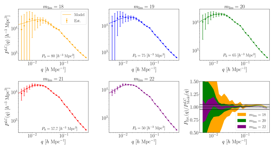
Figure 7: Upper and left: Plots of the FKP-weighted power spectrum measurements (points with error bars) from the 5 different magnitude cut catalogues, compared with the predictions from the theory (solid line). Bottom right: Ratio plots comparing the measurements to the model for 3 of the catalogues, with 5% difference in the shaded grey region.

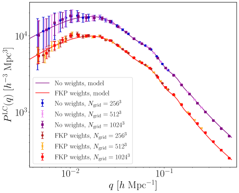
Figure 8: Plot showing the effect of varying the grid resolution on the power spectrum measurements. We show estimates from using $256^{3}$, $512^{3}$ and $1024^{3}$ FFT grids, for both unweighted (blue hues) and FKP weighted (red hues) data, using the $m_{\rm lim}=22$ catalogue, as well as the theoretical predictions (solid lines). Aside from a different available $k$ range of measurements, we see that grid resolution has little effect on the resulting measured power. Note that weighed measurements and model have been offset by a factor of $0.7$ in the vertical direction for clarity.

Figure 7 shows the galaxy power spectra measurements, averaged over the 8 realisations for each of the 5 magnitude cuts. The error bars are computed from Eq. (5.8) and the solid line shows the theoretical prediction using the recipe described in §3. For this set of measurements we have employed an FKP weighting scheme where the choice of $P_{0}$ is indicated in the text box on each plot, and is chosen to match the approximate magnitude of the overall shot-noise contribution. We found that setting $P_{0}\gtrsim 10^{3}h^{-3}\,{\rm Mpc}^{3}$ introduced some bias to the shape of the power spectrum estimator at both the small and large scales. We believe that this may be caused by the optimal weights being applied as a grid based operation and not at the particle level at the point of applying the particles to the mesh. However, we note that [78] showed that variations in $P_{0}$, and therefore the weighting functions, would lead to a shape dependence of the power spectrum on the largest of scales. We reserve further investigation of this issue for future work.

The bottom right subplot of the figure shows the ratio between the measurements and the theory. The shaded regions denote the 1-$\sigma$ error envelopes for the $m_{\mathrm{lim}}=\{18,20,22\}$ catalogues, respectively. In this plot we also show the $\pm 5\%$ difference between theory and measurement as the shaded grey horizontal region. For all of the magnitude cuts, we see that the theory lies well within the error bars of the measurements at all scales, right up to the Nyquist frequency of the grid. We do see some slight fall off of the estimated power for scales of around $k\geq 0.2\;[h\;\mathrm{Mpc}^{-1}]$. This is most likely due to inaccuracies of our modelling of the 2-loop corrections to the theory as detailed in §4.5.

6.2 FFT grid resolution tests

Owing to the fact that our full-sky lightcones are non-periodic functions, it is interesting to examine whether there is any impact of grid-resolution, and thus, aliasing effects on the estimated power spectra. We examine this by focusing our attention on the deepest $m_{\rm lim}=22$ galaxy catalogue and fixing the weighting scheme and varying the FFT grid dimension.

Figure 8 shows the results of this exercise for the three grid resolutions $N_{\rm grid}=256^{3}$, $512^{3}$ and $1024^{3}$ and for the case of equal weights and FKP weights, with $P_{0}=100h^{-3}\rm{Mpc}^{3}$. We see that the estimates for the different grid resolutions are in excellent agreement, showing a close grouping for both the weighted and unweighted cases. We also show again our theoretical predictions from §3.2 for the case of the equal weight and FKP weighting. These results indicate that the small-scale discrepancies, noted earlier, are most likely caused by issues with the nonlinear modelling, as opposed to any effects from aliasing or the interlacing with the TSC charge assignment.

7 The turnover scale as a probe of the epoch of matter-radiation equality

7.1 Modelling the turnover scale

As an application of our formalism and mock galaxy catalogue development, we turn to the question of detecting the turnover scale of the matter power spectrum. One of the exciting aspects of being able to measure the power spectrum on very large scales is that it presents us with the opportunity to probe the epoch of matter-radiation equality in the early universe. The imprint of this epoch can be directly linked to the peak of the power spectrum: the theory of inflation predicts that the primordial matter power spectrum should follow a simple power-law of the form, $P_{\rm primordial}(k)\propto k^{n_{\rm s}}$ on very large scales. However, as the Universe expands from a hot-dense state, fluctuation growth inside the horizon is suppressed by radiation pressure support and radiation dominated expansion – this effect is commonly termed the ‘Mézáros Effect’ [for a detailed treatment see 79]. The consequence of this is that the peak point of the power spectrum, located at $k_{0}$, corresponds to the size of the cosmological horizon at the epoch of matter-radiation equality, and its measurement thus allows us to constrain the redshift of this epoch. This in turn is sensitive to both the matter density and Hubble parameters through the combination $\Omega_{m}h^{2}$, amongst other parameters.

To explore the detectability of this scale we broadly follow the work of [49]. This was subsequently refined by [80], who applied the process to the WiggleZ Dark Energy Survey to measure the parameters $\{k_{0},z_{\mathrm{eq}},\Omega_{m}h^{2}\}$. We refer the reader to these papers for full details. Here we model the power spectrum at its peak as two piecewise power laws of the form:

$$\log_{10}P(k) =\begin{cases}\log_{10}\big{[}P_{0}(1-\alpha x^{2})\big{]}&\text{if $k_{0}>k$},\\ \log_{10}\big{[}P_{0}(1-\beta x^{2})\big{]}&\text{if $k_{0}\leq k<k_{\rm max}$},\end{cases}$$ (7.1)

where

$$x\equiv\frac{\ln k-\ln k_{0}}{\ln k_{0}},$$ (7.2)

$P_{0}$ is the power spectrum amplitude at turnover, and $\alpha$ and $\beta$ are parameters that define the slope of the power spectrum on either side of the turnover [for an alternate approach that employs a logarithmic power-law see 81].

7.2 Parameter estimation and feature detectability

We now examine how well one could detect the turnover scale $k_{0}$ from flux-limited full-sky, galaxy redshift surveys. We fit the above model to three different sets of power spectra data:

• Case 1: $P(k)$ measured from magnitude limited mocks, with equal weights (see §5).

• Case 2: same as case 1, but where each galaxy is weighted by the FKP weight.

• Case 3: $P(k)$ are the theoretical predictions (given by the solid lines in Fig. 7). In this case the error bars are estimated from the actual measurements. We use this latter case to better assess biases and the impact of cosmic variance on the estimates.

The maximum a posteriori parameters for the turnover model of Eq. (7.1) are obtained through use of the MCMC algorithm. To do this we make use of the Python package emcee [82], which implements an affine-invariant ensemble MCMC sampler. We use 1000 walkers, with an initial ‘burn-in’ stage of 1000 steps, followed by $10^{5}$ iterations per walker to explore the parameter space giving $10^{8}$ total propositions. We also adopt a Gaussian likelihood model and flat uninformative priors and Table 2 lists the prior ranges for the 4 fitted parameters. The starting points for our MCMC walkers are distributed in a uniform random way throughout the prior volume. To remove the complexity of modelling non-linear clustering effects and BAO features, we restrict the $k$-domain of the fit to $k<k_{\rm{max}}=0.05\,h\,{\rm Mpc}^{-1}$.

Parameter	Min	Max
$\log_{10}[P_{0}/h^{-3}{\rm Mpc^{3}}]$	3	5
$k_{0}/\,h\,{\rm Mpc}^{-1}$	$5\times 10^{-3}$	0.05
$\alpha$	-5	10
$\beta$	-5	10

Table 2: Turnover scale model parameters and their (flat) prior ranges. Column 1: parameter; columns 2 and 3 give the minimum and maximum posterior values.

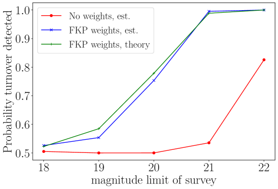
Figure 9: The probability that a turnover has been measured as a function of the apparent magnitude limit of the survey. The case of no weights is indicated by the red solid points. The case of FKP weights is denoted by the blue crosses. The case where the mean measurement is replaced by the theoretical model, but again with FKP weighting, is given by the rotated green crosses.

To calculate the probability that a power spectrum turnover has been measured, we perform a likelihood ratio test. We do this for the above turnover model, as well as for the model where $\alpha=0$, which signifies the ‘no turnover’ case. For our adopted Gaussian likelihood models, this ratio can be written as:

$${\mathcal{R}}_{\rm rel}=\frac{L_{\rm no-turn}}{L_{\rm turn}}=\exp[-(\chi^{2}_{\rm no-turn}-\chi^{2}_{\rm turn})/2]\ ,$$ (7.3)

where $\chi^{2}_{\rm no-turn}$ and $\chi^{2}_{\rm turn}$ are the chi-square distributions:

$$\chi^{2}_{\rm no-turn} =\sum_{i}\frac{\left[P_{i}-P_{\rm no-turn}(k_{i})\right]^{2}}{\sigma^{2}_{i}}\ ;$$ (7.4)

$$\chi^{2}_{\rm turn} =\sum_{i}\frac{\left[P_{i}-P_{\rm turn}(k_{i})\right]^{2}}{\sigma^{2}_{i}}\ .$$ (7.5)

From this information we can now derive the probability that we have detected a turnover. From the constraint that $p_{\rm no-turn}+p_{\rm turn}=1$, and that the ratio of likelihoods is proportional to the probability ratios $L_{\rm no-turn}/L_{\rm turn}=p_{\rm no-turn}/p_{\rm turn}$, we have:

$$p_{\rm turn}=1-p_{\rm no-turn}=\frac{1}{1+{\mathcal{R}}_{\rm rel}}\ .$$ (7.6)

Thus, for each power spectrum measurement, we can calculate the $\chi^{2}$ value for both models, the relative probability, and then $p_{\rm turn}$.

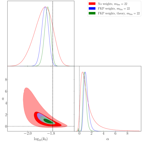
Figure 10: The 1-D and 2-D marginalised posterior distribution for the turnover scale $k_{0}$ and the large-scale slope $\alpha$, for the $m_{\rm lim}<22$, full-sky, mock galaxy catalogues. The red, blue and green lines in the top left and bottom right denote the full 1-D posterior distributions and the shaded contours in the bottom left panel denote the $68\%$ and $95\%$ confidence regions, for the case of, no weights, FKP weights and the theoretical predictions with FKP weights, respectively. The dashed line denotes the true peak of the linear power spectrum and the dotted line the case of no turnover.

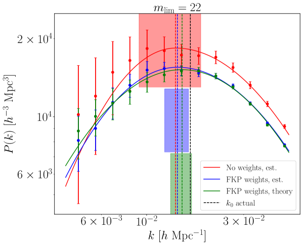
Figure 11: Power spectrum as a function of wavenumber for the deep, full-sky $m_{\rm lim}<22$ galaxy catalogue. The data points show show again the measurements from the 8 mocks, but where the red, blue and green colours denote the cases of no weighting, FKP weights and FKP weights, but with the measured signal swapped for our theoretical predictions, respectively. The solid lines show the results for the turnover model evaluated with the best-fit parameters. The dashed vertical lines give the the derived values of $k_{0}$ with shaded regions (with separate y ranges for clarity) showing the errors. The actual value of $k_{0}$ obtained from the linear theory spectrum is shown as the dashed vertical black line.

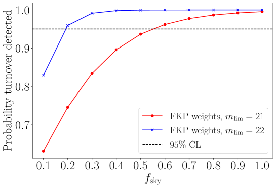
Figure 12: Detection probability of the turnover scale as a function of the sky fraction $f_{\rm sky}$ covered by our mock survey data. Red and blue points and lines show the results for the $m_{\rm lim}<21$ and $m_{\rm lim}<22$ catalogues. The dashed line indicates the 95% confidence limit threshold.

Figure 9 shows the turnover probability as a function of survey limiting magnitude, and for the three different cases listed above. We see that the ability to detect a turnover scale with 95% confidence in our magnitude limited catalogues is only achievable for our deepest two mocks ($m_{\rm lim}=21$ and $m_{\rm lim}=22$), and only when we employ the FKP weighting scheme. This result is independent of whether we use our actual measurements from the lightcones, or from the theoretical predictions. Conversely, in the absence of an optimal weighting scheme, we find that this simpler approach cannot unambiguously discern the turnover scale.

Figure 10 shows the joint 1-D and 2-D posterior distributions marginalised over all other parameters, for the $k_{0}$ and $\alpha$ from the MCMC analysis, and for the deep $m_{\rm lim}=22$ catalogue. These are the key parameters that determine whether the data has a turnover or not. We see that the joint constraints from all three scenarios considered find similar values for the turnover scale, with the FKP weighted data giving $k_{0}=0.0141\pm 0.0015\,h\,{\rm Mpc}^{-1}$. This value is within $1.5\sigma$ of the actual value for the turnover of the underlying linear power spectrum $k=0.0164\,h\,{\rm Mpc}^{-1}$ (represented in the plot as the vertical dashed black line). We also find that the joint constraints for the best-fit turnover slope parameter are, for the FKP weighted data, $\alpha=1.15^{0.25}_{-0.46}$. Thus the no turnover case corresponding to $\alpha=0$ can be convincingly rejected in our mock samples.

It is interesting to note that the slight bump in the measured power spectra at around $k\simeq 10^{-2}\,h\,{\rm Mpc}^{-1}$, which can be seen in Fig. 7, slightly flattens the top of the power spectrum. This has the effect of dragging the best fit turnover scale towards slightly larger scales and our range of values for $k_{0}$ lie slightly below the actual value of $k=0.0164\,h\,{\rm Mpc}^{-1}$. This analysis demonstrates some the difficulties in accurately measuring the turnover scale [for another recent look at this issue, in the context of HI surveys, see 81].

In Figure 11 we present again the measured power spectra for the $m_{\rm lim}<22$ catalogues, as a function of wavenumber. However, we now show the best-fit turnover models, overlay the best-fit values for the turnover scale $k_{0}$ for each data set and indicates the true turnover scale as measured from the input linear theory spectrum. One can see that while the models all fit the data very well, there is, as noted above, a small systematic underestimate of the true $k_{0}$. We partly attribute this to large-scale fluctuations in the estimated $P(k)$ points (see the red and blue points), which drags the fit to prefer smaller values of $k_{0}$. This is much less pronounced for the case where we use the lightcone theory predictions as $P(k)$ to determine $k_{0}$, however the underestimate remains.

7.3 Scaling to incomplete sky-coverage

Up to this point our analysis has focused on an all-sky survey, which is of most relevance to planned missions like SPHEREx [4]. However, we now attempt to relate our study to upcoming smaller, wide-angled, deep, galaxy redshift surveys. We do this by examining how the probability $p_{\rm turn}$ depends on surveyed sky fraction $f_{\rm sky}$. Recalling Eq. (5.8), we see that the error bars for our $P(k)$ estimates scale as $\sigma(k)\propto 1/\sqrt{N_{k}}$, where $N_{k}$ is the number of Fourier modes. This quantity scales as $N_{k}\propto{V^{\rm max}_{\mu}}$, i.e. the survey volume, which in turn is proportional to $f_{\rm sky}$. Thus we expect that $\sigma(k)\propto 1/\sqrt{f_{\rm sky}}$. Owing to the fact that we were only able to robustly detect the turnover scale for our deeper surveys, we will also restrict our attention to the $m_{\rm lim}=21$ and 22 catalogues. We now repeat the MCMC posterior estimation, but increasing the error bars by a factor of $1/\sqrt{f_{\rm sky}}$ for $f_{\rm sky}\in\{1.0,0.1\}$ in $0.1$ intervals.

Figure 12 shows the detection probability for the two deep catalogues as a function of the sky fraction $f_{\rm sky}$. We see that the $m_{\rm lim}<22$ catalogue is able to detect the turnover scale at a $\gtrsim 95\%$ confidence limit for sky fractions $\gtrsim 20\%$. For the shallower $m_{\rm lim}<21$ mock catalogue, we see that the sky fraction needs to be $\gtrsim 55\%$ for a similar level of detection.

Before moving on, it is important to note that here we have assumed that the shape of the power spectrum remains constant as the sky fraction is reduced. While this should hold true at smaller scales, depending on how the survey geometry changes, we may lose the ability to probe $k$-modes at the largest scales. This would decrease the number of data points past the turnover scale that we have available to constrain the model, and likely increase their errors. Furthermore, as discussed earlier in §5.4, the covariance matrix is non-diagonal due to the mask, and so true significance must be determined from a more advanced analysis and we leave this to future work.

8 Conclusions and discussion

Upcoming measurements of the large-scale structure of the Universe will probe ‘effective volumes’ that approach that of the entire observable Universe [4]. This will enable us to perform cosmological tests to an unprecedented precision. However, in order to extract the information from such data sets, we must ensure that we are also able to model the observable clustering signals with an unprecedented degree of both accuracy and precision. This work contributes to that effort. In this paper, we have performed a detailed study of the geometrical lightcone effect on the two-point galaxy clustering signal in Fourier space (the power spectrum) for a deep, flux-limited, full-sky survey.

In §2 we presented some key background concepts, in particular the observable density field on the past lightcone and the spherical-Fourier-Bessel expansion of the field.

In §3 we derived an expression for the galaxy two-point correlation function on the past-lightcone. We also presented the theory for the observable galaxy power spectrum, in real space, including the effects of shot-noise and luminosity dependent galaxy bias and for the case of an evolving luminosity function. We showed that the mean-redshift approximation biases the amplitude and shape of the galaxy power spectrum by more than $5\%$ for our cases considered, when compared to a model using the unequal time correlator.

In §4 we developed a series of approximations to the full analytic expressions that aided evaluation. We explored how the expressions would simplify for time separable models of the UETC. We derived approximations in the large-scale limit, finding that the observed power, unlike the linear theory, asymptoted to a constant value. On small scales, we were able to show that the observed spectrum reduced to a more tractable form. We also examined the fixed time approximation and showed that, provided that the time was carefully chosen, one could minimise the errors on this, but over a restricted range of wavenumbers and that nonlinear evolution would always break this approximation. Here we also discussed how to extend the model into the nonlinear regime.

In §5 we turned to validating our model, using $N$-body simulations. We did this by developing an algorithm to generate full-sky dark matter lightcones by using a quadratic interpolation scheme to interpolate the world lines of all particles in a piecewise fashion between consecutive snapshots. We then used this as the base from which we generated out mock galaxy samples. We also developed a parallel code for estimating the power spectrum from large data sets, making use of an interlacing technique to obtain accurate results all the way up to the Nyquist frequency. We then compared these measured spectra against our theoretical predictions in §6 and found excellent agreement on the scales considered. However, some small discrepancies were found on small scales, which we attributed to the breakdown of the specific form of our nonlinear corrections.

In §7 we revisited the question of detecting the turnover scale of the power spectrum as a probe for the epoch of matter-radiation equality in the early universe. Following the method outlined in [49] and [80] we used our mock catalogues for various flux-limited surveys to measured a peak scale $k_{0}$ and the power-law slope $\alpha$ of the spectrum red-wards of the peak. We did this by performing a standard Bayesian parameter estimation scheme, where we explored the full parameter space using an efficient MCMC sampler. We found that only galaxy catalogues with $m_{\rm lim}\gtrsim 21$, in conjunction with FKP weighting scheme, had sufficient statistical power to detect the turnover with a probability $P\gtrsim 95\%$. By rescaling the covariance by the inverse of the sky-fraction, $1/f_{\rm sky}$, we recomputed the posterior distributions and found that the detection level was maintained for surveys with $m_{\rm lim}=21$ and $m_{\rm lim}=22$ for sky coverages greater than $50\%$ and $20\%$, respectively.

There are several possible directions in which this work can be extended. First, the model that we have developed is overly simplistic, in that we worked only in real space. In reality, the radial positions are affected by redshift space distortions. In this work we have only considered the expression for the real space power spectrum monopole. Extending the derivations from section §3 will also be important. This will also go hand-in-hand with development for the power-spectrum multipoles [for recent developments along these lines see 45, 46, 83, 84, 85]. However, in the end, these extensions are unlikely to change our conclusions concerning the turnover scale, since it is expected that for such large scales these distortions would only modify the amplitude of the signal and not the shape of the peak or its signal-to-noise. Second, we restricted our attention to full-sky surveys only. One should take account of the angular mask. Third, although we included a linear luminosity dependent bias and a generic time separable model for the UETC, more realistic treatment of galaxy bias is needed. We were unable to explore this with our simulations, due to resolution issues and the difficulty in interpolating halo positions between snapshots [although see 65, for an example of how this could be done.].

All three of these extensions make the model in Eq. (4.5) more complicated, and thus it also becomes necessary to improve the numerical methods used to forward model the theory. Our current method employs a set of adaptive numerical quadrature routines to compute the full Bessel function integrals on large scales. This brute force approach is somewhat slow and prone to convergence issues. A more efficient way of such integrals would be through the FFTLog algorithm of [86]. Another interesting prospect of being able to measure the power spectrum accurately on large scales, particularly past the turnover scale, is the increased ability to constrain signatures of primordial non-Gaussianity. Such measurements remain one of the most promising probes to discriminate between inflationary models, with the most stringent constraints currently coming from measurements of the CMB [87]. However, as we probe out to larger volumes with late-time Universe surveys, measurements of the large-scale structures will be highly complimentary and competitive [4, 88, 89].

Appendix A Spherical-Fourier-Bessel expansion

In this appendix we provide a short overview of the Spherical-Fourier-Bessel (hereafter SFB) expansion of the overdensity field. To begin, consider the overdensity field $\Delta(\eta,{\bf r})$ written as a Fourier transform over our flat-space geometry:

$$\Delta(\eta,{\bf r})=\int\frac{{\rm d}^{3}{\bf k}}{(2\pi)^{3}}\Delta(\eta,{\bf k})e^{-i{\bf k}\cdot{\bf r}}\ .$$ (A.1)

The plane wave can be expanded as a sum over spherical harmonics and spherical Bessel functions:

$$e^{i{\bf k}\cdot{\bf r}}=4\pi\sum_{\ell=0}^{\infty}\sum_{m=-\ell}^{\ell}i^{\ell}j_{\ell}(kr)Y_{\ell m}(\hat{{\bf k}})Y_{\ell m}^{*}(\hat{{\bf r}})\ .$$ (A.2)

On making use of this relation in Eq. (A.1) we find:

$$\Delta(\eta,{\bf r})=\sum_{\ell,m}(-i)^{\ell}Y_{\ell m}^{*}(\hat{{\bf r}})\int\frac{{\rm d}^{3}{\bf k}}{(2\pi)^{3}}4\pi j_{\ell}(kr)Y_{\ell m}(\hat{{\bf k}})\Delta(\eta,{\bf k})\ ,$$ (A.3)

where for simplicity we have compressed the double sum. Consider now the integral factor on the right-hand-side of the above expression, this can be split into a radial integral and a surface integral. The surface integral takes the form:

$$\int{\rm d}\hat{{\bf k}}\ Y_{\ell m}(\hat{{\bf k}})\Delta(\eta,{\bf k})=(-1)^{\ell}\Delta_{\ell m}^{*}(\eta,k)\ ,$$ (A.4)

where

$$\Delta_{\ell m}(\eta,k)=\int{\rm d}\hat{{\bf k}}\ Y_{\ell m}^{*}(\hat{{\bf k}})\Delta(\eta,{\bf k}).$$ (A.5)

On substituting this all back into Eq. (A.3) gives:

$$\Delta(\eta,{\bf r}) = \sum_{\ell,m}^{\ell}Y_{\ell m}^{*}(\hat{{\bf r}})\Delta_{\ell m}^{*}(\eta,r)=\sum_{\ell,m}Y_{\ell m}(\hat{{\bf r}})\Delta_{\ell m}(\eta,r)\ ,$$ (A.6)

where the second equality follows from the reality of the density field, i.e. $\Delta(\eta,{\bf r})=\Delta^{*}(\eta,{\bf r})$ and where in the above we have defined the amplitudes of the spherical harmonics as:

$$\Delta_{\ell m}(\eta,r) \equiv (-i)^{\ell}\int\frac{{\rm d}^{3}{\bf k}}{(2\pi)^{3}}j_{\ell}(kr)\Delta_{\ell m}(\eta,k)\ .$$ (A.7)

In this work we will make extensive use of these relations.

Appendix B Power spectrum on the past light-cone

B.1 A fiducial galaxy redshift survey

Let us define our fiducial galaxy survey: suppose that we have observed $N^{\rm tot}_{\rm g}$ galaxies and to the $i$th galaxy we assign a luminosity $L_{i}$, redshift $z_{i}$ and angular position on the sky $\bm{\Omega}_{i}=\bm{\Omega}(\theta_{i},\phi_{i})$. If we specify the background FLRW spacetime, then we may convert the redshift into a comoving radial geodesic distance $\chi_{i}=\chi(z_{i})$. A galaxy’s comoving position vector on the past lightcone may now be expressed as ${\bf r}_{i}={\bf r}(\chi_{i},\bm{\Omega}_{i})$ (c.f. Eq. (2.2)).

The survey mask function depends on both the position and luminosity of galaxies, given an adopted flux limit $m_{\rm lim}$. In this work we shall take the angular and radial parts of the survey mask function to be separable:

$$\Theta({\bf r}|L)=\Theta(\bm{\Omega})\Theta(\chi|L)\ .$$ (B.1)

The angular part of the mask may be written most simply as:

$$\Theta(\bm{\Omega})=\left\{\begin{array}[]{cc}1\ ;&[{\bm{\Omega}}\in\{{\bm{\Omega}}_{\mu}\}]\\ 0\ ;&[\rm otherwise]\end{array}\ ,\right.$$ (B.2)

where $\{\bm{\Omega}_{\mu}\}$ is the set of angular positions that lie inside the survey area. In this work we shall for simplicity assume that we are dealing with a full-sky survey and so will neglect the angular mask. The radial mask function may be written:

$$\Theta(\chi|L)=\left\{\begin{array}[]{cc}1\ ;&[{\chi}\leq\chi_{\rm max}(L)]\\ 0\ ;&[\rm otherwise]\end{array}\ ,\right.$$ (B.3)

where $\chi_{\rm max}(L)$ is the maximum distance out to which a galaxy of luminosity $L$ could have been detected.

The survey volume for galaxies with luminosity $L$ is simply the integral of the mask function over all space:

$${V^{\rm max}_{\mu}}(L)=\int\Theta({\bf r}|L)dV,$$ (B.4)

where $dV$ is the comoving volume element at position vector ${\bf r}$ (for a flat universe $dV=d^{3}r=\chi^{2}d\Omega d\chi$) . In what follows it will be also useful to note that the relation $\chi_{\rm max}(L)$ may be inverted to obtain the minimum galaxy luminosity that could have been detected at radial position $\chi(z)$ in the survey. We shall write this as:

$$\left[{L_{\rm min}}({\bf r})/h^{-2}L_{\odot}\right]=10^{-\frac{2}{5}\left(m_{\rm lim}-25-M_{\odot}\right)}\left[d_{\rm L}({\bf r})/\,h^{-1}{\rm Mpc}\right]^{2}\ ,$$ (B.5)

where $m_{\rm lim}$ is the apparent magnitude limit of the survey, $M_{\odot}$ is the absolute magnitude of the sun, $h$ is the dimensionless Hubble parameter and $d_{\rm L}$ is the luminosity distance (for a flat universe $d_{\rm L}(z)=(1+z)\chi(z)$). Thus for any general function ${\mathcal{B}(\chi,L)}$, we have the useful integral relations:

$$\int_{0}^{\infty}dL\int_{0}^{\infty}d\chi\Theta(\chi|L)\mathcal{B}(\chi,L) =\int_{0}^{\infty}dL\int_{0}^{\chi_{\rm max}(L)}d\chi\mathcal{B}(\chi,L)$$ (B.6)

$$=\int_{0}^{\infty}d\chi\int_{{L_{\rm min}}(\chi)}^{\infty}dL\mathcal{B}(\chi,L)\ .$$

B.2 Galaxy density field on the lightcone as a Dirac delta function expansion

In general the spatial density distribution of galaxies, per unit luminosity, at position ${\bf x}(\chi,\bm{\Omega})$ on the lightcone may be written as a sum over Dirac delta functions:

$$n^{\rm LC}_{{\rm g}}({\bf r},L)=\sum_{i=1}^{N}\delta^{\rm D}(L-L_{i})\delta^{\rm D}({\bf r}-{\bf r}_{i})\ .$$ (B.7)

Let us define the galaxy field ${\mathcal{F}}$, which is related to the over-density of galaxies. This can be written:

$$F^{\rm LC}({\bf r}) =A\left[n^{\rm LC}({\bf r})-\alpha\,n^{\rm LC}_{\rm s}({\bf r})\right]$$

$$=A\int dLw({\bf r},L)\Theta({\bf r}|L)\left[n_{{\rm g}}^{\rm LC}({\bf r},L)-\alpha n_{s}^{\rm LC}({\bf r},L)\right]\ ,$$ (B.8)

where $w({\bf r},L)$ is a weight function that may depend on a galaxies position in the survey and also its luminosity. $n^{\rm LC}_{s}({\bf r},L)$ represents the number density of galaxies in a mock sample that has no intrinsic spatial correlations, and whose density is $1/\alpha$ times that of the true galaxy field at that mass. Note that whilst the field $n^{\rm LC}_{s}({\bf r},L)$ has no intrinsic spatial correlations it does obey a luminosity function, which is closely related to the galaxy luminosity function of $\left<n^{\rm LC}_{{\rm g}}({\bf r},L)\right>$. The choice for the normalisation parameter $A$ will be given later.

B.3 Statistical properties of the past-lightcone galaxy density field

We desire to be able to perform various statistical analyses of the field $F^{\rm LC}$. To understand how we should do this, let us compute its ensemble average value. This can be written,

$$\left<F^{\rm LC}({\bf r})\right> =A\left[\left<n_{{\rm g}}^{\rm LC}({\bf r})\right>-\alpha\,\left<n_{\rm s}^{\rm LC}({\bf r})\right>\right]$$

$$=A\int dLw({\bf r},L)\Theta({\bf r}|L)\left[\left<n_{{\rm g}}^{\rm LC}(\eta^{\prime},{\bf r},L)\right>-\alpha\left<n_{s}^{\rm LC}(\eta^{\prime},{\bf r},L)\right>\right]\ ,$$ (B.9)

where the angled brackets denote an ensemble average in the following sense:

$$\left<B(\left\{{\bf r}_{i},L_{i}\right\}|\eta)\right>\equiv\int{\rm d}^{3}{\bf r}_{1}\dots\rm d^{3}{\bf r}_{N}dL_{1}\dots dL_{N}p^{\rm LC}({\bf r}_{1},\dots,{\bf r}_{N},L_{1},\dots,L_{N}|\eta)B(\left\{{\bf r}_{i}(\eta),L_{i}(\eta)\right\})\ .$$ (B.10)

In the above $p^{\rm LC}({\bf r}_{1},\dots,{\bf r}_{N},L_{1},\dots,L_{N})$ is the $N$-point joint probability distribution for the $N$ galaxies being located at the set of spatial positions $\{{\bf r}_{i}\}$ on the lightcone and having the set of luminosities $\{L_{i}\}$. Thus, the first expectation on the right-hand side of Eq. (B.9) can be written as:

$$\left<n_{{\rm g}}^{\rm LC}({\bf r},L)\right> =\int\prod_{l=1}^{N}\left\{{\rm d}^{3}{\bf r}_{l}dL_{l}\right\}p^{\rm LC}({\bf r}_{1},\dots,{\bf r}_{N},L_{1},\dots,L_{N})\sum_{i=1}^{N}\delta^{\rm D}({\bf r}-{\bf r}_{i})\delta^{\rm D}(L-L_{i})$$

$$=\sum_{i=1}^{N}p^{\rm LC}({\bf r},L)=Np^{\rm LC}({\bf r},L)\ .$$ (B.11)

On the first line we inserted the expansion of the galaxy density field from Eq. (B.7) and to obtain the second we integrated over the sum of Dirac delta functions. The quantity $p^{\rm LC}({\bf r},L)$ can be simplified in the following way:

$$p^{\rm LC}({\bf r},L)=p^{\rm LC}({\bf r})p^{\rm LC}(L|{\bf r})=\frac{1}{{V_{\mu}}}\frac{\phi(L|{\bf r})}{N/{V_{\mu}}}=\frac{\phi(L|{\bf r})}{N}\ ,$$ (B.12)

where the first equality uses Bayes theorem, the second equality assumes that galaxies can be found anywhere inside the survey volume – note that this is irrespective of whether or not the galaxy would be observable. In the above $\phi(L|{\bf r})$ is the galaxy luminosity function (hereafter GLF), which gives us the number density of galaxies per unit luminosity, where the dependence on ${\bf r}$ indicates that GLF may evolve with redshift. Thus, as desired, we conclude that

$$\left<n^{\rm LC}_{{\rm g}}({\bf r},L)\right>=\phi(L|{\bf r})\ .$$ (B.13)

Turning to the second expectation value, we note that the only difference between $\left<n^{\rm LC}_{{\rm g}}({\bf r},L)\right>$ and $\left<n^{\rm LC}_{s}({\bf r},L)\right>$ is the artificially increased space density of galaxies and the absence of any intrinsic clustering. Hence, we likewise conclude that $\alpha\left<n^{\rm LC}_{s}({\bf r},L)\right>=\phi(L|{\bf r})$. Putting this all together, we arrive at the result that $F^{\rm LC}$ is a mean-zero field:

$$\left<F^{\rm LC}({\bf r})\right>=0\ .$$ (B.14)

B.4 An estimator for the galaxy power spectrum on the past lightcone

The correlation of the Fourier modes of the observed lightcone galaxy field $F^{\rm LC}$ can be written:

$$\left<F^{\rm LC}({\bf q}_{1})F^{\rm LC}({\bf q}_{2})\right> =\prod_{l=1}^{2}\left\{A\int{\rm d}^{3}{\bf r}_{l}{\rm e}^{i{\bf q}_{l}\cdot{\bf r}_{l}}\right\}\left<\left[n^{\rm LC}_{{\rm g}}({\bf r}_{1})-\alpha\,n^{\rm LC}_{\rm s}({\bf r}_{1})\right]\left[n^{\rm LC}_{{\rm g}}({\bf r}_{2})-\alpha\,n^{\rm LC}_{\rm s}({\bf r}_{2})\right]\right>$$

$$=\prod_{l=1}^{2}\left\{A\int{\rm d}^{3}{\bf r}_{l}{\rm e}^{i{\bf q}_{l}\cdot{\bf r}_{l}}\int dL_{1}w({\bf r}_{l},L_{l})\Theta({\bf r}_{l}|L_{l})\right\}\Big{[}\left<n^{\rm LC}_{{\rm g}}({\bf r}_{1},L_{1})n^{\rm LC}_{{\rm g}}({\bf r}_{2},L_{2})\right>$$

$$-2\alpha\left<n^{\rm LC}_{{\rm g}}({\bf r}_{1},L_{1})n^{\rm LC}_{\rm s}({\bf r}_{2},L_{2})\right>+\alpha^{2}\left<n^{\rm LC}_{\rm s}({\bf r}_{1},L_{1})n^{\rm LC}_{\rm s}({\bf r}_{2},L_{2})\right>\Big{]}\ ,$$ (B.15)

where in obtaining the second line we made use of Eq. (B.8) and assumed that $\left<n^{\rm LC}_{\rm s}({\bf r}_{1},L_{1})n^{\rm LC}_{{\rm g}}({\bf r}_{2},L_{2})\right>=\left<n^{\rm LC}_{\rm g}({\bf r}_{1},L_{1})n^{\rm LC}_{\rm s}({\bf r}_{2},L_{2})\right>$. To proceed further we need to compute the expectations $\left<n^{\rm LC}_{{\rm g}}({\bf r}_{1},L_{1})n^{\rm LC}_{{\rm g}}({\bf r}_{2},L_{2})\right>$ and to simplify the notation we shall use the shorthand notation $\langle n_{\rm g}n^{\prime}_{\rm g}\rangle_{\rm LC}\equiv\langle n^{\rm LC}_{\rm g}({\bf r},L)n^{\rm LC}_{\rm g}({\bf r}^{\prime},L^{\prime})\rangle$, and similarly for $\langle n_{\rm g}n^{\prime}_{s}\rangle_{\rm LC},\,\langle n_{s}n^{\prime}_{s}\rangle_{\rm LC}$. On inserting the delta function expansion of Eq. (B.7) we get:

$$\left<n_{\rm g}n^{\prime}_{\rm g}\right>_{\rm LC}=\int\prod_{l=1}^{N}\left\{{\rm d}^{3}{\bf r}_{l}dL_{l}\right\}p^{\rm LC}({\bf r}_{1},\dots,{\bf r}_{N},L_{1},\dots,L_{N})\sum_{i,j}^{N}\delta^{\rm D}({\bf r}-{\bf r}_{i})\delta^{\rm D}(L-L_{i})\delta^{\rm D}({\bf r}^{\prime}-{\bf r}_{j})\delta^{\rm D}(L^{\prime}-L_{j})\ .$$

The double sum can be broken up into the terms where $(i\neq j)$ and the terms where $(i=j)$, whereupon

$$\left<n_{\rm g}n^{\prime}_{\rm g}\right>_{\rm LC} =\int\prod_{l=1}^{N}\left\{{\rm d}^{3}{\bf r}_{l}dL_{l}\right\}p^{\rm LC}({\bf r}_{1},\dots,{\bf r}_{N},L_{1},\dots,L_{N})\left[\sum_{i\neq j}^{N}\delta^{\rm D}({\bf r}-{\bf r}_{i})\delta^{\rm D}(L-L_{i})\delta^{\rm D}({\bf r}^{\prime}-{\bf r}_{j})\delta^{\rm D}(L^{\prime}-L_{j})\right.$$

$$\hskip 85.35826pt+\left.\sum_{i=j}^{N}\delta^{\rm D}({\bf r}-{\bf r}_{i})\delta^{\rm D}({\bf r}^{\prime}-{\bf r}_{i})\delta^{\rm D}(L-L_{i})\delta^{\rm D}(L^{\prime}-L_{i})\right]$$

$$=\sum_{i\neq j}^{N}p^{\rm LC}({\bf r},{\bf r}^{\prime},L,L^{\prime})+\sum_{i=j}^{N}p^{\rm LC}({\bf r},L)\delta^{\rm D}({\bf r}-{\bf r}^{\prime})\delta^{\rm D}(L-L^{\prime})$$

$$=N(N-1)p^{\rm LC}({\bf r},{\bf r}^{\prime},L,L^{\prime})+Np^{\rm LC}({\bf r},L)\delta^{\rm D}({\bf r}-{\bf r}^{\prime})\delta^{\rm D}(L-L^{\prime})\ .$$ (B.16)

In order to proceed further, we need to specify the joint probability density distribution for obtaining galaxies at positions ${\bf r}$ and ${\bf r}^{\prime}$ and with masses $L$ and $L^{\prime}$. This we do through the introduction of correlation functions:

$$p^{\rm LC}({\bf r},{\bf r}^{\prime},L,L^{\prime}) \equiv p^{\rm LC}({\bf r},L)p^{\rm LC}({\bf r}^{\prime},L^{\prime})\left[1+\left<\Delta^{\rm LC}({\bf r}_{1}|L_{1})\Delta^{\rm LC}({\bf r}_{2}|L_{2})\right>\right]$$

$$=\frac{1}{N^{2}}\phi(L|{\bf r})\phi(L^{\prime}|{\bf r}^{\prime})\left[1+\left<\Delta^{\rm LC}({\bf r}_{1}|L_{1})\Delta^{\rm LC}({\bf r}_{2}|L_{2})\right>\right]\ ,$$ (B.17)

where $\left<\Delta^{\rm LC}({\bf r}_{1}|L_{1})\Delta^{\rm LC}({\bf r}_{2}|L_{2})\right>$ is the two-point cross-correlation function of galaxies with luminosities $L$ and $L^{\prime}$ at positions ${\bf r}$ and ${\bf r}^{\prime}$ on the past lightcone. On use of the above definition in Eq. (B.16), we find

$$\left<n_{\rm g}n^{\prime}_{\rm g}\right>_{\rm LC}\approx\frac{}{}\phi(L|{\bf r})\phi(L^{\prime}|{\bf r}^{\prime})\left[1+\left<\Delta^{\rm LC}({\bf r}|L)\Delta^{\rm LC}({\bf r}^{\prime}|L^{\prime})\right>\right]+\phi(L|{\bf r})\delta^{\rm D}({\bf r}-{\bf r}^{\prime})\delta^{\rm D}(L-L^{\prime})\ ,$$ (B.18)

where in arriving at the last equality we have assumed that $N\gg 1$ and therefore $N-1\approx N$. We may now write down directly the remaining expectation values that enter Eq. (B.15):

$$\left<n_{\rm g}n^{\prime}_{s}\right>_{\rm LC} = \alpha^{-1}\phi(L|{\bf r})\phi(L^{\prime}|{\bf r}^{\prime})\ ;$$

$$\langle n_{s}n^{\prime}_{s}\rangle_{\rm LC} = \alpha^{-2}\phi(L|{\bf r})\phi(L^{\prime}|{\bf r}^{\prime})+\alpha^{-1}\phi(L|{\bf r})\delta^{\rm D}({\bf r}-{\bf r}^{\prime})\delta^{\rm D}(L-L^{\prime})\ .$$ (B.19)

On inserting these into Eq. (B.15) we find:

$$\left<F^{\rm LC}({\bf q}_{1})F^{\rm LC}({\bf q}_{2})\right> =\prod_{l=1}^{2}\left\{A\int{\rm d}^{3}{\bf r}_{l}{\rm e}^{i{\bf q}_{l}\cdot{\bf r}_{l}}\int dL_{l}w({\bf r}_{l},L_{l})\Theta({\bf r}_{l}|L_{l})\right\}\Big{[}\phi(L_{1}|{\bf r}_{1})\phi(L_{2}|{\bf r}_{2})$$

$$\times\left<\Delta^{\rm LC}({\bf r}_{1}|L_{1})\Delta^{\rm LC}({\bf r}_{2}|L_{2})\right>+\phi(L_{1}|{\bf r}_{1})\delta^{\rm D}({\bf r}_{1}-{\bf r}_{2})\delta^{\rm D}(L_{1}-L_{2})\Big{]}\ .$$ (B.20)

Let us now focus on the first term in square brackets on the right-hand-side of Eq. (B.20), and let us assume that the luminosity dependence of the lightcone correlation function scales in the following way:

$$\left<\Delta^{\rm LC}({\bf r}_{1}|L_{1})\Delta^{\rm LC}({\bf r}_{2}|L_{2})\right>=b(L_{1}|\chi_{1})b(L_{2}|\chi_{2})\left<\Delta^{\rm LC}({\bf r}_{1})\Delta^{\rm LC}({\bf r}_{2})\right>\ .$$ (B.21)

Under this assumption, the Fourier mode correlation takes the form: [31]:

$$\left<F^{\rm LC}({\bf q}_{1})F^{\rm LC}({\bf q}_{2})\right> =\prod_{l=1}^{2}\left\{A\int{\rm d}^{3}{\bf r}_{l}{\rm e}^{i{\bf q}_{l}\cdot{\bf r}_{l}}n^{\rm LC}_{\rm Eff}({\bf r}_{l})b^{\rm LC}_{\rm Eff}({\bf r}_{l})\right\}\left<\Delta^{\rm LC}({\bf r}_{1})\Delta^{\rm LC}({\bf r}_{2})\right>$$ (B.22)

where the correlator $\left<\Delta({\bf r}_{1})\Delta({\bf r}_{2})\right>$ is that of the matter on the past lightcone, as given in Eq. (3.10) and where we have defined the effective galaxy bias and number density as:

$$b^{\rm LC}_{\rm Eff}(\chi) \equiv\frac{\int^{\infty}_{{L_{\rm min}}(\chi)}dLw({\bf r},L)\phi(L|{\bf r})b(L|\chi)}{\int^{\infty}_{{L_{\rm min}}(\chi)}dLw({\bf r},L)\phi(L|{\bf r})}\ ;$$ (B.23)

$$n^{\rm LC}_{\rm Eff}(\chi) \equiv\int^{\infty}_{{L_{\rm min}}(\chi)}dLw({\bf r},L)\phi(L|{\bf r}).$$ (B.24)

Note, in the case of no luminosity dependent biasing of clustering, such that $b(L|\chi)=1$, then $b^{\rm LC}_{\rm Eff}(\chi)=1$ and $n^{\rm LC}_{\rm Eff}(\chi)=w({\bf r})n^{\rm LC}_{0}(\chi)$.

Let us now inspect the second term in square brackets in Eq. (B.20). On integrating over ${\bf r}_{2}$ and $L_{2}$, and setting ${\bf q}_{2}=-{\bf q}_{1}$ this gives the shot-noise contribution [31]:

$$P^{\rm LC}_{\rm shot} =A^{2}\int{\rm d}^{3}{\bf r}\int dLw^{2}({\bf r},L)\Theta({\bf r}|L)\phi(L|{\bf r})$$

$$=4\pi A^{2}\int_{0}^{\infty}d\chi\chi^{2}\int_{{L_{\rm min}}(\chi)}^{\infty}dLw^{2}(\chi,L)\phi(L|\chi)$$ (B.25)

where in obtaining the above result we have made use of the fact that $\Theta^{2}({\bf r}|L)=\Theta({\bf r}|L)$ and we have set $|{\bf r}|=\chi$. If the weight function is assumed to be independent of galaxy luminosity, then the shot-noise term reduces to the standard expression from FKP:

$$P^{\rm LC}_{\rm shot} \xLongrightarrow[w({\bf r}|L)=w({\bf r})]{}4\pi A^{2}\int_{0}^{\infty}d\chi\chi^{2}w^{2}(\chi)n^{\rm LC}_{0}(\chi)$$ (B.26)

where the mean number density of galaxies on the past lightcone is given by:

$$n^{\rm LC}_{0}(\chi)\equiv\int_{{L_{\rm min}}(\chi)}^{\infty}dL\phi(L|\chi)\ .$$ (B.27)

Appendix C Modelling the evolving luminosity function and mock generation

C.1 The evolving luminosity function

In this section, we detail how the galaxy number density on the lightcone, $n_{0}^{\rm{LC}}(r)$, is calculated. To do this, we use the following formula:

$$n_{0}^{\rm{LC}}(r)=\int^{M_{\rm{lim}}(r)-5\log_{10}h}_{-\infty}\phi(M,r)dM\ .$$ (C.1)

In the above expression $\phi(M,r)$ is the evolving Schechter luminosity function, and in terms of absolute magnitudes this has the form:

$$\phi(M,r) = \frac{2}{5}\phi^{*}(r)\ln(10)10^{\frac{2}{5}(\alpha+1)[M^{*}(r)-M]}\exp\big{(}-10^{\frac{2}{5}[M^{*}(r)-M]}\big{)}\ .$$ (C.2)

When modelling the evolution, we follow [66] and let the two parameters $M^{*}(r)$ and $\phi^{*}(r)$ evolve with comoving radial distance, but keep the faint-end slope $\alpha$ fixed. For the evolving parameters we use the functional forms given in [66]:

$$M^{*}(z) = M^{*}(z_{0})-Q(z-z_{0})\ ;$$ (C.3)

$$\phi^{*}(z) = \phi^{*}(0)10^{0.4Pz}\ .$$ (C.4)

We take the 5 free parameters to be those obtained from fitting the $r$-band measurements for the combination of blue and red galaxies in the phase 1 GAMA data. Values are: $P=1.6$, $Q=0.2$, $\alpha=-1.23$, $M^{*}-5\log h=-20.7$ and $\phi^{*}=0.94\times 10^{-2}h^{3}\mathrm{Mpc}^{-3}$. We set the fiducial redshift to $z_{0}=0.1$, which is the redshift to which the magnitudes were $K$-corrected.

The lower limit on the integral in Eq. (C.1) is the largest possible absolute magnitude that is detectable, given the apparent magnitude limit $m_{\rm lim}$, at a given comoving radial distance $r$. This has the form:

$$M_{\rm{lim}}(r)-5\log_{10}h =m_{\rm{lim}}-5\log_{10}\left(\frac{d_{\rm L}(r)}{1\,h^{-1}{\rm Mpc}}\right)-25\ .$$ (C.5)

We use Eq. (C.1) in various stages of this work: first, in our theoretical modelling of the window-convolved power spectrum on the lightcone Eq. (3.18). Second, we use it for sampling magnitudes for our lightcone $N$-body simulations, so as to make magnitude-cut catalogues to mimic galaxy samples that would be observed by a real survey.

C.2 Sampling luminosities from the evolving Schechter Function

The method that we employ to sample luminosities from a prescribed galaxy luminosity function can be described as follows. First, we draw samples from a uniform random distribution $u(R)$, where $R\in[0,1]$. Second, these samples can be translated into random luminosities $L$, by following the probability integral transform method discussed in [91]. The steps for this can be summarised: from the transformation of random variables we have

$$|u(R)dR|=|p(L|r)dL|,$$ (C.6)

where $u(R)=1$ and $p(L)=\phi(L|r)/\bar{n(r)}$, with $\phi(L|r)$ being the desired GLF and $\bar{n}(r)$ the mean number density of the survey at comoving radial distance $r$. On integrating both sides of the above equation we find:

$$R=\int_{0}^{R}u(R^{\prime})dR^{\prime}=\int_{L_{\rm min}(r)}^{L}p(L|r)dL=\Phi(L|r)\ .$$ (C.7)

Provided that we can invert the cumulative distribution function $\Phi$, we can sample luminosities through the relation:

$$L=\Phi^{-1}(R)\ .$$ (C.8)

This recipe will allow us to generate a set of luminosities whose distribution follows the form specified by $p(L|r)$. In some cases the inversion of $\Phi$ can be done analytically. However, for more complex functions this can most efficiently be achieved thorough the use of a cubic spline function to build the inverse.

In this work, we want to sample from the evolving Schechter function (discussed in the previous section) with luminosities in the range $L\in[L_{\rm{min}},L_{\rm{max}}]$ and for numerical ease we choose $L_{\rm{max}}=100L^{*}$. The minimum luminosity $L_{\rm{min}}(r)$ is determined from the apparent magnitude cut and the comoving distance $r$ at which we are observing the galaxies (c.f. Eq. (B.5)). For the Schechter function GLF we can identify the function $p(L|r)$ as (suppressing the $r$ dependence for simplicity):

$$p(L|r) =\frac{x^{\alpha}{\rm e}^{-x}(L^{*})^{-1}}{\int_{L_{\rm{min}}}^{L_{\rm{max}}}x^{\alpha}{\rm e}^{-x}dx}\ \ \ ;\ \ \ x\equiv L/L^{*}\ .$$ (C.9)

Making use of the incomplete gamma function notation, we see that the cumulative distribution function can then be written:

$$\Phi(L)=\int_{L_{\rm min}}^{L}p(L|)dL =\frac{\int_{L_{\rm min}}^{L}dxx^{\alpha}{\rm e}^{-x}}{\int_{L_{\rm min}}^{L_{\rm max}}dxx^{\alpha}{\rm e}^{-x}}$$

$$=\frac{\Gamma(\alpha+1,L/L^{*})-\Gamma(\alpha+1,L_{\rm max}/L^{*})}{\Gamma(\alpha+1,L_{\rm min}/L^{*})-\Gamma(\alpha+1,L_{\rm max}/L^{*})}\ .$$ (C.10)

We repeat this sampling for a range of redshift values, covering the minimum and maximum redshift of our survey, and create a larger 2-d spline of the overall relationship.

References

- [1] DESI Collaboration, A. Aghamousa, J. Aguilar, S. Ahlen, S. Alam, L.E. Allen et al., The DESI Experiment Part I: Science,Targeting, and Survey Design, arXiv e-prints (2016) arXiv:1611.00036 [1611.00036].
- [2] J. Richard, J.P. Kneib, C. Blake, A. Raichoor, J. Comparat, T. Shanks et al., 4MOST Consortium Survey 8: Cosmology Redshift Survey (CRS), The Messenger 175 (2019) 50 [1903.02474].
- [3] R. Laureijs, J. Amiaux, S. Arduini, J.. Auguères, J. Brinchmann, R. Cole et al., Euclid Definition Study Report, ArXiv e-prints (2011) [1110.3193].
- [4] O. Doré, J. Bock, M. Ashby, P. Capak, A. Cooray, R. de Putter et al., Cosmology with the SPHEREX All-Sky Spectral Survey, arXiv e-prints (2014) arXiv:1412.4872 [1412.4872].
- [5] LSST, LSST Science Book, Version 2.0, ArXiv e-prints (2009) [0912.0201].
- [6] M. Tegmark, Measuring Cosmological Parameters with Galaxy Surveys, Physical Review Letters 79 (1997) 3806 [arXiv:astro-ph/9706198].
- [7] P.J.E. Peebles, The large-scale structure of the universe, Research supported by the National Science Foundation. Princeton, N.J., Princeton University Press, 1980. 435 p. (1980).
- [8] F. Bernardeau, S. Colombi, E. Gaztañaga and R. Scoccimarro, Large-scale structure of the Universe and cosmological perturbation theory, Phys. Rep. 367 (2002) 1 [arXiv:astro-ph/0112551].
- [9] Y.P. Jing, P. Zhang, W.P. Lin, L. Gao and V. Springel, The Influence of Baryons on the Clustering of Matter and Weak-Lensing Surveys, ApJL 640 (2006) L119 [astro-ph/0512426].
- [10] G. Somogyi and R.E. Smith, Cosmological perturbation theory for baryons and dark matter: One-loop corrections in the renormalized perturbation theory framework, PRD 81 (2010) 023524 [0910.5220].
- [11] I.G. McCarthy, S. Bird, J. Schaye, J. Harnois-Deraps, A.S. Font and L. van Waerbeke, The BAHAMAS project: the CMB-large-scale structure tension and the roles of massive neutrinos and galaxy formation, MNRAS 476 (2018) 2999 [1712.02411].
- [12] N. Kaiser, On the spatial correlations of Abell clusters, ApJL 284 (1984) L9.
- [13] J.N. Fry and E. Gaztanaga, Biasing and hierarchical statistics in large-scale structure, ApJ 413 (1993) 447 [arXiv:astro-ph/9302009].
- [14] P. Coles, Galaxy formation with a local bias, MNRAS 262 (1993) 1065.
- [15] A. Dekel and O. Lahav, Stochastic Nonlinear Galaxy Biasing, ApJ 520 (1999) 24 [arXiv:astro-ph/9806193].
- [16] T. Baldauf, U. Seljak, V. Desjacques and P. McDonald, Evidence for quadratic tidal tensor bias from the halo bispectrum, PRD 86 (2012) 083540 [1201.4827].
- [17] K.C. Chan, R. Scoccimarro and R.K. Sheth, Gravity and large-scale nonlocal bias, PRD 85 (2012) 083509 [1201.3614].
- [18] A. Eggemeier, R. Scoccimarro, R.E. Smith, M. Crocce, A. Pezzotta and A.G. Sánchez, Testing one-loop galaxy bias: Joint analysis of power spectrum and bispectrum, PRD 103 (2021) 123550 [2102.06902].
- [19] N. Kaiser, Clustering in real space and in redshift space, MNRAS 227 (1987) 1.
- [20] A.J.S. Hamilton, Linear Redshift Distortions: a Review, in The Evolving Universe, D. Hamilton, ed., vol. 231 of Astrophysics and Space Science Library, pp. 185–+, 1998.
- [21] R. Scoccimarro, Redshift-space distortions, pairwise velocities, and nonlinearities, PRD 70 (2004) 083007 [arXiv:astro-ph/0407214].
- [22] K. Yamamoto, H. Nishioka and Y. Suto, The Cosmological Light-Cone Effect on the Power Spectrum of Galaxies and Quasars in Wide-Field Redshift Surveys, ApJ 527 (1999) 488 [astro-ph/9908006].
- [23] T. Matsubara, The Correlation Function in Redshift Space: General Formula with Wide-Angle Effects and Cosmological Distortions, ApJ 535 (2000) 1 [astro-ph/9908056].
- [24] J. Yoo and U. Seljak, Wide-angle effects in future galaxy surveys, MNRAS 447 (2015) 1789 [1308.1093].
- [25] D. Bertacca, A. Raccanelli, N. Bartolo, M. Liguori, S. Matarrese and L. Verde, Relativistic wide-angle galaxy bispectrum on the light cone, PRD 97 (2018) 023531 [1705.09306].
- [26] C. Alcock and B. Paczynski, An evolution free test for non-zero cosmological constant, Nature 281 (1979) 358.
- [27] W.E. Ballinger, J.A. Peacock and A.F. Heavens, Measuring the cosmological constant with redshift surveys, MNRAS 282 (1996) 877 [astro-ph/9605017].
- [28] H.A. Feldman, N. Kaiser and J.A. Peacock, Power-spectrum analysis of three-dimensional redshift surveys, ApJ 426 (1994) 23 [arXiv:astro-ph/9304022].
- [29] M. Tegmark, How to measure CMB power spectra without losing information, PRD 55 (1997) 5895 [astro-ph/9611174].
- [30] K. Yamamoto, Optimal Weighting Scheme in Redshift-Space Power Spectrum Analysis and a Prospect for Measuring the Cosmic Equation of State, ApJ 595 (2003) 577 [astro-ph/0208139].
- [31] W.J. Percival, L. Verde and J.A. Peacock, Fourier analysis of luminosity-dependent galaxy clustering, MNRAS 347 (2004) 645 [arXiv:astro-ph/0306511].
- [32] R.E. Smith and L. Marian, Towards optimal estimation of the galaxy power spectrum, MNRAS 454 (2015) 1266 [1503.06830].
- [33] W.J. Percival, W. Sutherland, J.A. Peacock, C.M. Baugh, J. Bland-Hawthorn, T. Bridges et al., Parameter constraints for flat cosmologies from cosmic microwave background and 2dFGRS power spectra, MNRAS 337 (2002) 1068 [arXiv:astro-ph/0206256].
- [34] P.J.E. Peebles, Statistical Analysis of Catalogs of Extragalactic Objects. I. Theory, ApJ 185 (1973) 413.
- [35] C. Scharf, Y. Hoffman, O. Lahav and D. Lynden-Bell, Spherical harmonic analysis of IRAS galaxies : implications for the GreatAttractor and cold dark matter., MNRAS 256 (1992) 229.
- [36] C.A. Scharf and O. Lahav, Spherical Harmonic Analysis of the 2-JANSKY IRAS Galaxy Redshift Survey, MNRAS 264 (1993) 439.
- [37] K.B. Fisher, O. Lahav, Y. Hoffman, D. Lynden-Bell and S. Zaroubi, Wiener reconstruction of density, velocity and potential fields from all-sky galaxy redshift surveys, MNRAS 272 (1995) 885 [astro-ph/9406009].
- [38] A.F. Heavens and A.N. Taylor, A spherical harmonic analysis of redshift space, MNRAS 275 (1995) 483 [astro-ph/9409027].
- [39] H. Tadros, W.E. Ballinger, A.N. Taylor, A.F. Heavens, G. Efstathiou, W. Saunders et al., Spherical harmonic analysis of the PSCz galaxy catalogue: redshift distortions and the real-space power spectrum, MNRAS 305 (1999) 527 [astro-ph/9901351].
- [40] W.J. Percival, D. Burkey, A. Heavens, A. Taylor, S. Cole, J.A. Peacock et al., The 2dF Galaxy Redshift Survey: spherical harmonics analysis of fluctuations in the final catalogue, MNRAS 353 (2004) 1201 [arXiv:astro-ph/0406513].
- [41] A. Nicola, A. Refregier, A. Amara and A. Paranjape, Three-dimensional spherical analyses of cosmological spectroscopic surveys, PRD 90 (2014) 063515 [1405.3660].
- [42] F. Lanusse, A. Rassat and J.L. Starck, 3D galaxy clustering with future wide-field surveys: Advantages of a spherical Fourier-Bessel analysis, A&A 578 (2015) A10 [1406.5989].
- [43] M. Shiraishi, T. Okumura, N.S. Sugiyama and K. Akitsu, Minimum Variance Estimation of Galaxy Power Spectrum in Redshift Space, MNRAS (2020) [2005.03438].
- [44] E. Castorina and M. White, Beyond the plane-parallel approximation for redshift surveys, MNRAS 476 (2018) 4403 [1709.09730].
- [45] K. Yamamoto, M. Nakamichi, A. Kamino, B.A. Bassett and H. Nishioka, A Measurement of the Quadrupole Power Spectrum in the Clustering of the 2dF QSO Survey, Publications of the ASJ 58 (2006) 93 [astro-ph/0505115].
- [46] R. Scoccimarro, Fast estimators for redshift-space clustering, PRD 92 (2015) 083532 [1506.02729].
- [47] C. Blake and K. Glazebrook, Probing Dark Energy Using Baryonic Oscillations in the Galaxy Power Spectrum as a Cosmological Ruler, ApJ 594 (2003) 665 [astro-ph/0301632].
- [48] H.-J. Seo and D.J. Eisenstein, Probing Dark Energy with Baryonic Acoustic Oscillations from Future Large Galaxy Redshift Surveys, ApJ 598 (2003) 720 [arXiv:astro-ph/0307460].
- [49] C. Blake and S. Bridle, Cosmology with photometric redshift surveys, MNRAS 363 (2005) 1329 [astro-ph/0411713].
- [50] J. Binney and T. Quinn, Gaussian random fields in spherical coordinates, MNRAS 249 (1991) 678.
- [51] T.D. Kitching and A.F. Heavens, Unequal-time correlators for cosmology, PRD 95 (2017) 063522 [1612.00770].
- [52] K. Yamamoto, H. Nishioka and A. Taruya, The effect of bias and redshift distortions on a geometric test for the cosmological constant, arXiv e-prints (2000) astro [astro-ph/0012433].
- [53] M. Abramowitz and I.A. Stegun, Handbook of mathematical functions : with formulas, graphs, and mathematical tables, Dover (1970).
- [54] L. Clerkin, D. Kirk, O. Lahav, F.B. Abdalla and E. Gaztañaga, A prescription for galaxy biasing evolution as a nuisance parameter, MNRAS 448 (2015) 1389 [1405.5521].
- [55] J.L. Tinker, B.E. Robertson, A.V. Kravtsov, A. Klypin, M.S. Warren, G. Yepes et al., The Large-scale Bias of Dark Matter Halos: Numerical Calibration and Model Tests, ApJ 724 (2010) 878 [1001.3162].
- [56] J.E. McEwen, X. Fang, C.M. Hirata and J.A. Blazek, FAST-PT: a novel algorithm to calculate convolution integrals in cosmological perturbation theory, Journal of Cosmology and Astro-Particle Physics 2016 (2016) 015 [1603.04826].
- [57] R. Takahashi, M. Sato, T. Nishimichi, A. Taruya and M. Oguri, Revising the Halofit Model for the Nonlinear Matter Power Spectrum, ApJ 761 (2012) 152 [1208.2701].
- [58] R.E. Smith and R.E. Angulo, Precision modelling of the matter power spectrum in a Planck-like Universe, MNRAS 486 (2019) 1448 [1807.00040].
- [59] Planck Collaboration, P.A.R. Ade, N. Aghanim, C. Armitage-Caplan, M. Arnaud, M. Ashdown et al., Planck 2013 results. XVI. Cosmological parameters, A&A 571 (2014) A16 [1303.5076].
- [60] A. Lewis, A. Challinor and A. Lasenby, Efficient Computation of Cosmic Microwave Background Anisotropies in Closed Friedmann-Robertson-Walker Models, ApJ 538 (2000) 473 [astro-ph/9911177].
- [61] M. Crocce, S. Pueblas and R. Scoccimarro, Transients from initial conditions in cosmological simulations, MNRAS 373 (2006) 369 [arXiv:astro-ph/0606505].
- [62] V. Springel, The cosmological simulation code GADGET-2, MNRAS 364 (2005) 1105 [astro-ph/0505010].
- [63] R.E. Angulo, V. Springel, S.D.M. White, A. Jenkins, C.M. Baugh and C.S. Frenk, Scaling relations for galaxy clusters in the Millennium-XXL simulation, MNRAS 426 (2012) 2046 [1203.3216].
- [64] V. Springel, S.D.M. White, A. Jenkins, C.S. Frenk, N. Yoshida, L. Gao et al., Simulations of the formation, evolution and clustering of galaxies and quasars, Nature 435 (2005) 629 [astro-ph/0504097].
- [65] A.I. Merson, C.M. Baugh, J.C. Helly, V. Gonzalez-Perez, S. Cole, R. Bielby et al., Lightcone mock catalogues from semi-analytic models of galaxy formation - I. Construction and application to the BzK colour selection, MNRAS 429 (2013) 556 [1206.4049].
- [66] J. Loveday, P. Norberg, I.K. Baldry, S.P. Driver, A.M. Hopkins, J.A. Peacock et al., Galaxy and Mass Assembly (GAMA): ugriz galaxy luminosity functions, MNRAS 420 (2012) 1239 [1111.0166].
- [67] C. Blake, S. Brough, M. Colless, W. Couch, S. Croom, T. Davis et al., The WiggleZ Dark Energy Survey: the selection function and z = 0.6 galaxy power spectrum, MNRAS 406 (2010) 803 [1003.5721].
- [68] R.W. Hockney and J.W. Eastwood, Computer Simulation Using Particles, CRC Press (1981).
- [69] C.R. Harris, K.J. Millman, S.J. van der Walt, R. Gommers, P. Virtanen, D. Cournapeau et al., Array programming with NumPy, Nature 585 (2020) 357 [2006.10256].
- [70] P. Virtanen, R. Gommers, E. Burovski, T.E. Oliphant, D. Cournapeau, W. Weckesser et al., scipy/scipy: SciPy 1.2.1, Feb., 2019. 10.5281/zenodo.2560881.
- [71] Astropy Collaboration, T.P. Robitaille, E.J. Tollerud, P. Greenfield, M. Droettboom, E. Bray et al., Astropy: A community Python package for astronomy, A&A 558 (2013) A33 [1307.6212].
- [72] S.K. Lam, A. Pitrou and S. Seibert, Numba: A llvm-based python jit compiler, in Proceedings of the Second Workshop on the LLVM Compiler Infrastructure in HPC, LLVM ’15, (New York, NY, USA), Association for Computing Machinery, 2015, DOI.
- [73] L.D. Dalcin, R.R. Paz, P.A. Kler and A. Cosimo, Parallel distributed computing using Python, Advances in Water Resources 34 (2011) 1124.
- [74] H. Gomersall, Pyfftw, June, 2016. 10.5281/zenodo.59508.
- [75] Y.P. Jing, Correcting for the Alias Effect When Measuring the Power Spectrum Using a Fast Fourier Transform, ApJ 620 (2005) 559 [arXiv:astro-ph/0409240].
- [76] E. Sefusatti, M. Crocce, R. Scoccimarro and H.M.P. Couchman, Accurate estimators of correlation functions in Fourier space, MNRAS 460 (2016) 3624 [1512.07295].
- [77] V. Springel, R. Pakmor, O. Zier and M. Reinecke, Simulating cosmic structure formation with the GADGET-4 code, MNRAS 506 (2021) 2871 [2010.03567].
- [78] W. Sutherland, H. Tadros, G. Efstathiou, C.S. Frenk, O. Keeble, S. Maddox et al., The power spectrum of the Point Source Catalogue redshift survey, MNRAS 308 (1999) 289 [astro-ph/9901189].
- [79] S. Dodelson, Modern cosmology, Modern cosmology / Scott Dodelson. Amsterdam (Netherlands): Academic Press. ISBN 0-12-219141-2, 2003, XIII + 440 p. (2003).
- [80] G.B. Poole, C. Blake, D. Parkinson, S. Brough, M. Colless, C. Contreras et al., The WiggleZ Dark Energy Survey: probing the epoch of radiation domination using large-scale structure, MNRAS 429 (2013) 1902 [1211.5605].
- [81] S. Cunnington, Detecting the power spectrum turnover with H I intensity mapping, MNRAS 512 (2022) 2408 [2202.13828].
- [82] D. Foreman-Mackey, D.W. Hogg, D. Lang and J. Goodman, emcee: The MCMC Hammer, PASP 125 (2013) 306 [1202.3665].
- [83] H.S. Grasshorn Gebhardt and D. Jeong, Nonlinear redshift-space distortions in the harmonic-space galaxy power spectrum, PRD 102 (2020) 083521 [2008.08706].
- [84] E. Castorina and E. Di Dio, The observed galaxy power spectrum in General Relativity, Journal of Cosmology and Astro-Particle Physics 2022 (2022) 061 [2106.08857].
- [85] H.S. Grasshorn Gebhardt and O. Doré, Harmonic analysis of isotropic fields on the sphere with arbitrary masks, Journal of Cosmology and Astro-Particle Physics 2022 (2022) 038 [2109.13352].
- [86] A.J.S. Hamilton, Uncorrelated modes of the non-linear power spectrum, MNRAS 312 (2000) 257 [arXiv:astro-ph/9905191].
- [87] Planck Collaboration, Y. Akrami, F. Arroja, M. Ashdown, J. Aumont, C. Baccigalupi et al., Planck 2018 results. IX. Constraints on primordial non-Gaussianity, A&A 641 (2020) A9 [1905.05697].
- [88] E.-M. Mueller, W.J. Percival and R. Ruggeri, Optimizing primordial non-Gaussianity measurements from galaxy surveys, MNRAS 485 (2019) 4160 [1702.05088].
- [89] E.-M. Mueller, M. Rezaie, W.J. Percival, A.J. Ross, R. Ruggeri, H.-J. Seo et al., The clustering of galaxies in the completed SDSS-IV extended Baryon Oscillation Spectroscopic Survey: Primordial non-Gaussianity in Fourier Space, arXiv e-prints (2021) arXiv:2106.13725 [2106.13725].
- [90] J.D. Hunter, Matplotlib: A 2d graphics environment, Computing in Science & Engineering 9 (2007) 90.
- [91] W.H. Press, S.A. Teukolsky, W.T. Vetterling and B.P. Flannery, Numerical recipes in C. The art of scientific computing (1992).