The transversity parton distribution function of the nucleon using the pseudo-distribution approach

Abstract

We present a determination of the non-singlet transversity parton distribution function (PDF) of the nucleon, normalized with respect to the tensor charge at $\mu^{2}=2$ GeV² from lattice quantum chromodynamics. We apply the pseudo-distribution approach, using a gauge ensemble with a lattice spacing of 0.094 fm and the light quark mass tuned to a pion mass of 358 MeV. We extract the transversity PDF from the analysis of the short-distance behavior of the Ioffe-time pseudo-distribution using the leading-twist next-to-leading order (NLO) matching coefficients calculated for transversity. We reconstruct the $x$-dependence of the transversity PDF through an expansion in a basis of Jacobi polynomials in order to reduce the PDF ansatz dependence. Within the limitations imposed by a heavier-than-physical pion mass and a fixed lattice spacing, we present a comparison of our estimate for the valence transversity PDF with the recent global fit results based on single transverse spin asymmetry. We find the intrinsic nucleon sea to be isospin symmetric with respect to transversity.

I Introduction

The determination of the collinear quark and gluon structures of polarized hadrons has been a vigorously pursued research program, spurred by the abundant cross-section data from previous and ongoing experiments, such as at HERA, Tevatron, JLab, RHIC and the LHC. More exciting discoveries pertaining to hadron structure are to come with the planned electron-ion collider (EIC) Accardi et al. (2016a) and the JLab 12 GeV Dudek et al. (2012); Chen et al. (2014) upgrade. The global-fit analyses (for example, see Harland-Lang et al. (2015); Dulat et al. (2016); Accardi et al. (2016b); Ball et al. (2017)) of the available fully-inclusive experimental data have led to a high-precision extraction Accardi et al. (2016c) of the leading-twist, unpolarized and polarized nucleon parton distribution functions (PDFs) over a wide range of momentum fraction $x$, especially for the non-singlet case, which has smaller experimental systematic uncertainties at small $x$. A complete understanding of the leading-twist collinear structure of the proton, however, includes not only the unpolarized PDF and polarized PDF of a longitudinally polarized nucleon, but also the transversity quark distribution that characterizes the correlation of the transverse spin of a collinear parton with the transverse polarization direction of the nucleon.

The transversity distribution, denoted by $h(x)$ or $\delta q(x)$ in the literature, measures the difference in the probabilities for a hard virtual photon to scatter from a quark with spin aligned parallel and antiparallel to the transverse polarization direction of the nucleon. The transversity distribution is the only chiral-odd leading-twist collinear PDF. This decouples the transversity PDF from the inclusive deep-inelastic scattering (DIS) experiments, and hence, one has to rely on other processes that can accommodate the required helicity-flip of the scattered parton, such as those initially suggested in Ralston and Soper (1979); Artru and Mekhfi (1990); Cortes et al. (1992); Jaffe and Ji (1991); Ji (1992). The first determination of the nucleon transversity PDF resulted from an analysis Anselmino et al. (2007) incorporating the experimental data for the single spin asymmetry in semi-inclusive DIS (SIDIS) process in HERMES Airapetian et al. (2005) and COMPASS Ageev et al. (2007) experiments and chiral-odd TMD fragmentation functions from the Belle data Abe et al. (2006). The transversity distributions for the valence $u$ and $d$ quarks were also extracted using the data for dihadron production in SIDIS Radici and Bacchetta (2018); Bacchetta et al. (2011); Benel et al. (2020). Recently, the first global analysis of the single spin asymmetry in SIDIS and various other processes was presented by the JAM collaboration in Ref. Cammarota et al. (2020), which demonstrated a universal description of single spin asymmetry with a comparatively well determined transversity PDF. The scarcity of available data for extracting the transversity PDF through a global analysis and the non-conservation of the tensor charge make it less constrained, and is therefore well-suited for an extraction from first-principles lattice QCD.

Complementary to the global-fit determinations of the leading-twist PDFs, in silico lattice QCD computations of $x$-dependent hadron structure are fast developing as a reliable framework. The perturbative matching frameworks that use equal-time matrix elements have proved particularly promising — the large momentum effective theory (LaMET) Ji (2013, 2014) and the perturbative QCD short-distance factorization based approaches, the pseudo-distribution approach Radyushkin (2017); Orginos et al. (2017), and the factorizable lattice cross-section approach Ma and Qiu (2018a, b) as applied to the current-current correlators Braun and Müller (2008); Sufian et al. (2019, 2020). We should, however, note that there are other methods to probe the $x$-dependent hadron structure, such as through the direct computation of the Mellin moments using leading-twist local operators Martinelli and Sachrajda (1987), the analytic continuation of the hadronic tensor Liu and Dong (1994), operator product expansion (OPE) of the Compton amplitude Chambers et al. (2017), and the OPE of heavy-light current correlators (HOPE method) Detmold and Lin (2006); Detmold et al. (2021). We refer the readers to the recent reviews Ji et al. (2021); Radyushkin (2020); Cichy and Constantinou (2019); Monahan (2018); Cichy (2021) on these topics for technical discussions.

In this work, we apply the pseudo-distribution approach, for which one uses a universal perturbative matching kernel ${\cal C}(u,z^{2})$ to relate, in a short-distance regime at non-zero hadron momentum, the invariant amplitudes associated with the renormalized matrix elements of equal-time spacelike separated parton bilinears to the $\nu$-Fourier transform of the ${\overline{\mathrm{MS}}}$ collinear PDF, or Ioffe-time distribution $\mathcal{I}\left(\nu,\mu\right)$. Using the pseudo-distribution and related approaches, lattice QCD computations of the unpolarized and polarized quark distributions Egerer et al. (2021a); Karpie et al. (2021); Joó et al. (2020, 2019); Orginos et al. (2017); Bhat et al. (2021); Fan et al. (2020); Alexandrou et al. (2021a, 2018a); Lin et al. (2020), and the valence distribution of the pion Sufian et al. (2019, 2020); Izubuchi et al. (2019); Gao et al. (2020); Lin et al. (2021) have been performed. These studies demonstrate the ability of the perturbative matching approaches to capture the expected behaviors of the unpolarized and polarized PDFs from the global fits to a reasonable degree, which one can consider in the experimentalists’ parlance as the controls for the methodology. With this initial success, the lattice QCD investigations of some of the experimentally less-constrained leading-twist quantities have begun to appear; for example, the computations of the generalized parton distribution functions Alexandrou et al. (2020a); Lin (2020); Chen et al. (2020a), gluon PDFs Khan et al. (2021a); Fan et al. (2018, 2021); Fan and Lin (2021), and the topic of this paper, the transversity PDF.

Previous lattice QCD studies Bhattacharya et al. (2016, 2015); Green et al. (2012); Aoki et al. (2010); Abdel-Rehim et al. (2015); Bali et al. (2015); Yamazaki et al. (2008) based on the local operator approaches have computed the tensor charge, $g_{T}(\mu)$, which is the first moment of the transversity PDF, and the second moments Mondal et al. (2020a, b); Alexandrou et al. (2020b); Harris et al. (2019); Bali et al. (2019); Abdel-Rehim et al. (2015) of the transversity PDF. A study in Ref. Lin et al. (2018a) found a considerable impact of using the tensor charge $g_{T}$ from the lattice QCD determinations as a constraint in the fits to the SIDIS data for the transversity PDF. Closely related to the present work, the $x$-dependence of the transversity PDF has been computed before based on the perturbative NLO $x$-space matching of the LaMET approach by two independent groups in Refs. Liu et al. (2018); Alexandrou et al. (2018b); Chen et al. (2016). More recently, the first lattice QCD computation of the $x$-dependent transversity generalized parton distribution function (GPD) based on the LaMET approach was presented in Ref. Alexandrou et al. (2021b). The aim of this paper is to complement those previous studies with an independent, first computation of the leading-twist transversity PDF of the nucleon using the short-distance factorization based pseudo-distribution approach. Independent computations of the transversity PDF using different lattice quantities and factorization approaches are crucial, because the different approaches suffer from different systematic effects, such as those generated by power corrections, renormalization prescriptions or perturbative truncation effects. The usage of the pseudo-distribution approach using renormalization group invariant rations separate the computation of the transversity PDF into two stages — first, a computation of the $x$-dependence of the PDF at a fixed normalization, and then using standard lattice QCD methods to perform a computation of the tensor charge $g_{T}$ to change the normalization from 1 to $g_{T}$. Therefore, in this paper, we focus on the ratio $h(x,\mu)/g_{T}(\mu)$ that captures the $x$-dependence and its corresponding perturbative matching for the pseudo-distribution approach.

The structure of the paper is as follows. In Section II, we present the definitions of the non-singlet valence and antiquark transversity distributions, and then present the analytical results for the NLO perturbative matching in real-space to match the pseudo-distribution to the leading-twist ${\overline{\mathrm{MS}}}$ transversity PDF. We discuss the details of the gauge ensemble and lattice measurements in Section III. In Section IV, we present our determination of the bare nucleon matrix elements that form the basis of our analysis in the following sections. As a prelude to the extraction of the transversity PDF, in Section V we present an analysis of the efficacy of NLO leading-twist framework in explaining our lattice data, and thereby deduce the necessary corrections we need to add to the leading-twist framework. Finally, in Section VI, we present our strategy for the reconstruction of the $x$-dependence of transversity PDF using a Jacobi polynomial basis, and present a comparison of our estimation with the available data on the transversity PDF from the global fits.

II Theoretical framework: definitions and NLO matching

In this work, we make use of the factorization of the pseudo-ITD matrix element at the perturbatively small quark-antiquark separations, $z$, into a hard perturbative matching kernel $C(u,\mu^{2}z^{2})$ and the parton distribution function; in our case, the transversity PDFs corresponding to the isotriplet flavor combinations at scale $\mu$. We first explicitly define the relevant isovector combinations of the transversity PDF and then discuss the NLO matching kernel that relates the ratio of hadronic matrix elements, calculable on the lattice, to the light-cone transversity PDF in the ${\overline{\mathrm{MS}}}$ scheme.

II.1 Definition of non-singlet transversity distributions

The transversity PDF of the nucleon with spin $S^{\nu_{\perp}}$ polarized in a transverse direction $\rho_{\perp}$ and an on-shell momentum $P$ can be defined within QCD in terms of the quark-fields $\psi$ and $\bar{\psi}$ that are displaced along the light-cone as,

(1)

$$h(x,\mu)=\int_{-\infty}^{\infty}\frac{d\nu}{2\pi}e^{-ix\nu}{\cal I}(\nu,\mu)\qquad\text{with}\qquad,$$ (2)

$$2P^{+}S^{\rho_{\perp}}{\cal I}(P^{+}z^{-},\mu)=\left\langle P,S^{\rho_{\perp}}|\bar{\psi}(z^{-})\gamma^{+}\gamma^{\rho_{\perp}}\gamma_{5}W_{+}(z^{-},0)\psi(0)|P,S^{\rho_{\perp}}\right\rangle,$$ (3)

(4)

with the straight Wilson-line $W_{+}(z^{-},0)$ making the definition gauge-invariant. The non-singlet transversity PDF that we compute can be succinctly written as

$$h_{u-d}(x)=h_{u}(x)-h_{d}(x),\quad x\in[-1,1].$$ (5)

It is more useful to write the above quantity in terms of quark ($q$) and antiquark ($\bar{q}$) distributions that have support from $[0,1]$ by identifying $h_{q}(-|x|)=-h_{\bar{q}}(|x|)$. Following the conventions laid down in the community white paper Lin et al. (2018b), the non-singlet transversity distributions in this paper are

(6)

$$h_{-}(x)\equiv h_{u^{-}-d^{-}}(x) = h_{u}(x)-h_{\bar{u}}(x)-h_{d}(x)+h_{\bar{d}}(x),$$ (7)

$$h_{+}(x)\equiv h_{u^{+}-d^{+}}(x) = h_{u}(x)+h_{\bar{u}}(x)-h_{d}(x)-h_{\bar{d}}(x),$$ (9)

for $x\in[0,1]$, and their Mellin moments given as

$$\langle x^{n}\rangle_{\pm}\equiv\langle x^{n}\rangle_{u^{\pm}-d^{\pm}}=\int_{0}^{1}dxx^{n}h_{\pm}(x).$$ (10)

The factorization scale $\mu$ is implicit in the above equations, and the evolution of $h(x,\mu)$ and their moments with the scale is given in Vogelsang (1998). By defining $h_{-}(x)$ as the valence quark distribution, $h_{\rm v}(x)$, and $h_{\bar{u}-\bar{d}}(x)=h_{\bar{u}}-h_{\bar{d}}$ as the isotriplet antiquark distribution that characterizes the intrinsic sea, we see that,

(11)

$$h_{\rm v}(x) \equiv h_{-}(x),$$ (12)

$$h_{\rm v}(x)+2h_{\bar{u}-\bar{d}}(x) \equiv h_{+}(x).$$ (14)

In contrast to the unpolarized quark distribution, which corresponds to the distribution of the conserved charge amongst the partons, the underlying tensor charge,

$$g_{T}(\mu)=\langle x^{0}\rangle_{-},$$ (15)

is not conserved, and hence, it depends on the renormalization scheme and it runs with the renormalization scale $\mu$. We express the tensor charge and the transversity distribution in the ${\overline{\mathrm{MS}}}$ scheme. A global fit to the lattice QCD results for the tensor charge gives $g_{T}(\mu)=1.00(5)$ at $\mu^{2}=2{\ \rm GeV}^{2}$ Lin et al. (2018a). In this work, we focus on the shape of the $x$-dependent transversity distribution, and defer a dedicated computation of $g_{T}(\mu)$ to the future. Therefore, the aim of this work is to compute $h_{\rm v}(x,\mu)/g_{T}(\mu)$ and $h_{\bar{u}-\bar{d}}(x,\mu)/g_{T}(\mu)$ as a function of $x$ from the appropriately defined pseudo-PDF matrix element.

II.2 NLO matching from the pseudo-ITD to ${\overline{\mathrm{MS}}}$ transversity PDF

Let us consider an on-shell proton with a momentum four-vector $P=\left(E(\mathbf{P}),\mathbf{P}\right)$ and spin vector $S^{\perp}$ satisfying $\left(S^{\perp}\right)^{2}=-1,S^{\perp}\cdot P=0$, and such that it points in a spatial direction that is transverse to spatial momentum $\mathbf{P}$; the relativistically normalized quantum state is denoted as $|P,S^{\perp}\rangle$. Within both the short-distance factorization and the LaMET approaches, the expectation value of an appropriately chosen bilocal quark operator is evaluated in the boosted hadron state. Such a flavor non-singlet Wilson-line connected bilocal quark bilinear operator that is appropriate for obtaining the transversity PDF is

$$O_{\gamma_{5}\gamma_{\lambda}\gamma_{\rho}}(z)\equiv\bar{\psi}\gamma_{5}\gamma_{\lambda}\gamma_{\rho}W(0,z)\tau_{3}\psi,$$ (16)

where $\psi=(u,d)$, and $W(0,z)$ is the straight Wilson-line connecting the quark and antiquark separated by $z$. The Lorentz decomposition Musch et al. (2011) of its forward nucleon matrix element is

(17)

$$\langle P,S^{\perp}|O_{\gamma_{5}\gamma_{\lambda}\gamma_{\rho}}(z)|P,S^{\perp}\rangle=$$ (18)

$$\quad 2(P_{\lambda}S^{\perp}_{\rho}-P_{\rho}S^{\perp}_{\lambda}){\cal M}(z\cdot P,z^{2})+2im_{N}^{2}(z_{\lambda}S^{\perp}_{\rho}-z_{\rho}S^{\perp}_{\lambda}){\cal N}(z\cdot P,z^{2})+2m_{N}^{2}(z_{\lambda}P_{\rho}-z_{\rho}P_{\lambda})(z\cdot S^{\perp}){\cal R}(z\cdot P,z^{2}).$$ (19)

(20)

As is conventional, in this work, we choose $z=(0,0,0,z_{3})$ and $P=(E(P_{3}),0,0,P_{3})$, thereby making $\nu=-z\cdot P=z_{3}P_{3}$ and $-z^{2}=z_{3}^{2}$. The quantity $\nu=-z\cdot P$ is referred to as the Ioffe-time Ioffe (1969); Braun et al. (1995). Of the three independent form-factors ${\cal M},{\cal N}$ and ${\cal R}$, only ${\cal M}$ gives the leading-twist contribution. Hence, by a good choice of directions $\rho$ and $\lambda$, we can project onto ${\cal M}$; such a choice is $\lambda=0$ (that is, along the temporal direction) and $\rho=1,2$ (that is, either of the two spatial directions transverse to the nucleon momentum). Coincidentally, it is precisely this choice that is purely multiplicatively renormalizable without any mixing Constantinou and Panagopoulos (2017). For these choices of directions $\lambda=0$ and $\rho=1,2$, the spin vectors are $S^{\perp}=(0,1,0,0)$ and $(0,0,1,0)$ respectively. Using these choices in Eq. (20), and by using the rotational invariance, we find

$${\cal M}(z_{3},P_{3})=\frac{1}{4E(P_{3})}\sum_{\rho=1}^{2}\langle P,S^{\perp}|O_{\gamma_{5}\gamma_{0}\gamma_{\rho}}(z)|P,S^{\perp}\rangle.$$ (21)

For convenience in what follows, we have written the arguments of ${\cal M}$ as $(z_{3},P_{3})$ without making use of the Lorentz structure. The above matrix element is not renormalized due to the self-energy divergence of the Wilson-line, the logarithmic end-point divergences, and standard field renormalizations for $\psi$ Ji et al. (2018); Ishikawa et al. (2017); Green et al. (2018). Due to the multiplicative renormalizability for the choices of directions as made above, we can define the reduced pseudo-ITD (rpITD) Radyushkin (2017); Orginos et al. (2017) for the transversity PDF as

$$\mathfrak{M}(\nu,z_{3}^{2})\equiv\frac{{\cal M}(z_{3},P_{3})}{{\cal M}(z_{3},0)}\frac{{\cal M}(0,0)}{{\cal M}(0,P_{3})}.$$ (22)

The first factor on the right-hand side above removes the self-energy divergence of the Wilson-line, and the second factor above ensures that in the local operator limit, $z_{3}\to 0$, the rpITD becomes $\mathfrak{M}\to 1$ independent of renormalization scale. Thus, it is clear that by using the above definition of rpITD, we have forsaken the information on the tensor charge, $g_{T}(\mu)$, that would have been otherwise obtained in the limit $z_{3}\to 0$ at fixed $P_{3}$. Hence, we expect that $\mathfrak{M}$ matches onto the transversity PDF that is normalized to unity, that is $h(x,\mu)/g_{T}(\mu)$; this expectation indeed gets borne out of an actual perturbative calculation to compute the rpITD-to-${\overline{\mathrm{MS}}}$ PDF matching kernel using on-shell quark external states. The renormalization choice of setting the $z_{3}=0$ matrix element to 1 has further advantage of reducing the statistical errors for the matrix elements at other smaller $z_{3}$ due to correlations in the data. From our experience with the rpITD for the unpolarized PDF, we expect it might help in the cancellation of higher-twist effects and finite volume effects (through the complete removal of all corrections at ${\cal O}(\nu^{0})$) for the transversity rpITD as well— however, this expectation needs to be checked through further studies.

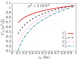
Figure 1: The $z_{3}$ dependence of the Wilson coefficients, $C_{n}(\mu^{2}z^{2}_{3})$, in the leading-twist OPE for transversity for $n=1,2,3$ and $4$. The value of $\mu=\sqrt{2}$ GeV.

The matching relation involving the perturbative kernel ${\cal C}$ has the general form of the lightcone OPE Balitsky and Braun (1989)

$$\mathfrak{M}^{\rm twist-2}(\nu,z_{3}^{2})=\int_{0}^{1}du\,{\cal C}\left(u,\mu^{2}z_{3}^{2}\right){\cal I}(u\nu,\mu),$$ (23)

where the normalized ${\overline{\mathrm{MS}}}$ light-cone transversity ITD ${\cal I}(u\nu,\mu)$ is related to the transversity PDF by

$${\cal I}(\nu,\mu)=\int_{-1}^{1}dx\,e^{ix\nu}\,\frac{h_{u-d}(x,\mu)}{g_{T}(\mu)}.$$ (24)

The expression for the matching kernel at NLO was found to be given by

$${\cal C}(u,\mu^{2}z_{3}^{2})=\delta(1-u)-\frac{\alpha_{s}C_{F}}{2\pi}\bigg{\{}\left[\frac{2u}{1-u}\right]_{+}\ln\left(\frac{z_{3}^{2}\mu^{2}e^{2\gamma_{E}+1}}{4}\right)+4\left[\frac{\ln(1-u)}{1-u}\right]_{+}\bigg{\}}.$$ (25)

Here we use the standard definition of the plus-prescription at $u=1$. The matching formula may also be rewritten Braun and Müller (2008); Izubuchi et al. (2018) in the form of the leading-twist local OPE

$$\mathfrak{M}^{\rm twist-2}(\nu,z_{3}^{2})=\sum_{n=0}^{2N_{\rm max}}a_{n+1}(\mu)C_{n}\left(\mu^{2}z_{3}^{2}\right)\frac{\left(i\nu\right)^{n}}{n!}\ ,$$ (26)

which is nothing but the Taylor expansion in $\nu$ of the lightcone OPE to an order $N_{\rm max}$. The accuracy of the leading-twist local OPE improves as $N_{\rm max}\to\infty$, but a large-enough value of $N_{\rm max}$ is sufficient given the statistical precision of the lattice data, as well as the finite range of $\nu$ and $z_{3}$ that the lattice data spans. The Mellin moments normalized by $g_{T}(\mu)$ are given by

$$a_{n+1}(\mu)=\begin{cases}{\langle x^{n}\rangle_{-}}/{g_{T}},\quad\text{even\ }n,\cr{\langle x^{n}\rangle_{+}}/{g_{T}},\quad\text{odd\ }n,\end{cases}$$ (27)

with $a_{1}(\mu)=1$. The leading-twist NLO Wilson coefficients, $C_{n}(\mu^{2}z_{3}^{2})=\int_{0}^{1}du\,{\cal C}(u,\mu^{2}z_{3}^{2})u^{n}$, for transversity are given by

$$C_{n}\left(\mu^{2}z_{3}^{2}\right)=1+\frac{\alpha_{s}C_{F}}{\pi}\bigg{\{}\ln\left(\frac{z_{3}^{2}\mu^{2}e^{2\gamma_{E}+1}}{4}\right)\sum_{k=2}^{n+1}\frac{1}{k}-\left(\sum_{k=1}^{n}\frac{1}{k}\right)^{2}-\sum_{k=1}^{n}\frac{1}{k^{2}}\bigg{\}}\ .$$ (28)

By fitting the lattice data for ${\rm Re}\,\mathfrak{M}$ using the above expression for ${\rm Re}\,\mathfrak{M}^{\rm twist-2}$, we can obtain $h_{-}(x,\mu)$. Similarly, we can obtain $h_{+}(x,\mu)$ from ${\rm Im}\,\mathfrak{M}$. We use the value of $\alpha_{s}$ from the PDG Tanabashi et al. (2018) at the same scale $\mu$ used to determine the PDF.

In Fig. 1, we show the variation of the Wilson coefficients $C_{n}$ with $z_{3}^{2}$ at a scale of $\mu=\sqrt{2}$ GeV. As the Mellin moments typically decrease rapidly with the order $n$, and also due to the $n!$ suppression of higher-orders in Eq. (26), only the few lowest $n$ mainly contribute in Eq. (26) given a finite range in $\nu$. Therefore, Fig. 1 shows the effect of $O(\alpha_{s})$ corrections to $C_{n}$ for the lowest four $n$. The 1-loop effect on $C_{1}$ and $C_{2}$ at intermediate $z_{3}\approx 0.4$ fm is about 10% and 20% respectively, whereas the effect is about 35% on $C_{3}$ and $C_{4}$. For even smaller $z_{3}$ where the effect of $\ln(\mu^{2}z_{3}^{2})$ increases, typically only the $n=1$ and 2 dominate Eq. (26), for which the 1-loop effect is about 20% and 40% respectively at $z_{3}=0.2$ fm which is about two lattice units in the ensemble we use for this work. Practically, such ${\cal O}(\alpha_{s})$ corrections could have an even smaller effect when convoluted with realistic PDFs. Thus, at the level of matching, we are working in a region of $z_{3}$ where the 1-loop corrections at a fixed $\alpha_{s}(\sqrt{2}{\ \rm GeV})$ are small.

III Lattice setup

The computation presented in this paper was performed using a lattice ensemble generated by the JLab/W&M/LANL collaboration Edwards et al. (2016) with a lattice spacing $a=0.094$ fm and the pion mass tuned to $M_{\pi}=358$ MeV with a physical strange quark mass. The computation is unitary using 2+1 flavor isotropic Wilson-clover fermion action in both the sea and the valence quark sectors. We used a fixed lattice size of $L^{3}\times L_{t}=32^{3}\times 64$. Further details of the ensemble are presented in Refs. Yoon et al. (2017, 2016).

In order to project onto the nucleon ground-state $|P,S_{\perp}\rangle$ with spatial momentum $\mathbf{P}=(0,0,P_{3})$ and with the spin polarization $S^{\perp}$ that is in a spatial direction $\nu$, perpendicular to $\mathbf{P}$, we insert the nucleon interpolating operator ${\cal N}(t^{\prime},P_{3},S^{\perp})$ in time-slices $t^{\prime}=t$ and $t^{\prime}=0$. The key features of this computation are the usages of distillation Peardon et al. (2009) and its modification using phases Egerer et al. (2021b) that make determination of high-momentum matrix elements possible. The details related to the implementation of distillation, that is pertinent to the ensemble used here, is given in our previous publication Egerer et al. (2021a). The spin projection is achieved via the projectors ${\cal P}^{\perp}=\frac{1}{2}(1+\gamma_{5}\not{S}^{\perp})=\frac{1}{2}(1+\gamma_{5}\gamma_{\nu})$. In the Pauli-Dirac representation we use in our computations, the spin projector for the positive parity state reduces to a more familiar $2\times 2$ matrix, ${\cal P}^{\perp}=\frac{1}{2}(1+\sigma_{\nu})$. We computed the set of spatial momenta,

$$P_{3}=n_{3}\Delta;\qquad\Delta=\frac{2\pi}{La}=0.41{\rm\ GeV},$$ (29)

for $n_{3}=0,1,2,3,4,5,6$. In physical units, these momenta correspond to $P_{3}=0,0.41,0.82,1.23,1.64,2.06$ and 2.47 GeV respectively. For the sake of lattice corrections, the pertinent scale is $a^{-1}$, in units of which these momenta correspond to $0.196n_{z}$; that is, the lowest four momenta are well below $a^{-1}$, where as the highest two momenta are comparable to $a^{-1}$.

We extracted the bare matrix element ${\cal M}(z_{3},P_{3})$ by computing the two-point function,

$$C_{\rm 2pt}(t_{s};P_{3})=\left\langle{\cal N}(t_{s},-P_{3},S^{\perp})\overline{\cal N}(0,P_{3},S^{\perp})\right\rangle,$$ (30)

and the three-point function,

$$C_{\rm 3pt}(t_{s},\tau;z_{3},P_{3})=\frac{1}{2}\sum_{\rho=1}^{2}\left\langle{\cal N}(t_{s},-P_{3},S^{\perp})O_{\gamma_{5}\gamma_{0}\gamma_{\rho}}(z_{3};\tau)\overline{\cal N}(0,P_{3},S^{\perp})\right\rangle,$$ (31)

where the operator $O_{\gamma_{5}\gamma_{0}\gamma_{\rho}}(z_{3};\tau)$ is inserted at a time-slice $\tau$, for $0<\tau<t_{s}$. We used $t_{s}=4a,6a,8a,10a,12a,14a$ in our computation. In physical units, the source-sink separation ranges from 0.388 fm to 1.358 fm. As we will see, at the three highest momenta, reasonable signal was obtained up to $t_{s}=10a$ corresponding to 0.97 fm. Our values of quark-antiquark separations $z_{3}$ ranged from $0$ to $16a$ for momenta $n_{3}<4$, and ranged from $0$ to $8a$ for the higher three momenta. Since, we performed fits in shorter $z_{3}<1$ fm, only the values of $z_{3}\leq 10a$ were actually usable in the analysis. In Eq. (31), we have averaged over the two spatial directions that are transverse to $P_{3}$, but we checked to ensure that the two individual three point functions are consistent with each other well within 1-$\sigma$ errors.

IV Extraction of bare matrix element

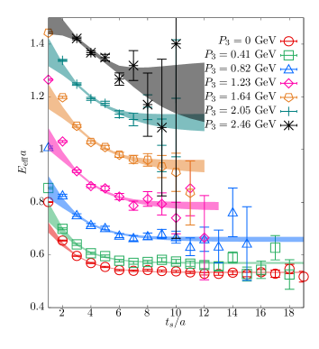
Figure 2: The effective masses $E_{\rm eff}(t_{s})$ determined from the two-point function of transversely polarized nucleon at different momenta $P_{3}$ along the $z$-direction are shown as a function of source-sink separation $t_{s}/a$. The filled bands are the expectations for $E_{\rm eff}(t_{s})$ based on the two-state fits to the nucleon correlator over a fit range $t_{s}\in[3a,18a]$.

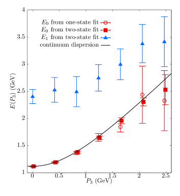
Figure 3: The plot shows the ground state nucleon energy, $E_{0}$, (filled red squares) and the first excited state, $E_{1}$, (filled blue triangles) as extracted from the nucleon two-point function using the two-state fits over a range $t_{s}\in[3a,18a]$, at different nucleon momenta $P_{3}$. For comparison, the nucleon ground state masses obtained from the one-state fits over a range of $t_{s}\in[10a,18a]$ are shown using the open red circle symbols.

We follow the standard ways to obtain the bare matrix element from the three-point and two-point functions in Eq. (30) and Eq. (31); namely, two-state fits to the ratio of three-point to two-point functions and via summation method Maiani et al. (1987); Capitani et al. (2012). In the end, we will primarily use the summation method to cross-check the consistency of the extrapolations from the two-state fits of the ratio, and input the extrapolated matrix elements from the three-point to two-point ratio in the analysis of transversity PDF in the rest of the paper.

For the fits, we use the spectral decomposition of the two-point and three-point functions in terms of the excited-state energies $E_{n}$ and their amplitudes $Z_{n}$, namely,

$$C_{\rm 2pt}(t_{s};P_{3})=\sum_{n=0}^{N-1}|Z_{n}|^{2}e^{-E_{n}t_{s}};\qquad Z_{n}=\frac{1}{\sqrt{2E_{n}}}\langle 0|{\cal N}|n\rangle,$$ (32)

and

$$C_{\rm 3pt}(t_{s},\tau;z_{3},P_{3})=\sum_{n,m=0}^{N-1}\frac{Z_{n}^{*}Z_{m}}{2\sqrt{E_{n}E_{m}}}\langle n|O(z_{3})|m\rangle e^{-E_{n}(t_{s}-\tau)-E_{m}\tau}.$$ (33)

It is clear that the leading ground-state contribution in $C_{\rm 3pt}$ is the desired ${\cal M}(z_{3},P_{3})$. Given the statistical error in the data, we truncated the above spectral decomposition at $N=2$ in both Eq. (32) and Eq. (33); we refer to fits performed with this $N=2$ truncation as the two-state fits. Our methodology is to use the two-state fits using Eq. (32) to obtain the energies and amplitudes of the nucleon and the first excited state from the two-point function data. Using the jackknife samples of fitted values as the input, we then performed two-state fits to the $t_{s}$- and $\tau$-dependencies of the three-point function data using the matrix elements, $\langle n|O(z_{3})|m\rangle$, as the fit parameters. The resultant jackknife samples of the fitted values of the ground-state matrix element, ${\cal M}(z_{3},P_{3})$, were then used in the analysis of transversity PDF that we will discuss in the following sections. It is convenient to implement this excited-state analysis scheme by defining the ratio,

$$R(t_{s},\tau;z_{3},P_{3})\equiv\frac{C_{\rm 3pt}(t_{s},\tau;z_{3},P_{3})}{C_{\rm 2pt}(t_{s};P_{3})},$$ (34)

so that the leading term in its corresponding spectral decomposition that follows from Eq. (32) and Eq. (33) is simply the bare matrix element ${\cal M}(z_{3},P_{3})$. A related technique is the summation method, which uses the quantity,

$$R^{\rm sum}(t_{s};z_{3},P_{3})=\sum_{\tau=\tau_{0}}^{t_{s}-\tau_{0}}R(t_{s},\tau;z_{3},P_{3}),$$ (35)

where one can skip $\tau_{0}$ data points closer to the source and the sink. From the spectral decomposition, it is clear that the leading $t_{s}$ dependence is a straight-line,

$$R^{\rm sum}(t_{s};z_{3},P_{3})=t_{s}{\cal M}(z_{3},P_{3})+R_{0}+{\cal O}\left(e^{-(E_{1}-E_{0})t_{s}}\right).$$ (36)

In the $t_{s}\to\infty$ limit, one would expect $t^{-1}_{s}R^{\rm sum}(t_{s})$ to approach ${\cal M}$.

We used ($N=1$) one-state and ($N=2$) two-state fits to the nucleon two-point function to extract the ground-state energy $E_{0}(P_{3})$. We varied the fit range $t_{s}\in[t_{\rm min},t_{\rm max}]$ to check for the robustness of the fit parameters. For the one-state fits, we found using a fit range $[10a,18a]$ to be optimal and be consistent with the larger $t_{\rm min}$. For $P_{3}=0$, we found the nucleon mass in the ensemble to be 1.115(5) GeV. As a cross-check, the estimate for nucleon mass here using a single interpolating operator is consistent with an earlier estimate Khan et al. (2021b) on the same ensemble using an extensive GEVP basis. Since, we use values of $t_{s}$ and $\tau$ which are smaller than $10a$, a single-state fit is not a feasible approach to obtain the matrix elements, and therefore, we performed two-state fits to the nucleon correlator with smaller values of $t_{\rm min}=2a,3a$ and $4a$, and $t_{\rm max}=18a$. At all the momenta, we found that such two-state fits resulted in $E_{0}$ that were consistent with those obtained using one-state fits with $t_{\rm min}\geq 10a$. It was also encouraging that the central values of $E_{0}$ and $E_{1}$ obtained from the two-state fits, showed only small variations ($<1\%$ for $E_{0}$ and $<10\%$ for $E_{1}$) when $t_{\rm min}$ was changed and such variations were within the statistical errors. Therefore, we used the results of two-state fits over a range $[3a,18a]$ in the extrapolation of three-state fits to be discussed next. In Fig. 2, we show the effective mass, $E_{\rm eff}(t_{s})$, as a function of source-sink separation, $t_{s}$. In the figure, we have differentiated the data at different $P_{3}$ using different colored symbols as specified in the legend. We have compared the expectation for $E_{\rm eff}(t_{s})$ from the two-state fits, shown as the bands of different colors for different $P_{3}$, with the actual data for $E_{\rm eff}$. The goodness of the two-state fits is evident in the agreement with the data for $t_{s}\geq 3a$.

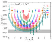
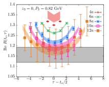
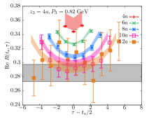
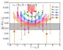
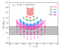
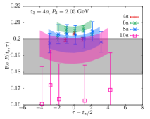
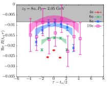
Figure 4: The plot shows a sample of the excited-state extrapolations of the ratio $R(t_{s},\tau)$ of the three-point function to two-point function ratio to obtain the bare ground-state nucleon matrix element, ${\cal M}(z_{3},P_{3})$. As the real and imaginary parts of $R$ displayed similar behaviors, only the real part of $R$ is shown. In each panel, ${\rm Re\ }R(t_{s},\tau)$ is shown as a function of $t_{s}-\tau/2$, where $t_{s}$ is the source-sink separation and $\tau$ is the operator insertion time. The points are the lattice measurements and the bands are the expectations based on the two-state fits to ${\rm Re\ }R(t_{s},\tau)$ over a range of $t_{s}\in[6a,14a]$. The ratios at different fixed $t_{s}$, as specified in the plot legends, are distinguished by the colored symbols and bands used. The horizontal gray band is the extrapolated value. The matrix of panels are such that the three rows from the top to bottom show the results at momenta $P_{3}=0,0.82$ and 2.05 GeV, and the three columns from the left to right are for quark-antiquark separations $z_{3}=0,4a$ and $8a$ respectively.

In Fig. 3, we show the dispersion relation for the ground state and the excited state. For the ground state, we have shown the consistency between the results for $E_{0}(P_{3})$ from the two-state fits with those from the one-state fits. The black curve is the expected continuum single particle dispersion $E_{0}=\sqrt{M_{N}^{2}+P_{3}^{2}}$ with $M_{N}=1.115$ GeV. The fitted data for $E_{0}(P_{3})$ agrees with the continuum dispersion over the entire range of $P_{3}$, with only a slight tendency for the central values of $E_{0}(P_{3})$ to be smaller than the continuum values at the largest three momenta, which could be an effect of a small lattice correction, specifically an $\mathcal{O}\left(a^{2}P_{z}^{2}\right)$ error. We have also shown the dispersion of the first excited state as the blue triangles. At $P_{3}=0$, the gap $E_{1}-E_{0}=1.3(2)$ GeV is larger than the expectation that the leading excitation are $N\pi\pi$ multi-particle state, for which the gap is about 0.7 GeV. This suggests that the first excited state from our two-state fits only effectively captures the tower of excited states above the ground-state nucleon.

Using the spectral content data from the two-state analysis of the nucleon two-point function, we performed the extrapolation of the real and imaginary parts of $R(t_{s},\tau)$ using two-state fits to obtain ${\cal M}(z_{3},P_{3})$. For the two-states, there are four independent parameters (i.e., the matrix elements) as the fit parameters for each of the real and imaginary parts of $R$. For the fits, we skipped the shortest $t_{s}=4a$ and used only $t_{s}\in[6a,14a]$, and for each $t_{s}$, we used only the operator insertion time values $2a\leq\tau\leq t_{s}-2a$ to reduce any end-point effects. Thus, the number of data points being fit is 35 for the choice of fit range using 4 parameters, albeit with correlated data points and with larger $t_{s}>10a$ being noisy for the largest two momenta effectively reduces the number of data points being fit. In our fits, we included the correlations between the data points at a given $t_{s}$ and also the cross-correlations at different $t_{s}$. We found the correlated $\chi^{2}/{\rm dof}$ to vary in the acceptable range around 1 for all the cases studied here. In Fig. 4, we show some sample two-state fits to ${\rm Re\ }R(t_{s},\tau;z_{3},P_{3})$ at $P_{3}=0,0.82$ and 2.05 GeV, and for $z_{3}=0,4a$ and $8a$. In addition to the data for $R$ and the bands resulting from the two-state fits, we also show the extrapolated value for ${\cal M}(z_{3},P_{3})$ as the grey band in the different panels. From the figure, it is clear that at the lower momenta where the data at all $t_{s}$ are well-determined, the two-state extrapolation describes the ratio data well. For the intermediate momenta around 0.82 GeV, the data for $t_{s}>10a$ become noisy and do not contribute to the fits. For the largest two momenta, as seen in the example $P_{3}=2.05$ GeV data shown in the figure, the fits are constrained mainly by the $t_{s}=6a$ and $8a$ source-sink separations.

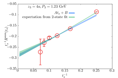
Figure 5: Extraction of the ground state matrix element by using the summation method via fits to $R^{\rm sum}(t_{s})$. The plot shows $t_{s}^{-1}R^{\rm sum}(t_{s})$ as a function of $t_{s}^{-1}$, defined conveniently such that the $y$-intercept at $t_{s}\to\infty$ is the ground-state matrix element, ${\cal M}$. The data points for $R^{\rm sum}(t_{s})$ at a fixed $P_{3}=1.23$ GeV and $z_{3}=4a$ are shown as the red circles. The resulting curve from the straight-line fit to $R^{\rm sum}(t_{s})={\cal M}t_{s}+B$ over a range $t_{s}\in[6a,16a]$ is shown as the blue band. The expectation for $R^{\rm sum}(t_{s})$ from the two-state fits to the ratio $R(t_{s},\tau)$ over a range $t_{s}\in[6a,16a]$ is shown as the green band.

We performed further consistency check on our two-state extrapolations by using summation method to determine ${\cal M}(z_{3},P_{3})$. For this, we fitted the straight-line in Eq. (36) to the $t_{s}$ dependence of the lattice data for $R^{\rm sum}(t_{s};z_{3},P_{3})$. We used $\tau_{0}=2a$ to skip the end-points to find $R^{\rm sum}$, but changing its value was not crucial. We did the straight-line fits over the range of $t_{s}\in[6a,14a]$; the deterioration of signal for $R^{\rm sum}(t_{s})$ at larger $t_{s}$ with increasing $P_{3}$ followed the same trend as we explained above for the ratio $R$. In Fig. 5, we have shown a sample straight-line fit to $R^{\rm sum}(t_{s})$ at $P_{3}=1.23$ GeV and $z_{3}=4a$. The $y$-axis in Fig. 5 is $t_{s}^{-1}R^{\rm sum}(t_{s})$ and the $x$-axis is $t_{s}^{-1}$, such that when $t_{s}^{-1}=0$, the $y$-intercept will give the value of ground-state matrix element. The blue-band is the result from the straight-line fit over $t_{s}\in[6a,14a]$, which passes through all the data points satisfactorily, and not surprisingly, misses the data point at the smallest $t_{s}=4a$ which did not enter the fit. For comparison, we also show the expectation for $t_{s}^{-1}R^{\rm sum}(t_{s})$ from the two-state fits to the ratio $R(t_{s},\tau)$ over $t_{s}\in[6a,14a]$, that we discussed previously, as the green band. The two estimates for ${\cal M}$ are consistent within error-bars as seen from the $y$-intercepts of the two bands, validating the extrapolations at least for the specific $(z_{3},P_{3})$ shown in the figure. However, the surprising feature in Fig. 5 (and also for other $(z_{3},P_{3})$ as well), is that the expected curve for $R^{\rm sum}(t_{s})$ from the two-state fit always passes through the $t_{s}=4a$ data point as well, unlike the summation fit curve. This seems to suggest that the two-state fit has a slight advantage from the sensitivity to the tower of higher excited states captured through the effective first excited state $E_{1}$. We attempted to test the robustness of summation fits by supplementing the straight-line fit form with a term proportional to $e^{-(E_{1}-E_{0})t_{s}}$, but it however resulted in unstable fits with large errors in the fit parameters. In the different panels of Fig. 6, we show the results of ${\cal M}(z_{3},P_{3})$ as a function of $z_{3}$ that were obtained from the two-state fit extrapolations (shown using circles) and the summation fit extrapolations (shown using squares), at different $P_{3}$. In each panel, ${\rm Re}{\cal M}$ and ${\rm Im}{\cal M}$ are shown using red and blue symbols respectively. The comparison nicely demonstrates the consistency between the two different ways of extrapolations to get ${\cal M}$, thereby indirectly, justifying a good estimation of the ground state matrix element. Therefore, we will use the bare matrix element obtained from the two-state fit in the rest of the paper, due to its usage of more data points in its fits, especially at the larger $P_{3}$ where the summation fit essentially uses only two data points, as well as due to its good ability to describe even the smaller $t_{s}$ that did not even enter the fits.

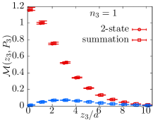
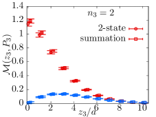
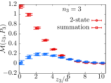
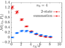
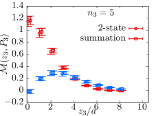
Figure 6: The plot demonstrates the consistency in the extracted bare matrix elements ${\cal M}(z_{3},P_{3})$ by means of comparison between the extrapolated values from two-states fits to $R(t_{s},\tau)$ (circles) and straight-line fits to $R^{\rm sum}(t_{s})$ (squares). The red and blue symbols are for ${\rm Re\ }{\cal M}$ and ${\rm Im\ }{\cal M}$ respectively. The different panels show this comparison at various momenta $P_{3}=0.41n_{3}$ GeV for $n_{3}=0,1,2,3,4,5$.

V A numerical analysis of corrections to continuum leading-twist formalism

The simplest analysis of the lattice pseudo-ITD data, without incorporating any ansatz for the PDF is to use the Mellin moments as the fit parameters, as first introduced in Ref. Karpie et al. (2018). The premise of the calculation is to find the best fit values of the Mellin moments by fitting the Ioffe-time, $\nu$, dependence of the real and imaginary parts of $\mathfrak{M}(\nu,z_{3}^{2})$ using the leading-twist OPE given in Eq. (26) at various fixed values of $z_{3}$. In this way, we can obtain the Mellin moments $\langle x^{n}\rangle_{\pm}$ as a function of $z_{3}$. If the leading-twist OPE at a given perturbative order by itself is sufficient to describe the lattice data in a given range of $z_{3}$ and $\nu$, then we should find no $z_{3}$-dependence in the fitted values of $\langle x^{n}\rangle_{\pm}$. By turning the argument around, by assuming that the NLO leading-twist OPE is sufficient except that it needs to be supplemented by small additional $\nu$ and $z_{3}$ dependent lattice corrections as well as higher-twist corrections, then the moments analysis at fixed $z_{3}$ is a nice way to query the nature of these small corrections. The idea is the following — if the lattice pseudo-ITD data is an admixture of the leading-twist part $\mathfrak{M}^{\rm twist-2}$ and some leading corrections in $1/|z_{3}|$ and $|z_{3}|$, such as,

$$\mathfrak{M}(\nu,z_{3}^{2})=\mathfrak{M}^{\rm twist-2}(\nu,z_{3}^{2})+\sum_{k,n}\left(L_{k,n}\left(\frac{a}{|z_{3}|}\right)^{k}+H_{k,n}\left(\Lambda^{2}_{\rm QCD}z_{3}^{2}\right)^{k}\right)\frac{(i\nu)^{n}}{n!},$$ (37)

for some numerical coefficients $L_{k,n}$ and $H_{p,n}$, then we can absorb the corrections into the leading-twist OPE, which effectively results in a $z_{3}$-dependent $n$-th moment given by,

(38)

$$a^{\rm eff}_{n+1}(z_{3})=\langle x^{n}\rangle+\frac{1}{C_{n}(\mu^{2}z_{3}^{2})}\sum_{k}\left(L_{k,n}\left(\frac{a}{|z_{3}|}\right)^{k}+H_{k,n}\left(\Lambda^{2}_{\rm QCD}z_{3}^{2}\right)^{k}\right).$$ (40)

In practice, since the Wilson coefficients depend on $z_{3}$ logarithmically, one will see some power-law corrections in $1/|z_{3}|$ and $|z_{3}|$ to the moments extracted from OPE-without-OPE analysis, thereby allowing us to deduce what the leading corrections are from the lattice data itself. Also, only corrections with $n>0$ can appear as $a_{1}=1$ by construction. Such an approach was also considered previously in Gao et al. (2020) to deduce the nature of lattice corrections for $z_{3}\sim{\cal O}(a)$. Here, we take a similar stance and ask whether there are corrections to the leading-twist OPE as seen in the Mellin moments, and if so, what is the simplest correction that we need to add to the leading-twist OPE in order to extract the PDF?

At any given $z_{3}$, we only have six data points from the different $P_{3}$. Therefore, we needed to truncate the leading-twist OPE in Eq. (26) at modest values of $N_{\rm max}$ for this analysis of moments; we used $N_{\rm max}=2,3,4$ and checked for the convergence of the results. In the top panels of Fig. 7, we show the results from the moments analysis using $N_{\rm max}=4$ truncation. We used $\mu=\sqrt{2}$ GeV to do the matching and used $\alpha_{s}(\sqrt{2}{\rm GeV})=0.36$ in the Wilson coefficients. The data points in the top-left and top-right panels are our data for ${\rm Im}\mathfrak{M}$ and ${\rm Re}\mathfrak{M}$ respectively. We have differentiated the data at fixed values of $z_{3}$ ranging from $2a$ to $7a$ using different colored symbols. Along with the data points, we show the resulting bands from the fits at each values of $z_{3}$. The fits indeed describe the Ioffe-time dependence as well as the $z_{3}$ dependencies of the lattice data well, albeit at the expense of allowing for $z_{3}$ dependence of the moments as seen in the two bottom panels.

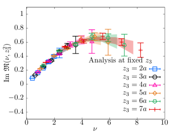
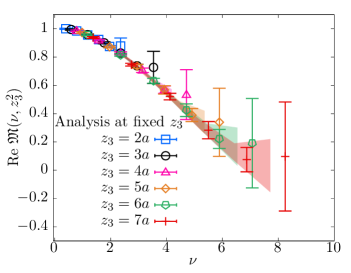
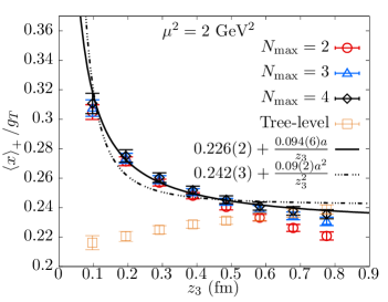
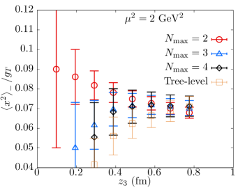
Figure 7: The analysis of $\nu$ dependence at different fixed $z_{3}$. The top-left and top-right panels show ${\rm Im}\mathfrak{M}$ and ${\rm Re}\mathfrak{M}$ as a function of the Ioffe-time, $\nu$. The data points for $\mathfrak{M}(\nu,z_{3}^{2})$ at different fixed $z_{3}$ are differentiated by the colored symbols. The corresponding fits to the leading-twist OPE with $N_{\rm max}$ Mellin moments as the fit parameters, at various fixed values of $z_{3}^{2}$ are the colored bands. In the fits shown in the top panels, $N_{\rm max}=4$ Mellin moments were used. The bottom-left panel shows the corresponding $z_{3}$-dependence of $\langle x\rangle_{+}(\mu)/g_{T}(\mu)$ as obtained from fits to ${\rm Im}\mathfrak{M}(\nu,z^{2})$ at the different fixed $z_{3}^{2}$. The results using the truncation order $N_{\rm max}=2,3,4$ are shown. The black curve is the expectation for the observed residual $z_{3}$ dependence based on a short-distance lattice artifact of the type $L_{1,1}(a/|z_{3}|)\nu$ (refer text). The results from fits using tree-level Wilson coefficients (i.e., $C_{n}=1$) and $N_{\rm max}=4$ are also shown to see the effect of 1-loop matching. A similar $z_{3}$-dependence of $\langle x^{2}\rangle_{-}/g_{T}$ at $\mu=\sqrt{2}$ GeV as obtained from the leading-twist OPE fits to ${\rm Re}\mathfrak{M}(\nu,z_{3}^{2})$ is shown in the bottom-right panel.

The bottom-left and right panels of Fig. 7 show the $z_{3}$ dependencies of the dominant fit parameters in the OPE of ${\rm Re}\mathfrak{M}$ and ${\rm Im}\mathfrak{M}$, namely, the normalized Mellin moments $\langle x\rangle_{+}/g_{T}$ and $\langle x^{2}\rangle_{-}/g_{T}$. Let us first focus on the bottom-left panel in Fig. 7 — the results from the analyses of ${\rm Im}\mathfrak{M}$ using $N_{\rm max}=2,3,4$ are the different colored symbols in the plot. We can infer that by $N_{\rm max}=4$, the fits have more or less converged. The $z_{3}$ dependence of $\langle x\rangle_{+}/g_{T}$ is striking, without any region in the perturbative range of $z_{3}$ that can be identified as a plateau. Thus, it is important to take care of the corrections to the leading twist framework. Since we have analyzed only one ensemble, we have to rely on previous works to deduce the origin of the corrections seen here. We observe that the corrections are larger at shorter $z_{3}$, and hence, suggests that the dominant source of the correction could be due to the lattice corrections when $z_{3}$ is comparable to the lattice cut-off itself. Indeed, a similar observation has been made in previous works Gao et al. (2020); Karpie et al. (2021) that used more than one lattice spacing. Therefore, in this work, we will proceed under the hypothesis that the leading correction is a lattice spacing correction of the type $L_{k,m}\left(a/|z_{3}|\right)^{k}(i\nu)^{m}$ that we discussed above. The solid black curve in the bottom-left panel is a fit using the form $a_{2}^{\rm eff}(z_{3})=\langle x\rangle_{+}/g_{T}+L_{1,1}\left(a/|z_{3}|\right)$, with $\langle x\rangle_{+}/g_{T}=0.226(2)$ and $L_{1,1}=0.094(6)$. On the other hand, a fit to an alternate correction of the type $L_{2,1}\left(a/|z_{3}|\right)^{2}$ performs poorly as seen from the dashed curve shown in the bottom-left panel of Fig. 7. Thus, we infer that the leading correction to ${\rm Im}\mathfrak{M}$ is a correction of the form $L_{1,1}\left(a/|z_{3}|\right)\nu$. In addition to the lattice correction, we do not find any perceptible higher twist corrections of the form $(\Lambda_{\rm QCD}|z_{3}|)^{2}\nu$ present in our data for ${\rm Im}\mathfrak{M}$ up to $z_{3}=0.8$ fm, indicating that most of the higher twist effects have presumably canceled between the bare matrix elements ${\cal M}(z_{3},P_{3})$ and ${\cal M}(z_{3},0)$ in their ratio. A similar plot of the effective $a_{3}^{\rm eff}(z_{3})$ as extracted from ${\rm Re}\mathfrak{M}$ is shown on the bottom right panel. Unlike the results on the bottom-left panel, the fitted values of $a_{3}^{\rm eff}(z_{3})$ are comparatively noisier, especially at the shorter $z_{3}<0.4$ fm. For $z_{3}>0.4$ fm up to 0.8 fm, a plateau is seen. Thus, to the precision of the data, we found no indications of small-distance lattice correction nor any higher-twist corrections in ${\rm Re}\mathfrak{M}$. To see the effect of DGLAP as enshrined in the $\ln(\mu^{2}z_{3}^{2})$ in the NLO Wilson coefficients, we also performed the above analysis using the tree-level matching as obtained using $\alpha_{s}=0$ and therefore lacks the logarithmic part as well as some finite $\alpha_{s}$ corrections (the resulting tree-level moments can also be inferred as the moments of the pseudo-ITD). From the bottom panels, we see that the effect of 1-loop is quite important for the ${\rm Im}\mathfrak{M}$ compared to ${\rm Re}\mathfrak{M}$. From the $z_{3}$ behavior for $\langle x\rangle_{+}$, we see that the effect of DGLAP and the effect of the $a/z_{3}$ lattice correction have opposing behaviors, and taking care of the them together is important in lattice studies at finite lattice spacings.

Based on the above analysis, the explicit functional forms for the leading-twist OPE along with the simplest leading lattice-spacing correction and higher-twist correction, that we will use in the extraction of the $x$-dependent PDF in the remaining part of the paper is

$${\rm Re}\left(\mathfrak{M}\left(\nu,z_{3}^{2}\right)\right)=\left(1+\sum_{n=1}^{N_{\rm max}}C_{2n}\left(z_{3}^{2}\mu^{2}\right)\frac{(-1)^{n}\nu^{2n}}{(2n)!}\int_{0}^{1}x^{2n}\frac{h_{-}(x,\mu)}{g_{T}(\mu)}dx\right)+L_{1,2}\frac{a}{|z_{3}|}\frac{\nu^{2}}{2}+H_{1,2}\left(\Lambda_{\rm QCD}z_{3}\right)^{2}\frac{\nu^{2}}{2},$$ (41)

and for the imaginary part is,

$${\rm Im}\left(\mathfrak{M}\left(\nu,z_{3}^{2}\right)\right)=\left(\sum_{n=1}^{N_{\rm max}}C_{2n-1}\left(z_{3}^{2}\mu^{2}\right)\frac{(-1)^{n-1}\nu^{2n-1}}{(2n-1)!}\int_{0}^{1}x^{2n-1}\frac{h_{+}(x,\mu)}{g_{T}(\mu)}dx\right)+L_{1,1}\frac{a}{|z_{3}|}\nu+H_{1,1}\left(\Lambda_{\rm QCD}z_{3}\right)^{2}\nu,$$ (42)

with the terms within the larger parentheses in the above expression are simply the convolution term in Eq. (23) expanded in $\nu$ for convenience in implementation. We will use a value ${\Lambda_{\rm QCD}}=0.286$ GeV as a typical scale simply to get dimensionless values above. We found actual evidence in the data only for a non-zero $L_{1,1}$ in the imaginary part, and whereas, we have added the other correction terms, namely $L_{1,2}$, $H_{1,1}$ and $H_{1,2}$, in order to be conservative in our fits and also because there is no a priori reason for the absence of such leading lattice correction terms or the higher-twist correction terms. In the end, we found such terms to come out with values close to zero, which we will take as an empirical fact. We should also note that the lattice correction term $L_{1,2}$ in the real part is proportional to the modulus $|z_{3}|^{-1}$. This is in contrast to Ref. Gao et al. (2020) for the analysis of pion valence PDF, where an analytic correction term $(a/z_{3})^{2}\nu^{2}$ was used for ${\rm Re}\mathfrak{M}$ due to visible evidence for such a term in the data. In our case, there is no such visible evidence for ${\rm Re}\mathfrak{M}$ data, and therefore, we add a term with lesser power of $|z_{3}|^{-1}$, which in principle could be present. Such an approach was also taken for the case of the analysis for the nucleon unpolarized PDF Karpie et al. (2021); Egerer et al. (2021a). We also cross-checked by adding $(a/z_{3})^{2}\nu^{2}$ as a correction term instead of $(a/|z_{3}|)\nu^{2}$ term to the real part in our studies, but it did not make any statistically significant variation. Therefore, we will present the results with $L_{1,2}$ term in the real part.

We should note that one may parameterize the $\nu$ dependence of both the higher-twist as well as the lattice spacing errors with a more general form. In computations of the nucleon unpolarized PDFs Karpie et al. (2021); Egerer et al. (2021a); Khan et al. (2021a), Jacobi polynomials were used to describe the general $\nu$ dependence of correction terms. However, for the transversity rpITD data presented here, we found the results from an analysis using the Jacobi polynomial parametrization of corrections to leading-twist OPE to be consistent with the results using a simpler parametrization using leading correction terms given above, and hence, we resort to this simpler parametrization in the rest of the paper. Perhaps, an increased precision in the future might necessitate more elaborate terms in the corrections.

VI Reconstruction of transversity PDF with reduced model-dependence

Having set up the required elements for the PDF analysis, we present the results on the extraction of the PDF from the transversity pseudo-ITD in this section. Our approach is to reconstruct the $x$-dependent transversity PDFs, $h_{\pm}(x)$ by assuming a functional form for them, say $h_{\pm}(x;\{\alpha,\ldots\})$, and then perform a combined fit of the parameters $\{\alpha,\ldots\}$ to the $\nu$ and $z_{3}$ dependencies of the pseudo-ITD lattice data over a range of $P_{3}\in[P_{3}^{\rm min},P_{3}^{\rm max}]$ and $z_{3}\in[z_{3}^{\rm min},z_{3}^{\rm max}]$ using Eq. (41) and Eq. (42). As we will explain, through a step by step generalization of the functional form of the PDF ansatz, we reduce the model-dependence. Our fitting method is by using the standard $\chi^{2}$ minimization,

(43)

$$\chi^{2}=\sum_{p,p^{\prime}}\Delta_{p}\Sigma^{-1}_{p,p^{\prime}}\Delta_{p^{\prime}};\quad p=[z_{3},P_{3}],$$ (44)

$$z_{3}\in[z_{3}^{\rm min},z_{3}^{\rm max}],\quad P_{3}\in[P_{3}^{\rm min},P_{3}^{\rm max}],$$ (45)

(46)

where $\Delta_{p}={\rm Re}/{\rm Im}\mathfrak{M}_{\rm data}(p)-{\rm Re}/{\rm Im}\mathfrak{M}_{\rm fit}(p;\{\alpha,\ldots\})$, and $\Sigma_{p,p^{\prime}}$ is the covariance between the different data points $p,p^{\prime}$. The covariance matrix uses its standard definition using only statistical fluctuations, without folding any of the systematic errors into it. We will take care of the systematic variations in the fits in the end.

We used all the six available values of $P_{3}\in[0,2.46]$ GeV in our analysis. However, we were cautious about the range of $z_{3}$ to use; too small values of $z_{3}$ will suffer from larger lattice spacing corrections as we discussed in the last section, whereas for $z_{3}\sim O(1)$ fm, we naively expect higher-twist effects and higher-order perturbative terms could become important. For this, we skipped $z_{3}=0,a$ from our analysis and used only ranges with $z_{3}^{\rm min}=2a,3a$. To see the variations due to the choice of $z_{3}^{\rm max}$, we used $z_{3}^{\rm max}=8a,10a=0.75,0.94$ fm. We used the fixed order expressions for the Wilson coefficients in Eq. (28) at a factorization scale of $\mu=\sqrt{2}$ GeV in our PDF analysis, that is comparable to $1/z_{3}$ that enters our computation.

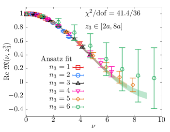
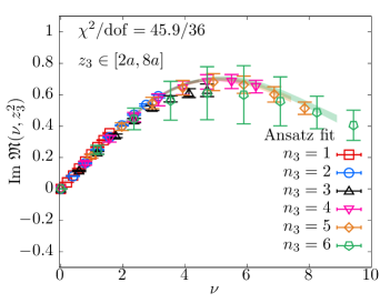
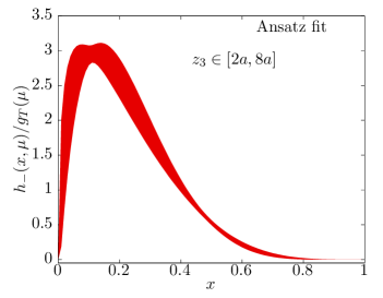
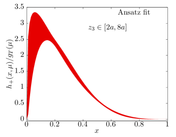
Figure 8: Reconstruction of transversity PDF based on the PDF ansatz in Eq. (47). The top-left and top-right panels show the real and imaginary parts of $\mathfrak{M}$ as a function of $\nu$. The two panels show the best fit bands resulting from an analysis assuming the PDF ansatz. The fits shown in the figure incorporated the data points at all momenta with $z_{3}\in[2a,8a]$. The color of the bands and the data points distinguish the fixed value of momenta $P_{3}=0.41n_{3}$ GeV used. The bottom-left and bottom-right panels show the resultant transversity PDFs, $h_{-}(x)$ and $h_{+}(x)$ respectively.

In the first step of the PDF reconstruction, we assumed a functional form that is known to work well in the global fits to the PDFs from experimental cross-sections data, namely,

$$\frac{h_{\pm}(x)}{g_{T}}=N_{\pm}x^{\alpha_{\pm}}(1-x)^{\beta_{\pm}}\left(1+\gamma_{\pm}\sqrt{x}+\delta_{\pm}x\right),$$ (47)

with $(\alpha_{\pm},\beta_{\pm},\gamma_{\pm},\delta_{\pm})$ as independent fit parameters. The parameter $N_{\pm}$ is the normalizing constant. We will simply refer this method as PDF ansatz fits. For the valence case, $\int_{0}^{1}dx\frac{h_{-}(x)}{g_{T}}=1$, which thereby fixes $N_{-}=N_{-}(\alpha_{-},\beta_{-},\gamma_{-},\delta_{-})$ as a function of the other independent parameters. On the other hand, for $N_{+}$ there is no such condition and therefore, we keep it as an additional fit parameter in $h_{+}/g_{T}$. We used the above functional form in Eq. (41) and Eq. (42) to fit our transversity pseudo-ITD data. We evaluated the convolution integral for the leading-twist matching using the Taylor series in $\nu$ (see Eq. (41) and Eq. (42)) using an expansion up to order $N_{\rm max}=40$. This truncation achieves a machine precision approximation of the convolution kernel within the range of $\nu$ we use.

In the top left and right panels of Fig. 8, we compare our PDF ansatz fit with the real and imaginary parts of our lattice pseudo-ITD data in the left and right panels respectively. For the fits shown in the two panels, we used the fitting ranges $z_{3}\in[2a,8a(0.75{\ \rm fm})]$ and $P_{3}\in[0,2.46{\ \rm GeV}]$. We have represented the data points and fitted bands at a fixed $P_{3}$ by the same set of colors. The data points at different $P_{3}$ and $z_{3}$ quite nicely fall on near universal curves as a function of $\nu$, which means that the scaling violations to the tree-level universality could be described by small perturbative logarithmic terms. Indeed, it is clear from the two panels that the corresponding fitted bands describe the data at different $P_{3}$ well over the range of $z_{3}$ we used. Taking this range of fitted data as a representative point for the sake of discussion, we found the following set of parameters that enter the PDF ansatz:

(48)

$$\alpha_{+}=0.49(42);\qquad\alpha_{-}=0.63(50)$$ (49)

$$\beta_{+}=3.38(1.15);\qquad\beta_{-}=4.37(1.75)$$ (50)

$$\gamma_{+}=-0.28(1.92);\qquad\gamma_{-}=-0.16(2.29)$$ (51)

$$\delta_{+}=-0.30(1.33);\qquad\delta_{-}=-0.17(1.75)$$ (52)

$$N_{+}=10.85(92);\qquad$$ (53)

$$L_{1,1}=0.0648(38);\qquad L_{1,2}=-0.038(20)$$ (54)

$$H_{1,1}=-2.50(2.62)10^{-3};\qquad H_{1,2}=1.86(1.34)10^{-3}$$ (55)

$$\chi^{2}/{\rm dof}=45.9/35;\qquad\chi^{2}/{\rm dof}=41.5/36\ .$$ (56)

(57)

In the bottom-left and right panels of Fig. 8, we show the corresponding best fit transversity PDFs, $h_{-}$ and $h_{+}$, respectively for the representative values of fit ranges; in the last half of this section, we will discuss more on the variability of the fits as a systematic effect. The quality of the fits are acceptable as seen from the $\chi^{2}/{\rm dof}\approx 1.2$. For both $h_{\pm}$, a simpler two-parameter ansatz using only the exponents $(\alpha_{\pm},\beta_{\pm})$ was also sufficient to capture the shape of the transversity PDF, as one can see by the nearly vanishing values of the small-$x$ corrections $\gamma_{\pm}$ and $\delta_{\pm}$. The role of the lattice correction $L_{1,1}$ in ${\rm Im}\mathfrak{M}$ is not negligible as we discussed in the last section, and such a term is necessary to obtain acceptable $\chi^{2}$. Its real counterpart $L_{1,2}$ is comparatively smaller and consistent with zero at 2-$\sigma$ level. The additive higher-twist corrections $H_{1,1}$ and $H_{1,2}$ come out unimportant, and supports an explanation that there are cancellations of higher-twist corrections due to the ratio of nucleon matrix elements in Eq. (22). The fact that $\alpha_{\pm}>0$ results in the transversity PDFs vanishing at $x=0$ in the bottom panels. The region of $x\in[0.1,0.8]$ where the transversity PDF is significantly non-zero could perhaps help their lattice determinations with lesser higher-twist contamination, which is suggested Braun et al. (2019) to affect the $x\approx 0$ and $x\approx 1$ parts of the extracted PDF.

At this point, we are concerned about the robustness of the reconstructed transversity PDFs; by assuming a PDF ansatz, have we inadvertently restricted the set of allowed PDFs severely and ruled out a wider possibility of solutions? The answer to this question can only be found by an actual inversion of the matching relation, and equivalently an inversion of Eq. (41) and Eq. (42), to determine $h_{\pm}(x)$ using a discrete set of data points that span a finite range of $\nu$ and $z_{3}$. This is well known to be an ill-posed problem Karpie et al. (2019). Given the assumption (that is, our prior) that the transversity PDF can be described using the PDF ansatz in Eq. (47) to a good accuracy, and allowing for small fluctuations around this prior, we ask whether we can reconstruct the transversity PDFs using a more flexible PDF parametrization that covers all such possible small fluctuations. We describe our method to answer this question in our ensuing discussion on the reconstruction of the transversity PDF using Jacobi polynomials that form a compete basis of functions of $x$ for $x\in[0,1]$.

The effectiveness of a Jacobi polynomial basis as an easy-to-implement and complete set of functions for $x\in[0,1]$ was first investigated in Ref. Karpie et al. (2021). The reader can refer to Ref. Egerer et al. (2021a) for a more detailed description of a related procedure as applied to the unpolarized PDF. The essential properties of the Jacobi polynomials that we need for this paper are as follows. Any pair of parameters $(\alpha,\beta)$ defines a family of Jacobi polynomials, which we represent as $P_{n}^{\alpha,\beta}(u)$ for $u\in[-1,1]$ which are orthogonal with respect to a weight function $W^{\alpha,\beta}(u)=(1-u)^{\alpha}(1+u)^{\beta}$. We can conveniently rewrite the polynomials as $P_{n}^{\alpha,\beta}(1-2x)$ which span the interval $x\in[0,1]$ that our PDFs are defined in, and with the weight-function as $W^{\alpha,\beta}(x)=x^{\alpha}(1-x)^{\beta}$. That is

$$\int_{0}^{1}P_{n}^{\alpha,\beta}(1-2x)P_{m}^{\alpha,\beta}(1-2x)W^{\alpha,\beta}(x)dx={\cal K}_{n}(\alpha,\beta)\delta_{m,n},$$ (58)

where ${\cal K}_{n}$ is a normalizing constant. Due to this orthogonality of the Jacobi polynomials, we can write the most general functional form for our PDFs as,

(59)

$$h_{\pm}\left(x;\{N_{\pm},\alpha_{\pm},\beta_{\pm},s_{n\pm}\}\right)=N_{\pm}x^{\alpha_{\pm}}(1-x)^{\beta_{\pm}}\left(1+\sum_{n=1}^{N_{J}}s_{n\pm}P^{\alpha_{\pm},\beta_{\pm}}_{n}(1-2x)\right),$$ (60)

$$\quad{\rm with}\quad s_{n}\equiv\frac{1}{{\cal K}_{n}(\alpha,\beta)}\int_{0}^{1}h_{\pm}(x)P^{\alpha_{\pm},\beta_{\pm}}_{n}(1-2x)dx.$$ (61)

(62)

(63)

The above expansion is exact for $N_{J}\to\infty$. While it is tempting to identify $(\alpha_{\pm},\beta_{\pm})$ with the small-$x$ and large-$x$ exponents due to the similarity of the above equation with Eq. (47), such an identification in general is not correct — for this, we note again that $(\alpha_{\pm},\beta_{\pm})$ can be any pair of real numbers, greater that -1, and due to the completeness of the corresponding Jacobi polynomials $P_{n}^{\alpha,\beta}$, the above expansion of $h_{\pm}(x)$ is always exact in the $N_{J}\to\infty$ limit. However, not all choices of $(\alpha_{\pm},\beta_{\pm})$ are numerically optimal when finite $N_{J}$ has to be used, as the above series in $n$ might only slowly converge with $n$, or worse, it might not be uniformly convergent as $n$ is increased unlike, for example, a series in the Chebyshev polynomials. In Refs. Karpie et al. (2021); Egerer et al. (2021a), this convergence problem was approached by finding the best fit values of $(\alpha_{\pm},\beta_{\pm})$ along with the coefficients $s_{n\pm}$ by using the VarPro algorithm Golub and Pereyra (1973).

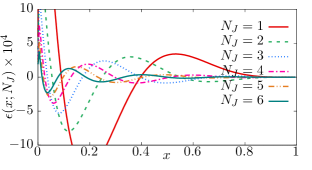
Figure 9: Convergence of the Jacobi polynomial expansion for PDFs that can be described by Eq. (47). The error $\epsilon(x;N_{J})$ due to truncation at order $N_{J}$ (see text) is plotted as a function of $x$. In the example shown, $(\alpha,\beta,\gamma,\delta)=(0.49,3.38,-0.28,-0.3)$ in Eq. (47) for $h_{+}(x)$. The truncation order of the Jacobi polynomial expansion is gradually increased from $N_{J}=1$ to 6 as seen from the different curves.

In this work, we explore another possibility that makes full use of the completeness of Eq. (63) and the empirically known effectiveness of the PDF ansatz in Eq. (47). For this, we specialize the above discussion from a generic $(\alpha,\beta)$ that define $P^{\alpha,\beta}_{n}$ to the case where we identify them with the small-$x$ and large-$x$ exponents. We generalize Eq. (47) and assume that the PDF can be written as

$$h_{\pm}(x)=x^{\alpha_{\pm}}(1-x)^{\beta_{\pm}}{\cal G}_{\pm}(x),$$ (64)

where $\alpha_{\pm}$ and $\beta_{\pm}$ are the actual small-$x$ and large-$x$ exponents, in which case, it is justified to assume that ${\cal G}_{\pm}(x)$ is a slowly-varying function that can be expanded linearly in $P^{\alpha_{\pm},\beta_{\pm}}_{n}$ as

$${\cal G}_{\pm}(x;N_{J})=1+\sum_{n=1}^{N_{J}}s_{n\pm}P^{\alpha_{\pm},\beta_{\pm}}_{n}(1-2x),$$ (65)

with a good convergent behavior as the order of truncation $N_{J}$ in increased. In order to see if this is true, let us consider the central values of $(\alpha_{+},\beta_{+},\gamma_{+},\delta_{+})=(0.49,3.38,-0.28,-0.3)$ from the PDF ansatz in Eq. (47). In this specific example, we would like to see if ${\cal G}_{+}(x)=1-0.28\sqrt{x}-0.3x$ exhibits a convergent behavior with respect to $n$, when it is expanded in the basis $P_{n}^{0.49,3.38}$. Let us define the error committed by the truncation at $N_{J}$ polynomials, $\epsilon(x;N_{J})\equiv x^{\alpha_{+}}(1-x)^{\beta_{+}}\left({\cal G}_{+}(x;\infty)-{\cal G}_{+}(x;N_{J})\right)$. In Fig. 9, we show $\epsilon(x;N_{J})$ as a function of $x$, as $N_{J}$ is increased from 1 to 6 for the example ${\cal G}_{+}(x)$ considered. For the example shown and for similar such four-parameter ansatz parameterizations of the PDF, we found the convergence with $N_{J}$ was uniform over a range $x\in[x_{\rm min},1]$ with $x_{\rm min}$ monotonically becoming smaller with increasing $N_{J}$. Thus, to summarize our observational study of the Jacobi polynomial expansion, at least for PDFs that closely resemble the typical $x^{\alpha}(1-x)^{\beta}$ functional forms, we can consider the Jacobi polynomial expansion of the PDF, using the same values of $\alpha$ and $\beta$ as the small-$x$ and large-$x$ exponents, to be uniformly convergent with $N_{J}$, and it is sufficient to consider only the first few $P_{n}^{\alpha,\beta}$ in the expansion.

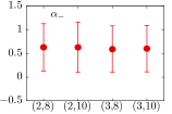
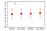
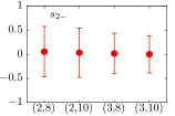
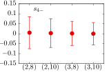
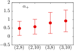
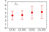
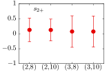
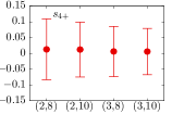
Figure 10: The small-$x$ exponents, $\alpha_{\pm}$, and the large-$x$ exponents, $\beta_{\pm}$, as inferred from the PDF ansatz fits are shown as a function of fit ranges $(z^{\rm min}_{3},z^{\rm max}_{3})$ in the left-half of the figure. The Jacobi polynomial expansion coefficients $s_{2\pm},s_{4\pm}$ obtained from the decomposition of the PDF ansatz fits in a basis $P_{n}^{\alpha_{\pm},\beta_{\pm}}$ are shown as a function of fit ranges in the right-half of the figure. The central values and errors on the inferred expansion coefficients were then fed as prior and prior widths for the fits using the Jacobi polynomial parametrization (see text).

Based on the above discussion, we improved upon our PDF ansatz reconstruction in the following way. Let us denote the parameters and PDFs extracted from the PDF ansatz in Eq. (47) using “ans” in the superscript in the discussion below.

1. For each fit range $z_{3}\in[z_{3}^{\rm min},z_{3}^{\rm max}]$ and $P_{3}\in[P_{3}^{\rm min},P_{3}^{\rm max}]$, we read off the small-$x$ and large-$x$ exponents, $(\alpha_{\pm}^{\rm ans},\beta_{\pm}^{\rm ans})$, from the four-parameter ansatz reconstruction analysis we presented previously. We decomposed the four-parameter PDF that depends on $(\alpha_{\pm}^{\rm ans},\beta_{\pm}^{\rm ans},\gamma_{\pm}^{\rm ans},\delta_{\pm}^{\rm ans})$ into a basis of Jacobi polynomials $P_{n}^{\alpha_{\pm}^{\rm ans},\beta_{\pm}^{\rm ans}}$ using Eq. (63). The output of this decomposition were the expansion coefficients $s_{n\pm}^{\rm ans}$ for any order $n$. By iterating this over jackknife samples of the four-parameter ansatz fits, we estimated the mean $\bar{s}_{n\pm}^{\rm ans}$ and its error $\sigma_{s\pm}^{\rm ans}$ of the expansion coefficients.

2. In the second step, with the same set of fit ranges as in the Step-1, we used the Jacobi polynomial expansion, Eq. (63), truncated at a chosen truncation order $N_{J}$ in Eq. (41) and Eq. (42) with the expansion coefficient $s_{n\pm}$ and the other correction parameters $L_{m,n}$, $H_{m,n}$ as the fit parameters. One should note that the fit is linear in the expansion coefficients $s_{n\pm}$. We imposed our prior that the allowed PDFs are small fluctuations about the PDF ansatz fit, by using the log-likelihood function,

   $${\cal L}=\chi^{2}+\sum_{n=1}^{N_{J}}\left(\frac{s_{n\pm}-\bar{s}^{\rm ans}_{n\pm}}{\sigma^{\rm prior}_{s_{n\pm}}}\right)^{2},$$ (66)

   with $\chi^{2}$ defined in Eq. (46) and the second term is the negative logarithm of the Bayesian prior. We took the central value of the prior from step-1 above. The prior width, $\sigma_{s_{n\pm}}$, gives the handle to impose how small the fluctuation around our prior ansatz based PDF can be. We chose a conservative, $\sigma^{\rm prior}_{s_{n\pm}}=3\sigma_{s\pm}^{\rm ans}$ with $\sigma_{s\pm}^{\rm ans}$ taken from Step-1. The sensitivity to $\sigma^{\rm prior}_{s_{n\pm}}$ was minimal as long as it was ${\cal O}(\sigma_{s\pm}^{\rm ans})$, with even wider widths resulting in oscillatory, unphysical reconstructions of the PDF when $N_{J}$ was made larger than 4. By minimizing ${\cal L}$, we obtained the maximum a posteriori estimates of $s_{n\pm}$ and their confidence intervals. This step immediately resulted in the Jacobi polynomial based reconstruction of the transversity PDFs for a given specification of fit ranges for the lattice data. We found the errors of $s_{n\pm}$ and the resulting PDF through a jackknife procedure.

3. In the last step, we took care of the systematic error due to choices we made in the analysis steps-1 and -2 above, namely, the set ${\cal R}_{\rm fit}$ of the fit choices uniquely labeled by $\left(N_{J},z_{\rm min},z_{\rm max},{\rm LC},{\rm HT}\right)$. We always made use of all six available momenta in our analysis. The term ${\rm LC}$ is Boolean valued, denoting whether we included the lattice correction term $L_{1,2}$ for ${\rm Re}\mathfrak{M}$ and $L_{1,1}$ for ${\rm Im}\mathfrak{M}$. Similarly, the Boolean term ${\rm HT}$ denotes whether we added the terms $H_{1,1}$ and $H_{1,2}$ in the fits. We changed $z_{\rm min}$ from $2a$ to $3a$, and changed $z_{\rm max}=8a$ to $10a$ corresponding to 0.75 fm to 0.94 fm. We successively changed $N_{J}$ from 4 to 10 in our fits. After collecting together the analysis variations into the set ${\cal R}_{\rm fit}$ per jackknife block, we used the Akaike information criterion (AIC) model averaging to obtain a single estimator $h^{\rm AIC}(x)$ per jackknife block, and a single estimator $\Delta^{\rm AIC}(x)$ to capture the systematic spread in PDFs per jackknife block:

   (67)

   $$h^{\rm AIC}_{\pm}(x) = \sum_{m\in{\rm R}_{\rm fit}}w^{(m)}h^{(m)}_{\pm}(x),$$ (68)

   $$\Delta^{\rm AIC}_{\pm}(x) = \sqrt{\sum_{m\in{\rm R}_{\rm fit}}w^{(m)}\left(h^{(m)}_{\pm}(x)-h^{\rm AIC}_{\pm}(x)\right)^{2}},$$ (69)

   $$\quad{\rm using\ weights} \ w^{(m)}\equiv\frac{e^{-\frac{1}{2}{\rm AIC}(m)}}{\sum_{n\in{\rm R}_{\rm fit}}e^{-\frac{1}{2}{\rm AIC}(n)}},$$ (72)

   where ${\rm AIC}(n)$ is the (corrected) AIC value for the $n$-th fit, namely, ${\rm AIC}(n)={\cal L}_{n}+2p_{n}+2p_{n}(p_{n}+1)/(d_{n}-p_{n}-1)$, with $d_{n}$ being the number of lattice data points being fitted in $n$-th fit and $p_{n}$ being the number of fit parameters, which is $N_{J}$ for $h_{u^{-}-d^{-}}$ and $N_{J}+1$ for $h_{u^{+}-d^{+}}$.

4. Finally, we summarize our fits as $\bar{h}\pm\sigma\pm\Delta$, where the central value $\bar{h}$, statistical error $\sigma$, and systematic error $\Delta$ are defined as

   (73)

   $$\bar{h}_{\pm}(x) = {\rm Jack\-knife\ mean\ of\ }h^{\rm AIC}_{\pm}(x),$$ (74)

   $$\sigma_{\pm}(x) = {\rm Jack\-knife\ error\ of\ }h^{\rm AIC}_{\pm}(x),$$ (75)

   $$\Delta_{\pm}(x) = {\rm Jack\-knife\ mean\ of\ }\Delta^{\rm AIC}_{\pm}(x).$$ (77)

The above choice which helps us separate the total error into statistical and systematic parts is slightly different from another choice Symonds and Moussalli (2011); Karpie et al. (2021) of adding $\sigma$ and $\Delta$ in quadrature to define a total error. Below, we discuss the results based on the above analysis methodology.

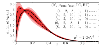
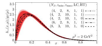
Figure 11: The left and the right panels show the unit-normalized transversity PDFs $h_{-}(x)/g_{T}$ and $h_{+}(x)/g_{T}$ respectively, at $\mu=\sqrt{2}$ MeV as obtained from ${\rm Re}\mathfrak{M}(\nu,z_{3}^{2})$ and ${\rm Im}\mathfrak{M}(\nu,z_{3}^{2})$ using the Jacobi polynomial reconstruction method (see text). The legend specifies the maximum order of Jacobi polynomial used ($N_{J}$), the range of $z_{3}$-values $(z^{\rm min}_{3},z^{\rm max}_{3})$ used, whether the leading higher-twist (HT) correction term was used in the fit (1 or 0), and whether the leading short-distance lattice correction (LC) was used in the fit (1 or 0). The different dashed curves are the central values of the PDFs reconstructed for some samples specifications of $(N_{J},z^{\rm min}_{3},z^{\rm max}_{3},{\rm HT},{\rm LC})$. The inner red band is the 1-$\sigma$ statistical error band and the outer red band is the combined statistical and systematic error (see text).

In Fig. 10, we show the results for $s_{2\pm}^{\rm ans}$ and $s_{4\pm}^{\rm ans}$ from the Jacobi polynomial decomposition of the PDF ansatz based fits. Along with the coefficients $s_{n\pm}$, we have also shown the results for the small-$x$ and large-$x$ exponents $\alpha_{\pm}$ and $\beta_{\pm}$ as inferred from the fits. In each panel, we have shown the estimates for $(\alpha_{\pm},\beta_{\pm},s_{2\pm}^{\rm ans},s_{4\pm}^{\rm ans})$ at different $(z_{3}^{\rm min},z_{3}^{\rm max})$ for the fit ranges. The variability of the fitted parameters with $z_{3}$ range is rather small and within the errors. These values of the exponents were then used to form the family of $P_{n}^{\alpha_{\pm},\beta_{\pm}}$ corresponding to each of the fit ranges. The central values and statistical errors of $s_{n\pm}^{\rm ans}$ for $n$ up to 10 were used as priors and the prior widths in the fits using Eq. (63) as discussed in the step-2 above. It is at once clear from the consistency of $s_{n\pm}$ with zero that the effect of the addition of Jacobi polynomials with $n>0$ on the primary $x^{\alpha_{\pm}}(1-x)^{\beta_{\pm}}$ behavior is rather minimal. This is expected also from the observation that the effect of ${\cal G}=1+\gamma_{\pm}\sqrt{x}+\delta_{\pm}x$, was also minimal, and the transversity PDF could be described to a good accuracy using a simpler $x^{\alpha_{\pm}}(1-x)^{\beta_{\pm}}$ two-parameter ansatz. However, these conclusions are made after the fact and it is important to proceed with the Jacobi basis fits in order to remove the slightest ansatz dependence and estimate the systematic error in a more rigorous manner.

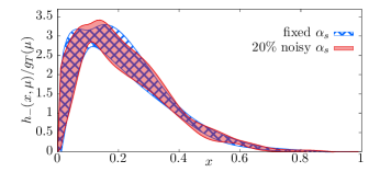
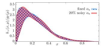
Figure 12: The two panels show the transversity PDFs $h_{\pm}(x)/g_{T}$ reconstructed using $(N_{J}=8,z^{\rm min}_{3}=2a,z^{\rm max}_{3}=8a,{\rm HT=1},{\rm LC=1})$ at a fixed value of the strong-coupling constant $\alpha_{s}(\mu=\sqrt{2}{\ \rm GeV})=0.36$ (shown as the patterned band) are compared with those using the same setup for the fits but $\alpha_{s}(\mu=\sqrt{2}{\ \rm GeV})$ is randomly picked from the normal distribution with the central value of 0.36 and with a width of $20\%$ (shown as the red band).

In Fig. 11, we show the results for $h_{\pm}(x)$ at $\mu=\sqrt{2}$ GeV from the fits using the Jacobi polynomial basis obtained by minimizing the likelihood function ${\cal L}$ in Eq. (66). In the figure, we have shown the central values of $h_{\pm}(x)$ from some representative fitting choices, $\left(N_{J},z_{\rm min},z_{\rm max},{\rm LC},{\rm HT}\right)$. For $h_{-}(x)$, there is less scatter from changes to the fit ranges than for $h_{+}(x)$. For $h_{-}$, there is a tendency for central values with or without the higher-twist term to lie closer together, but such dependences were well within statistical error and taken as part of systematic error. The AIC estimates of the central values and their errors based on Eq. (72) and Eq. (77) are shown as the red bands in the two panels — the darker red inner band includes only the statistical error, whereas the lighter red outer band includes both statistical and systematical errors. The AIC estimators nicely envelope the PDFs resulting from sample individual fit choices. As expected, the systematical error is not negligible in the case of $h_{-}(x)$, whereas the systematic error committed in $h_{+}(x)$ is small compared to the statistical one. The results in Fig. 11 can be seen to be more or less the same as our ansatz based estimation of the transversity PDFs in Fig. 8. From the fits, we can also estimate the Mellin moments. This is useful for making connection with the earlier estimates of $\langle x\rangle_{+}$ obtained via the leading-twist local operator approach, as well as with the possible estimates of $\langle x^{2}\rangle_{-}$ in the future. Focusing on the first two Mellin moments, we find that at $\mu=\sqrt{2}$ GeV,

(78)

$$\frac{\langle x\rangle_{+}}{g_{T}}=0.2285(22)(17);\qquad\frac{\langle x\rangle_{-}}{g_{T}}=0.2199(108)(101),$$ (79)

$$\frac{\langle x^{2}\rangle_{+}}{g_{T}}=0.0787(15)(08);\qquad\frac{\langle x^{2}\rangle_{-}}{g_{T}}=0.0714(27)(12),$$ (80)

(81)

where the errors in the first and second parenthesis are the statistical and systematic errors using the procedure described above. In Refs. Yoon et al. (2017); Mondal et al. (2020a), the values of $g_{T}$ and $\langle x\rangle_{+}$ were computed using the ensembles from the JLab/W&M/LANL collaboration as used in this paper. Unfortunately, the computations in those papers did not include the ensemble used here, and therefore, for the sake of comparison we take the results in Yoon et al. (2017); Mondal et al. (2020a) that have the same lattice spacing $a=0.094$ fm as in this paper, but a slightly lighter pion mass of 270 MeV (which is the ensemble a094m270 as specified in those papers). In these works, the value of tensor charge at 2 GeV scale was found as $g_{T}=0.973(36)$ and $\langle x\rangle_{+}=0.236(11)$, with a systematic variation of about 0.02 around this value . From this, we find their estimate for $\langle x\rangle_{+}/g_{T}=0.242(14)$ at $\mu=2$ GeV (with a systematic variation of about 0.02). In comparison, we find our estimate for $\langle x\rangle_{+}/g_{T}$ to be 5% smaller, which is within a reasonable criteria for tolerance given both the statistical and systematic errors, and the slight mismatch in ${\overline{\mathrm{MS}}}$ renormalization scale $\mu$ in the two studies.

A remaining systematic error is the perturbative uncertainty originating from the transversity matching kernel and the corresponding Wilson coefficients due to the finite perturbative order used. As such, we only know the NLO matching kernel for transversity PDF at this point, and therefore, we do not have a direct way to estimate what the corrections from higher-order terms in the perturbative series would be. This is unlike the unpolarized PDF case, where there are recent results on the two-loop matching Chen et al. (2020b, c); Li et al. (2021), as well as suggestions to estimate the higher-loop uncertainties Gao et al. (2021); Karthik and Sufian (2021). Instead, here we tried to estimate the perturbative uncertainty in a simpler manner through the sensitivity of the results to the value of $\alpha_{s}$ used in the NLO coefficients in Eq. (25) and Eq. (28) — at NLO, the scale $\mu$ at which we need to determine $\alpha_{s}(\mu)$ is not specified and we implicitly assumed $\mu=\sqrt{2}$ GeV, same as the factorization scale of the transversity PDF. Instead of fixing the value of $\alpha_{s}=0.36$ at $\mu=\sqrt{2}$ GeV as done in all the analysis presented above, we tried using a “noisy” $\alpha_{s}$ by randomly sampling $\alpha_{s}\sim{\cal N}(0.36,0.072)$ and use them in the fits. We chose a Gaussian noise width of $20\%$ of $\alpha_{s}=0.36$ as it is approximately the variation resulting in $\alpha_{s}$ by changing the scale from $\mu/2$ to $2\mu$ for $\mu=\sqrt{2}$ GeV, a variation that is traditionally used to evaluate the perturbative uncertainties. The results for $h_{\pm}(x)$ using fixed $\alpha_{s}$ and 20% noisy $\alpha_{s}$ are compared in Fig. 12. We only show a sample case for the fit choice using $N_{J}=8$ Jacobi polynomial reconstruction and $[z_{\rm min},z_{\rm max}]=[2a,8a]$ in the figure, but the comparisons were similar at other choices as well. One can see that the PDF reconstruction is quite robust and only develops slight wiggles when $\alpha_{s}$ is randomly varied, and such variations are masked at the level of precision we are working at. This leads us to think that the perturbative uncertainty of our determination could be mild, and ignore such uncertainties in our final estimate.

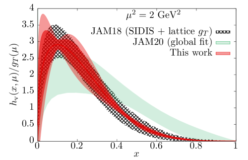
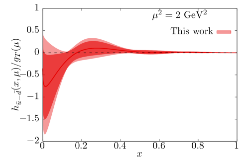
Figure 13: Our lattice determination of the valence transversity distribution $h_{\rm v}(x,\mu)/g_{T}(\mu)$ using the pseudo-distribution approach is shown on the top panel, and the non-singlet antiquark transversity distribution $h_{\bar{u}-\bar{d}}(x,\mu)/g_{T}(\mu)$ is shown on the bottom panel. The factorization scale used is $\mu=\sqrt{2}$ GeV for both the cases. In the two panels, the inner red band includes only the statistical error and the outer red band includes statistical and systematical errors in the PDF reconstruction. For the valence distribution, comparison is made with the previous phenomenological determinations using SIDIS and lattice $g_{T}$ (JAM18) Lin et al. (2018a), shown using a patterned band, and with the recently updated global fit analysis (JAM20) Cammarota et al. (2020) of the single transverse spin asymmetry data (but, without including lattice $g_{T}$), shown as a green band. The non-singlet antiquark distribution is consistent with an isospin symmetric intrinsic sea at all $x$.

In Fig. 13, we present our final estimates of the ${\overline{\mathrm{MS}}}$ transversity PDFs at $\mu=\sqrt{2}$ GeV including the statistical and systematic uncertainties. Our transversity PDF determination is normalized with respect to $g_{T}(\mu)$ at $\mu=\sqrt{2}$ GeV, as in the rest of the paper. In the top panel, we show the valence transversity PDF, $h_{\rm v}(x)=h_{-}(x)$ normalized by $g_{T}(\mu)$. In the bottom panel, we show the non-singlet antiquark distribution given by, $h_{\bar{u}-\bar{d}}(x)=\left[h_{+}(x)-h_{-}(x)\right]/2$ normalized by $g_{T}(\mu)$. The outer red bands in both the panels include both the statistical and systematic errors, whereas the inner red bands include only the statistical error. In the top panel, we have compared our estimate for the valence transversity PDF with the expectations from fits to the experimental data. For this we used two estimates from the Jefferson Angular Momentum Collaboration (JAM) based on two different fitting strategies as well as the processes that were considered. First, we take the result presented in Ref. Lin et al. (2018a) where the analysis was based on fits to the single-transverse spin asymmetry in pion production from deutron and proton targets, and further constrained by the lattice QCD input for the value of $g_{T}$. We refer to this estimate as JAM18 in Fig. 13 and show it as a black patterned band. Second, we take the recent updated result Cammarota et al. (2020) from the JAM collaboration, which considered single-transverse spin asymmetries in pion production via semi-inclusive $e^{+}e^{-}$ annihilation and $pp$ collisions in addition to the SIDIS data, but excluding the lattice input for $g_{T}$. We refer to this estimate as JAM20 in Fig. 13 and show it as the green band. In both cases, we have normalized them to the values of $g_{T}$ in their calculations, namely $g_{T}=1.01(6)$ for JAM18 and $g_{T}=0.86(12)$ for JAM20. While we see an overall agreement of our lattice estimate for the valence transversity PDF with the two phenomenological estimates, the very close agreement of our result with JAM18 result is apparent. The source of the difference Sato between the two phenomenological determinations, JAM18 and JAM20, is likely to arise from the inclusion of single spin asymmetry data from $pp$ collisions from the RHIC experiment that results in a softer approach to zero as $x\to 1$, whereas the SIDIS data alone has a tendency for a harder fall near $x\to 1$. Since the experimental data are not currently very precise to make a distinction between the two behaviors, we expect our lattice determination, that has an inclination towards JAM18 result, could have an impact in the global fit determinations in the near future. However, we need to immediately point the reader to the caveats that unlike the global fit determination of the physical nucleon, our determination is at a heavier-than-physical pion mass and at a fixed lattice spacing. An effect of heavier pion mass could be through the trace terms to the leading-twist OPE which we indirectly accounted for by introducing the nuisance fit terms proportional to $|z_{3}|^{2}$ in our fits and found to be negligible. Another effect could be in changing the intrinsic transversity PDF of the nucleon itself — if this effect is found to be small in the future computations at smaller pion masses, then the overall agreement with the phenomenological determinations would be remarkable. We should also remark that while our lattice estimate could suffer from effects of heavier pion mass, our work is entirely within the collinear framework, whereas the global fits have to include chiral-odd TMD PDFs in order to extract the collinear transversity PDF. In hindsight, the main non-vanishing contributions for $h_{\rm v}(x)$ coming from the intermediate $0.1<x<1$ is perhaps helping the lattice determination due to a reduced small-$x$ uncertainty, unlike for the case of the unpolarized valence PDFs. In the bottom panel of Fig. 13, we find that the non-singlet antiquark transversity PDF, which measures the difference between $\bar{u}$ and $\bar{d}$ in the intrinsic sea of the nucleon, vanishes at all $x$ within the uncertainties — for $x<0.15$, there is a slight excess of $\bar{d}$ compared to $\bar{u}$ if we focus only on the central value, but these effects are statistically insignificant. It should be noted that in the global fit analyses of transversity PDF, a symmetric intrinsic sea is assumed from the start, whereas, our result suggests that the intrinsic sea is indeed symmetric without any such prior assumptions.

VII Conclusions

We presented the formalism for the pseudo-distribution approach to perturbatively match the renormalization group independent ratios to the ${\overline{\mathrm{MS}}}$ transversity PDF. As a consequence, we were able to separate the computation of transversity PDF into two independent computations, namely, one for reconstructing the normalized quantity $h(x)/g_{T}$ using the pseudo-distribution approach, and another for finding $g_{T}$ to set the overall normalization that can be achieved by well-known local operator methods. In this paper, we presented our computation of $h(x)/g_{T}$ and deferred $g_{T}$ to its dedicated computation in the future. We performed our analyses using the nucleon matrix elements for the transversity pseudo-ITD obtained by using the phased distillation approach Egerer et al. (2021a, b), which forms an important novel strategy followed in this paper. We justified the robustness of the excited-state extrapolations required to obtain the matrix elements using the consistency between fits associated with a spectral-decomposition and the summation method. Through an application of the perturbative matching to capture the Ioffe-time dependence at different fixed quark-antiquark separations, $z_{3}$, we showed how to use the lattice data to directly infer the presence of lattice spacing corrections, and to a lesser extent, the higher-twist effects that presumably cancel in the RGI ratio. The above steps formed the back-bone for our reconstruction of the full $x$-dependent normalized transversity PDF $h(x)/g_{T}$ at $\mu=\sqrt{2}$ GeV.

We used parametrized functional forms of $h(x)/g_{T}$ in order to overcome the inverse-problem associated with this approach. First, we reconstructed the transversity distribution by employing a phenomenological functional form of PDFs commonly used in global fits (see Eq. (47)) that is known to describe the cross-sections data over a wide range of $x$ and $Q^{2}$. Using such a reconstructed transversity PDF as our Bayesian prior, we used an expansion of $h(x)/g_{T}$ in terms of a complete basis spanned by Jacobi polynomials Karpie et al. (2021) in order to allow for more flexibility in the PDF reconstruction. This strategy helped us remove any residual model dependence as well as partially answered the question of whether a more complex functional form could in principle change our conclusions. We presented our final results in Fig. 13 for the valence transversity PDF, $h_{\rm v}(x,\mu)/g_{T}$, and for the isovector antiquark transversity PDF, $h_{\bar{u}-\bar{d}}(x,\mu)/g_{T}$. We found a good agreement between our estimate of the valence transversity PDF with the global fit analysis Lin et al. (2018a) based on SIDIS and constraint from lattice $g_{T}$, whereas we found only an overall agreement within larger statistical errors present in the recent global fit analysis of single spin asymmetry data without any lattice input. For the isovector antiquark PDF, which is the difference between the $u$ and $d$ antiquark distributions that are present in the intrinsic sea (that is, not those radiated from the gluons), we found the resulting antiquark asymmetry to be consistent with zero at all values of $x$.

The good agreement between our result for the valence transversity PDF using pseudo-distribution approach is quite encouraging, given comparable statistical errors in our estimate with that obtained in the global fits. Therefore, the lattice computations using perturbative matching approaches are ideal for constraining the transversity PDF in the lack of abundance of DIS cross-section data sensitive to nucleon transversity. The path forward using this approach is quite clear based on the results already presented in this work. The foremost, and also computationally the most challenging, is to extend this computation to finer lattice spacings to reduce the $a/|z_{3}|$ type short-distance lattice correction to DGLAP (seen in Fig. 7); such a correction will always be present at $z_{3}$ of few lattice spacings however small the lattice spacing becomes, but the idea would be to restrict our analysis for physical distance $z_{3}>z_{3}^{\rm min}$ for short-enough $z_{3}^{\rm min}$ so as to ideally not add any corrections to our analysis and rely only on the continuum DGLAP evolution. Second, the good comparison of our estimate in this work with the global-fit result comes with the caveat that our computation was performed at a heavier-than-physical pion mass of 358 MeV. Therefore, it is important to demonstrate that the observation holds as we reduce the pion mass towards the physical point. Based on observations for the unpolarized PDF Joó et al. (2020), one could guess that the effect of pion mass on the intrinsic quark structure of the nucleon is not large. Third, we would like to fold in the estimates of the tensor charge $g_{T}$ directly from the lattice to find $h(x,\mu)$ rather than the ratio $h(x,\mu)/g_{T}$ as in this work. Finally, it would be interesting to use our estimated valence PDF as part of the global fit for transversity PDF, such as those explored in Refs. Bringewatt et al. (2021); Del Debbio et al. (2021); Cichy et al. (2019); Constantinou et al. (2021).

References

- Accardi et al. (2016a) A. Accardi et al., Eur. Phys. J. A 52, 268 (2016a), arXiv:1212.1701 [nucl-ex] .
- Dudek et al. (2012) J. Dudek et al., Eur. Phys. J. A 48, 187 (2012), arXiv:1208.1244 [hep-ex] .
- Chen et al. (2014) J. P. Chen, H. Gao, T. K. Hemmick, Z. E. Meziani, and P. A. Souder (SoLID), (2014), arXiv:1409.7741 [nucl-ex] .
- Harland-Lang et al. (2015) L. A. Harland-Lang, A. D. Martin, P. Motylinski, and R. S. Thorne, Eur. Phys. J. C 75, 204 (2015), arXiv:1412.3989 [hep-ph] .
- Dulat et al. (2016) S. Dulat, T.-J. Hou, J. Gao, M. Guzzi, J. Huston, P. Nadolsky, J. Pumplin, C. Schmidt, D. Stump, and C. P. Yuan, Phys. Rev. D 93, 033006 (2016), arXiv:1506.07443 [hep-ph] .
- Accardi et al. (2016b) A. Accardi, L. T. Brady, W. Melnitchouk, J. F. Owens, and N. Sato, Phys. Rev. D 93, 114017 (2016b), arXiv:1602.03154 [hep-ph] .
- Ball et al. (2017) R. D. Ball et al. (NNPDF), Eur. Phys. J. C 77, 663 (2017), arXiv:1706.00428 [hep-ph] .
- Accardi et al. (2016c) A. Accardi et al., Eur. Phys. J. C 76, 471 (2016c), arXiv:1603.08906 [hep-ph] .
- Ralston and Soper (1979) J. P. Ralston and D. E. Soper, Nucl. Phys. B 152, 109 (1979).
- Artru and Mekhfi (1990) X. Artru and M. Mekhfi, Z. Phys. C 45, 669 (1990).
- Cortes et al. (1992) J. L. Cortes, B. Pire, and J. P. Ralston, Z. Phys. C 55, 409 (1992).
- Jaffe and Ji (1991) R. L. Jaffe and X.-D. Ji, Phys. Rev. Lett. 67, 552 (1991).
- Ji (1992) X.-D. Ji, Phys. Lett. B 284, 137 (1992).
- Anselmino et al. (2007) M. Anselmino, M. Boglione, U. D’Alesio, A. Kotzinian, F. Murgia, A. Prokudin, and C. Turk, Phys. Rev. D 75, 054032 (2007), arXiv:hep-ph/0701006 .
- Airapetian et al. (2005) A. Airapetian et al. (HERMES), Phys. Rev. Lett. 94, 012002 (2005), arXiv:hep-ex/0408013 .
- Ageev et al. (2007) E. S. Ageev et al. (COMPASS), Nucl. Phys. B 765, 31 (2007), arXiv:hep-ex/0610068 .
- Abe et al. (2006) K. Abe et al. (Belle), Phys. Rev. Lett. 96, 232002 (2006), arXiv:hep-ex/0507063 .
- Radici and Bacchetta (2018) M. Radici and A. Bacchetta, Phys. Rev. Lett. 120, 192001 (2018), arXiv:1802.05212 [hep-ph] .
- Bacchetta et al. (2011) A. Bacchetta, A. Courtoy, and M. Radici, Phys. Rev. Lett. 107, 012001 (2011), arXiv:1104.3855 [hep-ph] .
- Benel et al. (2020) J. Benel, A. Courtoy, and R. Ferro-Hernandez, Eur. Phys. J. C 80, 465 (2020), arXiv:1912.03289 [hep-ph] .
- Cammarota et al. (2020) J. Cammarota, L. Gamberg, Z.-B. Kang, J. A. Miller, D. Pitonyak, A. Prokudin, T. C. Rogers, and N. Sato (Jefferson Lab Angular Momentum), Phys. Rev. D 102, 054002 (2020), arXiv:2002.08384 [hep-ph] .
- Ji (2013) X. Ji, Phys. Rev. Lett. 110, 262002 (2013), arXiv:1305.1539 [hep-ph] .
- Ji (2014) X. Ji, Sci. China Phys. Mech. Astron. 57, 1407 (2014), arXiv:1404.6680 [hep-ph] .
- Radyushkin (2017) A. V. Radyushkin, Phys. Rev. D 96, 034025 (2017), arXiv:1705.01488 [hep-ph] .
- Orginos et al. (2017) K. Orginos, A. Radyushkin, J. Karpie, and S. Zafeiropoulos, Phys. Rev. D 96, 094503 (2017), arXiv:1706.05373 [hep-ph] .
- Ma and Qiu (2018a) Y.-Q. Ma and J.-W. Qiu, Phys. Rev. D 98, 074021 (2018a), arXiv:1404.6860 [hep-ph] .
- Ma and Qiu (2018b) Y.-Q. Ma and J.-W. Qiu, Phys. Rev. Lett. 120, 022003 (2018b), arXiv:1709.03018 [hep-ph] .
- Braun and Müller (2008) V. Braun and D. Müller, Eur. Phys. J. C 55, 349 (2008), arXiv:0709.1348 [hep-ph] .
- Sufian et al. (2019) R. S. Sufian, J. Karpie, C. Egerer, K. Orginos, J.-W. Qiu, and D. G. Richards, Phys. Rev. D 99, 074507 (2019), arXiv:1901.03921 [hep-lat] .
- Sufian et al. (2020) R. S. Sufian, C. Egerer, J. Karpie, R. G. Edwards, B. Joó, Y.-Q. Ma, K. Orginos, J.-W. Qiu, and D. G. Richards, Phys. Rev. D 102, 054508 (2020), arXiv:2001.04960 [hep-lat] .
- Martinelli and Sachrajda (1987) G. Martinelli and C. T. Sachrajda, Phys. Lett. B 196, 184 (1987).
- Liu and Dong (1994) K.-F. Liu and S.-J. Dong, Phys. Rev. Lett. 72, 1790 (1994), arXiv:hep-ph/9306299 .
- Chambers et al. (2017) A. J. Chambers, R. Horsley, Y. Nakamura, H. Perlt, P. E. L. Rakow, G. Schierholz, A. Schiller, K. Somfleth, R. D. Young, and J. M. Zanotti, Phys. Rev. Lett. 118, 242001 (2017), arXiv:1703.01153 [hep-lat] .
- Detmold and Lin (2006) W. Detmold and C. J. D. Lin, Phys. Rev. D 73, 014501 (2006), arXiv:hep-lat/0507007 .
- Detmold et al. (2021) W. Detmold, A. V. Grebe, I. Kanamori, C. J. D. Lin, R. J. Perry, and Y. Zhao, (2021), arXiv:2103.09529 [hep-lat] .
- Ji et al. (2021) X. Ji, Y.-S. Liu, Y. Liu, J.-H. Zhang, and Y. Zhao, Rev. Mod. Phys. 93, 035005 (2021), arXiv:2004.03543 [hep-ph] .
- Radyushkin (2020) A. V. Radyushkin, Int. J. Mod. Phys. A 35, 2030002 (2020), arXiv:1912.04244 [hep-ph] .
- Cichy and Constantinou (2019) K. Cichy and M. Constantinou, Adv. High Energy Phys. 2019, 3036904 (2019), arXiv:1811.07248 [hep-lat] .
- Monahan (2018) C. Monahan, PoS LATTICE2018, 018 (2018), arXiv:1811.00678 [hep-lat] .
- Cichy (2021) K. Cichy, in 38th International Symposium on Lattice Field Theory (2021) arXiv:2110.07440 [hep-lat] .
- Egerer et al. (2021a) C. Egerer, R. G. Edwards, C. Kallidonis, K. Orginos, A. V. Radyushkin, D. G. Richards, E. Romero, and S. Zafeiropoulos, (2021a), arXiv:2107.05199 [hep-lat] .
- Karpie et al. (2021) J. Karpie, K. Orginos, A. Radyushkin, and S. Zafeiropoulos, (2021), arXiv:2105.13313 [hep-lat] .
- Joó et al. (2020) B. Joó, J. Karpie, K. Orginos, A. V. Radyushkin, D. G. Richards, and S. Zafeiropoulos, Phys. Rev. Lett. 125, 232003 (2020), arXiv:2004.01687 [hep-lat] .
- Joó et al. (2019) B. Joó, J. Karpie, K. Orginos, A. Radyushkin, D. Richards, and S. Zafeiropoulos, JHEP 12, 081 (2019), arXiv:1908.09771 [hep-lat] .
- Bhat et al. (2021) M. Bhat, K. Cichy, M. Constantinou, and A. Scapellato, Phys. Rev. D 103, 034510 (2021), arXiv:2005.02102 [hep-lat] .
- Fan et al. (2020) Z. Fan, X. Gao, R. Li, H.-W. Lin, N. Karthik, S. Mukherjee, P. Petreczky, S. Syritsyn, Y.-B. Yang, and R. Zhang, Phys. Rev. D 102, 074504 (2020), arXiv:2005.12015 [hep-lat] .
- Alexandrou et al. (2021a) C. Alexandrou, K. Cichy, M. Constantinou, J. R. Green, K. Hadjiyiannakou, K. Jansen, F. Manigrasso, A. Scapellato, and F. Steffens, Phys. Rev. D 103, 094512 (2021a), arXiv:2011.00964 [hep-lat] .
- Alexandrou et al. (2018a) C. Alexandrou, K. Cichy, M. Constantinou, K. Jansen, A. Scapellato, and F. Steffens, Phys. Rev. Lett. 121, 112001 (2018a), arXiv:1803.02685 [hep-lat] .
- Lin et al. (2020) H.-W. Lin, J.-W. Chen, and R. Zhang, (2020), arXiv:2011.14971 [hep-lat] .
- Izubuchi et al. (2019) T. Izubuchi, L. Jin, C. Kallidonis, N. Karthik, S. Mukherjee, P. Petreczky, C. Shugert, and S. Syritsyn, Phys. Rev. D 100, 034516 (2019), arXiv:1905.06349 [hep-lat] .
- Gao et al. (2020) X. Gao, L. Jin, C. Kallidonis, N. Karthik, S. Mukherjee, P. Petreczky, C. Shugert, S. Syritsyn, and Y. Zhao, Phys. Rev. D 102, 094513 (2020), arXiv:2007.06590 [hep-lat] .
- Lin et al. (2021) H.-W. Lin, J.-W. Chen, Z. Fan, J.-H. Zhang, and R. Zhang, Phys. Rev. D 103, 014516 (2021), arXiv:2003.14128 [hep-lat] .
- Alexandrou et al. (2020a) C. Alexandrou, K. Cichy, M. Constantinou, K. Hadjiyiannakou, K. Jansen, A. Scapellato, and F. Steffens, Phys. Rev. Lett. 125, 262001 (2020a), arXiv:2008.10573 [hep-lat] .
- Lin (2020) H.-W. Lin, (2020), arXiv:2008.12474 [hep-ph] .
- Chen et al. (2020a) J.-W. Chen, H.-W. Lin, and J.-H. Zhang, Nucl. Phys. B 952, 114940 (2020a), arXiv:1904.12376 [hep-lat] .
- Khan et al. (2021a) T. Khan et al. (HadStruc), (2021a), arXiv:2107.08960 [hep-lat] .
- Fan et al. (2018) Z.-Y. Fan, Y.-B. Yang, A. Anthony, H.-W. Lin, and K.-F. Liu, Phys. Rev. Lett. 121, 242001 (2018), arXiv:1808.02077 [hep-lat] .
- Fan et al. (2021) Z. Fan, R. Zhang, and H.-W. Lin, Int. J. Mod. Phys. A 36, 2150080 (2021), arXiv:2007.16113 [hep-lat] .
- Fan and Lin (2021) Z. Fan and H.-W. Lin, (2021), arXiv:2104.06372 [hep-lat] .
- Bhattacharya et al. (2016) T. Bhattacharya, V. Cirigliano, S. Cohen, R. Gupta, H.-W. Lin, and B. Yoon, Phys. Rev. D 94, 054508 (2016), arXiv:1606.07049 [hep-lat] .
- Bhattacharya et al. (2015) T. Bhattacharya, V. Cirigliano, S. Cohen, R. Gupta, A. Joseph, H.-W. Lin, and B. Yoon (PNDME), Phys. Rev. D 92, 094511 (2015), arXiv:1506.06411 [hep-lat] .
- Green et al. (2012) J. R. Green, J. W. Negele, A. V. Pochinsky, S. N. Syritsyn, M. Engelhardt, and S. Krieg, Phys. Rev. D 86, 114509 (2012), arXiv:1206.4527 [hep-lat] .
- Aoki et al. (2010) Y. Aoki, T. Blum, H.-W. Lin, S. Ohta, S. Sasaki, R. Tweedie, J. Zanotti, and T. Yamazaki, Phys. Rev. D 82, 014501 (2010), arXiv:1003.3387 [hep-lat] .
- Abdel-Rehim et al. (2015) A. Abdel-Rehim et al., Phys. Rev. D 92, 114513 (2015), [Erratum: Phys.Rev.D 93, 039904 (2016)], arXiv:1507.04936 [hep-lat] .
- Bali et al. (2015) G. S. Bali, S. Collins, B. Glässle, M. Göckeler, J. Najjar, R. H. Rödl, A. Schäfer, R. W. Schiel, W. Söldner, and A. Sternbeck, Phys. Rev. D 91, 054501 (2015), arXiv:1412.7336 [hep-lat] .
- Yamazaki et al. (2008) T. Yamazaki, Y. Aoki, T. Blum, H. W. Lin, M. F. Lin, S. Ohta, S. Sasaki, R. J. Tweedie, and J. M. Zanotti (RBC+UKQCD), Phys. Rev. Lett. 100, 171602 (2008), arXiv:0801.4016 [hep-lat] .
- Mondal et al. (2020a) S. Mondal, R. Gupta, S. Park, B. Yoon, T. Bhattacharya, B. Joó, and F. Winter (Nucleon Matrix Elements (NME)), JHEP 21, 004 (2020a), arXiv:2011.12787 [hep-lat] .
- Mondal et al. (2020b) S. Mondal, R. Gupta, S. Park, B. Yoon, T. Bhattacharya, and H.-W. Lin, Phys. Rev. D 102, 054512 (2020b), arXiv:2005.13779 [hep-lat] .
- Alexandrou et al. (2020b) C. Alexandrou et al., Phys. Rev. D 101, 034519 (2020b), arXiv:1908.10706 [hep-lat] .
- Harris et al. (2019) T. Harris, G. von Hippel, P. Junnarkar, H. B. Meyer, K. Ottnad, J. Wilhelm, H. Wittig, and L. Wrang, Phys. Rev. D 100, 034513 (2019), arXiv:1905.01291 [hep-lat] .
- Bali et al. (2019) G. S. Bali, S. Collins, M. Göckeler, R. Rödl, A. Schäfer, and A. Sternbeck, Phys. Rev. D 100, 014507 (2019), arXiv:1812.08256 [hep-lat] .
- Lin et al. (2018a) H.-W. Lin, W. Melnitchouk, A. Prokudin, N. Sato, and H. Shows, Phys. Rev. Lett. 120, 152502 (2018a), arXiv:1710.09858 [hep-ph] .
- Liu et al. (2018) Y.-S. Liu, J.-W. Chen, L. Jin, R. Li, H.-W. Lin, Y.-B. Yang, J.-H. Zhang, and Y. Zhao, (2018), arXiv:1810.05043 [hep-lat] .
- Alexandrou et al. (2018b) C. Alexandrou, K. Cichy, M. Constantinou, K. Jansen, A. Scapellato, and F. Steffens, Phys. Rev. D 98, 091503 (2018b), arXiv:1807.00232 [hep-lat] .
- Chen et al. (2016) J.-W. Chen, S. D. Cohen, X. Ji, H.-W. Lin, and J.-H. Zhang, Nucl. Phys. B 911, 246 (2016), arXiv:1603.06664 [hep-ph] .
- Alexandrou et al. (2021b) C. Alexandrou, K. Cichy, M. Constantinou, K. Hadjiyiannakou, K. Jansen, A. Scapellato, and F. Steffens, (2021b), arXiv:2108.10789 [hep-lat] .
- Lin et al. (2018b) H.-W. Lin et al., Prog. Part. Nucl. Phys. 100, 107 (2018b), arXiv:1711.07916 [hep-ph] .
- Vogelsang (1998) W. Vogelsang, Phys. Rev. D 57, 1886 (1998), arXiv:hep-ph/9706511 .
- Musch et al. (2011) B. U. Musch, P. Hagler, J. W. Negele, and A. Schafer, Phys. Rev. D 83, 094507 (2011), arXiv:1011.1213 [hep-lat] .
- Ioffe (1969) B. L. Ioffe, Phys. Lett. B 30, 123 (1969).
- Braun et al. (1995) V. Braun, P. Gornicki, and L. Mankiewicz, Phys. Rev. D 51, 6036 (1995), arXiv:hep-ph/9410318 .
- Constantinou and Panagopoulos (2017) M. Constantinou and H. Panagopoulos, Phys. Rev. D 96, 054506 (2017), arXiv:1705.11193 [hep-lat] .
- Ji et al. (2018) X. Ji, J.-H. Zhang, and Y. Zhao, Phys. Rev. Lett. 120, 112001 (2018), arXiv:1706.08962 [hep-ph] .
- Ishikawa et al. (2017) T. Ishikawa, Y.-Q. Ma, J.-W. Qiu, and S. Yoshida, Phys. Rev. D 96, 094019 (2017), arXiv:1707.03107 [hep-ph] .
- Green et al. (2018) J. Green, K. Jansen, and F. Steffens, Phys. Rev. Lett. 121, 022004 (2018), arXiv:1707.07152 [hep-lat] .
- Balitsky and Braun (1989) I. I. Balitsky and V. M. Braun, Nucl. Phys. B 311, 541 (1989).
- Braun et al. (2021) V. M. Braun, Y. Ji, and A. Vladimirov, JHEP 10, 087 (2021), arXiv:2108.03065 [hep-ph] .
- Izubuchi et al. (2018) T. Izubuchi, X. Ji, L. Jin, I. W. Stewart, and Y. Zhao, Phys. Rev. D 98, 056004 (2018), arXiv:1801.03917 [hep-ph] .
- Tanabashi et al. (2018) M. Tanabashi et al. (Particle Data Group), Phys. Rev. D 98, 030001 (2018).
- Edwards et al. (2016) R. Edwards, B. Joó, K. Orginos, D. Richards, and F. Winter, unpublished (2016).
- Yoon et al. (2017) B. Yoon et al., Phys. Rev. D 95, 074508 (2017), arXiv:1611.07452 [hep-lat] .
- Yoon et al. (2016) B. Yoon et al., Phys. Rev. D 93, 114506 (2016), arXiv:1602.07737 [hep-lat] .
- Peardon et al. (2009) M. Peardon, J. Bulava, J. Foley, C. Morningstar, J. Dudek, R. G. Edwards, B. Joo, H.-W. Lin, D. G. Richards, and K. J. Juge (Hadron Spectrum), Phys. Rev. D 80, 054506 (2009), arXiv:0905.2160 [hep-lat] .
- Egerer et al. (2021b) C. Egerer, R. G. Edwards, K. Orginos, and D. G. Richards, Phys. Rev. D 103, 034502 (2021b), arXiv:2009.10691 [hep-lat] .
- Maiani et al. (1987) L. Maiani, G. Martinelli, M. L. Paciello, and B. Taglienti, Nucl. Phys. B 293, 420 (1987).
- Capitani et al. (2012) S. Capitani, M. Della Morte, G. von Hippel, B. Jager, A. Juttner, B. Knippschild, H. B. Meyer, and H. Wittig, Phys. Rev. D 86, 074502 (2012), arXiv:1205.0180 [hep-lat] .
- Khan et al. (2021b) T. Khan, D. Richards, and F. Winter, Phys. Rev. D 104, 034503 (2021b), arXiv:2010.03052 [hep-lat] .
- Karpie et al. (2018) J. Karpie, K. Orginos, and S. Zafeiropoulos, JHEP 11, 178 (2018), arXiv:1807.10933 [hep-lat] .
- Braun et al. (2019) V. M. Braun, A. Vladimirov, and J.-H. Zhang, Phys. Rev. D 99, 014013 (2019), arXiv:1810.00048 [hep-ph] .
- Karpie et al. (2019) J. Karpie, K. Orginos, A. Rothkopf, and S. Zafeiropoulos, JHEP 04, 057 (2019), arXiv:1901.05408 [hep-lat] .
- Golub and Pereyra (1973) G. H. Golub and V. Pereyra, SIAM Journal on Numerical Analysis 10, 413 (1973), https://doi.org/10.1137/0710036 .
- Symonds and Moussalli (2011) M. R. Symonds and A. Moussalli, Behavioral Ecology and Sociobiology 65, 13 (2011).
- Chen et al. (2020b) L.-B. Chen, W. Wang, and R. Zhu, Phys. Rev. D 102, 011503 (2020b), arXiv:2005.13757 [hep-ph] .
- Chen et al. (2020c) L.-B. Chen, W. Wang, and R. Zhu, JHEP 10, 079 (2020c), arXiv:2006.10917 [hep-ph] .
- Li et al. (2021) Z.-Y. Li, Y.-Q. Ma, and J.-W. Qiu, Phys. Rev. Lett. 126, 072001 (2021), arXiv:2006.12370 [hep-ph] .
- Gao et al. (2021) X. Gao, K. Lee, S. Mukherjee, C. Shugert, and Y. Zhao, Phys. Rev. D 103, 094504 (2021), arXiv:2102.01101 [hep-ph] .
- Karthik and Sufian (2021) N. Karthik and R. S. Sufian, Phys. Rev. D 104, 074506 (2021), arXiv:2106.03875 [hep-lat] .
- (108) N. Sato, personal communication .
- Bringewatt et al. (2021) J. Bringewatt, N. Sato, W. Melnitchouk, J.-W. Qiu, F. Steffens, and M. Constantinou, Phys. Rev. D 103, 016003 (2021), arXiv:2010.00548 [hep-ph] .
- Del Debbio et al. (2021) L. Del Debbio, T. Giani, J. Karpie, K. Orginos, A. Radyushkin, and S. Zafeiropoulos, JHEP 02, 138 (2021), arXiv:2010.03996 [hep-ph] .
- Cichy et al. (2019) K. Cichy, L. Del Debbio, and T. Giani, JHEP 10, 137 (2019), arXiv:1907.06037 [hep-ph] .
- Constantinou et al. (2021) M. Constantinou et al., Prog. Part. Nucl. Phys. 121, 103908 (2021), arXiv:2006.08636 [hep-ph] .
- Stanzione et al. (2020) D. Stanzione, J. West, R. T. Evans, T. Minyard, O. Ghattas, and D. K. Panda, in Practice and Experience in Advanced Research Computing, PEARC ’20 (Association for Computing Machinery, New York, NY, USA, 2020) p. 106–111.
- Towns et al. (2014) J. Towns, T. Cockerill, M. Dahan, I. Foster, K. Gaither, A. Grimshaw, V. Hazlewood, S. Lathrop, D. Lifka, G. D. Peterson, R. Roskies, J. Scott, and N. Wilkins-Diehr, Computing in Science & Engineering 16, 62 (2014).
- Edwards and Joo (2005) R. G. Edwards and B. Joo (SciDAC, LHPC, UKQCD), Nucl. Phys. B Proc. Suppl. 140, 832 (2005), arXiv:hep-lat/0409003 .
- Clark et al. (2010) M. A. Clark, R. Babich, K. Barros, R. C. Brower, and C. Rebbi, Comput. Phys. Commun. 181, 1517 (2010), arXiv:0911.3191 [hep-lat] .
- Babich et al. (2010) R. Babich, M. A. Clark, and B. Joo, in SC 10 (Supercomputing 2010) (2010) arXiv:1011.0024 [hep-lat] .
- Winter et al. (2014) F. T. Winter, M. A. Clark, R. G. Edwards, and B. Joó, in 28th IEEE International Parallel and Distributed Processing Symposium (2014) arXiv:1408.5925 [hep-lat] .
- Joó et al. (2013) B. Joó, D. D. Kalamkar, K. Vaidyanathan, M. Smelyanskiy, K. Pamnany, V. W. Lee, P. Dubey, and W. Watson, Lect. Notes Comput. Sci. 7905, 40 (2013).
- Joó et al. (2016) B. Joó, D. D. Kalamkar, T. Kurth, K. Vaidyanathan, and A. Walden, in High Performance Computing, edited by M. Taufer, B. Mohr, and J. M. Kunkel (Springer International Publishing, Cham, 2016) pp. 415–427.