Dynamical Mass of the Young Substellar Companion HD 984 B

Abstract

Model-independent masses of substellar companions are critical tools to validate models of planet and brown dwarf cooling, test their input physics, and determine the formation and evolution of these objects. In this work, we measure the dynamical mass and orbit of the young substellar companion HD 984 B. We obtained new high-contrast imaging of the HD 984 system with Keck/NIRC2 which expands the baseline of relative astrometry from 3 to 8 years. We also present new radial velocities of the host star with the Habitable-Zone Planet Finder spectrograph at the Hobby-Eberly Telescope. Furthermore, HD 984 exhibits a significant proper motion difference between Hipparcos and Gaia EDR3. Our joint orbit fit of the relative astrometry, proper motions, and radial velocities yields a dynamical mass of $61\pm 4$ $\mathrm{M_{Jup}}$ for HD 984 B, placing the companion firmly in the brown dwarf regime. The new fit also reveals a higher eccentricity for the companion ($e=0.76\pm 0.05$) compared to previous orbit fits. Given the broad age constraint for HD 984, this mass is consistent with predictions from evolutionary models. HD 984 B’s dynamical mass places it among a small but growing list of giant planet and brown dwarf companions with direct mass measurements.

1 Introduction

The masses of directly imaged brown dwarfs and giant planets are traditionally inferred from low-temperature cooling models (e.g., Burrows et al. 1997; Saumon & Marley 2008; Phillips et al. 2020). Unlike stars, substellar objects never reach sufficient core temperatures to sustain hydrogen burning. These objects instead lose energy and grow dimmer over their entire lifespans (Kumar, 1963; Burrows et al., 2001). Masses for these objects can then be inferred from their luminosity and age using evolutionary models. These inferred masses are generally uncertain and model-dependent (e.g., Bowler 2016). For instance, the mass of the giant planet 51 Eridani b ranges from $1{-}12$ $\mathrm{M_{Jup}}$ depending on the model choice (Macintosh et al., 2015; Nielsen et al., 2019). Similarly, inferred masses of the wide-separation companion COCONUTS-2b can vary from $\sim 6{-}12$ $\mathrm{M_{Jup}}$ (Zhang et al., 2021).

Several assumptions are made in constructing substellar evolutionary models. A significant parameter, particularly for young objects, is the amount of entropy the planet or brown dwarf starts with immediately post-formation. Objects following hot-start models (e.g., Burrows et al. 1997; Baraffe et al. 2003) begin with arbitrarily large radii and high entropy. Eventually, as hot-start objects cool and contract on a Kelvin-Helmholz timescale, the impact of this initial condition fades. Hot-start grids are thought to better represent formation via gravitational instabilities in a disk or molecular cloud (Spiegel & Burrows, 2012; Chabrier et al., 2014) and are likely to be more applicable to brown dwarf companions than giant planets (e.g, Kratter et al. 2010). Cold-start models strive to more accurately emulate giant planet formation through core accretion by removing initial internal energy (e.g., Marley et al. 2007; Fortney et al. 2008). This reflects the dissipation of energy through accretion shocks and results in much lower luminosities (and thus higher inferred masses of imaged planets) at young ages. Warm-start models (e.g., Spiegel & Burrows 2012; Mordasini 2013; Marleau & Cumming 2014) strike a middle ground between these two classes of models. With intermediate initial entropies, the goal of these models is to portray a more realistic core accretion scenario, with less accretion luminosity lost to radiation than their cold-start counterparts. However, significant uncertainties remain about the initial entropy content of objects that form through these processes. The luminosities of young objects of a given mass and age differ substantially among these three classes of models, resulting in a degeneracy between the inferred mass of a planet or brown dwarf and the formation pathway.

Additional considerations also affect the evolution of substellar objects in these models. The treatment of cloud formation and dissipation can influence giant planet and brown dwarf cooling by modifying their atmospheric opacity. Furthermore, the compositions of atmospheres can impact substellar evolution. This is a subtle effect, however, due to the weak dependence of luminosity on mean opacity (Burrows & Liebert, 1993). Evolutionary models can also differ in the H/He equations of state for modeling high-density matter in brown dwarf and giant planet interiors (e.g., Saumon et al., 1995; Chabrier et al., 2019). As brown dwarfs contract, they reach sufficient temperatures to induce deuterium burning (along with lithium burning for the highest-mass substellar objects; e.g., Gharib-Nezhad et al. 2021). The energy generated during this process is not enough to balance radiative losses, but it results in a slight delay in cooling. The specific details of the onset and eventual cessation of deuterium and lithium burning at a given mass are dependent on metallicity, helium fraction, and initial entropy (Spiegel et al., 2011). This serves as an additional source of variation among brown dwarf cooling models.

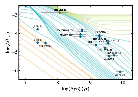
Figure 1: Imaged substellar companions with dynamical masses and bolometric luminosities. Cooling tracks of stars, brown dwarfs, and giant planets from Burrows et al. (1997) are shown in green, blue, and orange, respectively. HD 47127 B (Bowler et al., 2021a) and HD 4113 C (Cheetham et al., 2018) are not included in this plot due to their lack of published bolometric luminosities. The eclipsing brown dwarf binaries 2MASS J05352184-0546085 (Stassun et al., 2006) and 2MASS J15104786-2818174 Aab (Triaud et al., 2020), along with the transiting brown dwarf companion CWW 89Ab (Beatty et al., 2018), have measured dynamical masses but have not been spatially resolved. Unlike most brown dwarfs with dynamical masses, HD 984 B is young and offers an opportunity to assess substellar evolutionary models in an untested region of luminosity-age space near the substellar boundary.

Table 1: Imaged Substellar Companions with Dynamical Masses

Companion	Dynamical Mass	Age	Luminosity	Refs.
	($\mathrm{M_{Jup}}$)	(Myr)	($\log(L_{\mathrm{bol}}/\mathrm{L_{\odot}})$)
$\beta$ Pic c	$8.2\pm 1.0$	$24.0\pm 3.0$	$-4.50\pm 0.04$	1, 2, 3, 4
$\beta$ Pic b	$9.3\pm 2.6$	$24.0\pm 3.0$	$-3.780\pm 0.030$	1, 2, 5
HR 8799 e	$9.6\pm 1.9$	$42\pm 24$	$-4.52\pm 0.10$	6
HD 13724 B	$36.2\pm 1.6$	$2800\pm 500$	$-4.78\pm 0.07$	7
Gl 758 B	$38.0\pm 0.8$	$8300\pm 2700$	$-6.070\pm 0.030$	7, 8
HD 33632 Ab	$50\pm 6$	$1700\pm 400$	$-4.62\pm 0.07$	7
$\mathsf{\varepsilon}$ Indi C	$53.12\pm 0.32$	$\cdots$	$-5.232\pm 0.020$	9, 10
HD 984 B	$61\pm 4$	30–200	$-2.87\pm 0.07$	11, 12, 13
HD 19467 B	$65\pm 6$	$5400\pm 1900$	$-5.19\pm 0.08$	7
HD 4113 C	$66\pm 5$	$5000\pm 1300$	$\cdots$	14
Gl 802 B	$66\pm 5$	${\gtrsim}1000$	$-4.54$	15
HD 4747 B	$66.2\pm 2.5$	$3600\pm 600$	$-4.54\pm 0.06$	16
$\mathsf{\varepsilon}$ Indi B	$68.0\pm 0.9$	$\cdots$	$-4.699\pm 0.017$	9, 10
Gl 229 B	$71.4\pm 0.6$	$3800\pm 1100$	$-5.208\pm 0.007$	7, 17, 18
HD 72946 B	$72.5\pm 1.3$	$1900\pm 600$	$-4.133\pm 0.023$	7
HR 7672 B	$72.7\pm 0.8$	$1920\pm 300$	$-4.19\pm 0.04$	16
Gl 417 C	$99.0\pm 3.0$	300–750	$-4.18\pm 0.04$	19, 20
Gl 417 B	$99.0\pm 3.0$	300–750	$-4.06\pm 0.04$	19, 20
HD 47127 B	$105\pm 18$	7000–10000	$\cdots$	21
HD 130948 C	$114.0\pm 3.0$	400–800	$-3.890\pm 0.030$	19, 20, 22
HD 130948 B	$114.0\pm 3.0$	400–800	$-3.810\pm 0.030$	19, 20, 22

References. — (1) Brandt et al. (2021a); (2) Bell et al. (2015); (3) Nowak et al. (2020); (4) Mathias Nowak, private communication; (5) Morzinski et al. (2015); (6) Brandt et al. (2021b); (7) Brandt et al. (2021c); (8) Bowler et al. (2018); (9) Cardoso (2012); (10) King et al. (2010); (11) This work; (12) Meshkat et al. (2015); (13) Johnson-Groh et al. (2017); (14) Cheetham et al. (2018); (15) Ireland et al. (2008); (16) Brandt et al. (2019); (17) Brandt et al. (2020); (18) Filippazzo et al. (2015); (19) Dupuy et al. (2014); (20) Vigan et al. (2017); (21) Bowler et al. (2021a); (22) Dupuy et al. (2009)

Table 2: Properties of HD 984 A and B

Property	Value	Refs
Host Star
$\alpha_{2000.0}$	00:14:10.25	1
$\delta_{2000.0}$	$-07$:11:56.81	1
$\pi$ (mas)	$21.877\pm 0.025$	1
Distance (pc)	$45.71\pm 0.05$	1
SpT	F7 V	2
Mass ($\mathrm{M_{\odot}}$)	$1.2\pm 0.01$	3, 4, 5
Age (Myr)	$30{-}200$	3
$T_{\mathrm{eff}}$ (K)	6315	6
$\mathrm{[Fe/H]}$ (dex)	${+}0.27$	7
$v\sin i$ ($\mathrm{km/s}$)	$39.3\pm 1.5$	8
$\log(R^{\prime}_{HK})$ (dex)	$-4.34$	9
$\log(L_{X}/L_{\mathrm{bol}})$ (dex)	-4.22	3, 10
RUWE	0.976	1
$B$ (mag)	$7.82\pm 0.02$	11
$V$ (mag)	$7.32\pm 0.01$	11
Gaia $G$ (mag)	$7.2077\pm 0.0028$	1
$J$ (mag)	$6.402\pm 0.023$	12
$H$ (mag)	$6.17\pm 0.04$	12
$K_{s}$ (mag)	$6.073\pm 0.021$	12
Companion
Mass ($\mathrm{M_{Jup}}$)	$61\pm 4$	13
SpT	M$6.5\pm 1.5$	14
$T_{\mathrm{eff}}$ (K)	$2730^{+120}_{-180}$	14
$\log(L_{\mathrm{bol}}/L_{\odot})$ (dex)	$-2.88\pm 0.03$	13
$J$ (mag)	$13.28\pm 0.06$	14
$H$ (mag)	$12.60\pm 0.05$	14
$K_{s}$ (mag)	$12.20\pm 0.04$	13
Semi-Major Axis (AU)	$28^{+7}_{-4}$	13
Eccentricity	$0.76\pm 0.05$	13
Inclination (∘)	$120.8^{+1.8}_{-1.6}$	13
Period (yr)	$140^{+50}_{-30}$	13

References. — (1) Gaia Collaboration et al. (2020); (2) White et al. (2007); (3) Meshkat et al. (2015); (4) Mints & Hekker (2017); (5) Nielsen et al. (2019); (6) Casagrande et al. (2011); (7) Luck (2018); (8) Zúñiga-Fernández et al. (2021); (9) Boro Saikia et al. (2018); (10) Voges et al. (1999); (11) Høg et al. (2000); (12) Skrutskie et al. (2006); (13) This work; (14) Johnson-Groh et al. (2017)

Masses can be directly measured when the dynamical influence that a companion exerts on its host star can be observed. One way to achieve this is to couple observations of the relative motion of the companion with absolute astrometry of the host star. When accompanied by an age constraint and a luminosity measurement, dynamical masses offer a powerful means to empirically calibrate substellar evolutionary models. A comprehensive sample of these benchmark systems across a large dynamic range of age (1 Myr – 10 Gyr) and luminosity ($10^{-7}$ – $10^{-2}$ $L_{\odot}$) would facilitate detailed tests of substellar evolutionary models. These measurements are challenging to obtain, however, due to the long orbital periods of imaged companions. Only 15 dynamical masses have been measured for imaged substellar companions with well-constrained ages (shown in Figure 1 and Table 1). Each new system provides a valuable anchor to empirically map how giant planets and brown dwarfs cool over time.

HD 984 is a young ($30{-}200$ Myr) F7 star with a low-mass companion (Meshkat et al., 2015). Hot-start masses of the companion range from 34 to $94\text{\,}\mathrm{M}_{Jup}$, depending on the adopted system age. HD 984 B is located at a projected separation of ${\sim}200$ mas (${\sim}9.5$ AU), has a contrast of $\Delta H=6.43\pm 0.05$ mag, and a spectral type of M$6.5\pm 1.5$ (Meshkat et al., 2015; Johnson-Groh et al., 2017). Table 1 summarizes the properties of the host star and companion. HD 984 B has been imaged with adaptive optics from $2012{-}2015$ with VLT/NaCo, VLT/SINFONI, and Gemini-S/GPI and shows orbital motion. Additionally, this star exhibits a significant proper motion difference between Hipparcos and Gaia in the Hipparcos-Gaia Catalog of Accelerations (HGCA; Brandt 2018, 2021).

Here, we measure the dynamical mass and 3D orbit of HD 984 B by jointly fitting the HGCA proper motions, relative astrometry, and radial velocities of the system. We obtained new Keck/NIRC2 imaging of the companion to extend the short orbital arc from previous studies as well as new precision radial velocities of the host star with the Habitable-Zone Planet Finder (HPF) spectrograph on the Hobby-Eberly Telescope to measure the radial acceleration of the host star. Section 2 presents our imaging and radial velocity observations. In Section 3, we fit the orbit of HD 984 B, which also constrains the companion’s dynamical mass. In Section 4, we compare our dynamical mass to predicted masses from substellar evolutionary models. Our results are summarized in Section 5.

2 Observations & Data Reduction

2.1 Keck/NIRC2 Adaptive Optics Imaging

We obtained high-contrast imaging of the HD 984 system with the NIRC2 camera at the W.M. Keck Observatory on UT 2019 July 7 and UT 2020 July 30 using natural guide star adaptive optics (Wizinowich, 2013). Our observations consisted of short exposures in $K_{s}$-band with 500 coadded integrations and $t_{\mathrm{int}}=$0.02\text{\,}\mathrm{s}$$ per coadd. We obtained these images without a coronagraph due to the close separation of the companion from its host star (${\sim}200$ mas). To avoid saturating the detector with the unocculted primary, we read out a subarray of $192\times 248$ pixels, which enables shorter integration times. The 2019 and 2020 datasets contained 176 and 120 exposures, respectively. This amounts to 29.3 min and 20 min of total integration time. All images were acquired in pupil-tracking mode to leverage the Angular Differential Imaging (ADI) method (Liu, 2004; Marois et al., 2006). The 2019 and 2020 sequences spanned $30\fdg 5$ and $21\fdg 7$ of sky rotation, respectively.

The first step of our image reduction is subtracting dark frames and flat-fielding the images. Cosmic rays are identified and removed via the L.A.Cosmic algorithm (van Dokkum, 2001). We correct for geometric distortions by applying a piecewise affine transformation to each image using the solution from Service et al. (2016). Frames are then registered by fitting a 2D Gaussian to HD 984, shifted so they are aligned to a common position. We perform this fit twice, which produces superior image alignment over a single iteration or alternatively cross-correlating the frames. Individual images are interpolated with sub-pixel precision using a 3rd-order spline during the alignment process.

We use the Vortex Image Processing (VIP) package (Gomez Gonzalez et al., 2017) to conduct PSF subtraction. VIP offers several choices for PSF subtraction, including non-negative matrix factorization (NMF; Ren et al. 2018), local low-rank plus sparse plus Gaussian-noise decomposition (LLSG; Gomez Gonzalez et al. 2016), and a Principal Component Analysis (PCA) approach similar to the algorithms outlined in Amara & Quanz (2012) and Soummer et al. (2012). We adopt the PCA implementation because of its performance and speed. A lower-dimensional orthogonal basis of eigenimages is first constructed from the full image sequence. The eigenimages (principal components) are found by computing the singular value decomposition of the data cube. The reference PSF is then constructed for a given image by projecting the frame onto this basis. Reference PSFs are subsequently subtracted for each image and the reduced frames are derotated to a common angle and median combined, leaving an image with the signal of the companion added coherently and the residual background predominantly added incoherently.

One advantage of a PCA-based approach is that tuning of the subtraction is largely confined to a single parameter: the number of principal components. Using too few components would undersubtract the host star PSF, while using too many components would subtract more of the companion’s signal. To optimize the number of components, we run the PSF subtraction for each epoch with a total number of components ranging from 1 to 30. We then calculate the signal-to-noise ratio (SNR) for each subtracted image through aperture photometry within a 0.5 FWHM-radius circular aperture. The image coordinates of the companion are determined by fitting a 2D Gaussian to a 14-pixel wide subset of the image around the companion. This is done for each number of principal components. We estimate the noise-level by measuring the flux in non-overlapping apertures at the same angular radius from the star over a range of azimuthal angles excluding that of the companion. A maximum of 24 and 22 non-overlapping noise estimation apertures with radius 0.5 FWHM are used for the 2019 and 2020 epochs, respectively, based on the angular separation of HD 984 B in the images and excluding apertures within 5 aperture radii of the companion. The ratio of the companion flux and the standard deviation of the flux within the noise estimation apertures then yields the SNR. Figure 2 shows the measured SNR for different numbers of components for each epoch. The highest companion SNRs are produced by PSF subtractions of 16 components and 11 components for the 2019 and 2020 epochs, respectively. The subtracted images for each observation are shown in Figure 3.

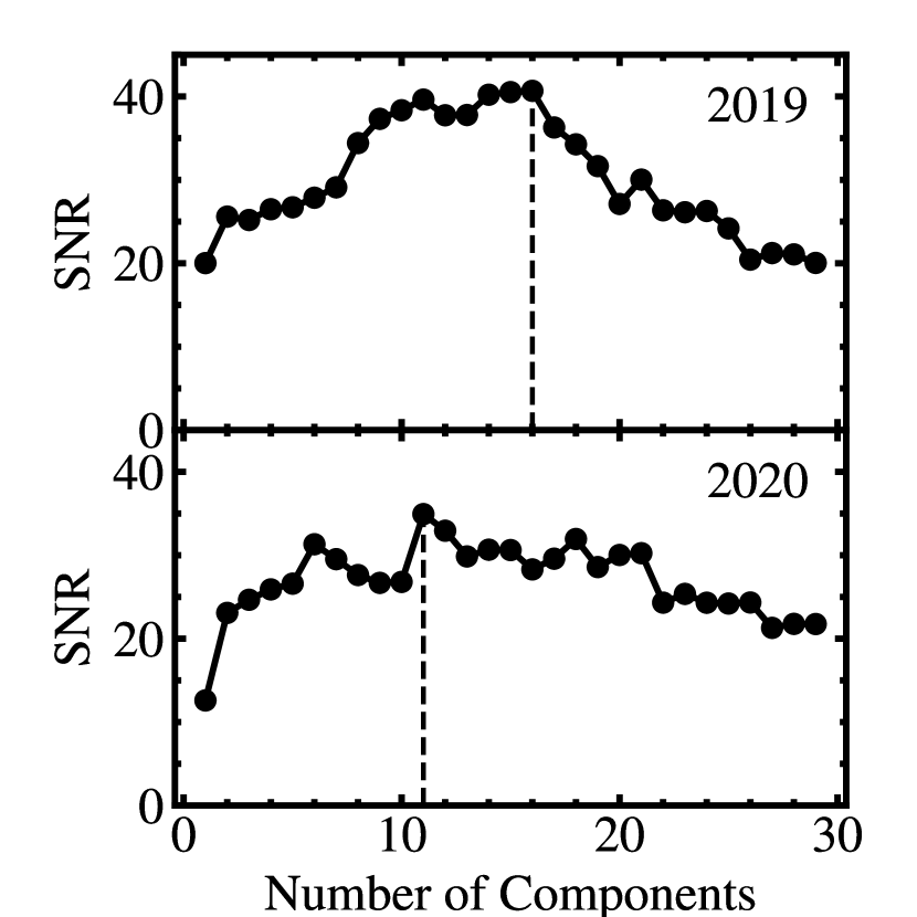
Figure 2: SNR of HD 984 B in PSF-subtracted NIRC2 images as a function of the number of PCA components. We find that a 16-component reduction produces the highest SNR of 40.7 for the 2019 epoch. An 11-component reduction produces the highest SNR of 34.9 for the 2020 epoch. We thus adopt these numbers of components for our PSF subtraction.

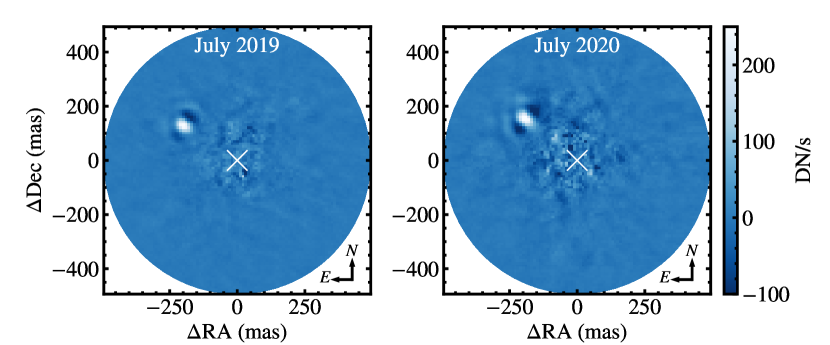
Figure 3: PSF-subtracted images of HD 984 B taken with NIRC2 in July 2019 (left) and July 2020 (right). The color bar corresponds to the flux in each reduced image in units of $\mathrm{DN/s}$. The images are oriented so north is up and east is to the left.

To avoid introducing bias in our astrometry from the PSF subtraction algorithm, we follow the approach of Lagrange et al. (2010) and Marois et al. (2010) of injecting a negative-amplitude PSF template in the original, preprocessed frames at the approximate location of the companion. At the true position of the companion, and with the true flux, the signal of the companion in the final PSF-subtracted image will be removed. For the PSF template, we use the median combination of the images of HD 984 in our ADI sequence. The optimal companion separation ($\rho$), position angle ($\theta$), and flux ratio ($f_{2}/f_{1}$) are measured by minimizing the signal within a circular aperture of 3 FWHM of the PSF template at the location of the companion in the processed image. The companion parameters are first coarsely optimized in the VIP package using the AMOEBA downhill simplex algorithm (Nelder & Mead, 1965). With this as a starting point, the parameter space is then finely explored using the emcee affine-invariant Markov chain Monte Carlo (MCMC) ensemble sampler (Foreman-Mackey et al., 2013). We use 100 walkers to sample our three companion parameters ($\rho$, $\theta$, $f_{2}/f_{1}$) over ${\approx}3\times 10^{4}$ steps. The number of steps is determined by the Gelman-Rubin test for convergence (Gelman & Rubin, 1992). We adopt the default threshold in VIP of $\hat{\mathcal{R}}<1.01$, where $\hat{\mathcal{R}}$ is the Gelman-Rubin statistic which compares the variance between MCMC chains and the variance within individual chains. The flux ratio is then converted to an apparent magnitude of the companion using photometry of HD 984 from 2MASS ($K_{s}=6.073\pm 0.021$ mag; Skrutskie et al. 2006).

Figure 5 shows joint parameter posterior distributions from the MCMC runs for our two epochs. Our new astrometry is listed alongside previous measurements in Table 3. We measure contrasts of $\Delta K_{s}=6.10\pm 0.05$ mag for the 2019 epoch and $\Delta K_{s}=6.15\pm 0.05$ mag for the 2020 epoch. These correspond to apparent magnitudes of HD 984 B of $K_{s}=12.17\pm 0.05$ mag and $K_{s}=12.22\pm 0.05$ mag for each epoch, respectively. These compare well with the previous magnitude measurement from Meshkat et al. (2015) of $K_{s}=12.19\pm 0.04$ mag.

There are four dominant sources of uncertainty for our NIRC2 astrometry: errors in the measurement of the position of the companion, the distortion correction, the plate scale, and north alignment of the detector. Our measurement error is derived from the marginalized MCMC posteriors of the separation $\rho$ and position angle $\theta$. We average the upper and lower error bars of the central $\pm 1\sigma$ (68.3%) confidence interval of each posterior to produce the uncertainties $\sigma_{\mathrm{meas},\rho}$ and $\sigma_{\mathrm{meas},\theta}$. The raw images are corrected for optical distortion effects using the solution from Service et al. (2016). They found that the post-correction residual uncertainties averaged across the detector are about $\sigma_{\mathrm{d}}=$1\text{\,}\mathrm{m}\mathrm{a}\mathrm{s}$$. To convert the astrometry from units of pixels to angular units, we adopt the NIRC2 plate scale from Service et al. (2016). Their plate scale $s$ and associated uncertainty $\sigma_{s}$ are $9.971\pm 0.004\text{\,}\mathrm{m}\mathrm{a}\mathrm{s}\mathrm{/}\mathrm{p}\mathrm{i}\mathrm{x}$. Finally, for the position angle, the Service et al. (2016) distortion correction provides the angle to align the images with celestial north: $\theta_{\mathrm{north}}=0\fdg 262\pm 0\fdg 002$.

The separation in angular units is calculated from the measured separation in units of pixels, $\rho_{\mathrm{meas}}$, via $\rho=s\rho_{\mathrm{meas}}$. The uncertainty on this separation is

$$\sigma_{\rho}=s\rho_{\mathrm{meas}}\bigg{(}\Big{(}\frac{\sigma_{s}}{s}\Big{)}^{2}+\frac{\sigma_{\mathrm{meas},\rho}^{2}+2\sigma_{d}^{2}}{\rho_{\mathrm{meas}}^{2}}\bigg{)}^{1/2}.$$ (1)

The distortion correction uncertainty is multiplied by $\sqrt{2}$ to account for measuring both the position of the host star (during image registration) and the companion (with the negative injection procedure).

The position angle of the companion is found from the uncorrected position angle $\theta_{\mathrm{meas}}$ through

$$\theta=\theta_{\mathrm{meas}}-\theta_{\mathrm{VA}}-\theta_{\mathrm{north}}.$$ (2)

In vertical angle (pupil tracking) mode with NIRC2, $\theta_{\mathrm{VA}}$ is computed from header values in the following manner:

$$\theta_{\mathrm{VA}}=\texttt{PARANG}+\texttt{ROTPOSN}-\texttt{INSTANGL},$$ (3)

where PARANG is the parallactic angle, ROTPOSN is the rotator position, and INSTANGL is the NIRC2 position angle zeropoint of $0\fdg 7$. The uncertainty on the position angle is the error from each term added in quadrature:

$$\sigma_{\theta}=\sqrt{\sigma_{\mathrm{meas},\theta}^{2}+\sigma_{\mathrm{north}}^{2}+\sigma_{d,\theta}^{2}}.$$ (4)

The angular uncertainty from the distortion solution is $\sigma_{d,\theta}\approx\sigma_{d}/\rho$, which is derived by applying the small angle approximation.

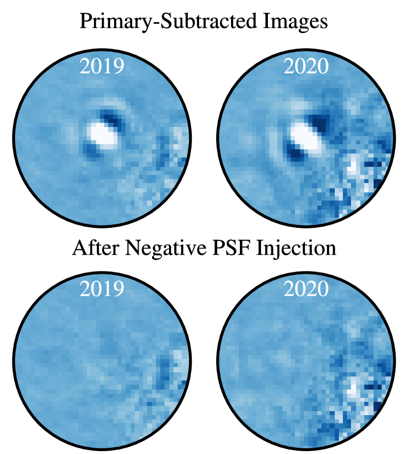
Figure 4: Results of our negative PSF injection. The top panels are the PSF-subtracted images of HD 984 B from our July 2019 and July 2020 NIRC2 datasets. The bottom panels show the results after injecting negative PSF templates with the best-fit separations, position angles, and flux ratios. The elevated noise in the lower-right portion of the images is due to poorer PSF-subtraction closer to the host star.

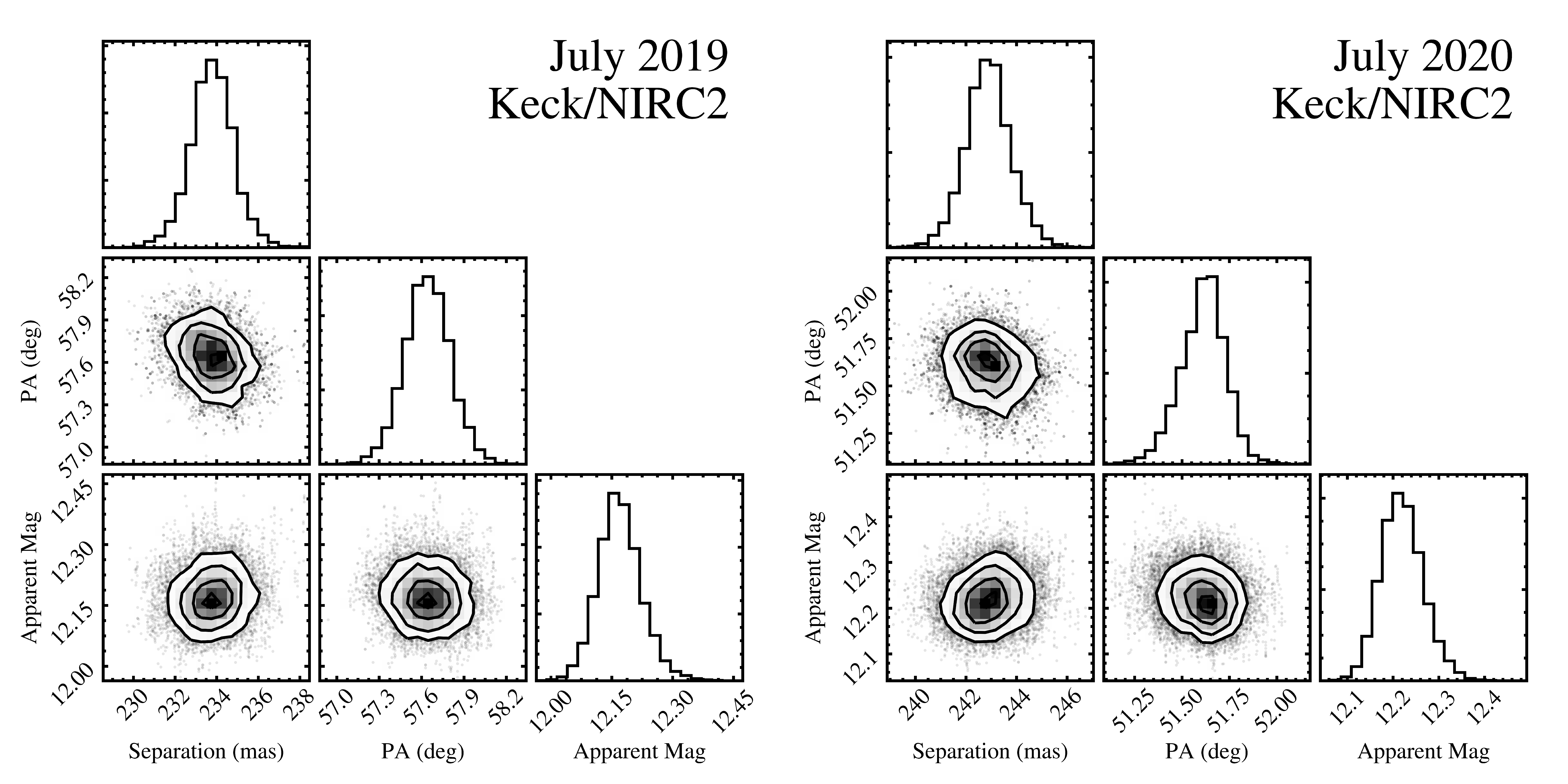
Figure 5: Posterior distributions of HD 984 B astrometry from our July 2019 (left) and July 2020 (right) NIRC2 datasets. The diagonal panels show the marginalized distributions for each parameter. The off-diagonal panels display two-dimensional joint posterior distributions with 1, 2, 3, and $4\sigma$ contours. Astrometry is measured via a negative companion injection approach that uses MCMC to explore the parameter space. All corner plots in this study are produced using corner (Foreman-Mackey, 2016).

Table 3: Relative Astrometry of HD 984 B

Filter	Date	Epoch	Separation	PA	Instrument	Reference
	(UT)	(UT)	(mas)	($\mathrm{\SIUnitSymbolDegree}$)
$L^{\prime}$	2012 Jul 18	2012.545	$190\pm 20$	$108.8\pm 3.0$	NaCo	Meshkat et al. (2015)
$L^{\prime}$	2012 Jul 20	2012.550	$208\pm 23$	$108.9\pm 3.1$	NaCo	Meshkat et al. (2015)
$H+K$	2014 Sep 10	2014.691	$201.6\pm 0.4$	$92.2\pm 0.5$	SINFONI	Meshkat et al. (2015)
$H$	2015 Aug 30	2015.661	$216.3\pm 1.0$	$83.3\pm 0.3$	GPI	Johnson-Groh et al. (2017)
$J$	2015 Aug 30	2015.661	$217.9\pm 0.7$	$83.6\pm 0.2$	GPI	Johnson-Groh et al. (2017)
$K_{s}$	2019 Jul 07	2019.514	$233.8\pm 1.8$	$57.64\pm 0.29$	NIRC2	This Work
$K_{s}$	2020 Jul 30	2020.578	$242.9\pm 1.7$	$51.61\pm 0.26$	NIRC2	This Work

2.2 Radial Velocities

We obtained precision radial velocities of HD 984 with the Habitable-Zone Planet Finder (HPF), a high-resolution ($R\approx 55,000$) near-IR spectrograph on the 9.2-m Hobby-Eberly Telescope (HET) at McDonald Observatory (Mahadevan et al., 2012, 2014). HPF possesses a laser-frequency comb (LFC) calibrator and active temperature stabilization at the milli-Kelvin level (Stefansson et al., 2016) that together enable ${<}$2\text{\,}\mathrm{m}\mathrm{/}\mathrm{s}$$ precision on RV standards (e.g., Metcalf et al. 2019; Tran et al. 2021). The goal of these observations is to measure or constrain the radial component of the acceleration induced by HD 984 B on its host star. Measuring precise RVs of HD 984 is challenging due to its early spectral type (F7), fast rotation ($v\sin{i}=$39.3\pm 1.5\text{\,}\mathrm{k}\mathrm{m}\mathrm{/}\mathrm{s}$$; Zúñiga-Fernández et al. 2021), and young age. Near-IR spectrographs like HPF have been shown to reduce activity-induced jitter by a factor of ${\approx}2-3$ compared to optical spectrographs (Crockett et al., 2012; Gagné et al., 2016; Tran et al., 2021) by sampling wavelengths where starspot-to-photosphere contrasts are reduced.

We obtained a total of 13 RV epochs of HD 984 between UT 2019 September 11 and UT 2020 November 6 (Table 4). Observations were taken in queue mode using the HET’s flexible scheduling system (Shetrone et al., 2007). Each RV epoch of HD 984 consists of three 300-second exposures. For each exposure, 1D spectra are optimally extracted through the standard HPF data-extraction pipeline outlined in Ninan et al. (2018) and Metcalf et al. (2019). Radial velocities are measured using a least-squares matching technique based on the public SERVAL (Zechmeister et al., 2018) package as detailed in Tran et al. (2021). All extracted 1D spectra are first corrected for Earth’s barycentric motion using the barycorrpy (Kanodia & Wright, 2018) software package, and high-frequency pixel-to-pixel variations are removed using a deblazed median master flat spectrum.

All spectra are scaled to the highest SNR spectrum using multiplicative 3rd-order polynomials. This adjusts the spectra to the same flux level on a pixel-to-pixel basis and accounts for variations between observations. The master science template is then created by applying a uniform cubic basic regression to the normalized spectra. The best-fit spline coefficients are calculated by minimizing the residuals between the template and science spectra using a weighted $\chi^{2}$ value. The template undergoes $5\sigma$-clipping to remove points with high residuals; values near the template edge are ignored to account for any edge effects. Telluric absorption and sky emission lines are down-weighted during this process.

The radial velocity shifts and multiplicative polynomials are simultaneously fit by iteratively stepping through a grid of velocities and polynomial coefficients and comparing the template and each science spectrum. The master science template is Doppler shifted in steps of $\Delta v=50$ m s^-1 from $-5$ km s^-1 to 5 km s^-1 and the $\chi^{2}$ residuals are calculated between this shifted template and each science spectrum. During this step, spectral regions in the science spectrum affected by telluric absorption and sky emission lines are masked. The final RV is taken to be the global minimum of the $\chi^{2}-$velocity curve. This process is carried out for 8 spectral orders in the HPF wavelength range least contaminated by telluric absorption. The final RV for a single exposure is the weighted mean of these spectral order RVs, and the standard error is adopted for the final uncertainty. Individual RVs for the contiguous three exposures are then binned together using a weighted mean to produce our RV measurement for a given epoch.

In addition to our HPF radial velocities, we incorporate 21 HARPS RVs in our analysis, which were obtained between UT 2014 July 6 and UT 2016 November 19 (Grandjean et al. 2020; A. Grandjean, private communication). HARPS is a high-resolution ($R\approx 115,000$) optical spectrograph (Mayor et al., 2003) mounted at the 3.6-m ESO telescope at La Silla Observatory. Figure 6 shows our new HPF RVs and the published HARPS RVs. The dispersion of the HPF RVs (48.0 m/s) is lower than that of the HARPS measurements (86.7 m/s) by a factor of 1.8. Nevertheless, the scatter is large in both datasets owing to both the intrinsic activity of HD 984 and the difficulty of measuring precise RVs of F stars, which have fewer spectral features and high rotational velocities compared to later-type stars.

Following Tran et al. (2021), one way to assess the dominant sources of jitter for the two datasets is by considering the metric $\overline{\sigma}/\mathrm{RMS}$, where $\overline{\sigma}$ is the mean measurement uncertainty and $\mathrm{RMS}$ is the root mean square of the RV dataset. If this quantity is small (${<}1.0$), then the jitter is dominated by sources not incorporated into measurement uncertainties, indicating activity as the principal source. If this quantity is larger than 1.0, the RV scatter is captured by the instrumental uncertainties, indicating that spectral features (such as high $v\sin i$ and early spectral type) are the dominant origin of the RV scatter. For the HPF RVs, $\overline{\sigma}/\mathrm{RMS}=1.5$, while for HARPS, $\overline{\sigma}/\mathrm{RMS}=0.2$. This suggests that HD 984’s high $v\sin i$ or broad spectral features are the principal source of jitter for the HPF data, while its spot-induced activity is the dominant source for the HARPS data. This is expected for RVs taken in the near-IR versus the optical.

The presence of an additional close-in stellar or substellar companion could also produce large RV variations on short timescales. We analyzed the HPF and HARPS datasets with a Lomb-Scargle periodogram to identify any periodicity present in the RVs that could correspond to a close-in companion. The periodograms for each instrument do not contain any signals above a false-alarm probability threshold of $0.1\%$.

Another way to assess the presence of close-in, massive companions is with the Renormalised Unit Weight Error (RUWE; Lindegren 2018) statistic in Gaia EDR3, which characterizes the goodness-of-fit for a single-star astrometric solution. RUWE values above ${\sim}1.4$ (and to an extent, above 1; see Stassun & Torres 2021) correlate strongly with the presence of an unresolved binary. HD 984 has an RUWE value of 0.976, indicating that it is well-fit by a single-star solution.

Table 4: HPF Radial Velocities

Date	RV	$\sigma_{\mathrm{RV}}$
($\mathrm{BJD_{TDB}}$)	($\mathrm{m/s}$)	($\mathrm{m/s}$)
$2458737.842$	$-30$	$110$
$2458766.750$	$-10$	$90$
$2458771.741$	$-30$	$50$
$2458819.619$	$-40$	$90$
$2458820.607$	$10$	$3$
$2458821.596$	$-10$	$80$
$2458839.550$	$10$	$60$
$2459063.943$	$140$	$90$
$2459072.917$	$20$	$60$
$2459085.878$	$-45$	$11$
$2459129.754$	$-40$	$40$
$2459145.732$	$10$	$80$
$2459159.664$	$20$	$100$

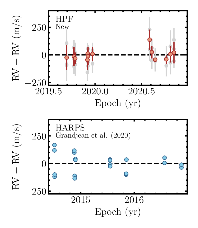
Figure 6: Relative radial velocities of HD 984 from HPF (top panel; this work) and HARPS (bottom panel; Grandjean et al. 2020). HPF RVs from individual exposures are shown in gray, while the final, binned measurements for each visit are shown in red. No clear trends are observed, which may in part be caused by large scatter owing to HD 984’s young age and early spectral type. Nevertheless, their inclusion in the orbit fit places constraints on the radial acceleration induced by HD 984 B.

2.3 Hipparcos-Gaia Acceleration

HD 984 exhibits a significant proper motion difference (astrometric acceleration) between Hipparcos and Gaia which enables the measurement of its dynamical mass. Ensuring that these two astrometric datasets are appropriately cross calibrated is critical for comparing their proper motions. This was recently carried out in the construction of the Hipparcos-Gaia Catalog of Accelerations (HGCA; Brandt 2018). The HGCA provides calibrated proper motions based on corrections of the Hipparcos astrometry to the Gaia frame through local rotations. It also incorporates a $40\%/60\%$ weighting of two Hipparcos reductions (ESA, 1997; van Leeuwen, 2007), inflates uncertainties by fitting an additive error inflation term for Hipparcos and a multiplicative error inflation factor for Gaia, and cross-validates these steps. The result is a robust collection of proper motions with the sensitivity and time baseline (${\sim}25$ years) to enable the measurement of substellar dynamical masses. This has been recently carried out for imaged brown dwarf, giant planet, and white dwarf companions (e.g., Dupuy et al. 2019; Brandt et al. 2019, 2020, 2021a; Currie et al. 2020; Bowler et al. 2021a, b).

Recently, Brandt (2021) updated the HGCA to incorporate proper motions from Gaia EDR3 (Gaia Collaboration et al., 2020). This greatly increases sensitivity to the low-amplitude proper motion changes that substellar companions induce on their host stars. For instance, the significance of the proper motion change for HD 984 increases from $20\sigma$ in the Gaia DR2 version to $62\sigma$ in the Gaia EDR3-equipped HGCA. We use these new cross-calibrated proper motions in the following analysis.

Combining Hipparcos and Gaia astrometry produces three nearly independent proper motions: the individual proper motions at the Hipparcos and Gaia epochs and an average proper motion from the difference in sky position between the two missions. Figure 7 shows these proper motions for HD 984. The measurement derived from the position difference is the most precise, followed by the Gaia EDR3 proper motion. Table 5 lists the absolute HGCA astrometry for HD 984. This star exhibits a tangential acceleration between the Gaia and long-term Hipparcos-Gaia proper motions of $41.6\pm 0.8$ m/s/yr.

Table 5: HGCA Kinematics for HD 984

Parameter	Value
$\mu_{\alpha,\mathrm{Hip}}$ (mas/yr)	$103.4\pm 1.0$
$\mu_{\alpha,\mathrm{Hip}}$ Epoch (yr)	1991.05
$\mu_{\delta,\mathrm{Hip}}$ (mas/yr)	$-66.1\pm 0.5$
$\mu_{\delta,\mathrm{Hip}}$ Epoch (yr)	1991.57
$\mu_{\mathrm{Hip}}$ Correlation Coefficient	0.1119
$\mu_{\alpha,\mathrm{Gaia}}$ (mas/yr)	$104.77\pm 0.05$
$\mu_{\alpha,\mathrm{Gaia}}$ Epoch (yr)	2016.1
$\mu_{\delta,\mathrm{Gaia}}$ (mas/yr)	$-68.016\pm 0.030$
$\mu_{\delta,\mathrm{Gaia}}$ Epoch (yr)	2015.82
$\mu_{\mathrm{Gaia}}$ Correlation Coefficient	0.0384
$\mu_{\alpha,\mathrm{HG}}$ (mas/yr)	$103.326\pm 0.027$
$\mu_{\delta,\mathrm{HG}}$ (mas/yr)	$-66.159\pm 0.018$
$\mu_{\mathrm{HG}}$ Correlation Coefficient	0.269
$\chi^{2}$	3810.4

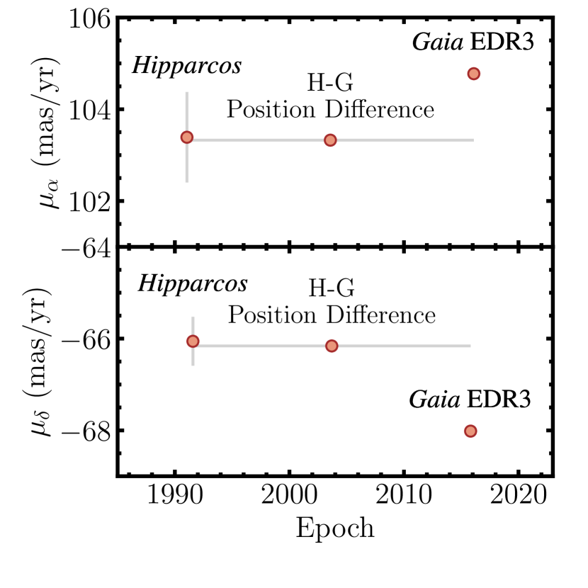
Figure 7: HGCA proper motion measurements of HD 984 in R.A. (top) and Dec. (bottom). Three proper motions are available from the HGCA: the individual Hipparcos and Gaia proper motions and an average proper motion from the difference in sky position between the two missions. For HD 984, the position difference proper motion is the most precise, followed by the Gaia epoch. The slope of these points indicates the time-averaged tangential (sky-plane) acceleration induced by the star’s companion.

3 Orbit Fitting

Our orbit fit incorporates relative astrometry from NaCo, SINFONI, GPI, and NIRC2; radial velocities from HARPS and HPF; and the HGCA proper motions. Astrometry from different instruments and post-processing routines can introduce systematic errors which can bias orbit fits. For example, Bowler et al. (2020) found that the P.A. measurements of the brown dwarf companion DH Tau B had additional scatter not captured by previously reported uncertainties. They attributed this to instrument-to-instrument errors in the distortion correction, north alignment, and/or plate scale. Based on an initial orbit fit of just the relative astrometry with orbitize! (Blunt et al., 2020), we found that the astrometric uncertainties of HD 984 B are likely underestimated: the reduced $\chi^{2}$ value of the best-fit orbit is 5.8. This led us to devise an approach to inflate the uncertainties on the relative astrometry for the subsequent joint orbit fit using all available data.

3.1 Astrometric Error Inflation

Our approach to inflate the astrometric errors is to adopt an astrometric “jitter” term $\sigma_{\mathrm{jit}}$. This term reflects additional positional uncertainty likely resulting from systematics among different instruments. This is added in quadrature to the reported separation uncertainties for our orbit fit:

$$\sigma_{\rho,\mathrm{fit}}=\sqrt{\sigma_{\rho}^{2}+\sigma_{\mathrm{jit}}^{2}}.$$ (5)

The error on the position angle is inflated using this positional jitter term as follows:

$$\sigma_{\theta,\mathrm{fit}}=\sqrt{\sigma_{\theta}^{2}+\bigg{(}\frac{\sigma_{\mathrm{jit}}}{\rho}\bigg{)}^{2}}.$$ (6)

We use orbitize! to find the value of $\sigma_{\mathrm{jit}}$ that produces appropriate error inflation that we would expect for normal standard deviates. orbitize! implements both “Orbits for the Impatient” (OFTI), a Bayesian rejection-sampling approach to orbit fitting detailed in Blunt et al. (2017), and an MCMC approach using the parallel-tempering Markov chain Monte Carlo (PT-MCMC) in emcee (Foreman-Mackey et al., 2013). For the purposes of error inflation, we use the MCMC approach, as it is generally faster for well-constrained orbits. PT-MCMC involves running chains with several different temperatures, where higher-temperature chains more effectively escape local minima and lower-temperature chains more accurately sample peaks in the posterior distribution. Periodically, chains of different temperatures swap positions, enabling the colder ones to be sensitive to additional peaks present in the posterior accessed by higher-temperature chains. This approach is better suited to sampling the complex multi-model posteriors that can arise when fitting orbits. We used a total of 20 temperatures for each orbit fit, adopting the coldest set of chains for the posterior distribution. We experimented with different numbers of steps and found that a total of $10^{5}$ steps over $100$ walkers sampled the parameter space well. We discard the first $50\%$ of each chain as burn-in.

For each jitter value, we compute the reduced Chi-squared value $\chi^{2}_{\nu}$ through

$$\chi^{2}_{\nu}=\frac{1}{\nu}\bigg{(}\sum_{i}\frac{(\rho_{i}-M_{\rho,i})^{2}}{\sigma_{\rho,\mathrm{fit},i}^{2}}+\sum_{i}\frac{(\theta_{i}-M_{\theta,i})^{2}}{\sigma_{\theta,\mathrm{fit},i}^{2}}\bigg{)},$$ (7)

where $\nu$ is the number of degrees of freedom; $\rho_{i}$ and $\theta_{i}$ are the separation and position angle measurement, respectively; and $M_{\rho,i}$ and $M_{\theta,i}$ are the corresponding model values for the separation and position angle. The maximum likelihood orbit is used for the model to compute $\chi^{2}_{\nu}$. The number of degrees of freedom is the difference between the number of datapoints (16; seven measurements of the separation and position angle, plus the parallax and system mass) and the eight fitted parameters.

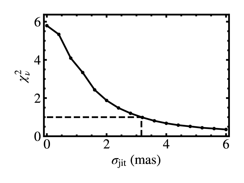
Figure 8: Reduced $\chi^{2}$ values from orbit fits to the ensemble of relative astrometry for HD 984 as a function of increasing astrometric jitter. An astrometric jitter of $\sigma_{\mathrm{jit}}=$3.17\text{\,}\mathrm{m}\mathrm{a}\mathrm{s}$$ yields $\chi^{2}_{\mathrm{\nu}}=1.0$. We therefore inflate the relative astrometry uncertainties by this amount for the final joint orbit fit.

Figure 8 shows the result of this procedure. Through 3rd-order spline interpolation, we find that an astrometric jitter value of $\sigma_{\mathrm{jit}}=$3.17\text{\,}\mathrm{m}\mathrm{a}\mathrm{s}$$ produces $\chi_{\nu}^{2}=1.0$. We adopt this value for the full orbit fit, using Equations 5 and 6 to inflate the raw separation and position angle measurements, respectively.

Table 6: HD 984 B Orbit Fit Results

Parameter	Median $\pm 1\sigma$	95.4% C.I.	Prior
Fitted Parameters
$M_{\mathrm{comp}}$ $(\mathrm{M_{Jup}})$	$61\pm 4$	(53, 69)	$1/M_{\mathrm{comp}}$ (log-flat)
$M_{\mathrm{host}}$ $(\mathrm{M_{\odot}})$	$1.16\pm 0.10$	(0.94, 1.36)	$1.2\pm 0.1\text{\,}\mathrm{M}_{\odot}$ (Gaussian)
$a$ $(\mathrm{AU})$	${28}_{-4}^{+7}$	(21, 46)	$1/a$ (log-flat)
$i$ $($\mathrm{\SIUnitSymbolDegree}$)$	${120.8}_{-1.6}^{+1.8}$	(117.6, 124.8)	$\sin(i)$, $$0\text{\,}\mathrm{\SIUnitSymbolDegree}$<i<$180\text{\,}\mathrm{\SIUnitSymbolDegree}$$
$\sqrt{e}\sin{\omega}$	${-0.62}_{-0.03}^{+0.07}$	(-0.68, 0.64)	Uniform
$\sqrt{e}\cos{\omega}$	${0.59}_{-0.08}^{+0.06}$	(-0.68, 0.72)	Uniform
$\Omega$ $($\mathrm{\SIUnitSymbolDegree}$)$	${115}_{-7}^{+10}$	(101, 303)	Uniform
$\lambda_{\mathrm{ref}}$ $($\mathrm{\SIUnitSymbolDegree}$)$	${312}_{-7}^{+6}$	(130, 324)	Uniform
$\bar{\omega}$ $($\mathrm{m}\mathrm{a}\mathrm{s}$)$	$21.877\pm 0.004$	(21.868, 21.885)	$21.877\pm 0.025\text{\,}\mathrm{m}\mathrm{a}\mathrm{s}$ (Gaussian)
HPF RV Jitter $\sigma_{\mathrm{HPF}}$ $\mathrm{(m/s)}$	${0}_{-0}^{+26}$	(0, 49)	$1/\sigma_{\mathrm{HPF}}$ (log-flat), $\sigma_{\mathrm{HPF}}\in[0,1000$\mathrm{m}\mathrm{/}\mathrm{s}$]$
HARPS RV Jitter $\sigma_{\mathrm{HARPS}}$ $\mathrm{(m/s)}$	${89}_{-13}^{+17}$	(66, 130)	$1/\sigma_{\mathrm{HARPS}}$ (log-flat), $\sigma_{\mathrm{HARPS}}\in[0,1000$\mathrm{m}\mathrm{/}\mathrm{s}$]$
Derived Parameters
$P$ (yr)	${140}_{-30}^{+50}$	(90, 280)	. . .
$e$	$0.76\pm 0.05$	(0.64, 0.85)	. . .
$\omega$ $($\mathrm{\SIUnitSymbolDegree}$)$	${314}_{-3}^{+4}$	(308, 323)	. . .
$T_{0}$ $(\mathrm{JD})$	${2461600}_{-1700}^{+2500}$	(2457600, 2468400)	. . .
$q$ $(=M_{\mathrm{comp}}/M_{\mathrm{host}})$	${0.0500}_{-0.0023}^{+0.0029}$	(0.0458, 0.0571)	. . .

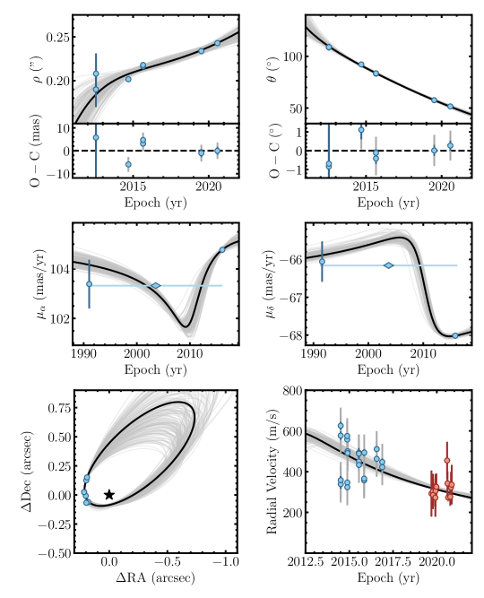
Figure 9: Orbit fit of HD 984 B compared to the relative astrometry (top panels), HGCA acceleration of its host star (middle panels), sky-projected orbit (bottom left), and radial velocities (bottom right). The gray curves show 150 randomly drawn orbits from the MCMC chains. The maximum-likelihood orbit is highlighted in black. In the RV plot, the red points are HPF RVs, while the blue points are HARPS RVs. The gray error bars in the relative astrometry plots are the inflated uncertainties, while the blue error bars are the original uncertainties. The gray error bars in the RV plot incorporate the jitter terms from the best-fit orbit ($\sigma_{\mathrm{HARPS}}$ and $\sigma_{\mathrm{HPF}}$), while the blue and red error bars are the original instrumental uncertainties.

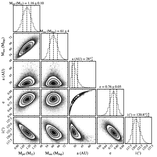
Figure 10: Joint posterior distributions for select parameters in the orbit fit of HD 984 B. Diagonal panels show the marginalized posteriors for each parameter. The dynamical mass of HD 984 B is $61\pm 4$ $\mathrm{M_{Jup}}$, placing the companion firmly in the brown dwarf regime.

3.2 3D Orbit

The mass and orbit of HD 984 B are determined by jointly fitting the relative astrometry, radial velocities, and proper motion difference between Hipparcos and Gaia using the orvara package (Brandt et al., 2021d). orvara implements an efficient method of solving Kepler’s equation based on the approach described in Raposo-Pulido & Peláez (2017). This yields absolute errors below $2\times 10^{-14}$ for $e<0.9999$.

The orbital parameter posteriors are sampled via the parallel-tempering Markov chain Monte Carlo (PT-MCMC) ensemble sampler in emcee (Foreman-Mackey et al., 2013). The following eight quantities define a Keplerian orbit: semimajor axis ($a$), inclination ($i$), longitude of ascending node ($\Omega$), time of periastron passage ($T_{0}$), eccentricity ($e$), argument of periastron ($\omega$), and the masses of the two components ($M_{\mathrm{host}}$ and $M_{\mathrm{comp}}$). Eccentricity and argument of periastron are fit as $\sqrt{e}\sin\omega$ and $\sqrt{e}\cos\omega$, which avoids the Lucy-Sweeny bias against circular orbits (Lucy & Sweeney, 1971). orvara fits a single RV jitter term $\sigma_{\mathrm{jit}}$ to capture RV variations caused by activity that are not reflected in the instrumental uncertainties. The HARPS RVs of HD 984 have a higher scatter than the HPF RVs while also having lower measurement uncertainties, so we modified orvara to fit two RV jitter terms for each instrument, $\sigma_{\mathrm{HARPS}}$ and $\sigma_{\mathrm{HPF}}$. The package analytically marginalizes over the barycenter proper motion, the RV zero points for the HARPS and HPF datasets ($\mathrm{RV}_{\mathrm{zero}}$), and the parallax. Like the orbitize! fits, we used PT-MCMC to fit a total of 20 temperatures, where the coldest set of chains describes the posterior distributions. We found that 100 walkers over $10^{6}$ steps samples the parameter space well. We discard the first 250,000 steps as burn-in.

Our priors and orbit fit results are listed in Table 6. We adopt a prior on the host star mass of $1.2\pm 0.1\text{\,}\mathrm{M}_{\odot}$, which encompasses typical mass estimates for HD 984 in the literature (e.g., $1.2\pm 0.06\text{\,}\mathrm{M}_{\odot}$ from Meshkat et al. 2015; $1.15\pm 0.06\text{\,}\mathrm{M}_{\odot}$ from Mints & Hekker 2017; $1.28\text{\,}\mathrm{M}_{\odot}$ from Nielsen et al. 2019). For the prior on the parallax, we adopt the Gaia EDR3 value of $21.877\pm 0.025\text{\,}\mathrm{m}\mathrm{a}\mathrm{s}$. All other priors are uninformative and can be found in Table 6.

Figure 9 overplots the relative astrometry, absolute Hipparcos-Gaia astrometry, radial velocities, and sky-projected relative offsets on a sample of the orbit solutions. The maximum-likelihood orbit is highlighted in black. Our new relative astrometry in 2019 and 2020 significantly extends the previous orbital arc, resulting in a shallower slope in separation than previous orbit fits that only incorporated the 2012–2015 astrometry (see panel (a) of Figure 13 from Bowler et al. 2020). Note that the middle measurement in the Hipparcos-Gaia data is an average proper motion based on scaled positions in HGCA and reflects the astrometric reflex motion over the entire 25-year time baseline between the two missions. For clarity, we only show orbits in the RV plot with $\omega>$226\text{\,}\mathrm{\SIUnitSymbolDegree}$$. There are two distinct clusters of orbits with arguments of periastra $180\text{\,}\mathrm{\SIUnitSymbolDegree}$ apart that correspond to the star approaching and receding Earth at the time our observations were taken. This is due to the RV datasets lacking the time baseline or RV precision to unambiguously constrain the direction of the radial acceleration.

Joint posteriors of host star mass, companion mass, and select orbital elements are shown in Figure 10. The dynamical mass of HD 984 B is $61\pm 4$ $\mathrm{M_{Jup}}$, which places it firmly in the brown dwarf regime (${\lesssim}$75\text{\,}\mathrm{M}_{Jup}$$) at 99.7% significance. The inclination of $i=120\fdg 8^{+1.8}_{-1.6}$ from our fit is consistent with the previous measurement of $i=120^{+6.1}_{-7.3}{}^{\circ}$ in Bowler et al. (2020), while the semi-major axis increases from $a=17.6^{+4.3}_{-8.1}$ AU from Bowler et al. (2020) to $a=28^{+7}_{-4}$ AU. The eccentricity increases substantially between the orbit fits: the previous fit found $e=0.23^{+0.11}_{-0.23}$, while our new orbit fit yields an eccentricity of $e=0.76\pm 0.05$. The difference in $a$ and $e$ can largely be attributed to the increased orbit coverage and astrometric acceleration we make use of in this fit. The higher eccentricity is consistent with the primary conclusion of Bowler et al. (2020) that brown dwarf companions exhibit a broad eccentricity distribution. This stands in contrast to imaged planets which preferentially have low eccentricities.

Among the relative astrometry datasets, the 2014 SINFONI data largely drives the error inflation. Compared to the other separation measurements, it has the smallest uncertainty by a factor of ${\sim}2$. Excluding the SINFONI astrometry from the orbitize! fit of the isolated relative astrometry produces $\chi^{2}_{\nu}=1.1$. To ensure that the inclusion of this point is not significantly influencing the final orbit fit, we performed an additional orvara fit omitting the SINFONI astrometry, which yields $M_{\mathrm{comp}}=61\pm 4$ $\mathrm{M_{Jup}}$, $a=29^{+5}_{-3}$ AU, $e=0.75\pm 0.03$, and $i=119\fdg 8\pm 1\fdg 7$. These results are consistent with the orbit fit that includes all astrometry with inflated uncertainties.

The time of periastron for our orbit fit (in calendar years) of $T_{0}={2028}_{-5}^{+7}$ is close to the epoch of our relative astrometry (2012–2020), especially in comparison to the orbital period of $P={140}_{-30}^{+50}$ yr. From Kepler’s second law, eccentric companions spend a significantly smaller fraction of time near periastron compared to apastron. Finding that an eccentric companion happened to be discovered near periastron could be a sign that systematic errors are present in the astrometry. While the companion could of course be in that position in its orbit, another possibility is that this is caused by underestimated errors in the astrometry. Additional systematics not captured in the error inflation would produce larger velocity changes between observations, causing the orbit fit to prefer eccentric solutions with periastron near the epoch of the astrometry. Another explanation is that eccentric companions near periastron produce the most precise orbits over short orbital arcs, causing a selection effect that favors companions with these types of orbits, as they are most amenable to precise dynamical mass measurements. Further monitoring of this system will determine whether HD 984 B is truly near periastron.

4 Discussion

4.1 Age of HD 984

Determining the age of the HD 984 system has proven to be challenging. The spectral type (F7) and effective temperature $T_{\mathrm{eff}}=$6315\text{\,}\mathrm{K}$$ (Casagrande et al., 2011) of HD 984 place it at the Kraft break (Kraft, 1967), which separates lower-mass stars with deep convective envelopes and higher-mass stars with thin convective envelopes. Convective zones play important roles in generating magnetic winds that drive angular momentum loss. Stars with masses above the Kraft break tend to retain their initial rotation rates, while stars below that threshold spin down over their lifespans. This leads to the breakdown of standard gyrochronological relations such as Mamajek & Hillenbrand (2008) for stars like HD 984. It also hampers activity-based age indicators, as activity is caused by a star’s magnetic dynamo. For instance, BAFFLES (Stanford-Moore et al., 2020) returns a broad age posterior with a median value of $444\text{\,}\mathrm{M}\mathrm{y}\mathrm{r}$ and 95% confidence interval of 57–6670 Myr for the $\log(R^{\prime}_{HK})=-4.34$ dex measurement from Boro Saikia et al. (2018).

Meshkat et al. (2015) carried out a detailed age analysis of HD 984 and settled on a range of $30-200$ Myr. The low end is derived from isochronal fitting, which produces a broad age distribution with a lower limit of ${\sim}$30\text{\,}\mathrm{M}\mathrm{y}\mathrm{r}$$ set by the time that it takes for $1.2\text{\,}\mathrm{M}_{\odot}$ stars to settle onto the zero-age main sequence. The upper limit is inferred from HD 984’s X-ray luminosity ($\log(L_{X}/L_{\mathrm{bol}})=$-4.22\text{\,}\mathrm{d}\mathrm{e}\mathrm{x}$$; Voges et al. 1999; Meshkat et al. 2015), Ca II H&K emission (Meshkat et al. 2015 adopted a mean value of $\log(R^{\prime}_{HK})\approx-4.40$ dex), and projected rotational velocity ($v\sin i=42.13\pm 1.65$ km/s; White et al. 2007). To overcome the challenges produced by the star’s position at the Kraft break, Meshkat et al. (2015) compare these quantities against a sample of nearby stars with the same spectral type and find that HD 984 is among the youngest $1{-}5$ percent of field F7 dwarfs. This sets an upper limit on the age of HD 984 of ${\sim}200$ Myr based on the main-sequence lifetime of 1.2 $\mathrm{M_{\odot}}$ stars of ${\sim}5000$ Myr.

HD 984 was observed by TESS (Ricker et al., 2014) in Sector 3 (TIC 408012706), which presents the possibility of refining its age through gyrochronology or asteroseismology. Its light curve exhibits significant periodicity indicative of rotation. Analyzing the lightcurve with a Lomb-Scargle periodogram and fitting a Gaussian to the highest peak to estimate the uncertainty yields a rotation period of $1.381\pm 0.012$ d. The Mamajek & Hillenbrand (2008) relations with $B-V=0.500\pm 0.022$ mag (Høg et al., 2000) imply an age of $200$ Myr with a $1\sigma$ upper limit of 700 Myr, where the large uncertainty is due to HD 984’s position near the Kraft break. Note that the minimum value of $B-V$ for which the Mamajek & Hillenbrand (2008) relations are valid is $B-V=0.5$ mag—exactly matching that for HD 984. Asteroseismology offers another possible avenue to determine the age of HD 984. We smoothed and subtracted the TESS light curve with a box filter to remove large periodic structure from stellar rotation and examined the residuals. A Lomb-Scargle periodogram of the residuals shows no significant peaks, so the potential to revise the age of HD 984 via asteroseismology is limited with the current precision from TESS.

Zuckerman et al. (2011) considered HD 984 to be a member of the $42^{+6}_{-4}$ Myr Columba young association primarily on the basis of its $UVW$ kinematics derived from Hipparcos astrometry (Torres et al., 2008; Bell et al., 2015). Newer Gaia EDR3 astrometry and the Gaia DR2 radial velocity produce $UVW$ space motions of $U=-12.47\pm 0.03$ km/s, $V=-22.37\pm 0.19$ km/s, and $W=-8.8\pm 0.5$ km/s. Compared with the mean velocities of Columba from Gagné et al. (2018) of $(UVW)=(-11.9\pm 1.0,-21.3\pm 1.3,-5.7\pm 0.7)$ km/s, HD 984 is discrepant primarily in its $W$ velocity by $3.6\sigma$, or $3.1\pm 0.9$ km/s. BANYAN $\Sigma$ (Gagné et al., 2018) yields a $99.6\%$ probability that HD 984 is a field star based on its Gaia EDR3 astrometry and Gaia DR2 radial velocity. However, BANYAN $\Sigma$ is susceptible to membership misassignments or omissions as a result of assumptions about cluster spatial and kinematic structure (e.g., Bowler et al. 2017; Desrochers et al. 2018), so HD 984 could potentially still be a member of the association. We used FriendFinder to search for potential co-moving neighbors (either distantly bound or as a cluster) of HD 984 that could help age-date the system (e.g., Tofflemire et al. 2021). This tool queries the Gaia EDR3 source catalog for apparent comoving stars within a $25\text{\,}\mathrm{p}\mathrm{c}$ volume that have a tangential (sky-plane) velocity offset from HD 984 B’s proper motion of ${<}$5\text{\,}\mathrm{k}\mathrm{m}\mathrm{/}\mathrm{s}$$. No overdensity of stars above the main sequence consistent with membership in a young moving group is apparent. Based on the lack of a convincing kinematic match to Columba or other young comoving stars, we adopt the age estimate of 30–200 Myr from Meshkat et al. (2015) for HD 984 A and B.

4.2 Bolometric Luminosity of HD 984 B

We calculate the bolometric luminosity of HD 984 B via the $M_{H,\mathrm{2MASS}}-\log(L_{\mathrm{bol}}/L_{\odot})$ relation from Dupuy & Liu (2017). We first convert the $H$-band magnitude of the companion from the MKO photometric system to the 2MASS photometric system using the empirical $H_{\mathrm{MKO}}-H_{\mathrm{2MASS}}$ formula from Dupuy & Liu (2017). Converting to an absolute magnitude using the Gaia EDR3 parallax yields $M_{H,2MASS}=9.27\pm 0.05$ mag, which corresponds to a bolometric luminosity of $\log(L_{\mathrm{bol}}/L_{\odot})=-2.88\pm 0.03$ dex. Although the Dupuy & Liu (2017) luminosity relation is based on dynamical masses of field objects, bolometric corrections for field and young ultracool dwarfs agree for mid- and late-M dwarfs (Filippazzo et al., 2015). Our value agrees with both the luminosity that Johnson-Groh et al. (2017) determined by fitting DUSTY models (Chabrier et al., 2000) to $J$- and $H$-band photometry of the companion ($-2.88\pm 0.07$ dex) and the value from Meshkat et al. (2015) who applied M6.5 dwarf bolometric corrections to NaCo and SINFONI photometry ($-2.815\pm 0.024$ dex). We adopt our revised value for this analysis.

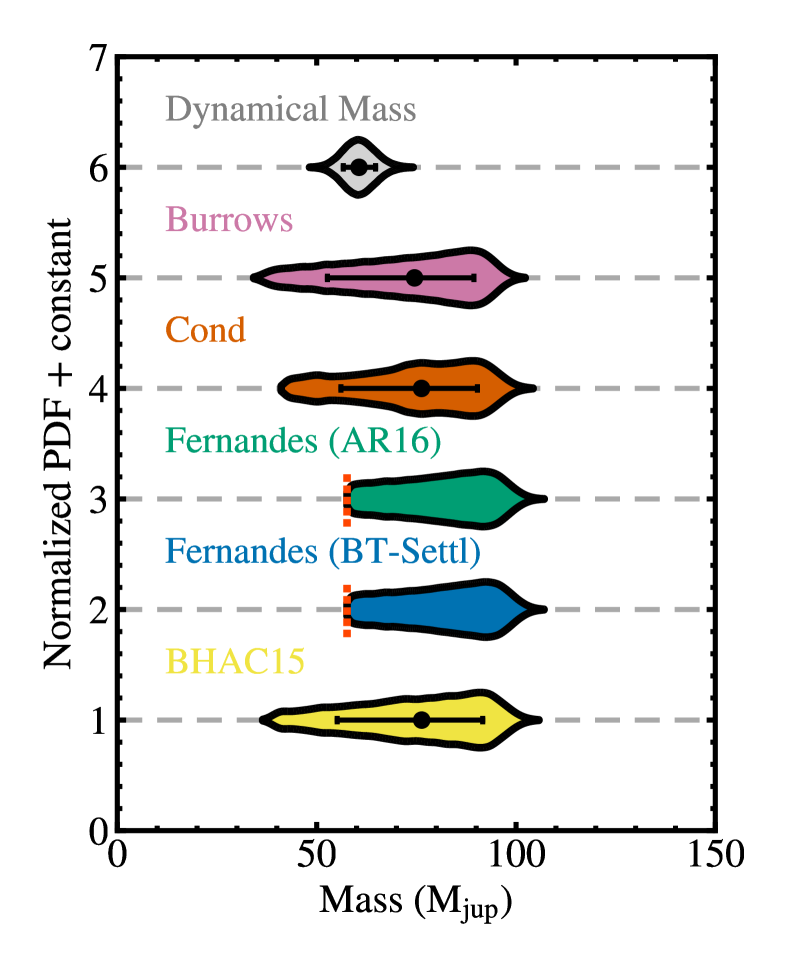
Figure 11: Dynamical mass of HD 984 B (top distribution) compared to inferred mass distributions for a variety of hot-start evolutionary models. Mass distributions are assembled for a given model by sampling the luminosity and age distributions of HD 984 B $10^{6}$ times, and then linearly interpolating the model grid to produce a corresponding mass for each trial. For the Fernandes et al. (2019) models, the predicted mass distributions are limited to ${>}$57.6\text{\,}\mathrm{M}_{Jup}$$, which is the lowest-mass track computed in their study (see Figure 13). These inferred masses are thus overestimates of the true model predictions for these two grids. The median and 68.3% confidence interval are shown for each complete distribution. Each model prediction is broadly consistent with our measured dynamical mass.

4.3 Model Comparison

Our dynamical mass measurement of HD 984 B can be directly compared with the predicted masses of substellar evolutionary models. A variety of publicly available hot-start evolutionary models are selected for this comparison based on the luminosity and age of HD 984 B. Specifically, we generate inferred mass distributions from the pre-computed grids of Burrows et al. (1997), Baraffe et al. (2003) (Cond), Baraffe et al. (2015) (BHAC15), and Fernandes et al. (2019). Note that the Fernandes et al. (2019) grids only partially cover the luminosity and age of HD 984 (see Figure 13).

In general, evolutionary models are constructed by coupling an interior structure model to an atmospheric model as a surface boundary condition (see Marley & Robinson 2015 for a review on radiative-convective substellar atmospheric models). The hot-start models we consider here vary in their input physics, equations of state, compositions, and atmospheric models. The Burrows et al. (1997) and Cond grids both use the same H/He equation of state from Saumon et al. (1995). Differences in internal structure between the models originate from the assumed helium fractions (which impacts deuterium and lithium burning) and initial conditions (for ${\lesssim}$1\text{\,}\mathrm{G}\mathrm{y}\mathrm{r}$$ ages). In addition, the atmospheric models utilized in these evolutionary codes differ. Burrows et al. (1997) use gray atmospheres from Saumon et al. (1996) for $T_{\mathrm{eff}}\gtrsim$1300\text{\,}\mathrm{K}$$ (which includes HD 984 B) and non-gray model atmospheres computed in a manner similar to Marley et al. (1996) for lower $T_{\mathrm{eff}}$. Cond computes non-gray atmospheres through the PHOENIX code (Allard & Hauschildt, 1995; Hauschildt et al., 1999), making modifications to incorporate condensation for T dwarfs. These differences in atmospheric modeling have a small impact on the resulting luminosity evolution, however, as luminosity is a shallow function of the Rosseland mean opacity ($L\sim\kappa_{\mathrm{R}}^{0.35}$; Burrows & Liebert 1993), so changes in the opacity from different treatments of clouds have a relatively weak effect on the thermal evolution.

The BHAC15 grid of Baraffe et al. (2015) uses the same interior structure model as Cond, but with an updated treatment of convection and atmospheric boundary condition (BT-Settl; Allard et al., 2012a, b). The Fernandes et al. (2019) models adapt the stellar evolution code CLES (Scuflaire et al., 2008) for ultracool dwarfs, adopting either the BT-Settl models or model atmospheres from Aringer et al. (2016). The primary difference between the two atmospheric models is that BT-Settl (calculated using a newer version of the PHOENIX code) includes grain formation for $T_{\mathrm{eff}}<$2600\text{\,}\mathrm{K}$$, while the Aringer et al. (2016) grid is dust free. Other, more recently released hot-start substellar model grids generally do not reach the high effective temperature and luminosity of HD 984 B at its young age (e.g., Saumon & Marley, 2008; Phillips et al., 2020).

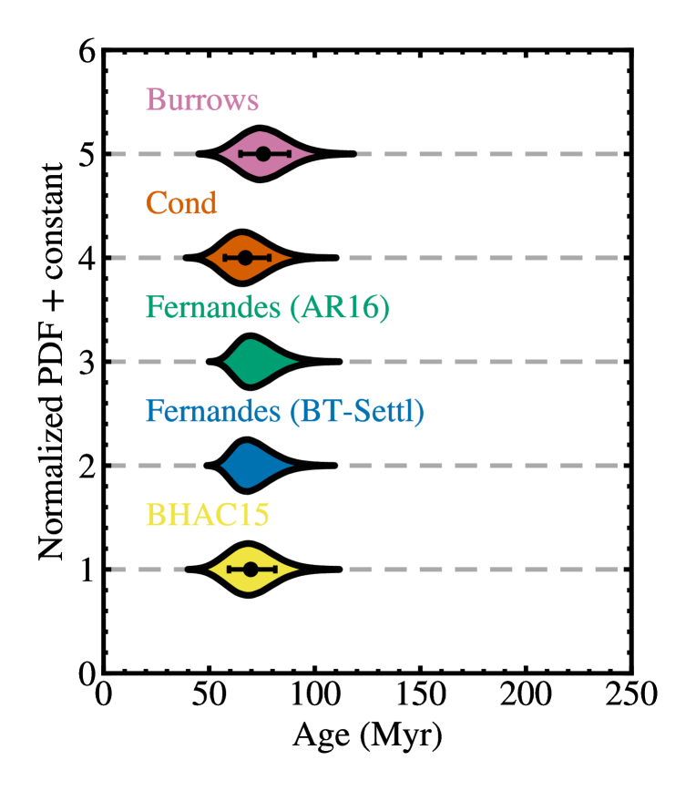
Figure 12: Predicted ages of HD 984 B based on the dynamical mass and luminosity for a variety of hot-start evolutionary models. Ages are inferred for a given model by sampling the luminosity and dynamical mass distributions of HD 984 B $10^{6}$ times, and then linearly interpolating the model grid to produce a corresponding age for each trial. Due to the partial coverage of the Fernandes et al. (2019) grids over HD 984 B’s luminosity and mass (see Figure 13), the corresponding predicted ages are somewhat overestimated for these models. Note that there is not a strict minimum age for these two models because the inferred age is luminosity-dependent. Altogether, hot-start models predict a young age of ${\sim}50{-}90$ Myr.

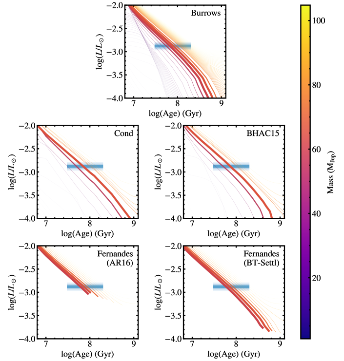
Figure 13: Iso-mass tracks from each evolutionary model considered in this study compared with HD 984 B’s age and luminosity. We adopt a linearly uniform distribution from 30–200 Myr for HD 984 B’s age and a Gaussian distribution for its luminosity. Contours of 1, 2, and $3\sigma$ are shown in blue. The color of the model tracks corresponds to their mass. The transparency and thickness of the tracks is related to the dynamical mass posterior probability density. The narrow dynamical mass distribution ($61\pm 4$ $\mathrm{M_{Jup}}$) means that only a few model tracks available from these grids appear thick in each panel. Note that the Fernandes et al. (2019) models only partially cover the luminosity, age, and dynamical mass of HD 984 B.

We employ a Monte Carlo approach to generate predicted mass distributions for each evolutionary model grid. The luminosity and age distributions of HD 984 B are first sampled $10^{6}$ times. The model grids are then linearly interpolated to produce a mass for each luminosity and age trial. We do not extrapolate outside of the model grids; this is pertinent to the Fernandes et al. (2019) models, which only cover a portion of HD 984 B’s luminosity and age range (see Figure 13). Solar metallicity grids are adopted for a uniform comparison of the models and because HD 984 is only slightly metal-rich ($\mathrm{[Fe/H]}=0.27$; Luck 2018). In the case of Fernandes et al. (2019), we compute predicted mass distributions for both BT-Settl and Aringer et al. (2016) model atmospheres.

Figure 11 shows the resulting inferred mass distributions for HD 984 B. The broad age constraint results in correspondingly broad predicted mass distributions for both models. Our dynamical mass measurement is consistent within $1\sigma$ of all model predictions. Note that the Fernandes et al. (2019) predicted mass distributions are limited to ${>}$57.6\text{\,}\mathrm{M}_{Jup}$$, which corresponds to the lowest mass track computed for those models. The Cond and BHAC15 inferred masses are similar, owing to their use of nearly identical interior structure models. The two atmospheric treatments with the Fernandes et al. (2019) grids also produce similar inferred masses. Overall, the broad age constraint for HD 984 limits detailed comparisons with evolutionary models. Improved age estimates would yield more precise inferred mass distributions and enable more rigorous model tests.

We also consider what ages the various models predict for HD 984 B given its dynamical mass and luminosity. Figure 12 shows the result of sampling the luminosity and dynamical mass distributions $10^{6}$ times through linear interpolation to find the corresponding age for each trial and model. Each model predicts a young age for HD 984 B of ${\sim}50{-}90$ Myr. This is consistent with the age constraint for HD 984 of $30{-}200$ Myr. If the true age of HD 984 is near the upper bound of that range, the companion could be overluminous, as was found for Gl 417 BC (Dupuy et al., 2014) and HD 130948 BC (Dupuy et al., 2009). Note again that the Fernandes et al. (2019) grids only partially cover the properties of HD 984 B, so the age distributions somewhat overestimate the predicted age for these two models. This is demonstrated in Figure 13, which displays the iso-mass tracks of each model against HD 984 B’s luminosity and age constraint.

4.4 Mass of HD 984 B

Our mass measurement of $61\pm 4$ $\mathrm{M_{Jup}}$ places HD 984 B well within the brown dwarf regime. The precise hydrogen burning limit (HBL), defined as the point where half of an object’s luminosity is generated via hydrogen fusion (Reid & Hawley, 2005), is a function of opacity (and by extension metallicity) and helium fraction (Burrows et al., 2001). Stars with higher opacities, metallicities, and helium fractions can sustain hydrogen burning at lower masses. For example, the CLES models (Scuflaire et al., 2008) upon which the Fernandes et al. (2019) models are based predict hydrogen burning mass limits that range from $78\text{\,}\mathrm{M}_{Jup}$ for $\mathrm{[Fe/H]}=+0.5$ to $84\text{\,}\mathrm{M}_{Jup}$ for $\mathrm{[Fe/H]}=-0.3$. The hydrogen burning limit can vary among models as well. For the CLES models, the substellar boundary is ${\sim}$82\text{\,}\mathrm{M}_{Jup}$$ for solar metallicity, while the BHAC15 models (Baraffe et al., 2015) produce a hydrogen burning limit of ${\sim}$73\text{\,}\mathrm{M}_{Jup}$$ and the Saumon & Marley (2008) models produce a limit of ${\sim}{$70\text{\,}\mathrm{M}_{Jup}$}$. Dupuy & Liu (2017) empirically constrained the substellar boundary to be $70\pm 4$ $\mathrm{M_{Jup}}$ by measuring dynamical masses of ultracool dwarf binaries. At a fiducial value of $75$ $\mathrm{M_{Jup}}$ for the HBL, HD 984 B’s dynamical mass places it in the brown dwarf regime to 99.7% significance. If instead we adopt a lower value of $70\text{\,}\mathrm{M}_{Jup}$ for the HBL, the significance drops slightly to 98.2%.

Among the small collection of substellar dynamical masses with well-constrained luminosities and ages (see Figure 1 and Table 1), HD 984 B is a young analog of several well-studied companions. HD 4113 C is a late T-dwarf benchmark companion with a similar measured mass of $66^{+5}_{-4}$ $\mathrm{M_{Jup}}$ (Cheetham et al., 2018). However, its dynamical mass is discrepant with the hot-start prediction of $36\pm 5$ $\mathrm{M_{Jup}}$, inferred via Cond models with a system age of $5^{+1.3}_{-1.7}$ Gyr. One possible explanation of this would be that HD 4113 C is an unresolved brown dwarf binary. Spectral fitting of this companion produces a radius of ${\sim}$1.5\text{\,}\mathrm{R}_{Jup}$$, which is significantly higher than expected for its effective temperature and age. The brown dwarf binary scenario could potentially resolve this tension as well, as it would produce higher radius estimates without significantly modifying the shape of the spectrum.

Another benchmark with a similar mass to HD 984 B but an older age is HD 4747 B. Discovered by Crepp et al. (2016), this companion is near the L/T transition (T$1\pm 2$; Crepp et al. 2018) with an age just under 4 Gyr. Its dynamical mass of $66.3^{+2.5}_{-3.0}$ $\mathrm{M_{Jup}}$ (Brandt et al., 2019) agrees well with hot-start model predictions with the exception of Burrows et al. (1997). Other model-independent masses near the substellar boundary include Gl 229 B ($71.4\pm 0.6$ $\mathrm{M_{Jup}}$; Nakajima et al. 1995; Brandt et al. 2021c), HD 72946 B ($72.5\pm 1.3$ $\mathrm{M_{Jup}}$; Bouchy et al. 2016; Brandt et al. 2021c), HR 7672 B ($72.7\pm 0.8$ $\mathrm{M_{Jup}}$; Liu et al. 2002; Crepp et al. 2012; Brandt et al. 2019), and HD 47127 B ($105^{+18}_{-27}$ $\mathrm{M_{Jup}}$; Bowler et al. 2021a). As additional dynamical masses are measured for objects with similar masses, the full evolution of brown dwarfs like HD 984 B will be progressively better constrained.

5 Conclusions

In this work, we measured the dynamical mass of the imaged substellar companion HD 984 B. Previous model-inferred masses that were based on the age and luminosity of the system ranged from 34 to 94 $\mathrm{M_{Jup}}$, which encompasses both the brown dwarf and stellar mass regimes. Our model-independent measurement of $61\pm 4$ $\mathrm{M_{Jup}}$ places the companion’s mass firmly in the brown dwarf regime (${\lesssim}75$ $\mathrm{M_{Jup}}$) to 99.7% significance. This dynamical mass was obtained by combining HD 984’s astrometric acceleration in the HGCA, new Keck/NIRC2 AO imaging of the companion, and RVs from HPF and HARPS. HD 984 B joins a small but growing list of benchmark substellar companions with measured dynamical masses and well-constrained ages and luminosities. Additional companion mass measurements spanning large regions of mass, age, and luminosity will enable holistic tests of substellar evolutionary models, ultimately improving our understanding of the formation and thermal evolution of brown dwarfs and giant planets.

References

- Allard & Hauschildt (1995) Allard, F., & Hauschildt, P. H. 1995, ApJ, 445, 433, doi: 10.1086/175708
- Allard et al. (2001) Allard, F., Hauschildt, P. H., Alexander, D. R., Tamanai, A., & Schweitzer, A. 2001, ApJ, 556, 357, doi: 10.1086/321547
- Allard et al. (2012a) Allard, F., Homeier, D., & Freytag, B. 2012a, RSPTA, 370, 2765, doi: 10.1098/rsta.2011.0269
- Allard et al. (2012b) Allard, F., Homeier, D., Freytag, B., & Sharp, C. 2012b, EAS Publications Series, 57, 3, doi: 10.1051/eas/1257001
- Amara & Quanz (2012) Amara, A., & Quanz, S. P. 2012, MNRAS, 427, 948, doi: 10.1111/j.1365-2966.2012.21918.x
- Aringer et al. (2016) Aringer, B., Girardi, L., Nowotny, W., Marigo, P., & Bressan, A. 2016, MNRAS, 457, 3611, doi: 10.1093/mnras/stw222
- Astropy Collaboration et al. (2013) Astropy Collaboration, Robitaille, T. P., Tollerud, E. J., et al. 2013, A&A, 558, A33, doi: 10.1051/0004-6361/201322068
- Astropy Collaboration et al. (2018) Astropy Collaboration, Price-Whelan, A. M., Sipőcz, B. M., et al. 2018, AJ, 156, 123, doi: 10.3847/1538-3881/aabc4f
- Baraffe et al. (2003) Baraffe, I., Chabrier, G., Barman, T. S., Allard, F., & Hauschildt, P. H. 2003, A&A, 402, 701, doi: 10.1051/0004-6361:20030252
- Baraffe et al. (2015) Baraffe, I., Homeier, D., Allard, F., & Chabrier, G. 2015, A&A, 577, A42, doi: 10.1051/0004-6361/201425481
- Beatty et al. (2018) Beatty, T. G., Morley, C. V., Curtis, J. L., et al. 2018, AJ, 156, 168, doi: 10.3847/1538-3881/aad697
- Bell et al. (2015) Bell, C. P. M., Mamajek, E. E., & Naylor, T. 2015, MNRAS, 454, 593, doi: 10.1093/mnras/stv1981
- Blunt et al. (2017) Blunt, S., Nielsen, E. L., De Rosa, R. J., et al. 2017, AJ, 153, 229, doi: 10.3847/1538-3881/aa6930
- Blunt et al. (2020) Blunt, S., Wang, J. J., Angelo, I., et al. 2020, AJ, 159, 89, doi: 10.3847/1538-3881/ab6663
- Boro Saikia et al. (2018) Boro Saikia, S., Marvin, C. J., Jeffers, S. V., et al. 2018, A&A, 616, A108, doi: 10.1051/0004-6361/201629518
- Bouchy et al. (2016) Bouchy, F., Ségransan, D., Díaz, R. F., et al. 2016, A&A, 585, A46, doi: 10.1051/0004-6361/201526347
- Bowler (2016) Bowler, B. P. 2016, PASP, 128, 102001, doi: 10.1088/1538-3873/128/968/102001
- Bowler et al. (2020) Bowler, B. P., Blunt, S. C., & Nielsen, E. L. 2020, AJ, 159, 63, doi: 10.3847/1538-3881/ab5b11
- Bowler et al. (2017) Bowler, B. P., Liu, M. C., Mawet, D., et al. 2017, AJ, 153, 18, doi: 10.3847/1538-3881/153/1/18
- Bowler et al. (2018) Bowler, B. P., Dupuy, T. J., Endl, M., et al. 2018, AJ, 155, 159, doi: 10.3847/1538-3881/aab2a6
- Bowler et al. (2021a) Bowler, B. P., Endl, M., Cochran, W. D., et al. 2021a, ApJ, 913, L26, doi: 10.3847/2041-8213/abfec8
- Bowler et al. (2021b) Bowler, B. P., Cochran, W. D., Endl, M., et al. 2021b, AJ, 161, 106, doi: 10.3847/1538-3881/abd243
- Bradley et al. (2019) Bradley, L., Sipőcz, B., Robitaille, T., et al. 2019, astropy/photutils: v0.7.2, Zenodo, doi: 10.5281/zenodo.3568287
- Brandt et al. (2021a) Brandt, G. M., Brandt, T. D., Dupuy, T. J., Li, Y., & Michalik, D. 2021a, AJ, 161, 179, doi: 10.3847/1538-3881/abdc2e
- Brandt et al. (2021b) Brandt, G. M., Brandt, T. D., Dupuy, T. J., Michalik, D., & Marleau, G.-D. 2021b, ApJ, 915, L16, doi: 10.3847/2041-8213/ac0540
- Brandt et al. (2021c) Brandt, G. M., Dupuy, T. J., Li, Y., et al. 2021c, arXiv:2109.07525 [astro-ph]. http://arxiv.org/abs/2109.07525
- Brandt (2018) Brandt, T. D. 2018, ApJS, 239, 31, doi: 10.3847/1538-4365/aaec06
- Brandt (2021) —. 2021, ApJS, 254, 42, doi: 10.3847/1538-4365/abf93c
- Brandt et al. (2019) Brandt, T. D., Dupuy, T. J., & Bowler, B. P. 2019, AJ, 158, 140, doi: 10.3847/1538-3881/ab04a8
- Brandt et al. (2020) Brandt, T. D., Dupuy, T. J., Bowler, B. P., et al. 2020, AJ, 160, 196, doi: 10.3847/1538-3881/abb45e
- Brandt et al. (2021d) Brandt, T. D., Dupuy, T. J., Li, Y., et al. 2021d, AJ, 162, 186, doi: 10.3847/1538-3881/ac042e
- Burrows et al. (2001) Burrows, A., Hubbard, W. B., Lunine, J. I., & Liebert, J. 2001, RvMp, 73, 719, doi: 10.1103/RevModPhys.73.719
- Burrows & Liebert (1993) Burrows, A., & Liebert, J. 1993, RvMp, 65, 301, doi: 10.1103/RevModPhys.65.301
- Burrows et al. (1997) Burrows, A., Marley, M., Hubbard, W. B., et al. 1997, ApJ, 491, 856, doi: 10.1086/305002
- Cardoso (2012) Cardoso, C. V. V. 2012, PhDT, Univ of Exeter
- Casagrande et al. (2011) Casagrande, L., Schönrich, R., Asplund, M., et al. 2011, A&A, 530, A138, doi: 10.1051/0004-6361/201016276
- Chabrier et al. (2000) Chabrier, G., Baraffe, I., Allard, F., & Hauschildt, P. 2000, ApJ, 542, 464, doi: 10.1086/309513
- Chabrier et al. (2014) Chabrier, G., Johansen, A., Janson, M., & Rafikov, R. 2014, in Protostars and Planets VI (University of Arizona Press), doi: 10.2458/azu_uapress_9780816531240-ch027
- Chabrier et al. (2019) Chabrier, G., Mazevet, S., & Soubiran, F. 2019, ApJ, 872, 51, doi: 10.3847/1538-4357/aaf99f
- Cheetham et al. (2018) Cheetham, A., Ségransan, D., Peretti, S., et al. 2018, A&A, 614, A16, doi: 10.1051/0004-6361/201630136
- Chowdhury et al. (2021) Chowdhury, S., Banerjee, P., Garain, D., & Sarkar, T. 2021, arXiv:2107.02691 [astro-ph, physics:gr-qc]. http://arxiv.org/abs/2107.02691
- Craig et al. (2017) Craig, M., Crawford, S., Seifert, M., et al. 2017, astropy/ccdproc: v1.3.0.post1, Zenodo, doi: 10.5281/zenodo.1069648
- Crepp et al. (2016) Crepp, J. R., Gonzales, E. J., Bechter, E. B., et al. 2016, ApJ, 831, 136, doi: 10.3847/0004-637X/831/2/136
- Crepp et al. (2012) Crepp, J. R., Johnson, J. A., Fischer, D. A., et al. 2012, ApJ, 751, 97, doi: 10.1088/0004-637X/751/2/97
- Crepp et al. (2018) Crepp, J. R., Principe, D. A., Wolff, S., et al. 2018, ApJ, 853, 192, doi: 10.3847/1538-4357/aaa2fd
- Crockett et al. (2012) Crockett, C. J., Mahmud, N. I., Prato, L., et al. 2012, ApJ, 761, 164, doi: 10.1088/0004-637X/761/2/164
- Currie et al. (2020) Currie, T., Brandt, T. D., Kuzuhara, M., et al. 2020, ApJ, 904, L25, doi: 10.3847/2041-8213/abc631
- Desrochers et al. (2018) Desrochers, M.-E., Artigau, É., Gagné, J., et al. 2018, ApJ, 852, 55, doi: 10.3847/1538-4357/aa9e86
- Dieterich et al. (2018) Dieterich, S. B., Weinberger, A. J., Boss, A. P., et al. 2018, ApJ, 865, 28, doi: 10.3847/1538-4357/aadadc
- Dupuy et al. (2019) Dupuy, T. J., Brandt, T. D., Kratter, K. M., & Bowler, B. P. 2019, ApJL, 871, L4, doi: 10.3847/2041-8213/aafb31
- Dupuy & Liu (2017) Dupuy, T. J., & Liu, M. C. 2017, ApJS, 231, 15, doi: 10.3847/1538-4365/aa5e4c
- Dupuy et al. (2009) Dupuy, T. J., Liu, M. C., & Ireland, M. J. 2009, ApJ, 692, 729, doi: 10.1088/0004-637X/692/1/729
- Dupuy et al. (2014) —. 2014, ApJ, 790, 133, doi: 10.1088/0004-637X/790/2/133
- ESA (1997) ESA, ed. 1997, ESA Special Publication, Vol. 1200, The HIPPARCOS and TYCHO catalogues. Astrometric and photometric star catalogues derived from the ESA HIPPARCOS Space Astrometry Mission
- Fernandes et al. (2019) Fernandes, C. S., Van Grootel, V., Salmon, S. J. A. J., et al. 2019, ApJ, 879, 94, doi: 10.3847/1538-4357/ab2333
- Filippazzo et al. (2015) Filippazzo, J. C., Rice, E. L., Faherty, J., et al. 2015, ApJ, 810, 158, doi: 10.1088/0004-637X/810/2/158
- Foreman-Mackey (2016) Foreman-Mackey, D. 2016, JOSS, 1, 24, doi: 10.21105/joss.00024
- Foreman-Mackey et al. (2013) Foreman-Mackey, D., Hogg, D. W., Lang, D., & Goodman, J. 2013, PASP, 125, 306, doi: 10.1086/670067
- Fortney et al. (2008) Fortney, J. J., Marley, M. S., Saumon, D., & Lodders, K. 2008, ApJ, 683, 1104, doi: 10.1086/589942
- Gagné et al. (2016) Gagné, J., Plavchan, P., Gao, P., et al. 2016, ApJ, 822, 40, doi: 10.3847/0004-637X/822/1/40
- Gagné et al. (2018) Gagné, J., Mamajek, E. E., Malo, L., et al. 2018, ApJ, 856, 23, doi: 10.3847/1538-4357/aaae09
- Gaia Collaboration et al. (2020) Gaia Collaboration, Brown, A. G., Vallenari, A., Prusti, T., & de Bruijne, J. H. 2020, A&A, doi: 10.1051/0004-6361/202039657
- Gelman & Rubin (1992) Gelman, A., & Rubin, D. B. 1992, StaSc, 7, 457, doi: 10.1214/ss/1177011136
- Gharib-Nezhad et al. (2021) Gharib-Nezhad, E., Marley, M. S., Batalha, N. E., et al. 2021, ApJ, 919, 21, doi: 10.3847/1538-4357/ac0a7d
- Gomez Gonzalez et al. (2016) Gomez Gonzalez, C. A., Absil, O., Absil, P.-A., et al. 2016, A&A, 589, A54, doi: 10.1051/0004-6361/201527387
- Gomez Gonzalez et al. (2017) Gomez Gonzalez, C. A., Wertz, O., Absil, O., et al. 2017, AJ, 154, 7, doi: 10.3847/1538-3881/aa73d7
- Grandjean et al. (2020) Grandjean, A., Lagrange, A.-M., Keppler, M., et al. 2020, A&A, 633, A44, doi: 10.1051/0004-6361/201936038
- Harris et al. (2020) Harris, C. R., Millman, K. J., van der Walt, S. J., et al. 2020, Nature, 585, 357, doi: 10.1038/s41586-020-2649-2
- Hauschildt et al. (1999) Hauschildt, P. H., Allard, F., & Baron, E. 1999, ApJ, 512, 377, doi: 10.1086/306745
- Hunter (2007) Hunter, J. D. 2007, CSE, 9, 90, doi: 10.1109/MCSE.2007.55
- Høg et al. (2000) Høg, E., Fabricius, C., Makarov, V. V., et al. 2000, A&A, 355, L27
- Ireland et al. (2008) Ireland, M. J., Kraus, A., Martinache, F., Lloyd, J. P., & Tuthill, P. G. 2008, ApJ, 678, 463, doi: 10.1086/529578
- Johnson-Groh et al. (2017) Johnson-Groh, M., Marois, C., De Rosa, R. J., et al. 2017, AJ, 153, 190, doi: 10.3847/1538-3881/aa6480
- Kanodia & Wright (2018) Kanodia, S., & Wright, J. 2018, RNAAS, 2, 4, doi: 10.3847/2515-5172/aaa4b7
- King et al. (2010) King, R. R., McCaughrean, M. J., Homeier, D., et al. 2010, A&A, 510, A99, doi: 10.1051/0004-6361/200912981
- Kraft (1967) Kraft, R. P. 1967, ApJ, 150, 551, doi: 10.1086/149359
- Kratter et al. (2010) Kratter, K. M., Murray-Clay, R. A., & Youdin, A. N. 2010, ApJ, 710, 1375, doi: 10.1088/0004-637X/710/2/1375
- Kumar (1963) Kumar, S. S. 1963, ApJ, 137, 1121, doi: 10.1086/147589
- Lagrange et al. (2010) Lagrange, A.-M., Bonnefoy, M., Chauvin, G., et al. 2010, Sci, 329, 57, doi: 10.1126/science.1187187
- Lightkurve Collaboration et al. (2018) Lightkurve Collaboration, Cardoso, J. V. d. M., Hedges, C., et al. 2018, Lightkurve: Kepler and TESS time series analysis in Python
- Lindegren (2018) Lindegren, L. 2018, Re-normalising the astrometric chi-square in Gaia DR2, Tech. Rep. GAIA-C3-TN-LU-LL-124-01. http://www.rssd.esa.int/doc_fetch.php?id=3757412
- Liu (2004) Liu, M. C. 2004, Sci, 305, 1442, doi: 10.1126/science.1102929
- Liu et al. (2002) Liu, M. C., Fischer, D. A., Graham, J. R., et al. 2002, ApJ, 571, 519, doi: 10.1086/339845
- Luck (2018) Luck, R. E. 2018, AJ, 155, 111, doi: 10.3847/1538-3881/aaa9b5
- Lucy & Sweeney (1971) Lucy, L. B., & Sweeney, M. A. 1971, AJ, 76, 544, doi: 10.1086/111159
- Macintosh et al. (2015) Macintosh, B., Graham, J. R., Barman, T., et al. 2015, Sci, 350, 64, doi: 10.1126/science.aac5891
- Mahadevan et al. (2012) Mahadevan, S., Ramsey, L., Bender, C., et al. 2012, in Proc. SPIE, Vol. 8446, Ground-based and Airborne Instrumentation for Astronomy IV, ed. I. S. McLean, S. K. Ramsay, & H. Takami, Amsterdam, Netherlands, 84461S, doi: 10.1117/12.926102
- Mahadevan et al. (2014) Mahadevan, S., Ramsey, L. W., Terrien, R., et al. 2014, in Proc. SPIE, Vol. 9147, Ground-based and Airborne Instrumentation for Astronomy V, ed. S. K. Ramsay, I. S. McLean, & H. Takami, 91471G, doi: 10.1117/12.2056417
- Mamajek & Hillenbrand (2008) Mamajek, E. E., & Hillenbrand, L. A. 2008, ApJ, 687, 1264, doi: 10.1086/591785
- Marleau & Cumming (2014) Marleau, G.-D., & Cumming, A. 2014, MNRAS, 437, 1378, doi: 10.1093/mnras/stt1967
- Marley & Robinson (2015) Marley, M., & Robinson, T. 2015, ARA&A, 53, 279, doi: 10.1146/annurev-astro-082214-122522
- Marley et al. (2007) Marley, M. S., Fortney, J. J., Hubickyj, O., Bodenheimer, P., & Lissauer, J. J. 2007, ApJ, 655, 541, doi: 10.1086/509759
- Marley et al. (1996) Marley, M. S., Saumon, D., Guillot, T., et al. 1996, Sci, 272, 1919, doi: 10.1126/science.272.5270.1919
- Marois et al. (2006) Marois, C., Lafrenière, D., Doyon, R., Macintosh, B., & Nadeau, D. 2006, ApJ, 641, 556, doi: 10.1086/500401
- Marois et al. (2010) Marois, C., Zuckerman, B., Konopacky, Q. M., Macintosh, B., & Barman, T. 2010, Nature, 468, 1080, doi: 10.1038/nature09684
- Mayor et al. (2003) Mayor, M., Pepe, F., Queloz, D., et al. 2003, Msngr, 114, 20
- McKinney (2010) McKinney, W. 2010, in Proceedings of the 9th Python in Sci Conference, Austin, Texas, 56–61, doi: 10.25080/Majora-92bf1922-00a
- Meshkat et al. (2015) Meshkat, T., Bonnefoy, M., Mamajek, E. E., et al. 2015, MNRAS, 453, 2378, doi: 10.1093/mnras/stv1732
- Metcalf et al. (2019) Metcalf, A. J., Anderson, T., Bender, C. F., et al. 2019, Optic, 6, 233, doi: 10.1364/OPTICA.6.000233
- Mints & Hekker (2017) Mints, A., & Hekker, S. 2017, A&A, 604, A108, doi: 10.1051/0004-6361/201630090
- Mordasini (2013) Mordasini, C. 2013, A&A, 558, A113, doi: 10.1051/0004-6361/201321617
- Morzinski et al. (2015) Morzinski, K. M., Males, J. R., Skemer, A. J., et al. 2015, ApJ, 815, 108, doi: 10.1088/0004-637X/815/2/108
- Nakajima et al. (1995) Nakajima, T., Oppenheimer, B. R., Kulkarni, S. R., et al. 1995, Nature, 378, 463, doi: 10.1038/378463a0
- Nelder & Mead (1965) Nelder, J. A., & Mead, R. 1965, CompJ, 7, 308, doi: 10.1093/comjnl/7.4.308
- Nielsen et al. (2019) Nielsen, E. L., De Rosa, R. J., Macintosh, B., et al. 2019, AJ, 158, 13, doi: 10.3847/1538-3881/ab16e9
- Ninan et al. (2018) Ninan, J. P., Bender, C. F., Mahadevan, S., et al. 2018, in Proc. SPIE, Vol. 10709, High Energy, Optical, and Infrared Detectors for Astronomy VIII, ed. A. D. Holland & J. Beletic, 107092U, doi: 10.1117/12.2312787
- Nowak et al. (2020) Nowak, M., Lacour, S., Lagrange, A.-M., et al. 2020, A&A, 642, L2, doi: 10.1051/0004-6361/202039039
- Phillips et al. (2020) Phillips, M. W., Tremblin, P., Baraffe, I., et al. 2020, A&A, 637, A38, doi: 10.1051/0004-6361/201937381
- Raposo-Pulido & Peláez (2017) Raposo-Pulido, V., & Peláez, J. 2017, MNRAS, 467, 1702, doi: 10.1093/mnras/stx138
- Reid & Hawley (2005) Reid, I. N., & Hawley, S. L. 2005, New light on dark stars : red dwarfs, low-mass stars, brown dwarfs, doi: 10.1007/3-540-27610-6
- Ren et al. (2018) Ren, B., Pueyo, L., Zhu, G. B., Debes, J., & Duchêne, G. 2018, ApJ, 852, 104, doi: 10.3847/1538-4357/aaa1f2
- Ricker et al. (2014) Ricker, G. R., Winn, J. N., Vanderspek, R., et al. 2014, Journal of Astronomical Telescopes, Instruments, and Systems, 1, 014003, doi: 10.1117/1.JATIS.1.1.014003
- Saumon et al. (1995) Saumon, D., Chabrier, G., & van Horn, H. M. 1995, ApJS, 99, 713, doi: 10.1086/192204
- Saumon et al. (1996) Saumon, D., Hubbard, W. B., Burrows, A., et al. 1996, ApJ, 460, 993, doi: 10.1086/177027
- Saumon & Marley (2008) Saumon, D., & Marley, M. S. 2008, ApJ, 689, 1327, doi: 10.1086/592734
- Scuflaire et al. (2008) Scuflaire, R., Théado, S., Montalbán, J., et al. 2008, Ap&SS, 316, 83, doi: 10.1007/s10509-007-9650-1
- Service et al. (2016) Service, M., Lu, J. R., Campbell, R., et al. 2016, PASP, 128, 095004, doi: 10.1088/1538-3873/128/967/095004
- Shetrone et al. (2007) Shetrone, M., Cornell, M., Fowler, J., et al. 2007, PASP, 119, 556, doi: 10.1086/519291
- Skrutskie et al. (2006) Skrutskie, M. F., Cutri, R. M., Stiening, R., et al. 2006, AJ, 131, 1163, doi: 10.1086/498708
- Soummer et al. (2012) Soummer, R., Pueyo, L., & Larkin, J. 2012, ApJ, 755, L28, doi: 10.1088/2041-8205/755/2/L28
- Spiegel & Burrows (2012) Spiegel, D. S., & Burrows, A. 2012, ApJ, 745, 174, doi: 10.1088/0004-637X/745/2/174
- Spiegel et al. (2011) Spiegel, D. S., Burrows, A., & Milsom, J. A. 2011, ApJ, 727, 57, doi: 10.1088/0004-637X/727/1/57
- Stanford-Moore et al. (2020) Stanford-Moore, S. A., Nielsen, E. L., De Rosa, R. J., Macintosh, B., & Czekala, I. 2020, ApJ, 898, 27, doi: 10.3847/1538-4357/ab9a35
- Stassun et al. (2006) Stassun, K. G., Mathieu, R. D., & Valenti, J. A. 2006, Nature, 440, 311, doi: 10.1038/nature04570
- Stassun & Torres (2021) Stassun, K. G., & Torres, G. 2021, ApJ, 907, L33, doi: 10.3847/2041-8213/abdaad
- Stefansson et al. (2016) Stefansson, G., Hearty, F., Robertson, P., et al. 2016, ApJ, 833, 175, doi: 10.3847/1538-4357/833/2/175
- Tofflemire et al. (2021) Tofflemire, B. M., Rizzuto, A. C., Newton, E. R., et al. 2021, AJ, 161, 171, doi: 10.3847/1538-3881/abdf53
- Torres et al. (2008) Torres, C. A. O., Quast, G. R., Melo, C. H. F., & Sterzik, M. F. 2008, in Handbook of Star Forming Regions, Volume II, ed. B. Reipurth, Vol. 5, 757. https://ui.adsabs.harvard.edu/abs/2008hsf2.book..757T
- Tran et al. (2021) Tran, Q. H., Bowler, B. P., Cochran, W. D., et al. 2021, AJ, 161, 173, doi: 10.3847/1538-3881/abe041
- Triaud et al. (2020) Triaud, A. H. M. J., Burgasser, A. J., Burdanov, A., et al. 2020, Nature Astronomy, 4, 650, doi: 10.1038/s41550-020-1018-2
- van der Walt et al. (2014) van der Walt, S., Schönberger, J. L., Nunez-Iglesias, J., et al. 2014, PeerJ, 2, e453, doi: 10.7717/peerj.453
- van Leeuwen (2007) van Leeuwen, F. 2007, A&A, 474, 653, doi: 10.1051/0004-6361:20078357
- van Dokkum (2001) van Dokkum, P. 2001, PASP, 113, 1420, doi: 10.1086/323894
- Vigan et al. (2017) Vigan, A., Bonavita, M., Biller, B., et al. 2017, A&A, 603, A3, doi: 10.1051/0004-6361/201630133
- Virtanen et al. (2020) Virtanen, P., Gommers, R., Oliphant, T. E., et al. 2020, Nature Methods, 17, 261, doi: 10.1038/s41592-019-0686-2
- Voges et al. (1999) Voges, W., Aschenbach, B., Boller, T., et al. 1999, A&A, 349, 389
- White et al. (2007) White, R. J., Gabor, J. M., & Hillenbrand, L. A. 2007, AJ, 133, 2524, doi: 10.1086/514336
- Wizinowich (2013) Wizinowich, P. 2013, PASP, 125, 798, doi: 10.1086/671425
- Zechmeister et al. (2018) Zechmeister, M., Reiners, A., Amado, P. J., et al. 2018, A&A, 609, A12, doi: 10.1051/0004-6361/201731483
- Zhang et al. (2021) Zhang, Z., Liu, M. C., Claytor, Z. R., et al. 2021, ApJ, 916, L11, doi: 10.3847/2041-8213/ac1123
- Zuckerman et al. (2011) Zuckerman, B., Rhee, J. H., Song, I., & Bessell, M. S. 2011, ApJ, 732, 61, doi: 10.1088/0004-637X/732/2/61
- Zúñiga-Fernández et al. (2021) Zúñiga-Fernández, S., Bayo, A., Elliott, P., et al. 2021, A&A, 645, A30, doi: 10.1051/0004-6361/202037830