Wide binaries from the H3 survey: the thick disk and halo have similar wide binary fractions
Abstract
Due to the different environments in the Milky Way’s disk and halo, comparing wide binaries in the disk and halo is key to understanding wide binary formation and evolution. By using Gaia Early Data Release 3, we search for resolved wide binary companions in the H3 survey, a spectroscopic survey that has compiled 150,000 spectra for thick-disk and halo stars to date. We identify 800 high-confidence (a contamination rate of 4%) wide binaries and two resolved triples, with binary separations mostly between - AU and a lowest [Fe/H] of . Based on their Galactic kinematics, 33 of them are halo wide binaries, and most of those are associated with the accreted Gaia-Sausage-Enceladus galaxy. The wide binary fraction in the thick disk decreases toward the low metallicity end, consistent with the previous findings for the thin disk. Our key finding is that the halo wide binary fraction is consistent with the thick-disk stars at a fixed [Fe/H]. There is no significant dependence of the wide binary fraction on the -captured abundance. Therefore, the wide binary fraction is mainly determined by the iron abundance, not their disk or halo origin nor the -captured abundance. Our results suggest that the formation environments play a major role for the wide binary fraction, instead of other processes like radial migration that only apply to disk stars.
1 Introduction
Since wide binaries are weakly bound, they are sensitive to their formation and evolution environments. Wide binary fractions reflect the density of star formation environments because dense environments like star clusters can easily disrupt wide binaries and thus reduce wide binary formation (Scally et al., 1999; Parker et al., 2009; Geller et al., 2019; Deacon & Kraus, 2020). In the Milky Way disk, gravitational interactions with passing stars, molecular clouds, and the Galactic tide can disrupt wide binaries at separations AU, providing a unique probe for pc-scale gravitational fields (Retterer & King, 1982; Bahcall et al., 1985; Weinberg et al., 1987; Jiang & Tremaine, 2010). In the halo where the interactions with passing stars and molecular clouds are less important, halo wide binaries provide a critical constraint on the nature of dark matter (Chaname & Gould, 2004; Quinn et al., 2009; Carr & Kühnel, 2020). Now with an increasing number of disrupted accreted galaxies found in the Milky Way’s stellar halo (Belokurov et al., 2018; Helmi et al., 2018; Conroy et al., 2019a; Li et al., 2019; Belokurov et al., 2020; Naidu et al., 2020, see review by Helmi 2020), halo wide binaries are critical in constraining wide binary formation and the formation environments of these progenitor dwarf galaxies in the early Universe.
Our recent work shows that the wide binary fraction (defined at - AU) in the disk peaks at the solar metallicity and decreases both toward the low- and high-metallicity ends (Hwang et al., 2021). We propose several hypotheses that may explain the non-monotonic metallicity dependence, including the different stellar density in the formation environments at different epochs (Harris & Pudritz, 1994; Elmegreen & Efremov, 1997; Kravtsov & Gnedin, 2005; Kruijssen, 2014; Ma et al., 2020), the dynamical unfolding of compact triples (Reipurth & Mikkola, 2012; Elliott & Bayo, 2016), and the radial migration of Galactic orbits (Sellwood & Binney, 2002). In the radial migration scenario, stars with supersolar and subsolar metallicities are formed at other Galactocentric radii and then migrated to the solar neighborhood. Then the lower wide binary fraction at supersolar and subsolar metallicities may be due to the different formation environments at different Galactocentric radii, or due to that the radial migration process (e.g. the enhanced interaction with molecular clouds) can efficiently disrupt wide binaries.
To constrain these hypotheses, comparing properties of binaries in the disk and the halo is particularly valuable because they probe a very different metallicity range, formation environments, stellar ages, and evolution environments. In particular, halo stars do not experience radial migration in the Milky Way disk, and thus halo wide binaries do not get disrupted by the radial migration process. Therefore, if radial migration plays an important role in the wide binary fraction, we would expect a higher wide binary fraction in the halo than in the disk.
Despite their importance, halo wide binaries have been challenging to identify in the past. First, the density of halo stars is low compared to that of the disk in the solar neighborhood, comprising less than 0.2 per cent of local stars (Helmi, 2008). Therefore, assembling a large and clean halo star sample is not straightforward. Second, identifying a resolved companion as the wide binary companion was difficult before the Gaia era. Even though the Gaia mission provides the proper motions and parallaxes for billions of stars (Gaia Collaboration et al., 2016), most of the wide binary samples are still limited within 1 kpc (El-Badry & Rix, 2018; Hartman & Lépine, 2020; El-Badry et al., 2021). Furthermore, most of these wide binaries do not have radial velocities available from Gaia, making differentiating disk and halo stars challenging. Therefore, the number of robustly identified halo wide binaries remains insufficient to place a useful constraint on the halo wide binary fraction (Hwang et al., 2021).
In this paper, we overcome these difficulties by having a customized wide binary search for stars in the H3 survey. The H3 survey is a large spectroscopic survey targeting halo and thick-disk stars (Conroy et al., 2019b). There are H3 stars in our current analysis, and it is expected to have 300,000 stars at the end of the survey, with about 20% of them being halo stars. The high-precision radial velocities measured from H3 are critical to differentiate disk and halo stars by their Galactic kinematics. Since most of the H3 stars are more than 1 kpc away, we optimize the wide binary method for the H3 stars to maximize the resulting information. With the H3 wide binaries, we investigate the difference in the wide binary fractions of the halo and the disk to understand the formation and evolution of wide binaries.
The paper is structured as follows. Sec. 2 describes the H3 and Gaia dataset and the general criteria for the sample selection. Sec. 3 details the method of wide binary search and presents the results. Sec. 4 explores the properties of the wide binary candidates, and Sec. 5 investigates the metallicity dependence of the wide binary fraction. We then discuss the implications in Sec. 6 and conclude in Sec. 7. Throughout the paper, we use ‘wide binaries’ and ‘wide binary candidates’ interchangeably when referring to the selected wide binaries. We use ‘metallicity’ and ‘iron abundance’ ([Fe/H]) interchangeably and always refer to [/Fe] as -captured abundances. We use the notation ‘binary’ even if some of them can be unresolved triples.
2 Sample selection
2.1 H3 survey
The H3 (‘Hectochelle in the Halo at High Resolution’) survey is a high-resolution spectroscopic () survey targeting thick-disk and halo stars (Conroy et al., 2019b). The survey is conducted by the 6.5-m MMT with a wavelength coverage of 5150-5300Å. The survey has been collecting data since 2017. The main selection of H3 is composed of the following criteria: (1) where is the band magnitude from Pan-STARRS (Chambers et al., 2016; Flewelling et al., 2016); (2) mas (later changed to ) where and are parallaxes and parallax uncertainties from Gaia Data Release 2 (Gaia Collaboration et al., 2018); (3) to increase the halo star fraction; (4) declination to be observable from MMT. The H3 survey has secondary selections targeting stellar streams, K giants, blue horizontal branch stars, and RR Lyrae. This simple selection of magnitudes and parallaxes provides an unbiased view of the distant Milky Way.
The stellar parameters are measured from the H3 spectra using MINESweeper (Cargile et al., 2020). MINESweeper is a Bayesian framework that incorporates the information from H3 spectra, broadband photometry, and priors like Gaia parallaxes to fit stellar models computed by MIST (v2.0) (Dotter, 2016; Choi et al., 2016, Dotter et al. in preparation). Cargile et al. (2020) show that the stellar parameters of benchmark stars and clusters measured by MINESweeper are in good agreement with literature values.
In this paper, we use the radial velocities, distances, surface iron abundances ([Fe/H]), surface -captured elemental abundances ([/Fe]), and extinction () measured from MINESweeper. The surface elemental abundances may differ from the initial abundances due to atomic diffusion and mixing. By including the model from Dotter et al. (2017), MINESweeper derives the initial chemical abundances, denoted as [Fe/H]init and [/Fe]init. The difference between [Fe/H] and [Fe/H]init depends on the evolutionary stages, stellar ages, and initial metallicities, with the largest difference of dex happening at the main-sequence turnoff of metal-poor stars (Dotter et al., 2017). In our sample, the median difference between [Fe/H] and [Fe/H]init is 0.1 dex, and we do not find significant changes in our results between them. We present our results using surface abundances for better comparison with the literature. The -captured elemental abundances from MINESweeper scale the -elements O, Ne, Mg, Si, S, Ca, and Ti, and the measurement is most sensitive to [Mg/Fe] due to H3’s wavelength coverage of Mg I triplet (Cargile et al., 2020).
In this paper, we use the proprietary H3 data from rcat_V4.0.3.d20201031_MSG.fits, with data collected between September 2017 and October 2020. We require FLAG==0 and signal-to-noise ratios (SNR) to avoid unreliable stellar parameter measurements. Targets from the Sagittarius stream (Sgr_FLAG==1 from Johnson et al. 2020) and tiles specifically for streams (tileID starting with ‘tb’) are excluded because stream members moving in similar directions may increase the chance-alignment probability. For stars that were observed by H3 multiple times, we use the entries with the highest SNR. These selections result in a parent sample of 100,967 unique H3 stars for wide binary search. In this sample, the median uncertainty is 0.05 dex for [Fe/H], 0.05 dex for [/Fe], 0.2 km s-1 for radial velocities, and 6% for distances.
2.2 Gaia survey
Gaia is an all-sky survey that provides optical broad-band photometry and high-precision astrometric measurements (Gaia Collaboration et al., 2016). Gaia Early Data Release 3 (EDR3) (Gaia Collaboration et al., 2020) was released in December 2020, with parallaxes and proper motions available for 1.5 billion sources down to Gaia G-band magnitudes of mag. In addition, Gaia measures radial velocities for bright stars ( mag for EDR3, and may reach mag by the end of mission), but most halo stars are fainter than this magnitude limit. This is one of the H3 survey’s motivations to target for stars fainter than 15 mag. We use Gaia EDR3 to search for the comoving companions around the H3 stars. Because H3 target selection uses Gaia’s parallaxes which are derived together with proper motions, all H3 targets have proper motions from Gaia.
The goal of this paper is to search for H3 stars’ resolved wide companions that have nearly identical Gaia proper motions as the H3 targets. We query a field star sample from Gaia EDR3 to conduct the wide binary search. For this field star sample, we require that their proper motions be available in Gaia EDR3 (astrometric_params_solved or 95). We do not apply any criteria on magnitudes and astrometric quality indicators (e.g. ruwe) to maximize the chance of finding the companions. Our wide binary selection compares the proper motions for each pair, which implicitly requires good astrometric quality, and it is inevitable that we may miss some genuine wide binaries because some of their stars have worse astrometric quality.
Gaia EDR3’s ability to resolve close pairs starts dropping significantly below 0.7″, and only about 50% of pairs can be spatially resolved at 0.5″ (Fabricius et al., 2020). We do not use Gaia’s BP-RP colors for our wide binary selection, but we use them when investigating the properties of the selected wide binaries. When BP-RP colors are used in the analysis, we require their bp_flux_over_error and rp_flux_over_error to be larger than 10. Unlike G-band photometry, BP and RP fluxes do not have de-blending treatment, and therefore their fluxes can be affected by nearby sources within about 2″ (Riello et al., 2021). To ensure that BP-RP colors are not strongly affected by the nearby sources, we apply an additional criterion of phot_bp_rp_excess_factor when BP-RP colors are used in the analysis.
2.3 Calculations of Galactic kinematics
Radial velocities from the H3 survey are necessary for computing Galactic kinematics parameters and to differentiating disk and halo stars. We measure the parameters for Galactic kinematics, including the total energy () and the angular momentum along the Galactic -direction (), using Gala v1.1 (Price-Whelan et al., 2020). We use the Galactocentric frame from Astropy v4.0 (Astropy Collaboration et al., 2013, 2018): Sun’s Galactocentric radius kpc (Gravity Collaboration et al., 2018), solar motion with respect to the local standard of rest [, , ]=[, , ] km s-1(Drimmel & Poggio, 2018), and Sun’s current Galactic height pc (Bennett & Bovy, 2019). The Milky Way potential MilkyWayPotential (Bovy, 2015) is adopted. and are used to separate halo and disk stars, and using different Milky Way potential models does not affect this selection significantly (Naidu et al., 2020). A right-handed coordinate is used, and thus a star on a prograde (retrograde) orbit has a negative (positive) . The Galactic orbit is integrated for 25 Gyr with a time step of 1 Myr using the Dormand & Prince (1978) integration scheme. The eccentricity of Galactic orbits is then derived from where and are the apocenter and pericenter of the Galactic orbit.
The observational inputs for kinematic parameter calculations are the radial velocities and distances measured from H3 spectra using MINESweeper, and celestial coordinates and astrometric solutions measured from Gaia EDR3. Following Naidu et al. (2020), when and are used in the analysis, we require that (i) ; or (ii) km2 s-2 kpc km s-1, where ‘’ is the Boolean ‘and’ operator. The first condition is a normal 3- uncertainty cut, and the second condition is to ensure that we keep halo stars with small in the sample (otherwise they may be excluded by the 3- uncertainty cut). Out of 100,967 H3 stars, 99,161 (98 per cent) of them satisfy these kinematic criteria.
3 Wide binary search
For a solar-mass wide binary with a semi-major axis of AU, its orbital Keplerian velocity is km s-1. Therefore, two resolved stars in a wide binary would have nearly identical proper motions. For a given H3 star and a nearby star from Gaia, we compute the proper motion difference by
| (1) |
where and are the Gaia EDR3 proper motions in right ascension direction () and in declination direction () for star ( or 1), respectively. With Gaia’s proper motion precision at the relevant magnitudes, the typical uncertainties of is mas yr-1. The relative velocity difference projected in the plane of sky is , where is in units of km s-1, is in units of mas yr-1, is the heliocentric distance of the pair in kpc, and the factor of 4.74 is from the unit conversion. Therefore, for a wide binary at distances of 1 to 10 kpc, Gaia can measure the difference in the projected orbital velocity with uncertainties of km s-1. This precision is sufficient to distinguish genuine wide binaries where the orbital velocities are km s-1 from random chance-alignment pairs where the typical velocity differences are km s-1 for the thick-disk and halo stars.
For every H3 target, we search for a possible resolved wide companion in Gaia within 60 arcsec. In most cases, radial velocities are only available for H3 targets but not for Gaia field stars, so we cannot compute radial velocity difference for the pair to help the binary search. Furthermore, limited by the fiber allocation, the minimum angular separation between two H3 stars is 20 arcsec, making the wide binary search among H3 stars (when both stars were observed by H3) difficult to result in a statistically useful sample. Most H3 targets are distant ( kpc) and therefore they do not have precise distances from Gaia EDR3. The precision of the distance measurement from Gaia and the MINESweeper fit is not sufficient to distinctly separate the wide binary population from the random chance-alignment pairs in the relative velocity-physical separation space (e.g. Hwang et al. 2020). Without distances, proper motion differences and angular separations cannot be converted to projected relative velocity differences and physical separations. Therefore, we search the wide binaries in the proper motion difference-angular separation space. The advantage is that their measurement uncertainties are nearly negligible ( mas for angular separations and mas yr-1 for proper motion differences), with the caveat that the search has different sensitivities for binary’s physical separations at different distances.
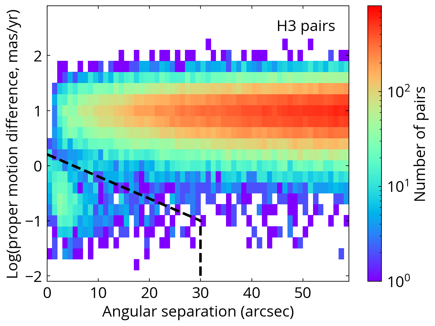
Fig. 1 (left panel) shows the proper motion differences and angular separations of all the H3-Gaia pairs. To reduce the contamination, we require that the parallax difference of the pair is consistent with zero within . An enhanced population with separations arcsec and proper motion differences mas yr-1can be seen, indicative of the resolved wide binary populations. The rest of the pairs in the upper-right part of the plot are chance alignments.
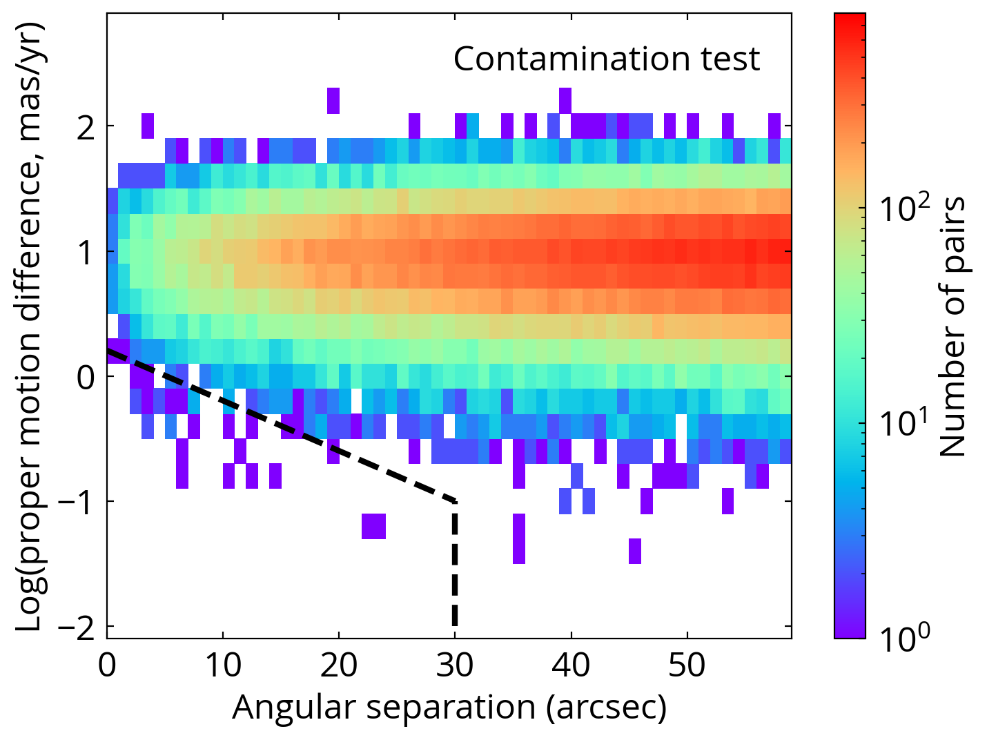
To better quantify the contamination from the chance-alignment pairs, we conduct a test by offsetting the H3 targets’ Galactic latitudes by 1 degree (1 degree corresponds to 17 pc at a distance of 1 kpc) to the North (with the coordinates of field Gaia stars unshifted) and redo the wide binary search (Lépine & Bongiorno, 2007). Therefore, all the pairs from this test are chance-alignment pairs. The result is shown in Fig. 1, middle panel. This contamination test well reproduces the chance-alignment pairs in the left panel, except that the left panel has an additional wide binary population at small angular separations and small proper motion differences.
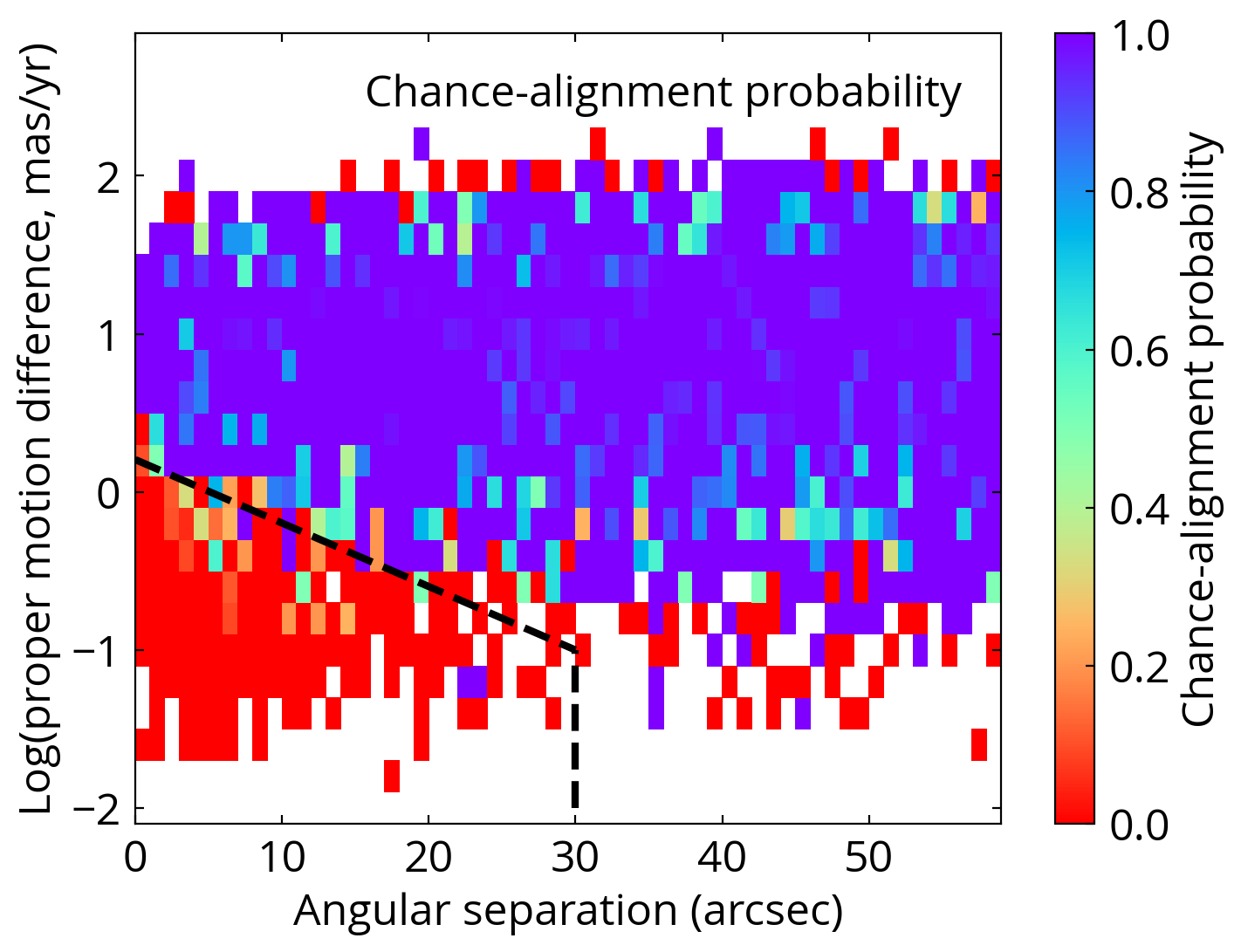
In the right panel of Fig. 1, we compute the chance alignment probability (CAP) in each two-dimensional bin. Specifically, CAP in every bin is calculated by the number of pairs in the middle panel divided by the number of pairs in the left panel. The right panel of Fig. 1 shows that the wide binaries can be selected by small proper motion differences with CAP less than 10% out to 30 arcsec. At separations arcsec, CAP is still less than % at small proper motion differences ( mas yr-1), indicative of the existence of wide binaries beyond 30 arcsec ( pc for stars at 1 kpc distances), consistent with the simulation and observation that a significant fraction of comoving stars with separations up to pc are conatal (Kamdar et al., 2019; Nelson et al., 2021). Some low CAP pixels at the edge of large proper motion differences are due to small-number statistics.
In this paper, we focus on the wide binaries with angular separations arcsec for their larger sample size and the lower CAP. We adopt an empirical demarcation line (the dashed lines in Fig. 1) to select high-confidence wide binaries with CAP%. The demarcation line starts from mas yr-1 at 0″ separation to mas yr-1 at 30″, connected by a straight line in the log-linear space. Pairs below this demarcation line and at angular separations arcsec are selected as wide binaries, resulting in 800 wide binaries and 2 resolved triples. There are 33 pairs located below this demarcation line in the contamination test in the middle panel of Fig. 1, suggesting that the contamination rate from the chance-alignment pairs in our wide binary sample is per cent. A more stringent selection (e.g. angular separations arcsec instead of arcsec) does not change our main results and conclusions.
We provide an electronic catalog for the H3 wide binaries. Table 1 presents the data model for the catalog. Field names starting with the prefix ‘0_’ are the information for the H3 stars, and those starting with the prefix ‘1_’ are for the companions. A resolved triple system would have two entries in the table with the same H3 star and different companion stars.
| Field | Description |
| 0_source_id | Gaia EDR3 source_id of the H3 star |
| 0_ra | Right ascension of the H3 star from Gaia EDR3 (J2016.0; deg) |
| 0_dec | Declination of the H3 star from Gaia EDR3 (J2016.0; deg) |
| 0_parallax | Parallax of the H3 star from Gaia EDR3 (mas) |
| 0_parallax_error | Uncertainty in 0_parallax from Gaia EDR3 (mas) |
| 0_pmra | Proper motion in right ascension direction of the H3 star from Gaia EDR3 (mas yr-1) |
| 0_pmra_error | Uncertainty in 0_pmra (mas yr-1) from Gaia EDR3 |
| 0_pmdec | Proper motion in declination direction of the H3 star from Gaia EDR3 (mas yr-1) |
| 0_pmdec_error | Uncertainty in 0_pmdec (mas yr-1) from Gaia EDR3 |
| 0_G | Apparent G-band magnitude of the H3 star from Gaia EDR3 (mag) |
| 0_H3_ID | H3 id for the H3 star |
| 0_FeH | Iron abundance [Fe/H] of the H3 star measured by H3 (dex) |
| 0_aFe | -captured elemental abundance [/Fe] of the H3 star measured by H3 (dex) |
| 0_Teff | Effective temperature of the H3 star measured by H3 (K) |
| 0_logg | Surface gravity of the H3 star measured by H3 ( cgs) |
| 0_Vrad | Radial velocity of the H3 star measured by H3 ( km s-1) |
| 0_dist_adpt | Heliocentric distances of the H3 star measured by H3 (kpc) |
| 0_Etot | Total orbital energy of the H3 star ( km2 s-2) |
| 0_Etot_err | Uncertainty in 0_Etot ( km2 s-2) |
| 0_Lz | Orbital momentum along the Galactic z-axis of the H3 star ( kpc km s-1) |
| 0_Lz_err | Uncertainty in 0_Lz ( kpc km s-1) |
| 1_source_id | Gaia EDR3 source_id of the companion star |
| 1_ra | Right ascension of the companion star from Gaia EDR3 (J2016.0; deg) |
| 1_dec | Declination of the companion star from Gaia EDR3 (J2016.0; deg) |
| 1_parallax | Parallax of the companion star from Gaia EDR3 (mas) |
| 1_parallax_error | Uncertainty in 1_parallax from Gaia EDR3 (mas) |
| 1_pmra | Proper motion in right ascension direction of the companion star from Gaia EDR3 (mas yr-1) |
| 1_pmra_error | Uncertainty in 1_pmra (mas yr-1) from Gaia EDR3 |
| 1_pmdec | Proper motion in declination direction of the companion star from Gaia EDR3 (mas yr-1) |
| 1_pmdec_error | Uncertainty in 1_pmdec (mas yr-1) from Gaia EDR3 |
| 1_G | Apparent G-band magnitude of the companion star from Gaia EDR3 (mag) |
| separation_arcsec | Angular separation of the wide binary (arcsec) |
| separation_AU | Projected physical separation of the wide binary (AU) |
| pm_diff | Proper motion difference of the wide binary ( mas yr-1) |
| triple | 1 if it is a resolved triple, otherwise 0 |
| halo_disk | 1 if it is in the halo; 0 if it is in the disk; if it does not pass the kinematic criteria |
4 Properties of H3 wide binaries
4.1 Distances and binary separations
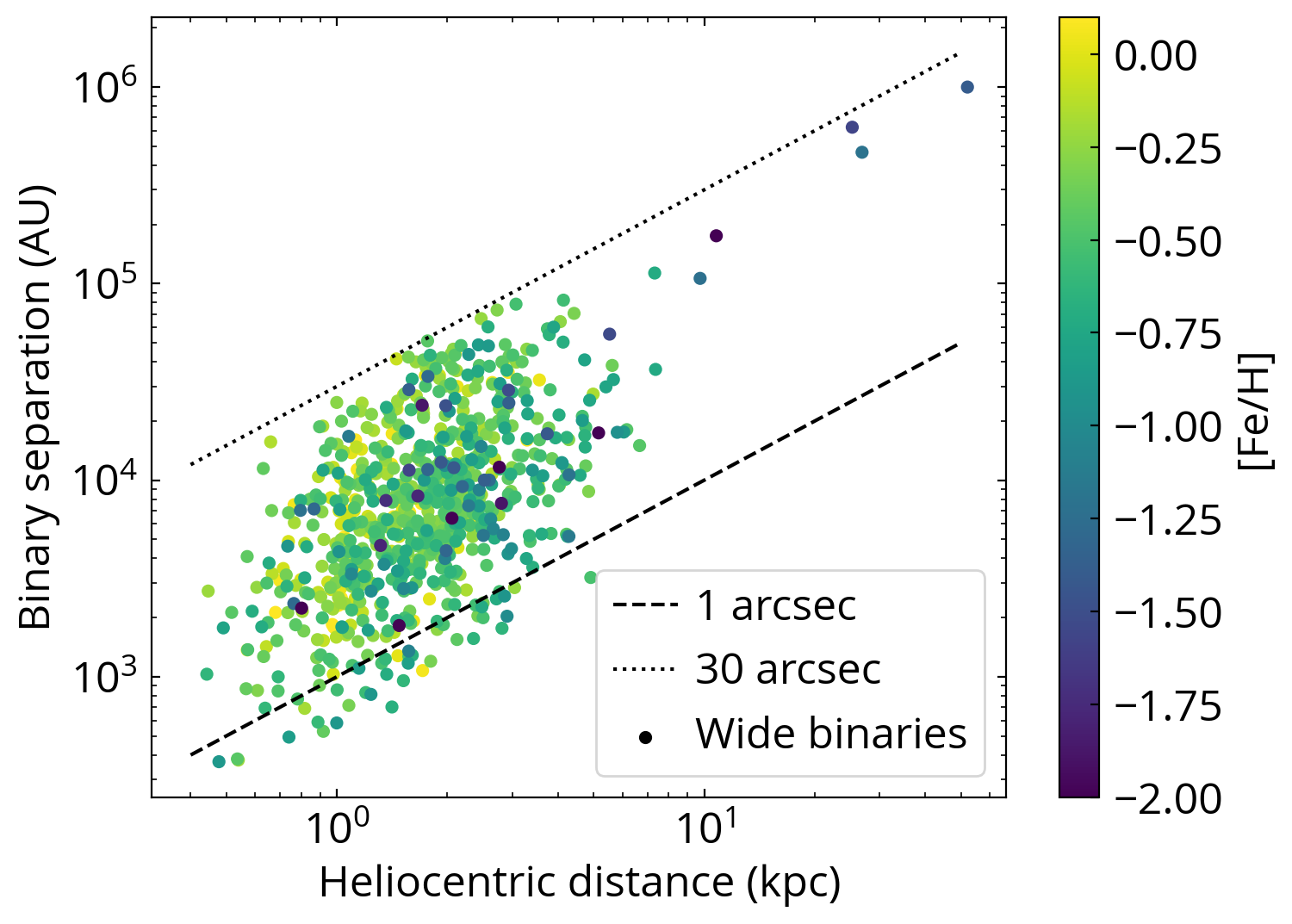
Fig. 2 shows the binary separations and heliocentric distances of the wide binaries, color-coded by their iron abundances. Most of the wide binaries have angular separations between 1 (dashed line) and 30 arcsec (dotted line), where the former is close to Gaia’s spatial resolution and the latter is due to our selection criterion. Most of these wide binaries are located 1-5 kpc from the Sun. Those closer to the observer tend to have higher iron abundances.
There are four wide binaries located at larger than 10 kpc from the Sun, with the farthest one at 50 kpc. They all have very wide binary separations of pc. These distant wide binaries are valuable for probing the gravitational interactions in the outer Milky Way. Even though these distant wide binaries may suffer from a higher chance-alignment probability because of their larger angular separations ( arcsec) and smaller total proper motions ( mas yr-1), their companions’ photometry, as shown in the next Section, are consistent with their H3 stars’ isochrones, suggesting that they are not chance-alignment pairs. One possibility is that they are pairs with other member stars in a yet unidentified stream, instead of being a wide binary. This may explain why these four distant wide binaries all have large angular separations. Further work is needed to investigate if they are wide binaries or stream-member pairs.
4.2 Hertzsprung-Russell diagram
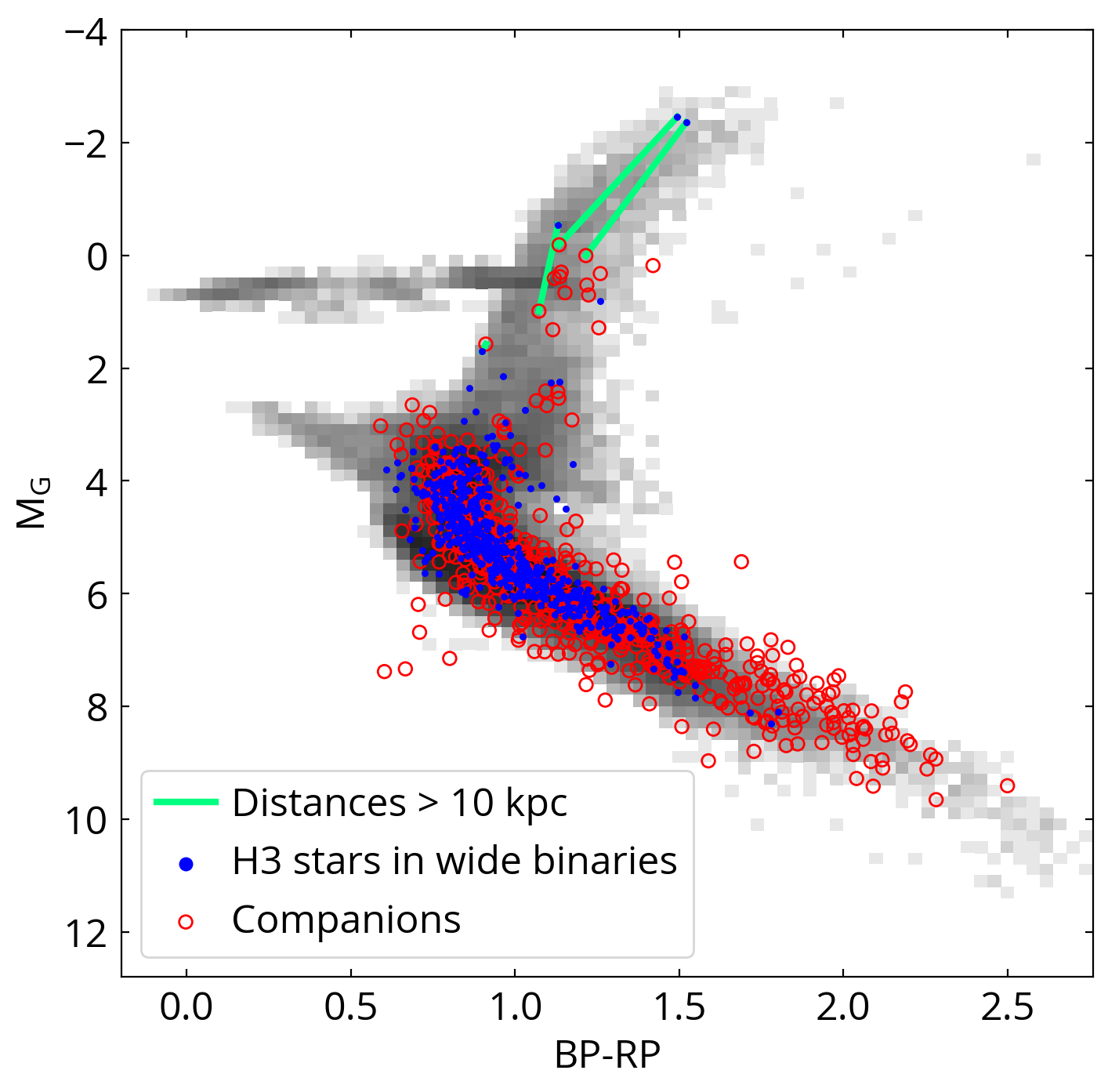
Fig. 3 shows the Hertzsprung-Russell (H-R) diagram of the wide binaries, where the absolute G-band magnitudes are computed using the distances measured from MINESweeper. The non-H3 stars adopt the same distances as their H3 companions. We apply the criteria on BP and RP as described in Sec. 2.2 for more robust photometry, resulting in 584 pairs. The gray background shows the distribution of all stars in the H3 catalog, where most of them do not have wide companions. Most of the wide binaries identified here are main-sequence stars, and some are located on the giant branch. The companions scatter more around the main sequence track because they are fainter and more likely to have larger uncertainties in their photometry.
The solid green lines in Fig. 3 highlight the four wide binaries with distances kpc. They are rare double-giant wide binaries due to the selection effect that we only see giant stars at large distances. One of them has nearly the same G and BP-RP magnitudes for the two member stars, forming an unusual twin giant binary where two stars have nearly identical evolutionary stages. Fig. 3 shows that the non-H3 companions of these distant wide binaries have Gaia photometry consistent with the H3 stars’ isochrones, suggesting that they are not chance-alignment pairs.
Because there are limited regions in the H-R diagram where stars can exist, the locations of the non-H3 companions in the H-R diagram are a useful diagnostic of whether they are genuine binary companions. Since wide binaries with separations a few pc are conatal, two stars of the same wide binary have nearly identical stellar ages and chemical abundances (Andrews et al., 2018; Kamdar et al., 2019; Hawkins et al., 2020; Nelson et al., 2021). We use the distance, [Fe/H]init, and [/Fe]init measured from the H3 stars to investigate whether the companion stars are located close to the corresponding MIST isochrone in the H-R diagram. We define color deviation BP-RP by:
| (2) |
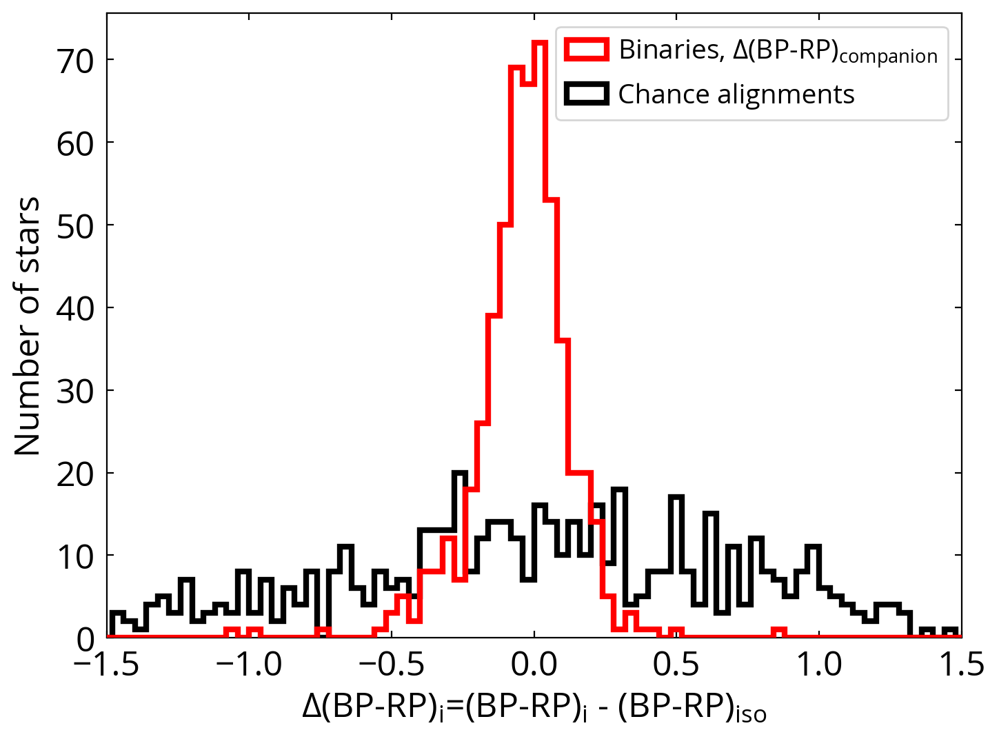
where is the observed Gaia BP-RP color for star (a non-H3 companion), and is the expected BP-RP color from the MIST isochrone for this star given its absolute G-band magnitude. If the companion star is located close to the expected isochrone, then . We use brutus111https://github.com/joshspeagle/brutus (Speagle et al. submitted) to interpolate the MIST v2.0 grid (Choi et al., 2016) given the [Fe/H]init, [/Fe]init, stellar age, and measured from the H3 star. Then for a non-H3 companion, its expected color is computed from the MIST isochrone given its absolute G-band magnitude, where we assume that the non-H3 companion has the same distance as the H3 star. This step also requires that an absolute G-band magnitude only maps to a single BP-RP value, which is satisfied for the main-sequence phase and the early stage of the giant phase. For the late giant phase, one absolute G-band magnitude can intersect an isochrone at multiple BP-RP colors. Therefore, we only compute for stars where their can be uniquely determined, resulting in 546 pairs. Because brutus includes the extinction when computing , the resulting is extinction corrected.
Fig. 4 shows the distribution of for the non-H3 members of the wide binaries, , and chance-alignment stars, . The chance-alignment stars are selected by large proper motion differences mas yr-1 and within 10 arcsec around the H3 stars. The (red histogram) is clustered around 0, indicating that these companions are located close to the expected isochrone. The width of is mainly due to the uncertainties of distance estimates and photometry. For comparison, chance-alignment companions (black histogram) have a broad distribution of . This is because these chance-alignment stars in general have different distances as the H3 stars, resulting in non-zero due to their erroneous absolute G-band magnitudes when we assume they have the same distances as the H3 stars. Therefore, Fig. 4 suggests that the majority of the wide binary candidates are indeed genuine wide binaries instead of chance-alignment stars.
4.3 Galactic kinematics
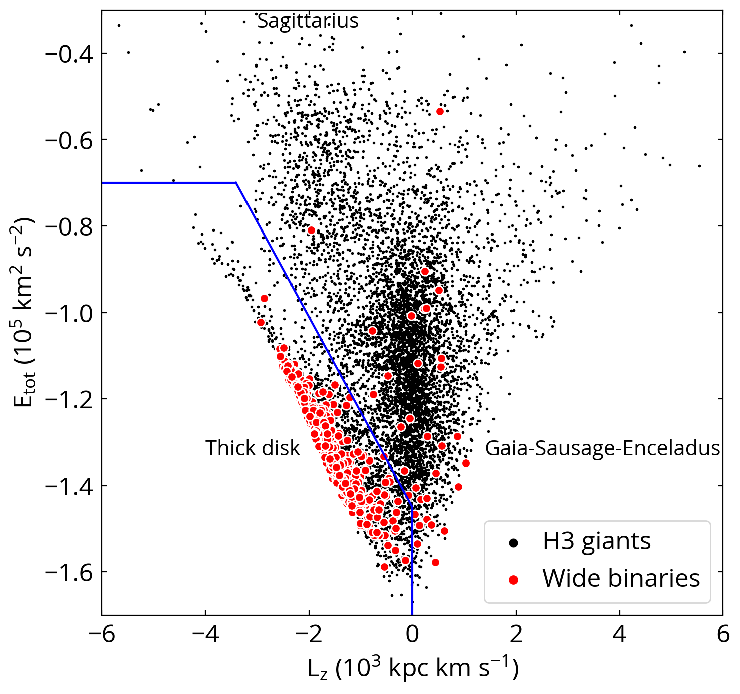
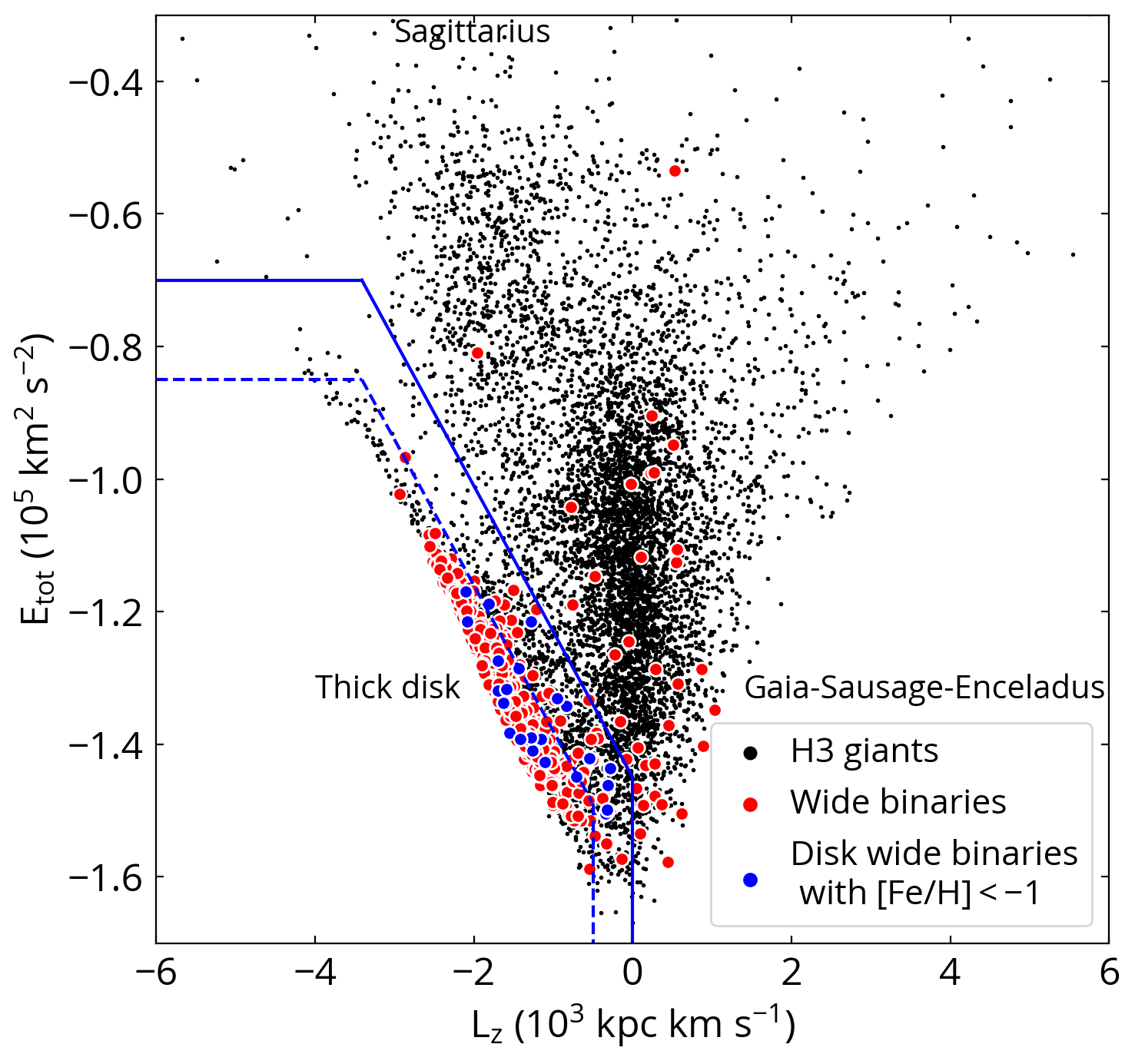
Galactic kinematics is key to revealing substructures in the Milky Way’s stellar halo (Johnston et al., 1996; Helmi & White, 1999; Bullock & Johnston, 2005; Cooper et al., 2010). Fig. 5 shows the H3 giants (black points) and the wide binaries (red points) in the - space. We select H3 giants (black points) by and adopt the same criteria in Sec. 2.1 and Sec. 2.3 to ensure reliable kinematic measurements, except that we include giant stars from the Sagittarius (Sgr_FLAG==1). Applying our wide binary search to stars with Sgr_FLAG==1 results in two additional wide binaries, but both of them do not satisfy the kinematics criterion in Sec. 2.3, making no change to Fig. 5. The distance distributions vary in the - space. In particular, the thick disk stars are on average closer to the Sun than the halo stars. Using the H3 giants yields a relatively unbiased view with respect to the distances of the substructures in the halo out to kpc (Naidu et al., 2020).
Two main structures in Fig. 5 are the thick disk and the Gaia-Sausage-Enceladus (the overdensity centered at ) remnant. There are more other substructures related to previous accretion events in the halo detailed in Naidu et al. (2020). These substructures mark the rich accretion history of the Milky Way. In particular, Gaia-Sausage-Enceladus is from a merger event with a mass ratio of 1:4 about 10 Gyr ago (Belokurov et al., 2018; Helmi et al., 2018; Bonaca et al., 2020; Koppelman et al., 2020; Naidu et al., 2021), accounting for % of the halo population within 20 kpc of the inner Milky Way (Naidu et al., 2020). The merger of Gaia-Sausage-Enceladus likely dynamically heated up the Milky Way’s disk and formed the thick disk (Gallart et al., 2019). Then the Sagittarius dwarf galaxy started infalling around 8 Gyr ago with a mass ratio of % (Ibata et al., 1994; Law et al., 2010; Dierickx & Loeb, 2017; Fardal et al., 2019). Since then, the Milky Way has undergone a relatively quiescent evolution and grown the low- (thin) disk (Wyse, 2001, 2009; Ting & Rix, 2019; Bonaca et al., 2020).
In Fig. 5, we show all 798 wide binaries that pass the kinematics quality criteria. We use the - plane to separate the halo and the thick-disk populations. Due to H3’s target selection, 90% of the H3 stars have Galactic heights kpc, and therefore we refer to the disk stars in the H3 as thick-disk stars. The solid blue line in Fig. 5 is our empirical demarcation line, with thick disk stars located in the lower-left part and the halo stars for the rest. The disk-star selection is: (1) km2 s-2; (2) ; (3) , where ( km2 s-2) ( kpc km s-1), and is the Boolean ‘and’ operator. With this selection, we have 763 (96%) thick-disk wide binaries and 33 (4%) halo wide binaries. If we apply this disk-halo selection to the entire H3 catalog with the same quality criteria, 16% of the H3 stars are classified as halo stars. One main reason for the lower efficiency of identifying wide binaries in the halo than in the disk is that halo stars are more distant, making Gaia more difficult to resolve or to detect the companion. The other reason is their different wide binary fractions, which will be detailed in the next Section.
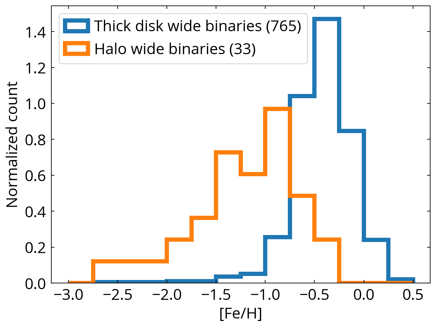
Fig. 6 shows the normalized distribution of surface iron abundances for disk and halo wide binaries. Halo wide binaries have [Fe/H] peaking around , similar to the metallicity of Gaia-Sausage-Enceladus remnant (Naidu et al., 2020). Wide binaries in the thick disk have [Fe/H] centering around . Both resolved triples belong to the disk with a relatively high [Fe/H] of and . The most metal-poor wide binaries in our sample are [Fe/H] in the disk and [Fe/H] in the halo (the distant giant twin in Fig. 3), among the most metal-poor wide binaries known today (Reggiani & Meléndez, 2018; Hwang et al., 2021; Lim et al., 2021).
It is particularly interesting that many halo wide binaries have and associated with the Gaia-Sausage-Enceladus remnant. The stars from the Gaia-Sausage-Enceladus are characterized by their high Galactic eccentricities (Belokurov et al., 2018; Naidu et al., 2020). Indeed, 26 out of the 33 halo wide binaries have , suggesting that they are from the Gaia-Sausage-Enceladus remnant. The rest of 7 low-eccentricity () halo wide binaries may belong to the in-situ halo, and 3 of them have [Fe/H] and [/Fe] satisfying the criteria of the in-situ halo in Naidu et al. (2020). Together with a recent finding of a wide binary associated with the Sequoia remnant (Lim et al., 2021), our results unambiguously show the existence of wide binaries among the accreted stars.
The two halo wide binaries having the largest in Fig. 5 are the ones with distances kpc discussed earlier in Sec. 4.1 and 4.2. The one with the largest has a highly eccentric Galactic orbit () and may be considered as Gaia-Sausage-Enceladus’ member in Naidu et al. (2020), despite of its unusually high . The other one has a modest Galactic eccentricity of 0.47 does not belong to the Gaia-Sausage-Enceladus. Its kinematics is similar to the Sagittarius in - space, but its and do not fall in the selection for Sagittarius stars in Johnson et al. (2020).
There are three metal-poor wide binaries with [Fe/H] in the disk. All of them are main-sequence stars with ages Gyr according to the MINESweeper spectroscopic-photometric estimates, high [/Fe] (0.56, 0.54, 0.37), and prograde orbits (). Although the sample is limited, they may be related to the ancient Milky Way disk (Carter et al., 2021).
5 The abundance dependence of the wide binary fraction
5.1 Bayesian formulation
Our purposes are twofold: we aim to (1) compare the halo and disk wide binary fraction at a fixed metallicity, and to (2) investigate the metallicity trend of the disk wide binary fraction. Due to the small sample size and the limited metallicity range, we are not able to investigate the metallicity dependence of the wide binary fraction within the halo sample. These investigations need to take distances and masses into account. At a fixed binary separation, it is more difficult to spatially resolve more distant binaries, and companions of more distant binaries are more likely to fall below the magnitude limit of Gaia. Furthermore, because H3 selects targets based on apparent magnitudes, different metallicity and mass ranges are probed at different distances. Therefore, to compare wide binary fractions at different metallicities, we need to include the distance and mass dependence in the model.
For an H3 star , we model the probability that this star has a wide binary companion detected by Gaia by
| (3) |
where is a Boolean value indicating if the star is a wide binary () or not () in our sample, and and are the mass and the distance of the star in units of solar mass and kpc. The probability that a star does not have a resolved Gaia companion is . is the set of the model parameters including the exponents and and other parameters involved in which will be introduced shortly. We adopt a power-law form for the mass and distance dependence, with exponents and . The distance dependence comes from the selection efficiency due to the angular resolution and the magnitude limit, and their relation depends on the underlying binary separation distribution. We run a simulation for wide binaries with companions following the Kroupa initial mass function (Kroupa, 2001) from 0.2 to 1 M⊙ and a power-law binary separation distribution from to AU. The mass is then converted to the absolute -band magnitude using the MIST isochrone with an assumption that they are main-sequence stars. Adopting an angular resolution of 0.5″ and a -band magnitude limit of 20 mag, the simulation finds that a power-law form is a robust description ( for this particular case) for the distance dependence of the detection fraction at distances between 0.5 to 5 kpc.
in Eq. 3 is the wide binary fraction at different chemical abundances for star . We assume that the [Fe/H] and [/Fe] dependences are independent and therefore the function is separable:
| (4) |
To investigate the different iron abundance dependence between halo and disk stars, we define as
| (5) |
We use a single value for the halo sample because of its small sample size and limited abundance range. For disk stars, we consider a multi-step function such that if . Based on the sample size, the metallicity bin is chosen to be [, , , , 0, 0.5]. In this way, we can measure the disk wide binary fraction in each metallicity bin.
The dependence on the -captured abundance is encoded in in Eq. 4 by
| (6) |
where is the only free parameter for the slope of the dependence on [/Fe], and means no dependence on [/Fe]. Because [Fe/H] is the main focus here, we choose a simpler form for [/Fe] than [Fe/H] to reduce the number of free parameters involved, and we use the same [/Fe] relation for both disk and halo stars.
Therefore, in Eq. 3 includes 9 free parameters: and for the mass and distance dependence, for the [/Fe] dependence (Eq. 6), one from , and 5 from . We do not marginalize the uncertainties of stellar parameters ([Fe/H]i, etc.) because their uncertainties from H3 are small and do not significantly affect the results.
in Eq. 3 can be understood as the observed fraction of binaries with separations of about - AU in the H3 data anchored at 1 M⊙ stars at a distance of 1 kpc from the Sun. In other words, for a 1 M⊙ star (=1) at a distance of 1 kpc (=1), the probability of this star having an observed wide companion is , depending on whether it is a disk or halo star and its iron and -captured abundances (Eq. 4-6). For stars with arbitrary masses () and distances (), the probability of having an observed companion () depends on the wide binary fraction and the distance and mass dependence controlled by the power-law indices and (Eq. 3).
The Bayesian formulation is
| (7) |
where is the posterior distribution of the parameter set given , the observed wide binary identification for the H3 sample. We use uninformative flat priors for and exclude the parameter space that makes the probability for any in Eq. 3. Eq. 7 can be rewritten as
| (8) |
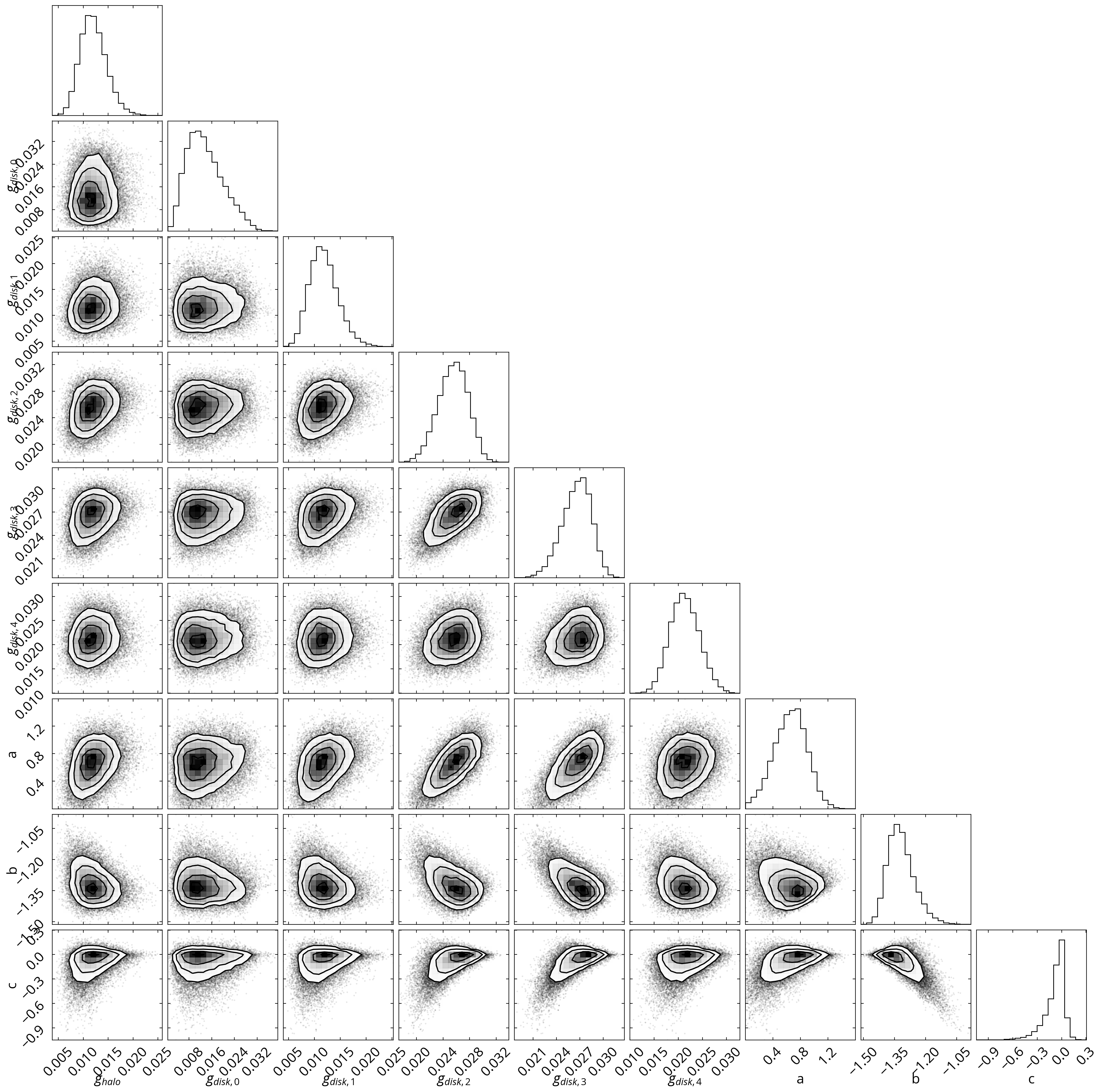
where is from Eq. 3. We use emcee (Foreman-Mackey et al., 2013), an affine-invariant ensemble sampler for Markov chain Monte Carlo, to sample the posteriors of Eq. 8. To distinguish halo and disk stars, we require the sample to have good Galactic kinematics with criteria described in Sec. 2.3. We limit the sample to heliocentric distances kpc because wide binary detectability beyond this distance is low and may not follow the power-law distance dependence we adopt. Two resolved triples are excluded from this analysis. Therefore, this analysis has 8610 halo stars (23 halo wide binaries) and 80572 disk stars (757 disk wide binaries). The resulting corner plot (the two-dimensional posterior distribution) made using corner (Foreman-Mackey, 2016) is shown in the Appendix, Fig. 1.
Our formulation includes the mass and distance dependence of binary detectability in Eq. 3. This is important because halo and disk stars have different distance and mass distributions due to their physical differences and H3’s target selection. This formulation assumes that the wide binary fractions of all stars follow the same mass, distance, and [/Fe] dependence. This implicitly assumes that the mass-ratio distribution is not a strong function of metallicities and binary separations. This mass-ratio assumption is validated by Moe & Di Stefano (2017) that the mass-ratio distribution for binaries at AU is consistent with random pairings from the initial mass function. In addition, we assume that the [Fe/H] and [/Fe] are independent and therefore are separable in Eq. 4. Future studies are needed to investigate these assumptions.
5.2 Wide binary fraction in the halo and the disk, and its metallicity dependence
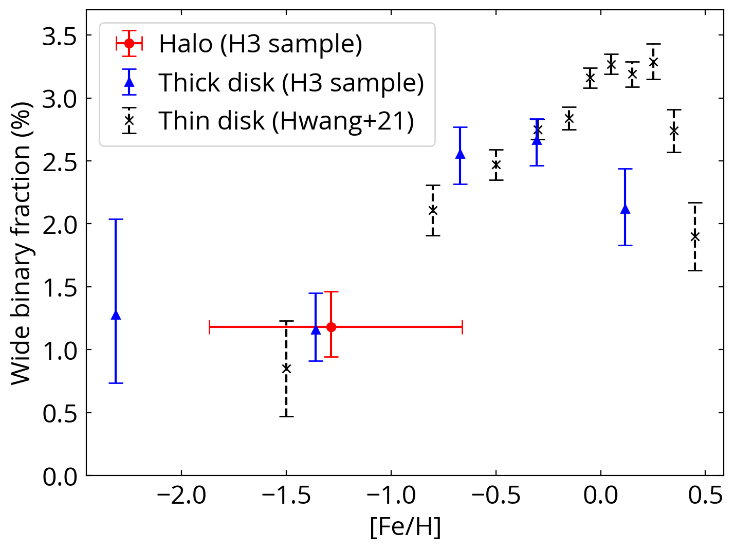
Fig. 7 shows the wide binary fraction as a function of [Fe/H]. The red circle and blue triangles show the measurements for the halo and the thick disk, respectively. Their [Fe/H] values are the mean metallicities in each sample, and the horizontal error bar of the halo sample indicates the 16-84 percentiles of its metallicity distribution. Their wide binary fractions are and ([Fe/H]) in Eq. 4, defined as the observed values at 1 kpc for 1 M⊙ stars. The wide binary fractions and their errors in Fig. 7 are the 16-50-84 percentiles of their marginalized distributions.
For comparison, in Fig. 7 we overplot the results from Hwang et al. (2021) as black crosses where the 500-pc sample is dominated by the thin-disk stars and the wide binaries refer to separations between and AU, with [Fe/H] values indicating the centers of the bins. The wide binary fractions of the disk and halo stars from this work (red circle and blue triangles) can be compared with each other in the absolute sense, meaning that the halo wide binary fraction is consistent with that in the thick disk at a fixed [Fe/H], taking into account the differences in the distance and mass distributions. Although the thick-disk wide binary fractions from this work and those from Hwang et al. (2021) happen to have similar values in Fig. 7, they should only be compared in a relative sense (i.e. the overall metallicity trend) but not in an absolute sense, because they use samples that have different detection limits for the companions due to the different distance, binary separation, and mass ranges.
Fig. 7 shows that the wide binary fraction in the thick disk decreases towards the low-metallicity end. This is similar to the trend in the thin disk (Hwang et al., 2021), but now this work extends the trend down to [Fe/H]. At [Fe/H], the H3 sample shows a flat relation between the wide binary fraction and the metallicity, in contrast to the peak at [F/H] for the thin-disk stars. This is consistent with Hwang et al. (2021) where we found that the peak at [F/H] is more prominent for younger disk stars.
Hwang et al. (2021) differentiated the thick-disk stars and halo stars using total 3-dimensional velocities and the maximum Galactic heights of the stellar orbits. We found that at a fixed metallicity, the wide binary fraction of the halo seems consistent with that of the thick disk. However, there are only two halo wide binary candidates in Hwang et al. (2021), so the conclusion is still limited by small number statistics.
Here with a better Galactic kinematics selection and a larger halo wide binary sample from the H3 survey, we robustly show that the wide binary fraction of the halo stars is consistent with that of the thick-disk stars at a fixed metallicity. This result suggests that iron abundance is the main driver of the wide binary fraction, and that the thick disk and halo stars do not have significantly different wide binary fractions once the metallicity, distance, and mass are taken into account.
The [/Fe] dependence is an important clue about binary formation. Mazzola et al. (2020) find that the close binary (10 AU) fraction anti-correlates with [/Fe]. This relationship may arise because the dust formed from -captured elements affects the fragmentation of the protostellar disks by changing its opacity. In contrast, Niu et al. (2021) consider the total binary fraction and suggest a tentative positive correlation between the binary fraction and [/Fe] at a fixed [Fe/H].
In contrast to the previous studies, here we investigate the [/Fe] dependence of the wide binary fraction at separations AU. The parameter for the [/Fe] dependence in Eq. 6 is measured to be , where the errors correspond to 16-84 percentiles. Therefore, is consistent with zero and the wide binary fraction does not appear to depend on the -captured abundances. The different [/Fe] dependence of the close and wide binary fraction suggests that different formation mechanisms are responsible for close and wide binaries, similar to the conclusions from the [Fe/H] dependence (El-Badry & Rix, 2019; Hwang et al., 2021).
One concern is whether the metal-poor disk stars at [Fe/H] are contaminated by halo stars, which might explain the similar wide binary fractions in the halo and the thick disk at [Fe/H]. Fig. 8 shows the disk wide binaries with [Fe/H] (blue points) in the - space. There is no strong tendency for metal-poor wide binaries being located close to the original demarcation line (solid blue line). While some wide binaries are closer to the demarcation line, they may still be genuine metal-poor disk stars because the metal-weak thick disk is located at a similar - region (Naidu et al., 2020). To test how the disk-star selection affects the result, we use a more strict disk-star selection (dashed line in Fig. 8): (1) ; (2) ; (3) . Using this more strict disk-star selection and the same Bayesian approach from Sec. 5.1, we obtain wide binary fractions of the thick disk consistent with Fig. 7. Therefore, the contamination of halo stars in the disk selection plays a minor role in our results.
6 Discussion
6.1 Comparison with the literature
In the pre-Gaia era when high-precision parallaxes were not available for most of the stars, the reduced proper motion diagram was used to distinguish high-velocity halo stars from lower-velocity disk stars and to identify halo wide binaries. The reduced proper motion diagram uses proper motions as a proxy for distances because closer stars have larger proper motions, and halo stars are more separated from the disk stars because of halo stars’ lower metallicities and higher spatial velocities (Salim & Gould, 2002). Using this method, previous studies have found 100-200 halo(-like) wide binary candidates (Chaname & Gould, 2004; Quinn & Smith, 2009; Allen & Monroy-Rodríguez, 2014; Coronado et al., 2018). Wide binaries in the halo can be used to constrain the mass of massive compact halo objects – for example, the contribution of free-floating black holes and neutron stars to the mass budget of the Universe (Yoo et al., 2004; Quinn et al., 2009; Monroy-Rodríguez & Allen, 2014).
In addition to proper motions, the reduced proper motion diagram uses photometry to distinguish halo and disk stars. However, because lower-metallicity stars have a higher close binary fraction (Moe et al., 2019), and close binaries are more likely to have wide companions (Hwang et al., 2020), metal-poor stars selected from the reduced proper motion diagram may have binary-related selection effects because unresolved companions make the systems deviate from the reduced proper motion diagram.
Gaia provides high-precision astrometry for billions of stars (Gaia Collaboration et al., 2016), making the search for a large number of wide binaries possible (Oh et al., 2017; El-Badry & Rix, 2018; Jiménez-Esteban et al., 2019; Hartman & Lépine, 2020). Using Gaia EDR3, El-Badry et al. (2021) have cataloged about a million wide binaries within 1 kpc. By cross-matching this catalog the with LAMOST survey DR6 (Deng et al., 2012; Zhao et al., 2012) and using LAMOST’s radial velocities to compute and , we find about 50 halo wide binaries that satisfy the halo selection from Sec. 4.3 and SNR in g-band from LAMOST with a lower spectral resolution () than H3.
Our wide binaries feature the most distant ( kpc and four candidates at kpc), most metal-poor (down to [Fe/H]) sample with detailed abundance and kinematic measurements from a spectroscopy. The H3 survey is critical in providing a homogeneous sample of disk and halo stars to compare the wide binary fractions among various subsamples. Since our wide binary search depends only on astrometry and not on photometry, our selections are less affected by unresolved companions. Our halo classifications and the association with Gaia-Sausage-Enceladus remnant are robust thanks to the precise and measurements from H3.
6.2 Origin of the iron-abundance dependence
Hwang et al. (2021) identified 7671 wide binaries within 500 pc with projected separations between and AU. These wide binaries are mostly thin- and thick-disk stars. With the iron abundances measured from LAMOST (Wu et al., 2011a, b; Ting et al., 2019; Xiang et al., 2019), we found that the wide binary fraction at - AU peaks at around [Fe/H], and decreases towards both low and high metallicity ends (black symbols in Fig. 7).
Hwang et al. (2021) proposed several possibilities to explain such metallicity dependence. The positive correlation between [Fe/H] and the wide binary fraction at [Fe/H] may be due to the denser formation environments in the earlier Universe that tend to disrupt the wide binaries. At [Fe/H], the anti-correlation between [Fe/H] and the wide binary fraction may be due to some wide binaries forming from the dynamical unfolding of compact triples (Reipurth & Mikkola, 2012; Elliott & Bayo, 2016), and thus they inherit the metallicity dependence from the close binary fraction (Raghavan et al., 2010; Yuan et al., 2015; Badenes et al., 2018; Moe et al., 2019; El-Badry & Rix, 2019). The radial migration of Galactic orbits (Sellwood & Binney, 2002) may cause such non-monotonic metallicity dependence, either due to different formation environments at different galactocentric radii or due to disruption of wide binaries during the enhanced interaction with high-density gas clumps during the migration process. Wide binary disruptions by passing stars are unlikely to play an important role because the disruption timescale of Gyr for AU binaries is too long (Weinberg et al., 1987).
If the metallicity dependence of the wide binary fraction is due to the radial migration, which is more important for disk stars, we would expect a higher wide binary fraction in the halo than in the disk. Our H3 results suggest that iron abundance is the main driver for the wide binary fraction (Fig. 7), instead of their origin (disk versus halo) nor -captured abundance. The similar wide binary fractions in the halo and the disk implies that radial migration is not the main cause for the metallicity dependence of the wide binary fraction at [Fe/H].
Our leading explanation for the iron abundance dependence of the wide binary fraction at [Fe/H] is that the formation environments are denser at lower [Fe/H], which are more disruptive for wide binaries. In particular, studies have found that the star formation environments have higher pressures and densities at higher redshifts, and higher-mass clusters tend to form in such environments (Harris & Pudritz, 1994; Elmegreen & Efremov, 1997; Kravtsov & Gnedin, 2005; Kruijssen, 2014; Ma et al., 2020). Therefore, the lower wide binary fraction may reflect their denser formation environments in the earlier epochs.
Although a lower-metallicity population is on average older than a higher-metallicity sample (Casagrande et al., 2011; Bensby et al., 2014; Silva Aguirre et al., 2018), our result is better explained by the metallicity dependence instead of the age dependence. Following Bonaca et al. (2020), we select main-sequence turn-off stars by and SNR for their precise age measurements. This sample shows that, for our H3 thick-disk sample, the mean stellar age changes approximately linearly from Gyr at [Fe/H] dex (Carter et al., 2021) to Gyr at [Fe/H] dex. This does not explain the metallicity trend in Fig. 7 where the wide binary fraction becomes flat at [Fe/H] when the mean age changes by about 2 Gyr from [Fe/H] to [Fe/H]. Therefore, our results suggest that stellar ages play a minor role.
While halo wide binaries are currently not susceptible to disruptions via radial migration and giant molecular cloud, they were once in presumably gas-rich environments in the progenitor (dwarf) galaxies. It is intriguing that halo and thick-disk wide binary fractions are similar at a fixed metallicity despite their potentially different formation environments. The similar wide binary fractions between the thick disk and the halo may hint that the metallicity and the formation environment properties are tightly correlated, and by controlling the metallicity, we mitigate the differences in their formation environments. One important formation environment property is the cluster mass function because wide binaries are sensitive to the density (which correlates with mass) of clusters (e.g. Parker et al. 2009; Geller et al. 2019). Therefore, one possibility is that the Milky Way and the Gaia-Sausage-Enceladus dwarf may have similar cluster mass functions at a fixed metallicity (Krumholz et al. 2019), resulting in the similar wide binary fractions.
Since wide binaries are unlikely to survive in globular clusters (e.g. Ivanova et al. 2005), our results can place a rough constraint on the contribution of disrupted globular clusters to the stellar halo. Here we find that the wide binary fraction of the halo is consistent with that of the thick disk (Fig. 7). Assuming that the original halo wide binary fraction (halo stars that are not from disrupted globular clusters) is the same as that in the disk at a fixed metallicity and that the wide binary fraction from disrupted globular clusters is zero, our result implies that the disrupted globular clusters contribute less than % of the halo. If the disrupted globular clusters contribute more than % of the halo, the halo wide binary fraction would be significantly lower than that of the thick disk, inconsistent with our results. The % constraint is consistent with other studies finding that % of halo stars originate in disrupted globular clusters (Martell & Grebel, 2010; Martell et al., 2011, 2016; Koch et al., 2019), or likely an even smaller fraction (Naidu et al., 2020). Our constraint serves as a useful independent check but is likely tentative because of the various assumptions used, and it may be possible that wide binaries can form during globular cluster disruption (Peñarrubia, 2021).
7 Conclusions
What determines the wide binary fraction remains not well understood. Hwang et al. (2021) found that the wide binary fraction of disk stars peaks around solar metallicity ([Fe/H]) and decreases toward both low and high metallicity end. We proposed three possible scenarios that may explain this metallicity dependence, including the radial migration of Galactic orbits. In this paper, armed with the thick-disk and halo wide binaries identified from the H3 survey, we rule out the radial migration scenario at [Fe/H]. Our findings include:
-
1.
With Gaia’s astrometry, we search for resolved wide companions around the H3 stars (Fig. 1). Our search results in a total of 800 wide binaries and two resolved triples. The photometry of the non-H3 companions are consistent with the isochrones of the H3 stars, suggesting that most of them are genuine wide binaries instead of chance-alignment pairs (Fig. 4).
-
2.
Most of the wide binaries are main-sequence stars (Fig. 3), with binary separations ranging from to AU and heliocentric distances kpc (Fig. 2). These wide binaries have [Fe/H] down to (Fig. 6), among the most metal-poor wide binary currently known. There are four distant wide binary candidates at kpc. They are all rare double-giant wide binaries, and one of them is an unusual metal-poor ([Fe/H]) giant twin where the member stars have very similar photometry (Fig. 3).
-
3.
Based on the Galactic kinematics, we classify the wide binaries into disk and halo population (Fig. 5), resulting in a sample of 33 halo wide binaries. The majority of these halo wide binaries have kinematics associated with the accreted Gaia-Sausage-Enceladus remnant.
-
4.
The wide binary fraction in the disk decreases toward the low-[Fe/H] end (Fig. 7), consistent with the result from Hwang et al. (2021). We do not find a significant dependence of the wide binary fraction on [/Fe]. Both [Fe/H] and [/Fe] dependences of the wide binary fraction are different from those of the close binary fraction, suggesting that different formation mechanisms are responsible for close and wide binaries.
-
5.
We show that the wide binary fraction in the halo is consistent with that in the thick disk at a fixed [Fe/H] (Fig. 7). Since halo stars are not subject to radial migration, the similar wide binary fractions in the thick disk and the halo imply that radial migration of Galactic orbits plays a minor role in the metallicity dependence of the wide binary fraction at [Fe/H]. Our study favors the explanation that lower-metallicity formation environments have higher stellar densities that tend to disrupt wide binaries, thus lowering the wide binary fraction.
The authors are grateful to the referee for the constructive comments. HCH appreciates the inspiring discussion with Yao-Yuan Mao on the dark matter subhalos, and with Amina Helmi on exploring other Galactic orbital parameters. HCH acknowledges support from Space@Hopkins and the Infosys Membership at the Institute for Advanced Study. YST acknowledges financial support from the Australian Research Council through DECRA Fellowship DE220101520. The H3 Survey acknowledges funding from NSF grant AST-2107253.
Facilities: Gaia, MMT.
Data Availability
The data underlying this article are available in the article and in its online supplementary material.
References
- Allen & Monroy-Rodríguez (2014) Allen, C., & Monroy-Rodríguez, M. A. 2014, ApJ, 790, 158, doi: 10.1088/0004-637X/790/2/158
- Andrews et al. (2018) Andrews, J. J., Chanamé, J., & Agüeros, M. A. 2018, MNRAS, 473, 5393, doi: 10.1093/mnras/stx2685
- Astropy Collaboration et al. (2013) Astropy Collaboration, Robitaille, T. P., Tollerud, E. J., et al. 2013, A&A, 558, A33, doi: 10.1051/0004-6361/201322068
- Astropy Collaboration et al. (2018) Astropy Collaboration, Price-Whelan, A. M., Sipocz, B. M., et al. 2018, AJ, 156, 123, doi: 10.3847/1538-3881/aabc4f
- Badenes et al. (2018) Badenes, C., Mazzola, C., Thompson, T. A., et al. 2018, ApJ, 854, 147, doi: 10.3847/1538-4357/aaa765
- Bahcall et al. (1985) Bahcall, J. N., Hut, P., & Tremaine, S. 1985, ApJ, 290, 15, doi: 10.1086/162953
- Belokurov et al. (2018) Belokurov, V., Erkal, D., Evans, N. W., Koposov, S. E., & Deason, A. J. 2018, MNRAS, 478, 611, doi: 10.1093/mnras/sty982
- Belokurov et al. (2020) Belokurov, V., Sanders, J. L., Fattahi, A., et al. 2020, MNRAS, 494, 3880, doi: 10.1093/mnras/staa876
- Bennett & Bovy (2019) Bennett, M., & Bovy, J. 2019, MNRAS, 482, 1417, doi: 10.1093/mnras/sty2813
- Bensby et al. (2014) Bensby, T., Feltzing, S., & Oey, M. S. 2014, A&A, 562, A71, doi: 10.1051/0004-6361/201322631
- Bonaca et al. (2020) Bonaca, A., Conroy, C., Cargile, P. A., et al. 2020, ApJ, 897, L18, doi: 10.3847/2041-8213/AB9CAA
- Bovy (2015) Bovy, J. 2015, ApJS, 216, 29, doi: 10.1088/0067-0049/216/2/29
- Bullock & Johnston (2005) Bullock, J. S., & Johnston, K. V. 2005, ApJ, 635, 931. https://arxiv.org/abs/0506467
- Cargile et al. (2020) Cargile, P. A., Conroy, C., Johnson, B. D., et al. 2020, ApJ, 900, 28, doi: 10.3847/1538-4357/aba43b
- Carr & Kühnel (2020) Carr, B., & Kühnel, F. 2020, Annual Review of Nuclear and Particle Science, 70, 355, doi: 10.1146/ANNUREV-NUCL-050520-125911
- Carter et al. (2021) Carter, C., Conroy, C., Zaritsky, D., et al. 2021, ApJ, 908, 208, doi: 10.3847/1538-4357/ABCDA4
- Casagrande et al. (2011) Casagrande, L., Schönrich, R., Asplund, M., et al. 2011, A&A, 530, A138, doi: 10.1051/0004-6361/201016276
- Chambers et al. (2016) Chambers, K. C., Magnier, E. A., Metcalfe, N., et al. 2016, eprint arXiv:1612.05560. https://arxiv.org/abs/1612.05560
- Chaname & Gould (2004) Chaname, J., & Gould, A. 2004, ApJ, 601, 289, doi: 10.1086/380442
- Choi et al. (2016) Choi, J., Dotter, A., Conroy, C., et al. 2016, ApJ, 823, 102, doi: 10.3847/0004-637x/823/2/102
- Conroy et al. (2019a) Conroy, C., Naidu, R. P., Zaritsky, D., et al. 2019a, ApJ, 887, 237, doi: 10.3847/1538-4357/ab5710
- Conroy et al. (2019b) Conroy, C., Bonaca, A., Cargile, P., et al. 2019b, ApJ, 883, 107, doi: 10.3847/1538-4357/ab38b8
- Cooper et al. (2010) Cooper, A. P., Cole, S., Frenk, C. S., et al. 2010, MNRAS, 406, 744, doi: 10.1111/J.1365-2966.2010.16740.X
- Coronado et al. (2018) Coronado, J., Sepúlveda, M. P., Gould, A., & Chanamé, J. 2018, MNRAS, 480, 4302, doi: 10.1093/MNRAS/STY2141
- Deacon & Kraus (2020) Deacon, N. R., & Kraus, A. L. 2020, MNRAS, 496, 5176. https://arxiv.org/abs/2006.06679
- Deng et al. (2012) Deng, L. C., Newberg, H. J., Liu, C., et al. 2012, Research in Astronomy and Astrophysics, 12, 735, doi: 10.1088/1674-4527/12/7/003
- Dierickx & Loeb (2017) Dierickx, M. I. P., & Loeb, A. 2017, ApJ, 836, 92, doi: 10.3847/1538-4357/836/1/92
- Dormand & Prince (1978) Dormand, J. R., & Prince, P. J. 1978, Celestial Mechanics, 18, 223, doi: 10.1007/BF01230162
- Dotter (2016) Dotter, A. 2016, ApJS, 222, 8, doi: 10.3847/0067-0049/222/1/8
- Dotter et al. (2017) Dotter, A., Conroy, C., Cargile, P., & Asplund, M. 2017, ApJ, 840, 99, doi: 10.3847/1538-4357/aa6d10
- Drimmel & Poggio (2018) Drimmel, R., & Poggio, E. 2018, Research Notes of the American Astronomical Society, 2, 210, doi: 10.3847/2515-5172/aaef8b
- El-Badry & Rix (2018) El-Badry, K., & Rix, H.-W. 2018, MNRAS, 480, 4884, doi: 10.1093/mnras/sty2186
- El-Badry & Rix (2019) —. 2019, MNRAS, 482, L139, doi: 10.1093/mnrasl/sly206
- El-Badry et al. (2021) El-Badry, K., Rix, H.-W., & Heintz, T. M. 2021, MNRAS. https://arxiv.org/abs/2101.05282
- Elliott & Bayo (2016) Elliott, P., & Bayo, A. 2016, MNRAS, 459, 4499, doi: 10.1093/mnras/stw926
- Elmegreen & Efremov (1997) Elmegreen, B. G., & Efremov, Y. N. 1997, ApJ, 480, 235, doi: 10.1086/303966
- Fabricius et al. (2020) Fabricius, C., Luri, X., Arenou, F., et al. 2020, A&A. https://arxiv.org/abs/2012.01742
- Fardal et al. (2019) Fardal, M. A., van der Marel, R. P., Law, D. R., et al. 2019, MNRAS, 483, 4724, doi: 10.1093/MNRAS/STY3428
- Flewelling et al. (2016) Flewelling, H. A., Magnier, E. A., Chambers, K. C., et al. 2016, The Pan-STARRS1 Database and Data Products. https://arxiv.org/abs/1612.05243
- Foreman-Mackey (2016) Foreman-Mackey, D. 2016, The Journal of Open Source Software, 1, 24, doi: 10.21105/JOSS.00024
- Foreman-Mackey et al. (2013) Foreman-Mackey, D., Hogg, D. W., Lang, D., & Goodman, J. 2013, PASP, 125, 306, doi: 10.1086/670067
- Gaia Collaboration et al. (2020) Gaia Collaboration, Brown, A. G. A., Vallenari, A., et al. 2020, A&A, 61. https://arxiv.org/abs/2012.01533
- Gaia Collaboration et al. (2016) Gaia Collaboration, Prusti, T., de Bruijne, J. H. J., et al. 2016, A&A, 595, A1, doi: 10.1051/0004-6361/201629272
- Gaia Collaboration et al. (2018) Gaia Collaboration, Brown, A. G. A., Vallenari, A., et al. 2018, A&A, 616, A1, doi: 10.1051/0004-6361/201833051
- Gallart et al. (2019) Gallart, C., Bernard, E. J., Brook, C. B., et al. 2019, Nature Astronomy, 3, 932, doi: 10.1038/S41550-019-0829-5
- Geller et al. (2019) Geller, A. M., Leigh, N. W. C., Giersz, M., Kremer, K., & Rasio, F. A. 2019, ApJ, 872, 165, doi: 10.3847/1538-4357/AB0214
- Gravity Collaboration et al. (2018) Gravity Collaboration, Abuter, R., Amorim, A., et al. 2018, A&A, 615, L15, doi: 10.1051/0004-6361/201833718
- Harris et al. (2020) Harris, C. R., Millman, K. J., van der Walt, S. J., et al. 2020, Nature, 585, 357, doi: 10.1038/s41586-020-2649-2
- Harris & Pudritz (1994) Harris, W. E., & Pudritz, R. E. 1994, ApJ, 429, 177, doi: 10.1086/174310
- Hartman & Lépine (2020) Hartman, Z. D., & Lépine, S. 2020, ApJS, 247, 66, doi: 10.3847/1538-4365/ab79a6
- Hawkins et al. (2020) Hawkins, K., Lucey, M., Ting, Y. S., et al. 2020, MNRAS, 492, 1164, doi: 10.1093/mnras/stz3132
- Helmi (2008) Helmi, A. 2008, A&A Rev., 15, 145, doi: 10.1007/s00159-008-0009-6
- Helmi (2020) —. 2020, ARA&A, 58, 205, doi: 10.1146/annurev-astro-032620-021917
- Helmi et al. (2018) Helmi, A., Babusiaux, C., Koppelman, H. H., et al. 2018, Nature, 563, 85, doi: 10.1038/s41586-018-0625-x
- Helmi & White (1999) Helmi, A., & White, S. D. M. 1999, MNRAS, 307, 495, doi: 10.1046/J.1365-8711.1999.02616.X
- Hunter (2007) Hunter, J. D. 2007, Computing in Science and Engineering, 9, 90, doi: 10.1109/MCSE.2007.55
- Hwang et al. (2020) Hwang, H.-C., Hamer, J. H., Zakamska, N. L., & Schlaufman, K. C. 2020, MNRAS, 497, 2250. https://arxiv.org/abs/2007.03688
- Hwang et al. (2021) Hwang, H. C., Ting, Y. S., Schlaufman, K. C., Zakamska, N. L., & Wyse, R. F. 2021, MNRAS, 501, 4329, doi: 10.1093/mnras/staa3854
- Ibata et al. (1994) Ibata, R. A., Gilmore, G., & Irwin, M. J. 1994, Nature, 370, 194, doi: 10.1038/370194A0
- Ivanova et al. (2005) Ivanova, N., Belczynski, K., Fregeau, J. M., & Rasio, F. A. 2005, MNRAS, 358, 572, doi: 10.1111/J.1365-2966.2005.08804.X
- Jiang & Tremaine (2010) Jiang, Y.-F., & Tremaine, S. 2010, MNRAS, 401, 977, doi: 10.1111/j.1365-2966.2009.15744.x
- Jiménez-Esteban et al. (2019) Jiménez-Esteban, F. M., Solano, E., & Rodrigo, C. 2019, AJ, 157, 78, doi: 10.3847/1538-3881/aafacc
- Johnson et al. (2020) Johnson, B. D., Conroy, C., Naidu, R. P., et al. 2020, ApJ, 900, 103, doi: 10.3847/1538-4357/ABAB08
- Johnston et al. (1996) Johnston, K. V., Hernquist, L., & Bolte, M. 1996, ApJ, 465, 278, doi: 10.1086/177418
- Kamdar et al. (2019) Kamdar, H., Conroy, C., Ting, Y.-S., et al. 2019, ApJ, 884, L42. https://arxiv.org/abs/1904.02159
- Kluyver et al. (2016) Kluyver, T., Ragan-Kelley, B., Pérez, F., et al. 2016, in Positioning and Power in Academic Publishing: Players, Agents and Agendas, ed. F. Loizides & B. Schmidt, IOS Press, 87–90
- Koch et al. (2019) Koch, A., Grebel, E. K., & Martell, S. L. 2019, A&A, 625, A75, doi: 10.1051/0004-6361/201834825
- Koppelman et al. (2020) Koppelman, H. H., Bos, R. O. Y., Helmi, A., et al. 2020, A&A, 642, L18, doi: 10.1051/0004-6361/202038652
- Kravtsov & Gnedin (2005) Kravtsov, A. V., & Gnedin, O. Y. 2005, ApJ, 623, 650, doi: 10.1086/428636
- Kroupa (2001) Kroupa, P. 2001, MNRAS, 322, 231, doi: 10.1046/j.1365-8711.2001.04022.x
- Kruijssen (2014) Kruijssen, J. M. D. 2014, Classical and Quantum Gravity, 31, 244006, doi: 10.1088/0264-9381/31/24/244006
- Krumholz et al. (2019) Krumholz, M. R., McKee, C. F., & Bland-Hawthorn, J. 2019, ARA&A, 57, 227, doi: 10.1146/annurev-astro-091918-104430
- Law et al. (2010) Law, N. M., Dhital, S., Kraus, A. L., Stassun, K. G., & West, A. A. 2010, ApJ, 720, 1727, doi: 10.1088/0004-637X/720/2/1727
- Lépine & Bongiorno (2007) Lépine, S., & Bongiorno, B. 2007, AJ, 133, 889, doi: 10.1086/510333
- Li et al. (2019) Li, T. S., Koposov, S. E., Zucker, D. B., et al. 2019, MNRAS, 490, 3508, doi: 10.1093/MNRAS/STZ2731
- Lim et al. (2021) Lim, D., Koch-Hansen, A. J., Hansen, C. J., et al. 2021, A&A. https://arxiv.org/abs/2108.08850
- Ma et al. (2020) Ma, X., Grudić, M. Y., Quataert, E., et al. 2020, MNRAS, 493, 4315, doi: 10.1093/mnras/staa527
- Martell & Grebel (2010) Martell, S. L., & Grebel, E. K. 2010, A&A, 519, A14, doi: 10.1051/0004-6361/201014135
- Martell et al. (2011) Martell, S. L., Smolinski, J. P., Beers, T. C., & Grebel, E. K. 2011, A&A, 534, 136, doi: 10.1051/0004-6361/201117644
- Martell et al. (2016) Martell, S. L., Shetrone, M. D., Lucatello, S., et al. 2016, ApJ, 825, 146, doi: 10.3847/0004-637x/825/2/146
- Mazzola et al. (2020) Mazzola, C. N., Badenes, C., Moe, M., et al. 2020, MNRAS, 499, 1607. https://arxiv.org/abs/2007.09059
- Moe & Di Stefano (2017) Moe, M., & Di Stefano, R. 2017, ApJS, 230, 15, doi: 10.3847/1538-4365/aa6fb6
- Moe et al. (2019) Moe, M., Kratter, K. M., & Badenes, C. 2019, ApJ, 875, 61. https://arxiv.org/abs/1808.02116
- Monroy-Rodríguez & Allen (2014) Monroy-Rodríguez, M. A., & Allen, C. 2014, ApJ, 790, 159, doi: 10.1088/0004-637X/790/2/159
- Naidu et al. (2020) Naidu, R. P., Conroy, C., Bonaca, A., et al. 2020, ApJ, 901, 48. https://arxiv.org/abs/2006.08625
- Naidu et al. (2021) —. 2021, ApJ. https://arxiv.org/abs/2103.03251
- Nelson et al. (2021) Nelson, T., Ting, Y.-S., Hawkins, K., et al. 2021, ApJ. https://arxiv.org/abs/2104.12883
- Niu et al. (2021) Niu, Z., Yuan, H., Wang, S., & Liu, J. 2021, ApJ. https://arxiv.org/abs/2109.04031
- Oh et al. (2017) Oh, S., Price-Whelan, A. M., Hogg, D. W., Morton, T. D., & Spergel, D. N. 2017, AJ, 153, 257, doi: 10.3847/1538-3881/aa6ffd
- Parker et al. (2009) Parker, R. J., Goodwin, S. P., Kroupa, P., & Kouwenhoven, M. B. N. 2009, MNRAS, 397, 1577, doi: 10.1111/J.1365-2966.2009.15032.X
- Peñarrubia (2021) Peñarrubia, J. 2021, MNRAS, 501, 3670, doi: 10.1093/MNRAS/STAA3700
- Pérez & Granger (2007) Pérez, F., & Granger, B. E. 2007, Computing in Science and Engineering, 9, 21, doi: 10.1109/MCSE.2007.53
- Price-Whelan et al. (2020) Price-Whelan, A., Sipocz, B., Lenz, D., et al. 2020, zndo, doi: 10.5281/ZENODO.4159870
- Quinn & Smith (2009) Quinn, D. P., & Smith, M. C. 2009, MNRAS, 400, 2128, doi: 10.1111/j.1365-2966.2009.15607.x
- Quinn et al. (2009) Quinn, D. P., Wilkinson, M. I., Irwin, M. J., et al. 2009, MNRAS, 396, L11, doi: 10.1111/j.1745-3933.2009.00652.x
- Raghavan et al. (2010) Raghavan, D., McAlister, H. A., Henry, T. J., et al. 2010, ApJS, 190, 1, doi: 10.1088/0067-0049/190/1/1
- Reggiani & Meléndez (2018) Reggiani, H., & Meléndez, J. 2018, MNRAS, 475, 3502, doi: 10.1093/mnras/sty104
- Reipurth & Mikkola (2012) Reipurth, B., & Mikkola, S. 2012, Nature, 492, 221, doi: 10.1038/nature11662
- Retterer & King (1982) Retterer, J. M., & King, I. R. 1982, ApJ, 254, 214, doi: 10.1086/159725
- Riello et al. (2021) Riello, M., De Angeli, F., Evans, D. W., et al. 2021, A&A, 649, A3. https://arxiv.org/abs/2012.01916
- Salim & Gould (2002) Salim, S., & Gould, A. 2002, ApJ, 582, 1011, doi: 10.1086/344822
- Scally et al. (1999) Scally, A., Clarke, C., & McCaughrean, M. J. 1999, MNRAS, 306, 253, doi: 10.1046/J.1365-8711.1999.02513.X
- Sellwood & Binney (2002) Sellwood, J. A., & Binney, J. J. 2002, MNRAS, 336, 785, doi: 10.1046/j.1365-8711.2002.05806.x
- Silva Aguirre et al. (2018) Silva Aguirre, V., Bojsen-Hansen, M., Slumstrup, D., et al. 2018, MNRAS, 475, 548, doi: 10.1093/mnras/sty150
- Ting et al. (2019) Ting, Y.-S., Conroy, C., Rix, H.-W., & Cargile, P. 2019, ApJ, 879, 69, doi: 10.3847/1538-4357/ab2331
- Ting & Rix (2019) Ting, Y.-S., & Rix, H.-W. 2019, ApJ, 878, 21, doi: 10.3847/1538-4357/ab1ea5
- Virtanen et al. (2020) Virtanen, P., Gommers, R., Oliphant, T. E., et al. 2020, Nature Methods, 17, 261, doi: 10.1038/S41592-019-0686-2
- Weinberg et al. (1987) Weinberg, M. D., Shapiro, S. L., & Wasserman, I. 1987, ApJ, 312, 367, doi: 10.1086/164883
- Wu et al. (2011a) Wu, Y., Singh, H. P., Prugniel, P., Gupta, R., & Koleva, M. 2011a, A&A, 525, A71, doi: 10.1051/0004-6361/201015014
- Wu et al. (2011b) Wu, Y., Luo, A.-L., Li, H., et al. 2011b, Research in Astronomy and Astrophysics, 11, 924, doi: 10.1088/1674-4527/11/8/006
- Wyse (2001) Wyse, R. F. G. 2001, in The Merging History of the Milky Way Disk, 71. http://arxiv.org/abs/astro-ph/0012270
- Wyse (2009) Wyse, R. F. G. 2009, in Kinematical & Chemical Characteristics of the Thin and Thick Disks, ed. J. Andersen, J. Bland-Hawthorn, & B. Nordstrom, Vol. 254 (Cambridge University Press (CUP)), 179–190. https://ui.adsabs.harvard.edu/abs/2009IAUS..254..179W/abstract
- Xiang et al. (2019) Xiang, M., Ting, Y.-S., Rix, H.-W., et al. 2019, ApJS, 245, 34, doi: 10.3847/1538-4365/ab5364
- Yoo et al. (2004) Yoo, J., Chaname, J., & Gould, A. 2004, ApJ, 601, 311, doi: 10.1086/380562
- Yuan et al. (2015) Yuan, H., Liu, X., Xiang, M., et al. 2015, ApJ, 799, 135, doi: 10.1088/0004-637X/799/2/135
- Zhao et al. (2012) Zhao, G., Zhao, Y.-H., Chu, Y.-Q., Jing, Y.-P., & Deng, L.-C. 2012, Research in Astronomy and Astrophysics, 12, 723, doi: 10.1088/1674-4527/12/7/002
Appendix A The posterior distributions for the binary fraction model
Fig. 1 shows the posterior distributions of the model parameters described in Sec. 5.1. Their measurements (marginalized 16-50-84 percentiles) are: , , , , , , a , b , c .
As a sanity check for the fitting result, for disk stars with [Fe/H] and distances between 0.8 and 1.2 kpc, the observed wide binary fraction is %. This sample has a mean mass of M⊙ and a mean distance of kpc. The wide binary fraction from our fitting model is %, consistent with the observed value. For more distant disk stars with [Fe/H] and distances between 1.5 and 2 kpc, the observed wide binary fraction is %. With a mean mass of 0.84 M⊙ and a mean distance of 1.76 kpc, the wide binary fraction from the model is %, again consistent with the observed value.