Game of Life on Graphs
Abstract
We consider a specific graph dynamical system inspired by the famous Conway’s Game of Life in this work. We study the properties of the dynamical system on different graphs and introduce a new efficient heuristic for graph isomorphism testing. We use the evolution of our system to extract features from a graph in a deterministic way and observe that the extracted features are unique for all connected graphs with up to ten vertices.
1 Introduction
In this paper, we study the following discrete dynamical system on a graph :
-
1.
Vertices of a graph can be in one of the two states: ’alive’ or ’dead’.
-
2.
Initially, some vertices are alive (usually we start with a single ’alive’ vertex).
-
3.
In the next step, any ’alive’ vertex with fewer than ’alive’ neighbors dies, as if by underpopulation.
-
4.
Any ’alive’ vertex with less than ’dead’ neighbors dies, as if by overpopulation.
-
5.
Any ’dead’ vertex with exactly ’alive’ neighbors becomes ’alive’, as if by reproduction.
-
6.
We repeat this dynamic for a fixed number of steps or may wait until the population dies or repeats itself.
We call the dynamics above ”Game of Life on Graphs” due to its resemblance to the well-known Conway’s Game of Life [7]. Conway’s Game of Life is a cellular automaton on an infinite two-dimensional orthogonal grid, and the following rules govern the dynamic:
-
1.
Any ’alive’ cell with fewer than two live neighbors dies, as if by underpopulation.
-
2.
Any ’alive’ cell with two or three live neighbors lives on to the next generation.
-
3.
Any ’alive’ cell with more than three live neighbors dies, as if by overpopulation.
-
4.
Any ’dead’ cell with exactly three live neighbors becomes a live cell, as if by reproduction.
Conway’s Game of Life is Turing complete [4, 16] and people have discovered numerous complex patterns of the dynamics above, see for example https://conwaylife.appspot.com/library. Since it was introduced, the Game of Life has appeared in various contexts: as a two-player game [12], from the fuzzy logic perspective [1], in quantum annealing simulations [6] and even in learning neural networks [19].
Similar to the Game of Life, according to our dynamics, the vertex becomes alive by reproduction if it has at least one neighbor alive and dies by overpopulation if all its neighbors are alive; we illustrate the definition in Section 2. However, this is not the only resemblance. We observe that our dynamics show very complex behavior on different graphs, and the ’alive’ patterns evolution differs significantly from one graph to another. In Section 3 we show how the observed ’alive’ patterns can be used to build an efficient heuristic for graph isomorphism testing. We discuss the numerical experiments in Section 4.
2 Life on Graphs
This section provides some definitions, examples, and intuition behind the Game of Life on Graphs. In the most general case, we define the dynamics by the four parameters: graph , the sets and of initially alive and initially dead vertices (we will omit in the future since ), integer numbers and (the meaning of this parameters as defined below).
By we define the state of a vertex at time . By we define the set of all alive vertices at the step . Similarly, by we define the set of all dead vertices at the step . By we denote the set on heighbors of a vertex . Then the Game of Life on Graphs is denoted and is defined by the following dynamics:
| () |
In other words, the dynamical system on the graph evolves in time, and the vertex continue to live iff it has at least alive adjacent vertices and at least dead adjacent vertices; if a ’dead’ vertex has ’alive’ neighbors, it becomes ’alive’ by reproduction.
Definition. We say, that for the set is the initial population. For every we call a set life pattern.
In this work, we mainly work with , and . We do so only because these parameters were the most successful in testing graph isomorphism, see Section 3. We also fix . It means that we only consider the initial populations of size one; this is enough for all the results reported in this paper. However, one can consider larger initial populations.
Definition. We say, that for the initial population dies (and the Game halts) if after the finite number of steps , the state of every vertex .
Definition. We say, that for the initial population repeats if there exists and (), so that for every . In other words, the evolution repeats itself in cycles and never dies.
Proposition. For a finite graph, there is a finite number of possible life patterns; thus, every instance of Game of Life on finite graphs either dies or repeats.
Definition. For a finite graph and an instance of Game of Life we count the total number of distinct observed life patterns before the initial population dies or repeats. That number is called the complexity of the .
2.1 Examples
In this section we illustrate all the definitions given above and run
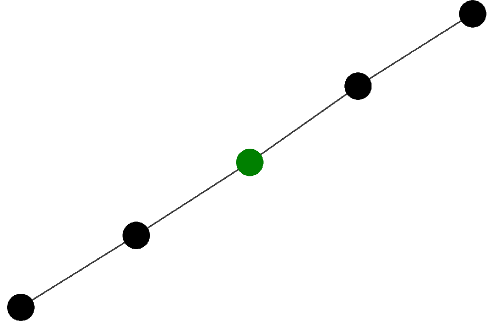
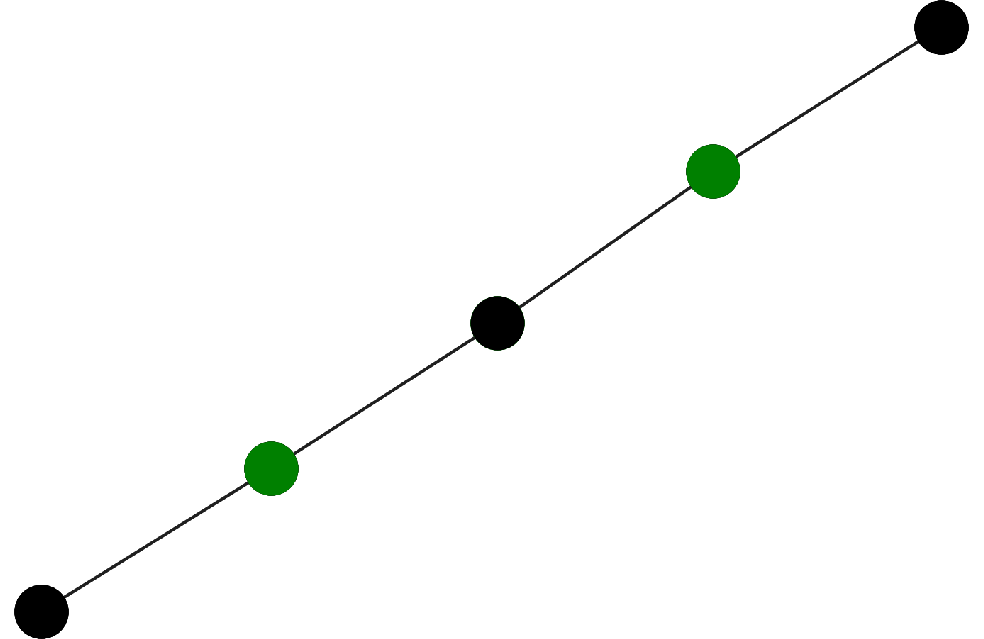
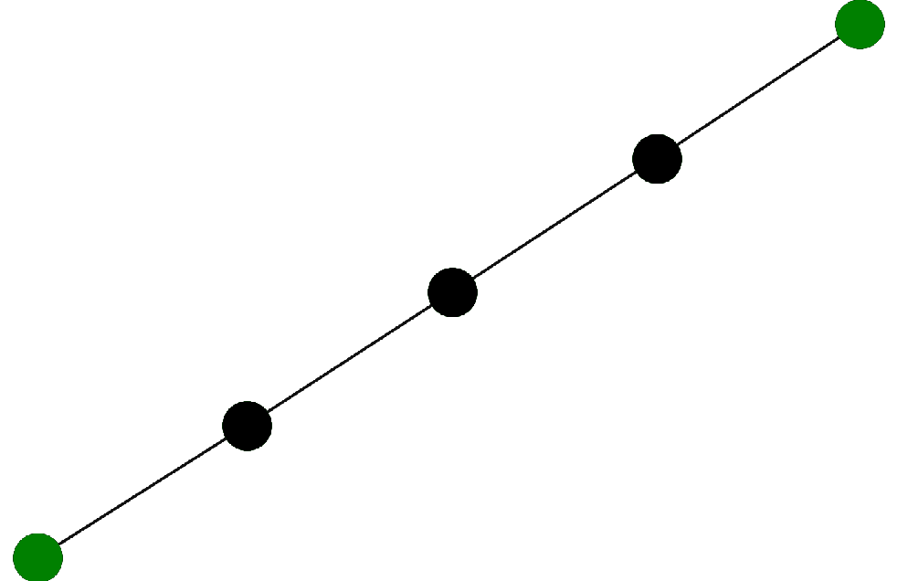
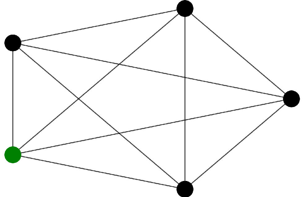
for different graphs and different initial life patterns with single vertex . In Figures 1,2 we color ’alive’ vertices in green and ’dead’ vertices in black.
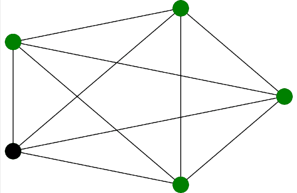
In Figure 1 we illustrate the Game of Life on a line graph. In Figure 2 we show that a single initially alive node in the complete graph makes all other nodes alive and dies itself; the resulting life pattern continues to exist forever without changes. More illustrations are available at https://github.com/mkrechetov/GameOfLifeOnGraphs.
2.2 Universality
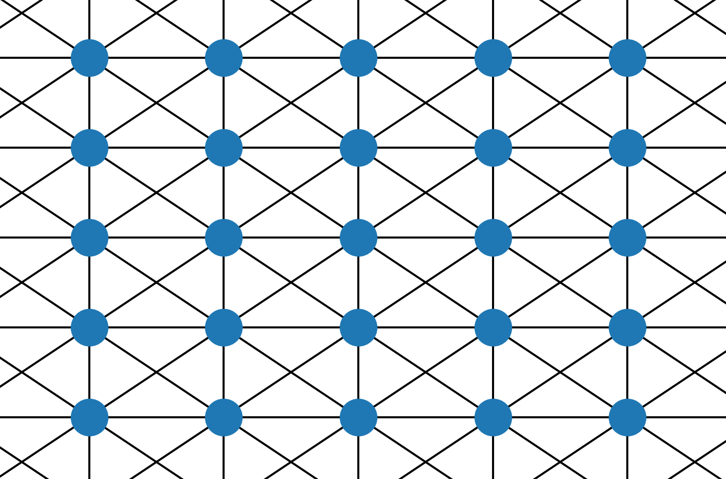
Note that Conway’s Game of Life is an instance of the Game of Life on Graphs. Let us consider an infinite grid graph from the Figure 3, a set of initially alive vertices and an instance . This instance of the Game of Life on Graphs is equivalent to Conway’s Game of Life; now, the proposition below follows:
Proposition. In the most general formulation, the Game of Life on Graphs,
is Turing Complete.
2.3 Halting problem
Definition. Let be an instance of the Game of Life on Graphs. Does the initial population die after some number of iterations or continue to exist forever? We call this question halting of the Game of Life.
Clearly, in the most general formulation (and due to the proposition from the previous section), the halting of the Game of Life is undecidable. However, for finite graphs, the halting problem is in EXPTIME since there is a finite number of possible life patterns; it means that in this case, we can solve halting of the Game of Life simply by simulating the dynamics for (possibly exponential in the size of a graph) number of iterations.
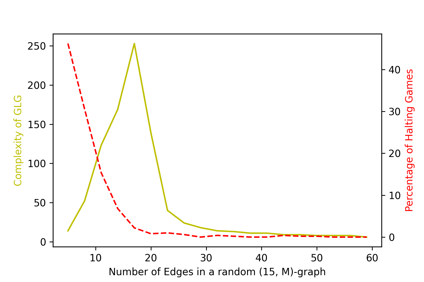
In this section, we study the halting problem for . We select this particular instance in order to be consistent with the following section on Graph Isomorphism testing. We illustrate that the complexity of the Game of Life follows the phase transition behavior with respect to graph density.
Studying phase transitions is a rich topic at the intersection of computer science and statistical physics. Random instances of many different problems and families of structures in computer science undergo a phase transition with respect to one or more parameters. Moreover, the most challenging and complex instances are observed around the transition point, while the instances far from the transition are usually simpler [5, 13, 15].
One of the first famous results on this topic was about 3-SAT phase transition [8, 3]. In that seminal paper, the authors consider random instances of the boolean satisfability problem with variables, clauses, and variables per clause. For large enough values of (what is called thermodynamic limit in physics) the random instances undergo a sharp SAT-UNSAT phase transition with respect to density parameter at some value : for random instances are satisfiable with probability one while for random instances are unsatisfiable with probability one.
Another well-known example is the phase transition in Erdos-Renyi random graphs [11]. Studying the phase transitions of computer science problems is a rich and ongoing line of research; see for example [10] and references therein.
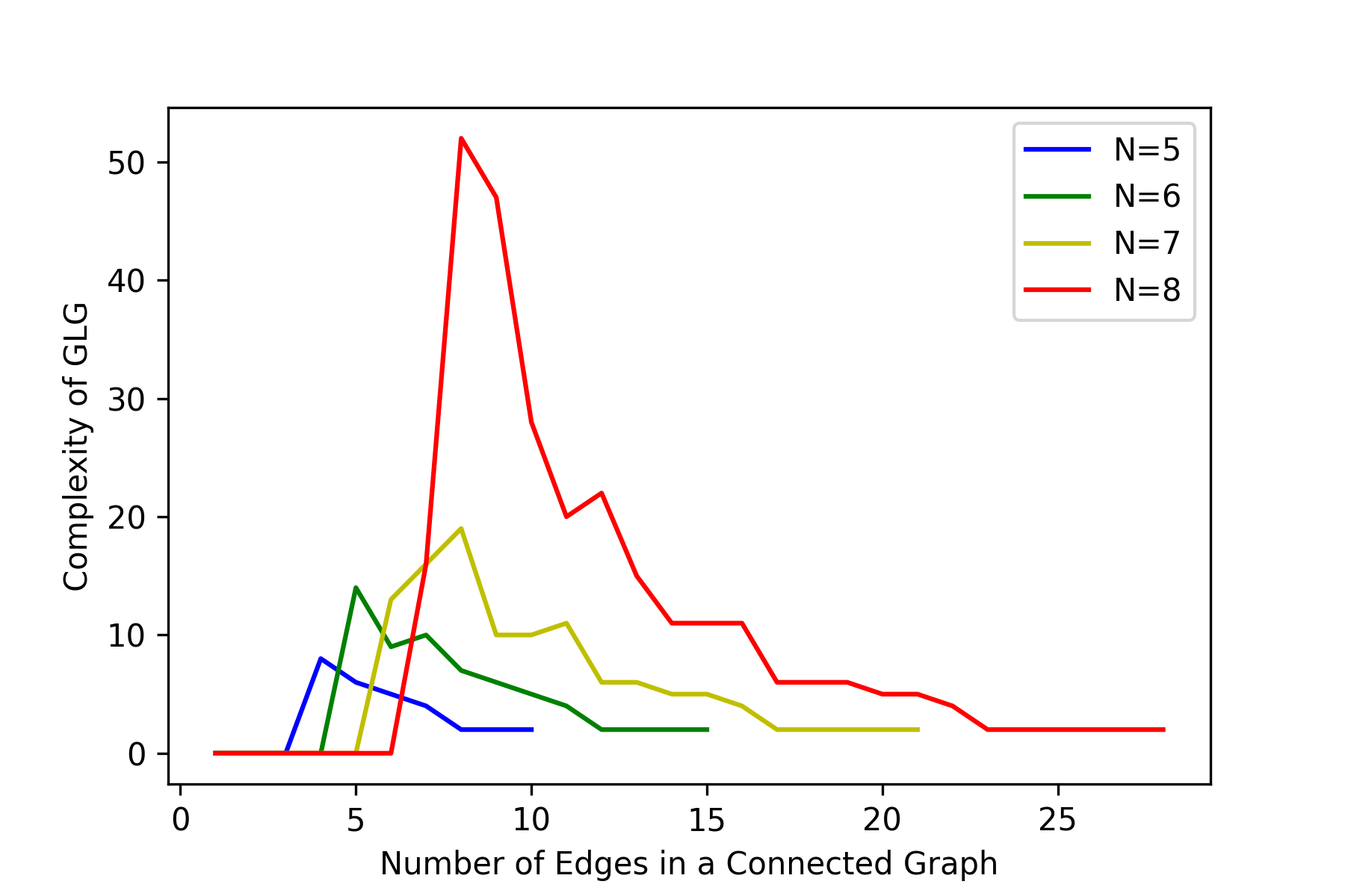
In Figure 4 we illustrate the similar behavior of the Game of Life on Graphs. In the Figure 4(a) we consider the set of all connected graphs with vertices for . For every such graph, we simulate instances of GLG (one for every vertex serving as initially ’alive’). For every GLG we compute its complexity (the number of non-repeating life patterns). We observe that the most complex patterns appear at a particular edge density ().
In the Figure 4(b) we consider random -graphs. For and every we sample 500 random graphs and simulate instances of GLG (one for every vertex serving as initially ’alive’). We compute the number of non-repeating life patterns and the percentage of halting games. We observe the behavior that resembles ensembles of random NP-complete problems and conjecture that the most difficult instances for halting problem appear at the particular density () while for other densities halting can be solved simply simulating the dynamics.
3 Isomorphism Testing
Definition. Two graphs and are called isomorphic iff there exists a bijection , such that for every . Speaking informally, graphs and are isomporhic, if there exists a bijection of vertices that preserves incidence.
The Graph Isomorphism problem is not known to be equivalent to any of NP-complete problems. At the same time, no polynomial algorithm for testing graph isomorphism is known; the best-known algorithm runs in quasipolynomial time [2]. Thus the Graph Isomorphism is known as the problem of intermediate complexity. We refer to [9, 17] as excellent introductions to graph isomorphism and known heuristics.
One of the goals of this paper is to introduce another powerful approach to testing graphs isomorphism. We conjecture that the highly irregular structure of the patterns produced by the Game of Life on Graphs can be used for efficient graph isomorphism testing.
3.1 Feature extraction
There are multiple ways to extract features from the Game of Life on Graphs. In this work, we describe the most straightforward way that is similar to the famous WL algorithm. The approach described in this section is simpler since we consider integer labels instead of multisets and hashes. Meanwhile, our approach generalizes WL algorithms in the following sense: we update labels on vertices with respect to complex life patterns while WL algorithm update depends only on neighbors of a vertex.
Consider a graph , fix the iteration parameter and do the following:
-
1.
Put a real label at every vertex .
-
2.
Fix for every .
-
3.
Initialize instances of the Game of Life on Graphs:
-
4.
Compute steps of evolution for each of instances of .
-
5.
Update labels step by step for iterations and simultaneously for all vertices:
-
6.
(Optionally) Normalize all the the labels at step :
-
7.
For every for a vector . Sort it in the increasing order.
-
8.
The resulting vector of features is the concatencation of vectors for every .
Proposition. If two graphs are isomorphic, all its life patterns coincide under the isomorphism, so are their label sets and the resulting feature vectors.
We describe an isomorphism testing procedure in Algorithm 1. Here we follow our feature extraction algorithm step by step for each of the two graphs. If at a step sorted label sets do not coincide, we have the non-isomorphism certificate. If all the label sets coincide, the graphs are likely to be isomorphic.
False, if graphs and are provably non-isomorphic.
There are various possible generalizations of the feature extraction algorithm above; we list a couple of them:
-
1.
consider multiset labels . Use this sets to get a canonical form or simply calculate co-occurence statistics.
-
2.
Consider as hashes. At step 5) of the feature extraction algorithm, sort hashes and concatenate them.
4 Experiments
We have tested our algorithms on the graph collections from http://users.cecs.anu.edu.au/~bdm/data/graphs.html. We observe that for every pair of non-isomorphic connected graphs with up to ten vertices, Algorithm 1 is able to provide a non-isomorphism certificate in only two steps. The same is true for small connected regular graphs. Our code (python within jupyter notebook) is available at https://github.com/mkrechetov/GameOfLifeOnGraphs.
Another (trivial) observation was that the euclidean distance induced by our feature vectors satisfies triangle inequality for all small connected graphs with up to ten vertices. To measure the distance between two graphs, we compute their feature vectors described in the previous section. Then we calculate the euclidean distance between that two vectors. We call it ’GLG’-distance between two graphs and denote it .
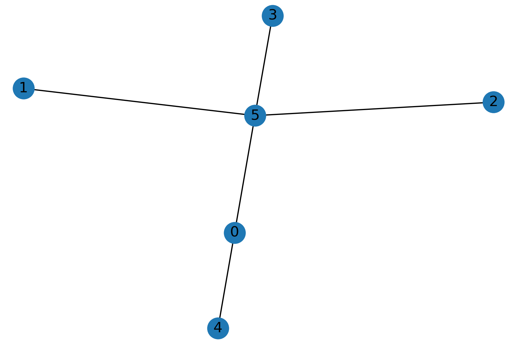
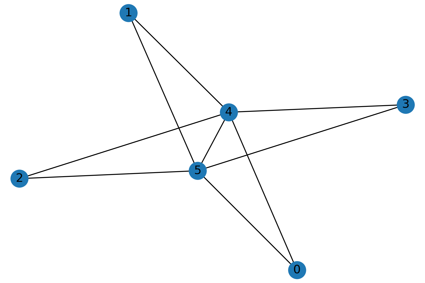
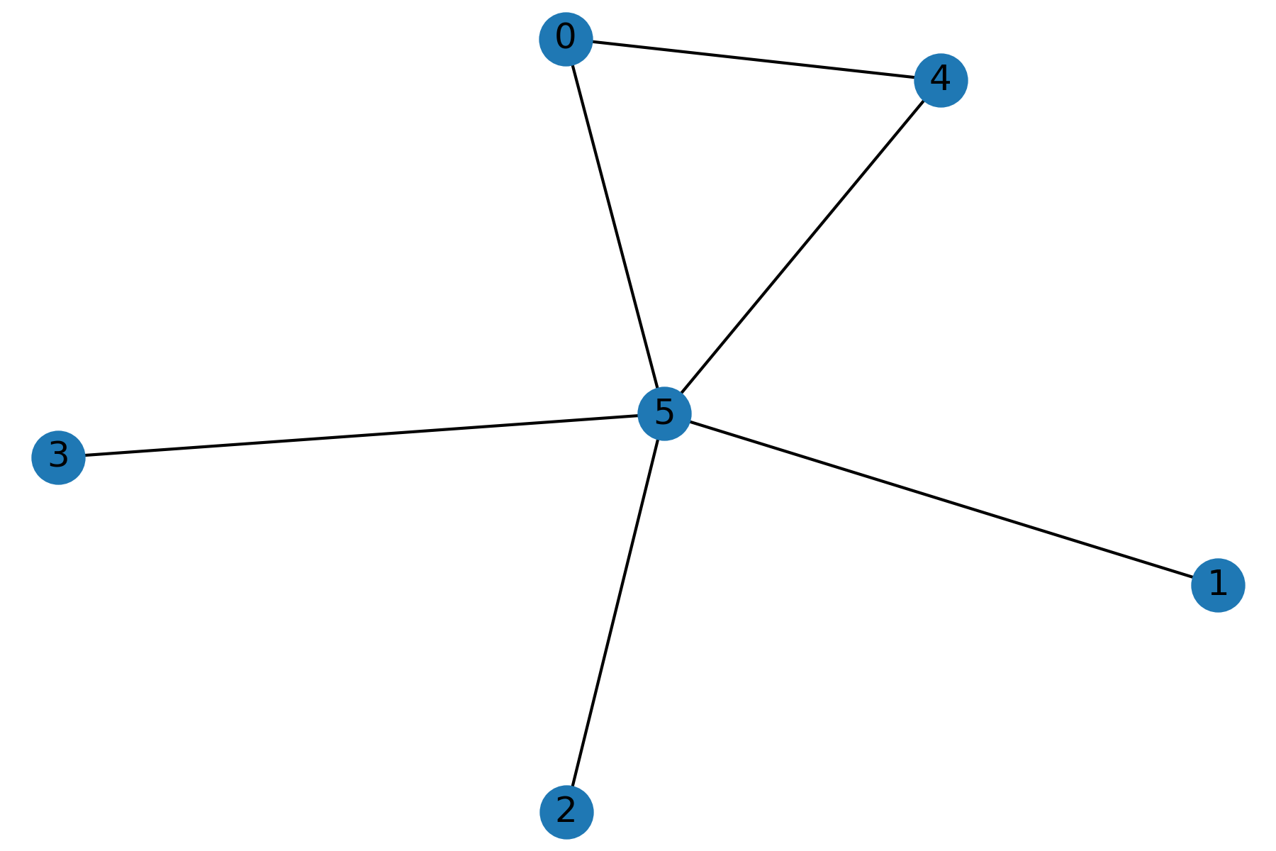
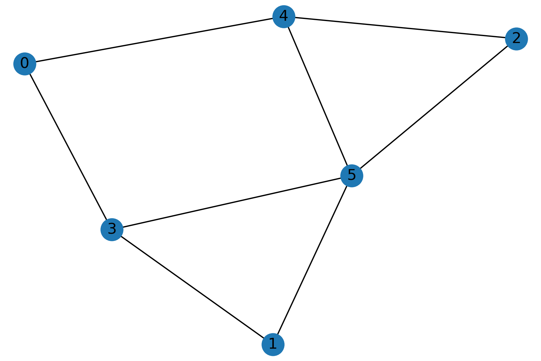
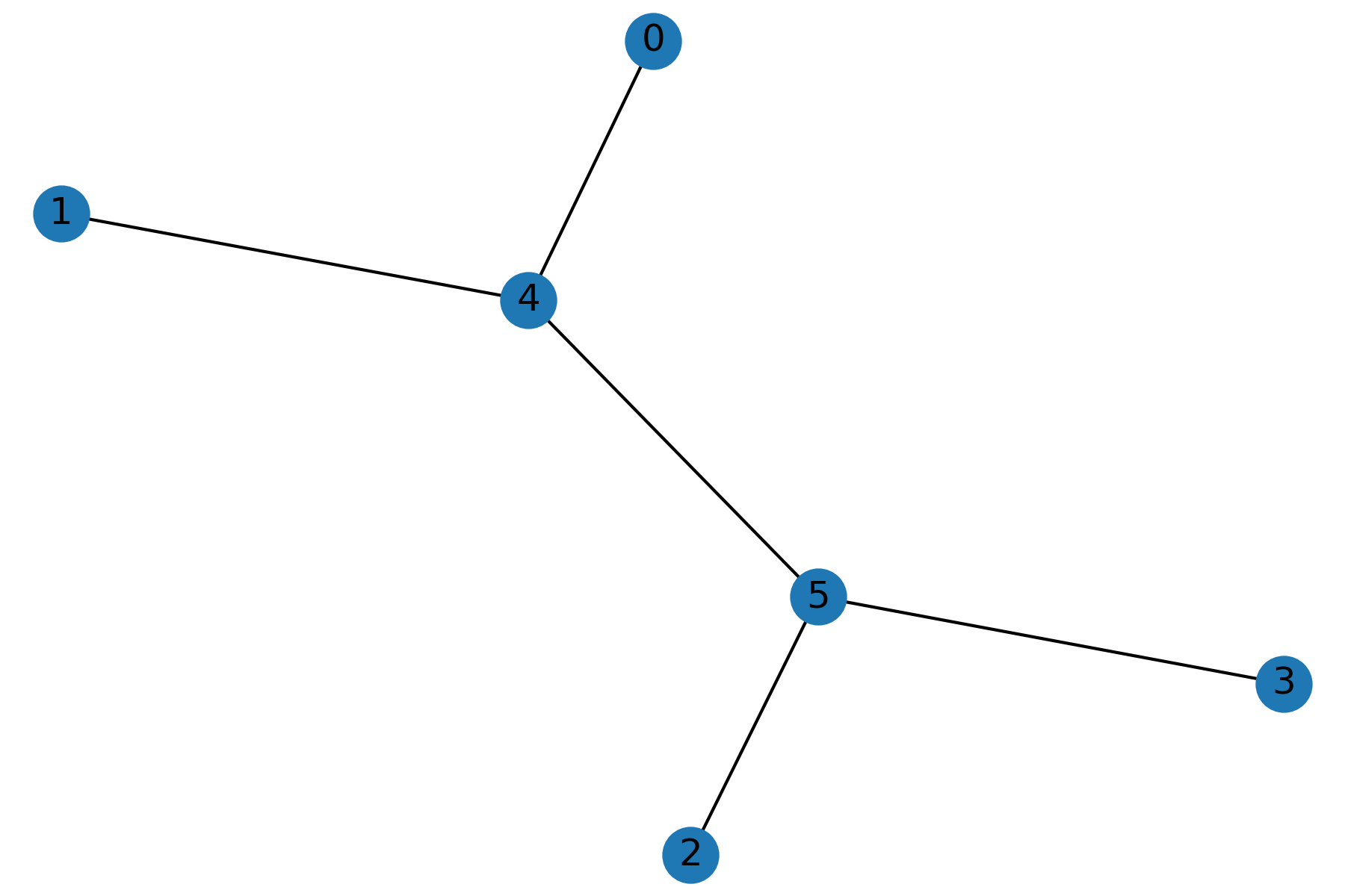
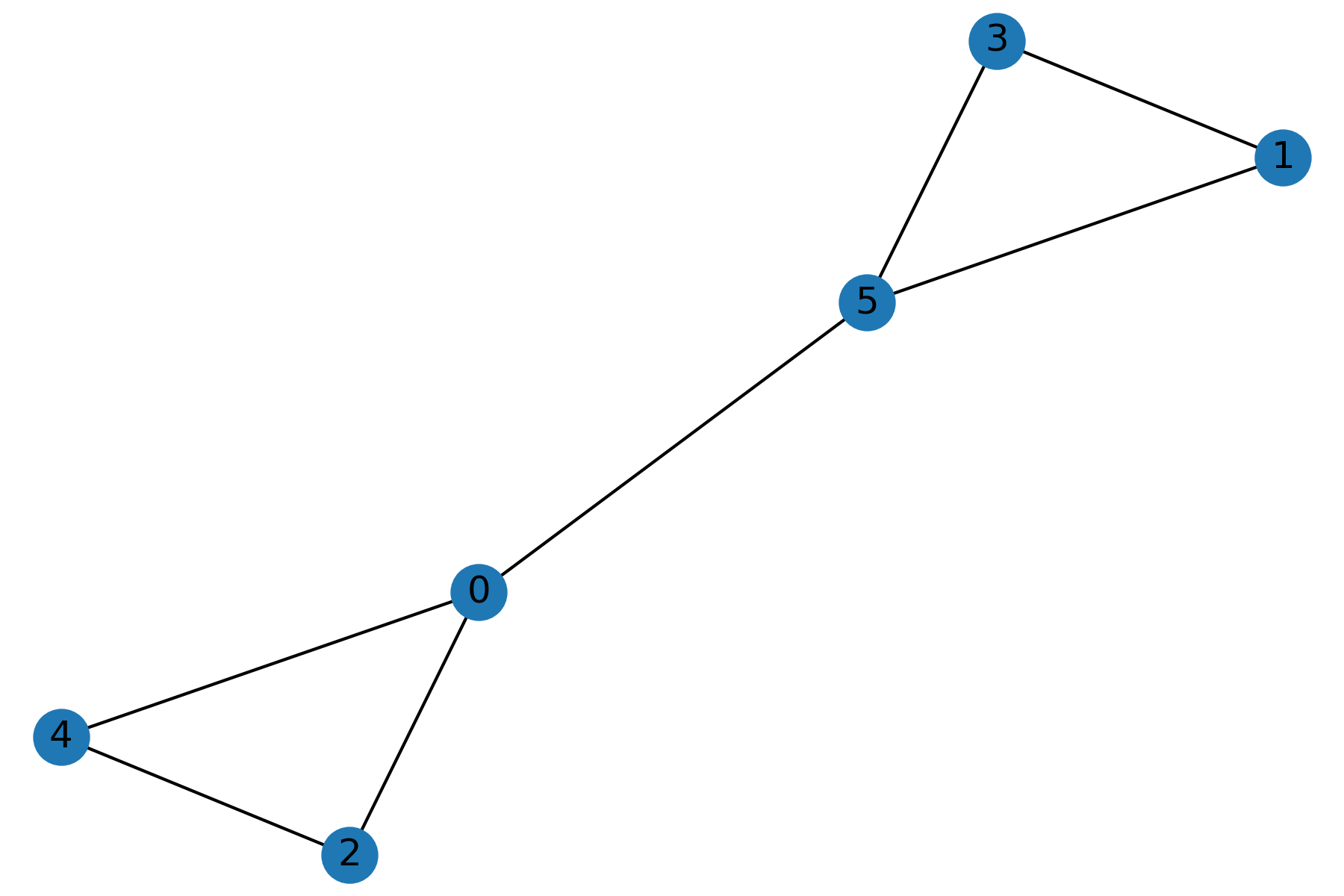
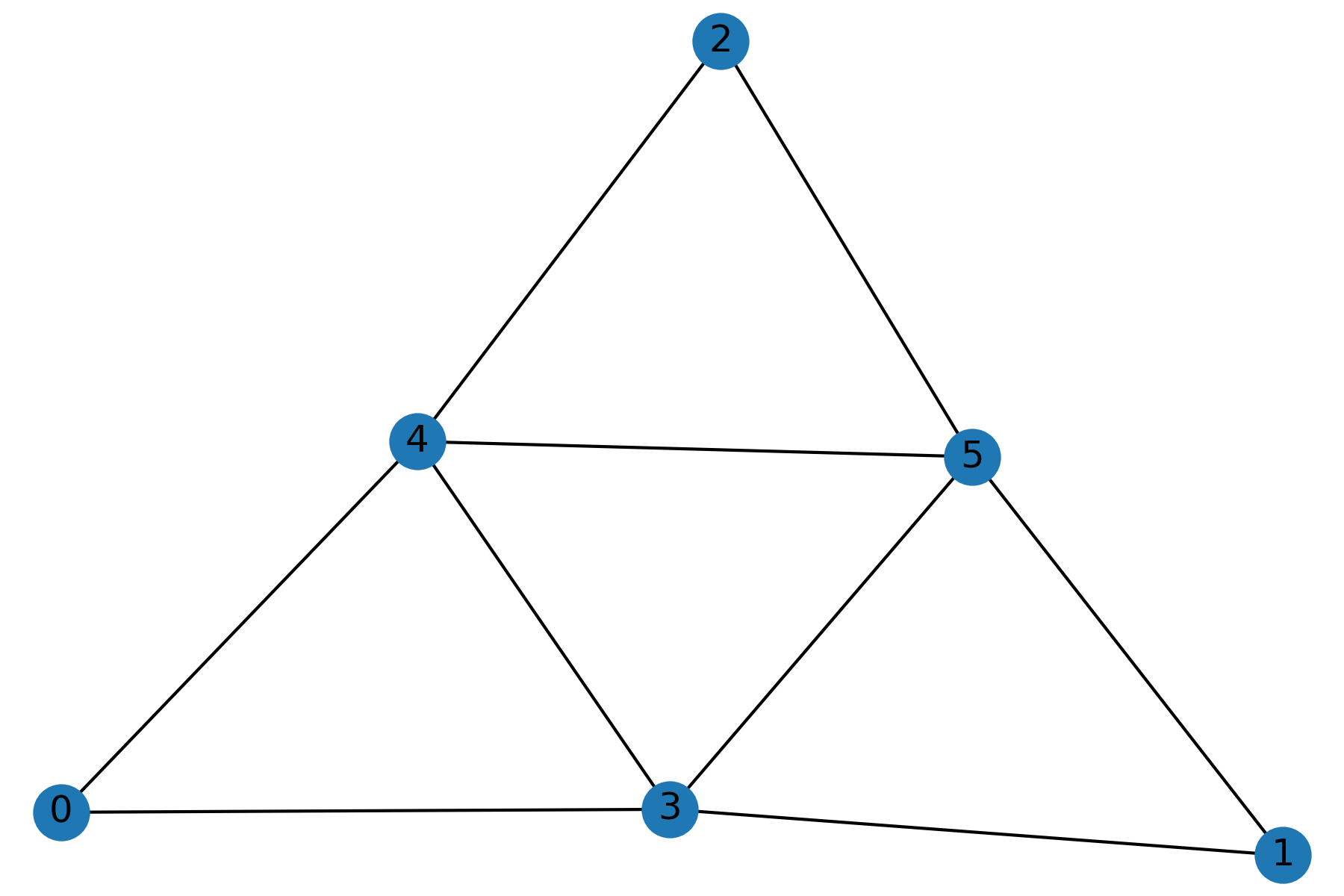
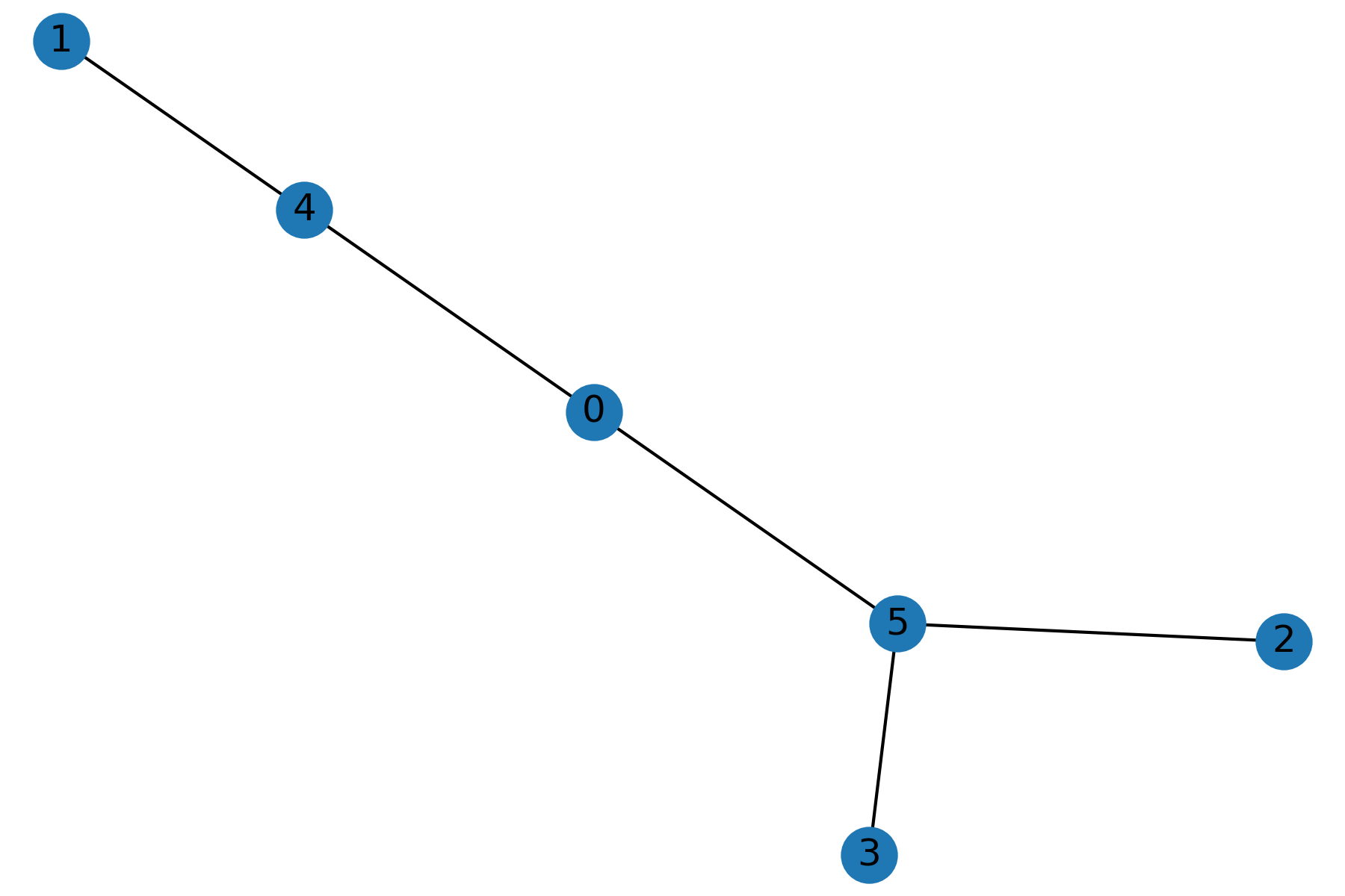
We observe that the triangle inequality becomes equality for some graphs. If a graph triple satisfies the following equality:
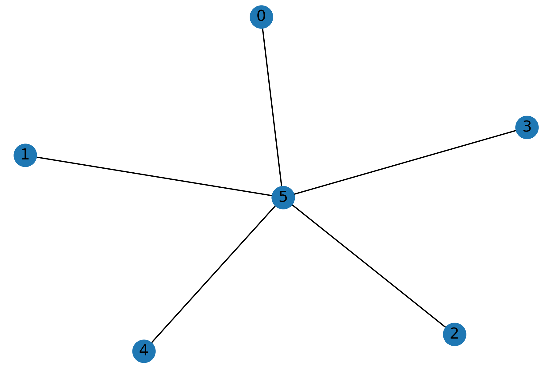
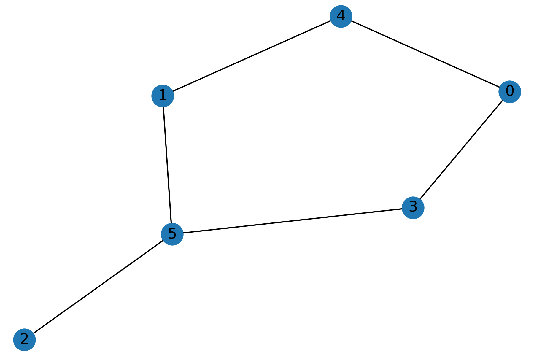
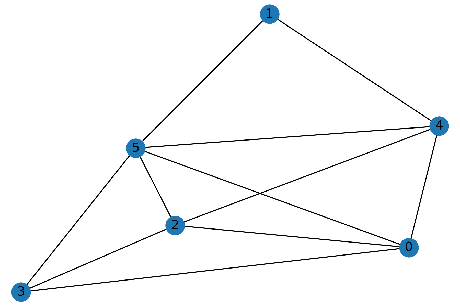
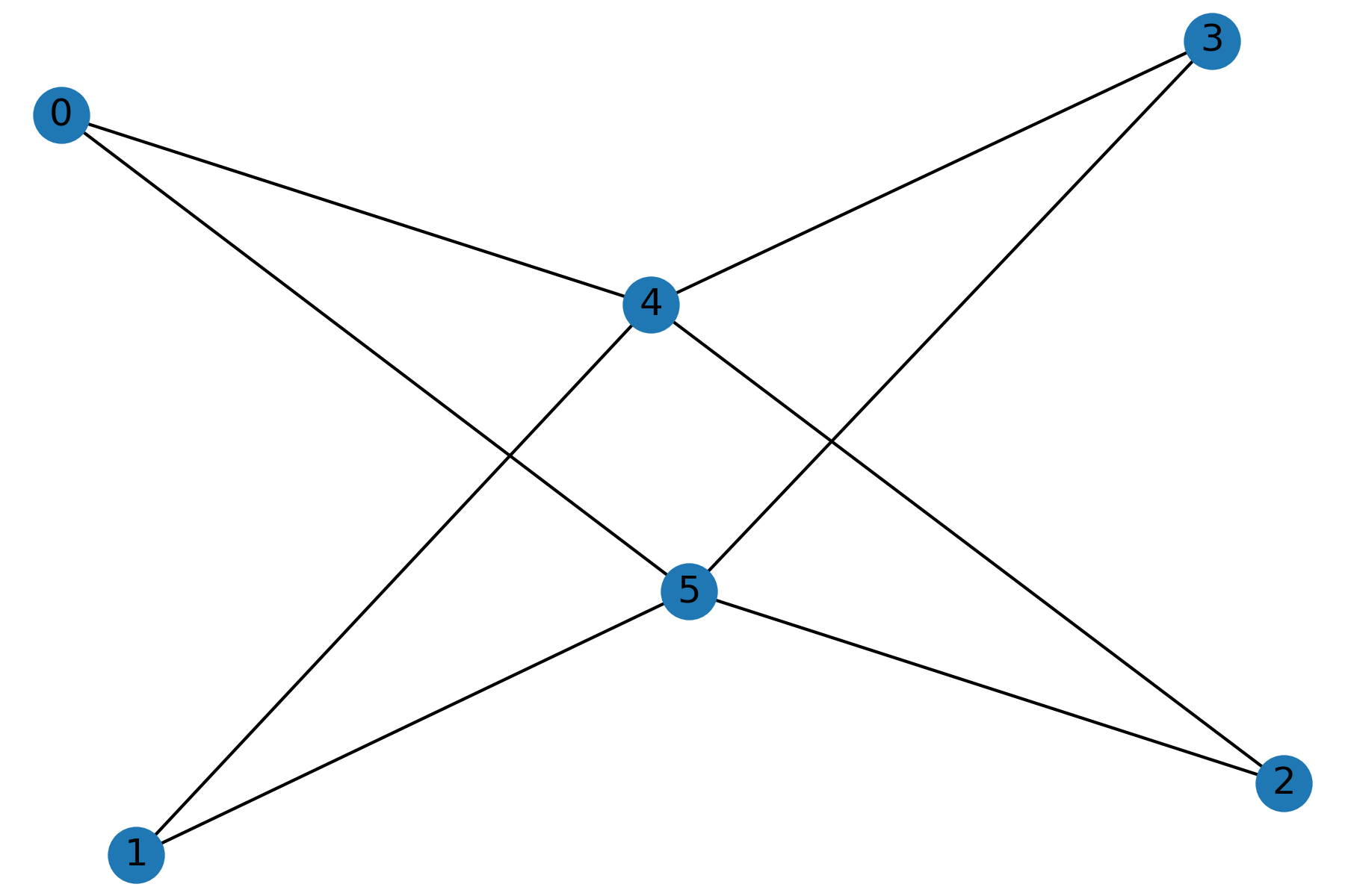
we may interpret the graph as a weighted sum of graphs and . We list some examples in Figure 5 and conjecture that this observation may lead to some future topological interpretations.


5 Conclusions and Path Forward
In this work, we defined the discrete dynamics we call Game of Life on Graphs. We demonstrated how the rich structure of the life patterns could be used for graph isomorphism testing. We also showed that the Game of Life might be used to define metric space on the set of small connected graphs with up to 10 vertices. Hopefully, the concept of the Game of Life on Graphs will find more applications in Graph Theory and Computer Science.
We conclude the manuscript with an incomplete list of further research directions, presented in the order of importance (subjective):
-
•
Are there examples of non-isomorphic graphs that are not distinguished by one or another version of the Game of Life on Graphs? If they exist, then specify the family of graphs for which the Graph Isomorphism problem is solved by the Game of Life on Graphs.
-
•
What is the computational complexity of halting of the Game of Life on Graphs for different values of ? Does the Complexity of GLG undergo the sharp phase transition in the thermodynamic limit ? If so, what is the value of edge density at the transition point?
-
•
Can we use the Game of Life to extract features with good predictive power for graph classification problems? We conjecture that the features extracted from the Game of Life on Graphs are at least as descriptive as the features by DeepWalk [14] and WL kernels [18]. Moreover, the features extracted from the Game of Life are completely deterministic, which can be beneficial for machine learning applications.
-
•
Does the metric induced by the Game of Life on small graphs capture topological properties of graphs? Can the operation of the weighted sum from the Figure 5 be described in a simpler way, e.g., as an operation on edges/cycles of corresponding graphs?
References
- [1] L. Atanassova and K. Atanassov. Intuitionistic fuzzy interpretations of conway’s game of life. International Conference on Numerical Methods and Applications, Springer:232–239, 2010.
- [2] L. Babai. Graph isomorphism in quasipolynomial time. In Proceedings of the forty-eighth annual ACM symposium on Theory of Computing, pages 684–697, 2016.
- [3] J.M. Crawford and L.D. Auton. Experimental results on the crossover point in random 3-sat. Artificial intelligence, 81(1-2)):31–57, 1996.
- [4] B. Durand and Z. Róka. The game of life: universality revisited. Cellular automata, Springer, Dordrecht:51–74, 1999.
- [5] E. Friedgut and J. Bourgain. Sharp thresholds of graph properties, and the k-sat problem. Journal of the American mathematical Society, 12(4):1017–1054, 1999.
- [6] T. Gabor, M.L. Rosenfeld, and C. Linnhoff-Popien. A probabilistic game of life on a quantum annealer. The 2021 Conference on Artificial Life, MIT Press, 2021.
- [7] M. Games. The fantastic combinations of john conway’s new solitaire game “life” by martin gardner. Scientific American, 223:120–123, 1970.
- [8] I.P. Gent and T. Walsh. The sat phase transition. In ECAI, PITMAN, 94:105–109, 1994.
- [9] M. Grohe and P. Schweitzer. The graph isomorphism problem. Communications of the ACM, 63(11):128–134, 2020.
- [10] J.T. Hsieh, S. Mohanty, and J. Xu. Certifying solution geometry in random csps: counts, clusters and balance. arXiv preprint, arXiv:2106.12710, 2021.
- [11] M. Krivelevich and B. Sudakov. The phase transition in random graphs: A simple proof. Random Structures and Algorithms, 43(2):131–138, 2013.
- [12] M. Levene and G. Roussos. A two-player game of life. International Journal of Modern Physics C, 14(02), 2003.
- [13] T. Ohira and R. Sawatari. Phase transition in a computer network traffic model. Physical Review E, 58(1):193, 1998.
- [14] B. Perozzi, R. Al-Rfou, and S. Skiena. Deepwalk: Online learning of social representations. In Proceedings of the 20th ACM SIGKDD international conference on Knowledge discovery and data mining, pages 701–710, 2014.
- [15] H. Philathong, V. Akshay, K. Samburskaya, and J. Biamonte. Computational phase transitions: benchmarking ising machines and quantum optimisers. Journal of Physics: Complexity, 2(1):011002, 2021.
- [16] P. Rendell. Turing universality of the game of life. Collision-based computing, Springer, London:513–539, 2002.
- [17] P. Schweitzer. Problems of unknown complexity: graph isomorphism and ramsey theoretic numbers. PhD thesis, 2009.
- [18] N. Shervashidze, P. Schweitzer, E.J. Van Leeuwen, K. Mehlhorn, and K.M. Borgwardt. Weisfeiler-lehman graph kernels. Journal of Machine Learning Research, 12(9), 2011.
- [19] J.M. Springer and G.T. Kenyon. It’s hard for neural networks to learn the game of life. International Joint Conference on Neural Networks (IJCNN), IEEE:1–8, 2021.