Jinyu Li
Recent Advances in End-to-End Automatic Speech Recognition
Abstract
Recently, the speech community is seeing a significant trend of moving from deep neural network based hybrid modeling to end-to-end (E2E) modeling for automatic speech recognition (ASR). While E2E models achieve the state-of-the-art results in most benchmarks in terms of ASR accuracy, hybrid models are still used in a large proportion of commercial ASR systems at the current time. There are lots of practical factors that affect the production model deployment decision. Traditional hybrid models, being optimized for production for decades, are usually good at these factors. Without providing excellent solutions to all these factors, it is hard for E2E models to be widely commercialized. In this paper, we will overview the recent advances in E2E models, focusing on technologies addressing those challenges from the industry’s perspective.
keywords:
end-to-end, automatic speech recognition, streaming, attention, transducer, transformer, adaptation1 Introduction
The accuracy of automatic speech recognition (ASR) has been significantly boosted since deep neural network (DNN) based hybrid modeling DNN4ASR-hinton2012 was adopted a decade ago. This breakthrough used DNN to replace the traditional Gaussian mixture model for the acoustic likelihood evaluation, while still keeping all the components such as acoustic model, language model, and lexicon model, etc., as the hybrid ASR system. Recently, the speech community has a new breakthrough by transiting from hybrid modeling to end-to-end (E2E) modeling graves2014towards ; hannun2014deep ; chorowski2014end ; miao2015eesen ; bahdanau2016end ; chan2016listen ; collobert2016wav2letter ; prabhavalkar2017comparison which directly translates an input speech sequence into an output token sequence using a single network. Such a breakthrough is even more revolutionary because it overthrows all the modeling components in traditional ASR systems, which have been used for decades.
There are several major advantages of E2E models over traditional hybrid models. First, E2E models use a single objective function which is consistent with the ASR objective to optimize the whole network, while traditional hybrid models optimize individual components separately, which cannot guarantee the global optimum. Therefore, E2E models have been shown to outperform traditional hybrid models not only in academics watanabe2017hybrid but also in the industry sainath2020streaming ; Li2020Developing . Second, because E2E models directly output characters or even words, it greatly simplifies the ASR pipeline. In contrast, the design of traditional hybrid models is complicated, requiring lots of expert knowledge with years of ASR experience. Third, because a single network is used for ASR, E2E models are much more compact than traditional hybrid models. Therefore, E2E models can be deployed to devices with high accuracy.
While E2E models achieve the state-of-the-art results in most benchmarks in terms of ASR accuracy, hybrid models are still used in a large proportion of commercial ASR systems at the time of writing because the ASR accuracy is not the only factor for the production choice between hybrid and E2E models. There are lots of practical factors such as streaming, latency, adaptation capability, etc., which affect the commercial model deployment decision. Traditional hybrid models, optimized for production for decades, are usually good at these factors. Without providing excellent solutions to all these factors, it is hard for E2E models to be widely commercialized. To that end, in this paper, we overview popular E2E models with a focus on the technologies addressing those challenges from the perspective of the industry.
2 End-to-end models
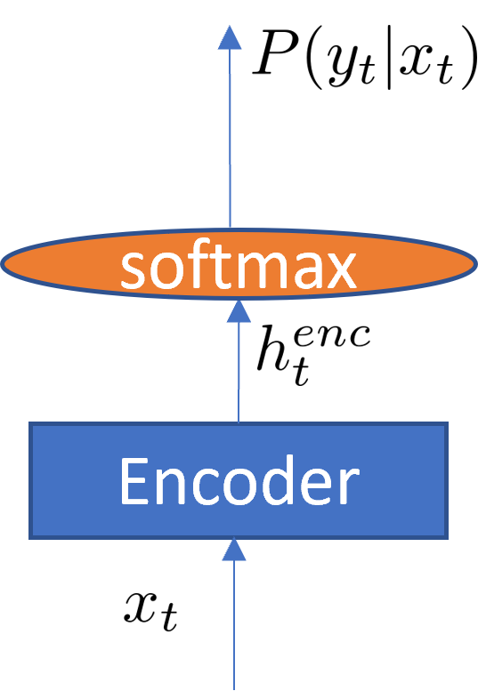
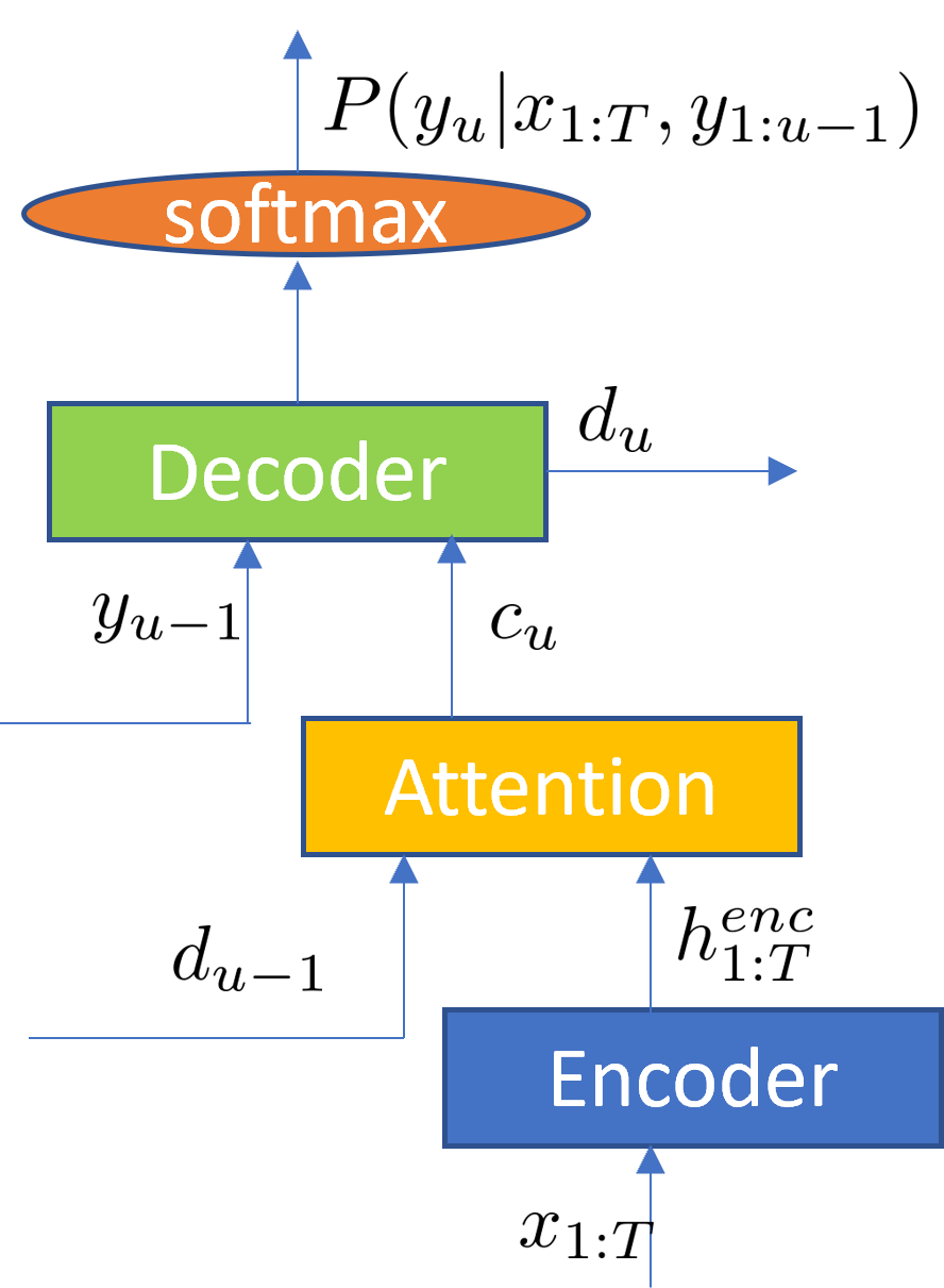
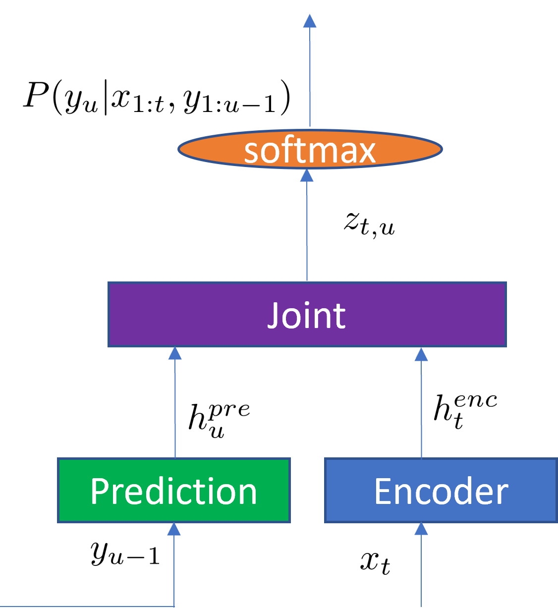
The most popular E2E techniques for ASR are: (a) Connectionist Temporal Classification (CTC) graves2006connectionist , (b) Attention-based Encoder-Decoder (AED) cho2014learning ; Attention-bahdanau2014 , and (c) recurrent neural network Transducer (RNN-T) Graves-RNNSeqTransduction . Among them, RNN-T provides a natural solution to streaming ASR with high accuracy and low latency, ideal for industrial application. These three most popular E2E techniques are illustrated in Figure 1. In this section, we will give a short overview of them.
2.1 Connectionist Temporal Classification
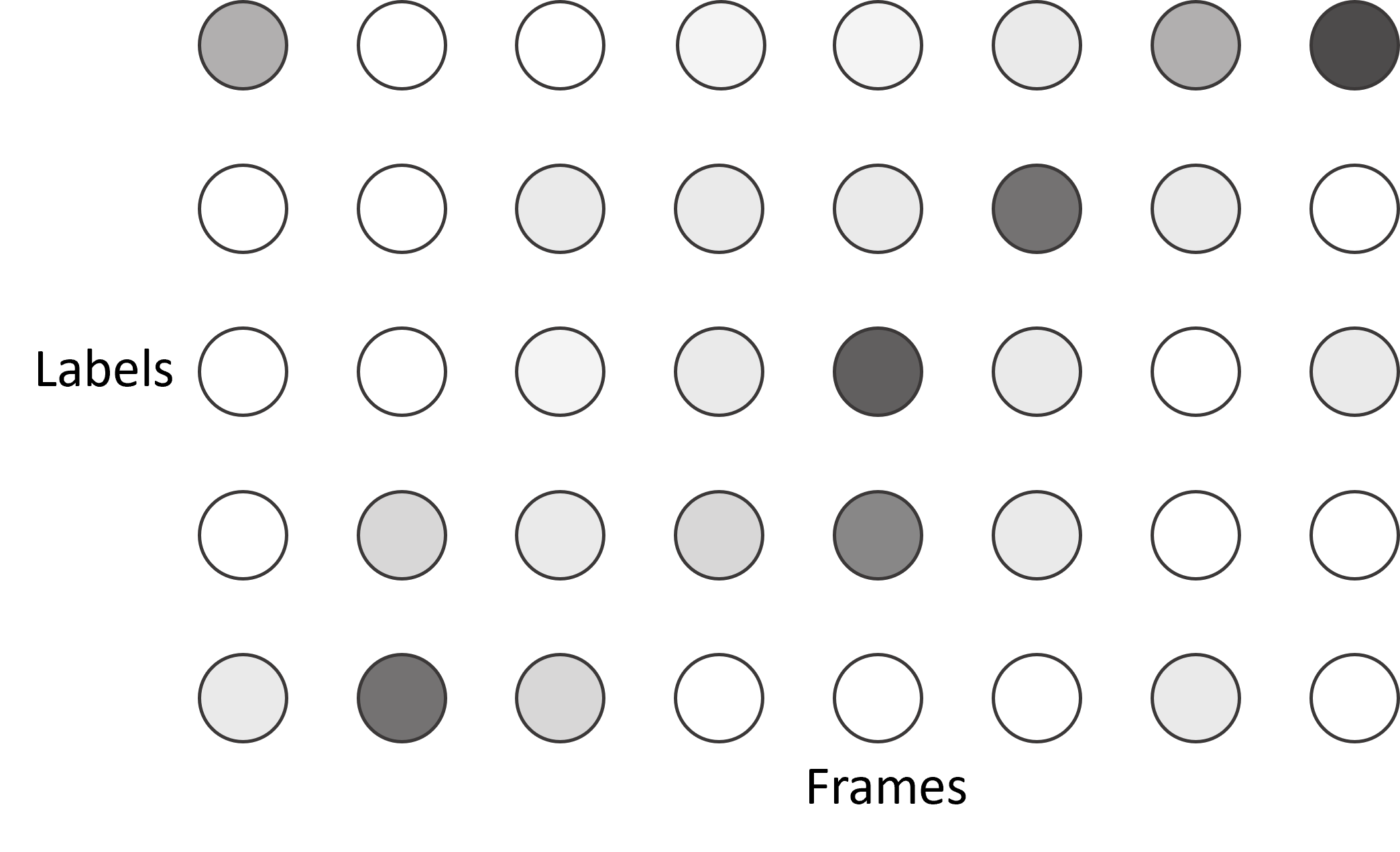
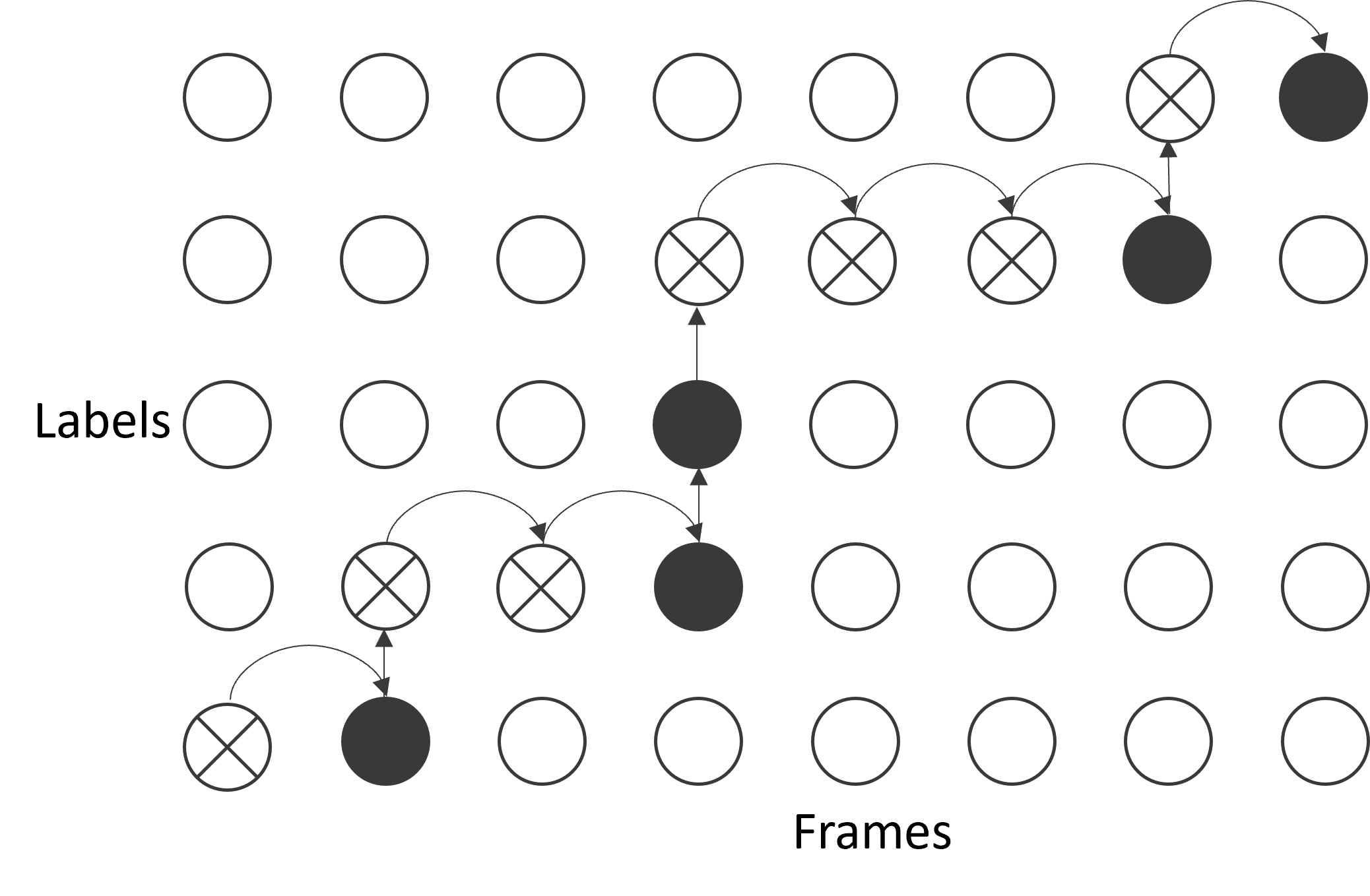
The Connectionist Temporal Classification (CTC) technique for ASR graves2014towards was designed to map the speech input sequence into an output label sequence. Because the length of output labels is smaller than that of the input speech sequence, a blank label is inserted between output labels with allowable repetition of labels to construct CTC paths that have the same length as the input speech sequence. Figure 2 shows an example of three CTC paths for the word “team”.
Figure 1(a) shows the architecture of CTC. We denote the input speech sequence as , the original output label sequence as , and all of the CTC paths mapped from as . The encoder network is used to convert the acoustic feature into a high-level representation . The CTC loss function is defined as the negative log probabilities of correct labels given the input speech sequence:
| (1) |
with
| (2) |
where is a CTC path. With the conditional independence assumption, can be decomposed into a product of frame posterior as
| (3) |
where is the length of the speech sequence.
CTC is the first E2E technology widely used in ASR hannun2014deep ; miao2015eesen ; soltau2016neural ; zweig2017advances ; zeyer2017ctc ; li2018advancing ; audhkhasi2018building . However, the conditional independence assumption in CTC is most criticized. One way to relax that assumption is to use the attention mechanism Das18advancing ; salazar2019self which can introduce implicit language modeling across speech frames. Such attention-based CTC models implicitly relax the conditional independence assumption by improving the encoder without changing the CTC objective function, and therefore enjoy the simplicity of CTC modeling. By replacing the underlying long short-term memory (LSTM) Hochreiter1997long with Transformer vaswani2017attention in the encoder, which allows a more powerful attention mechanism to be used, CTC thrives again in recent studies higuchi2020mask . It gets further boosted by the emerged self-supervised learning technologies baevski2020wav2vec ; chung2020generative ; zhang2020pushing ; hsu2021hubert which can learn a very good representation that carries semantic information.
2.2 Attention-based Encoder-Decoder
The attention-based encoder-decoder (AED) model is another type of E2E ASR model chorowski2014end ; bahdanau2016end ; chan2016listen ; lu2016training ; zeyer2018improved . As shown in Figure 1(b), AED has an encoder network, an attention module, and a decoder network. The AED model calculates the probability as
| (4) |
where is the output label index. The training objective is also to minimize .
The encoder network performs the same function as the encoder network in CTC by converting input feature sequences into high-level hidden feature sequences. The attention module computes attention weights between the previous decoder output and the encoder output of each frame using attention functions such as additive attention bahdanau2016end or dot-product attention chan2016listen , and then generates a context vector as a weighted sum of the encoder outputs. The decoder network takes the previous output label together with the context vector to generate its output to calculate , which is operated in an autoregressive way as a function of the previous label outputs without the conditional independence assumption.
While the attention on the full sequence in AED is a natural solution to machine translation which has the word order switching between source and target languages, it may not be ideal to ASR because the speech signal and output label sequence are monotonic. In order to have better alignment between the speech signal and label sequence, the AED model is optimized together with a CTC model in a multi-task learning framework by sharing the encoder kim2017joint . Such a training strategy greatly improves the convergence of the attention-based model and mitigates the alignment issue. It becomes the standard training recipe for most AED models watanabe2017hybrid ; hori2017advances ; toshniwal2017multitask ; ueno2018acoustic ; delcroix2018auxiliary ; liu2019adversarial ; kim2019attention ; karita2019improving . In hori2017joint , a further improvement was proposed by combining the scores from both the AED model and the CTC model during decoding.
Most commercial setups need ASR systems to be streaming with low latency, which means ASR systems should produce the recognition results at the same time as the user is speaking. In vanilla AED models, the attention is applied to the whole utterance in order to achieve good performance. The latency can be significant because such a setup needs to obtain the full utterance before decoding, and it is impractical for streaming ASR scenarios where the speech signal comes in a continuous mode without segmentation. There are lots of attempts to build streaming AED models. The basic idea of these methods is applying attention on the chunks of the input speech. The difference between these attempts is the way the chunks are determined and used for attention. Figure 3(a) shows the full attention of AED, which spreads attention weights across the whole utterance. One major school of streaming AED models is to use monotonic attention. In raffel2017online , a monotonic attention mechanism was proposed to use integrated decision for triggering ASR. Attention is only on the time step corresponding to the trigger point as shown in Figure 3(b). The method was improved in chiu2018monotonic , where a monotonic chunkwise attention (MoChA) method was proposed to stream the attention by splitting the encoder outputs into small fixed-size chunks so that the soft attention is only applied to those small chunks, as shown in Figure 3(c). Adaptive-size instead of fixed-size chunks were used in fan2019online . Recently, monotonic infinite lookback (MILK) attention arivazhagan2019monotonic was proposed to attend the entire sequence preceding the trigger point, as shown in Figure 3(d). Another popular streaming AED method is triggered attention moritz2019triggered which uses CTC segments to decide the chunks and is applied to lots of AED models moritz2019streaming ; moritz2020streaming ; hori2021advanced .
While all these methods can achieve the goal of streaming ASR to some extent, they usually do not enforce low-latency which is another important factor for commercial ASR systems. This challenge was addressed in inaguma2020minimum , which proposed to train low-latency streaming AED models by leveraging the external hard alignment. In wang2020low , a scout network was used to predict word boundary which is then used by the ASR network to predict the next subword by utilizing the information from all speech frames before it for low latency streaming.
All streaming AED models need some complicated strategies to decide the trigger point for streaming. A comparison of streaming ASR methods was conducted in kim2021comparison which shows RNN Transducer has advantages over MoChA in terms of latency, inference time, and training stability. AED models also cannot perform well on long utterances chiu2019comparison ; narayanan2019recognizing . Therefore, although there are still many activities li2019end ; kim2019attention ; dong2020cif ; miao2020transformer ; tian2020synchronous ; moritz2020streaming ; inaguma2020enhancing ; li2021transformer ; tsunoo2021streaming ; sterpu2021learning ; kashiwagi2021gaussian in the area of streaming AED models, the industry tends to choose RNN Transducer introduced next as the dominating streaming E2E model while AED has its position in some non-streaming scenarios.
2.3 RNN Transducer
RNN Transducer (RNN-T) Graves-RNNSeqTransduction provides a natural way for streaming ASR because its output conditions on the previous output tokens and the speech sequence until the current time step (i.e., frame) as . In this way, it also removes the conditional independence assumption of CTC. With the natural streaming capability, RNN-T becomes the most popular E2E model in the industry prabhavalkar2017comparison ; battenberg2017exploring ; he2019streaming ; Li2019improving ; sainath2020streaming ; Li2020Developing ; zhang2021benchmarking ; saon2021advancing ; punjabi2021joint .
Illustrated in Figure 1(c), RNN-T contains an encoder network, a prediction network, and a joint network. The encoder network is the same as that in CTC and AED, generating a high-level feature representation . The prediction network produces a high-level representation based on RNN-T’s previous output label . The joint network is a feed-forward network that combines and as
| (5) |
where and are weight matrices, is a bias vector, and is a non-linear function (e.g., RELU or Tanh). is connected to the output layer with a linear transform
| (6) |
where and denote a weight matrix and a bias vector, respectively. The probability of each output token is
| (7) |
The loss function of RNN-T is also , with
| (8) |
as the sum of all possible alignment paths that are mapped to the label sequence . The mapping from the alignment path to the label sequence is defined as . 111Note this mapping is different from the CTC mapping in Eq. (2).
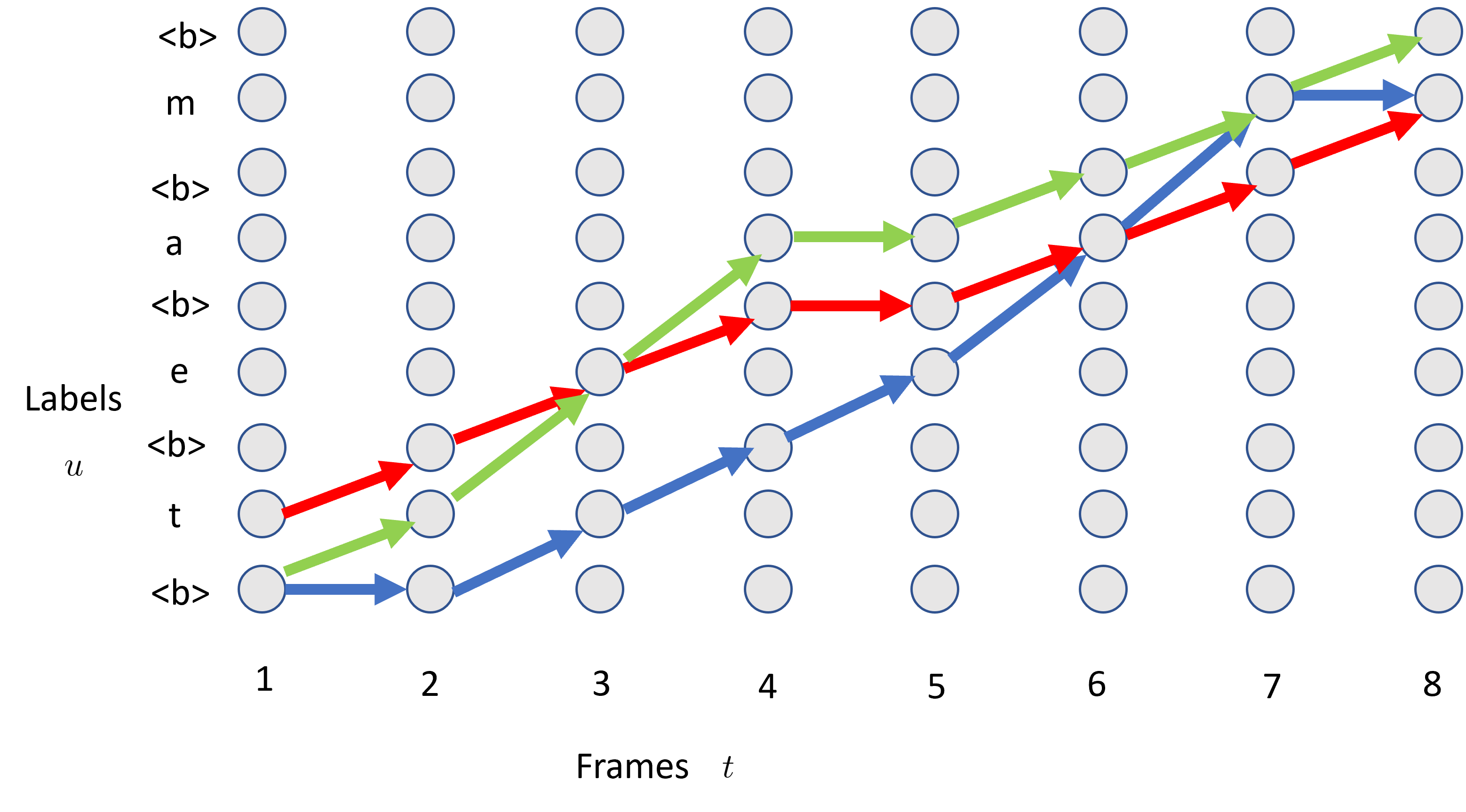
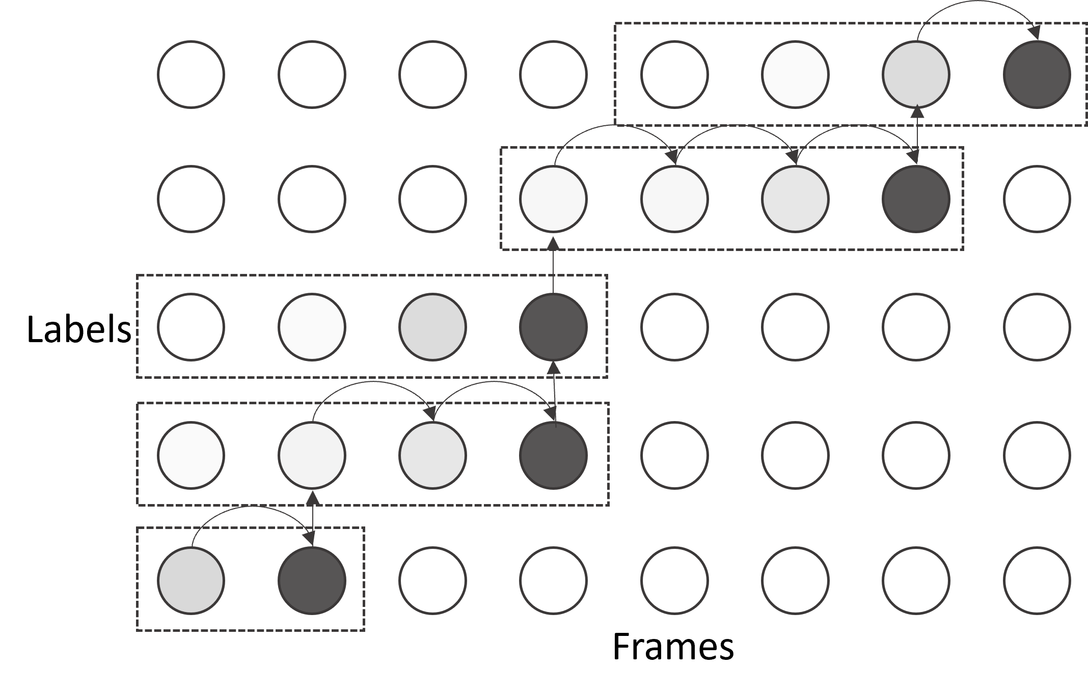
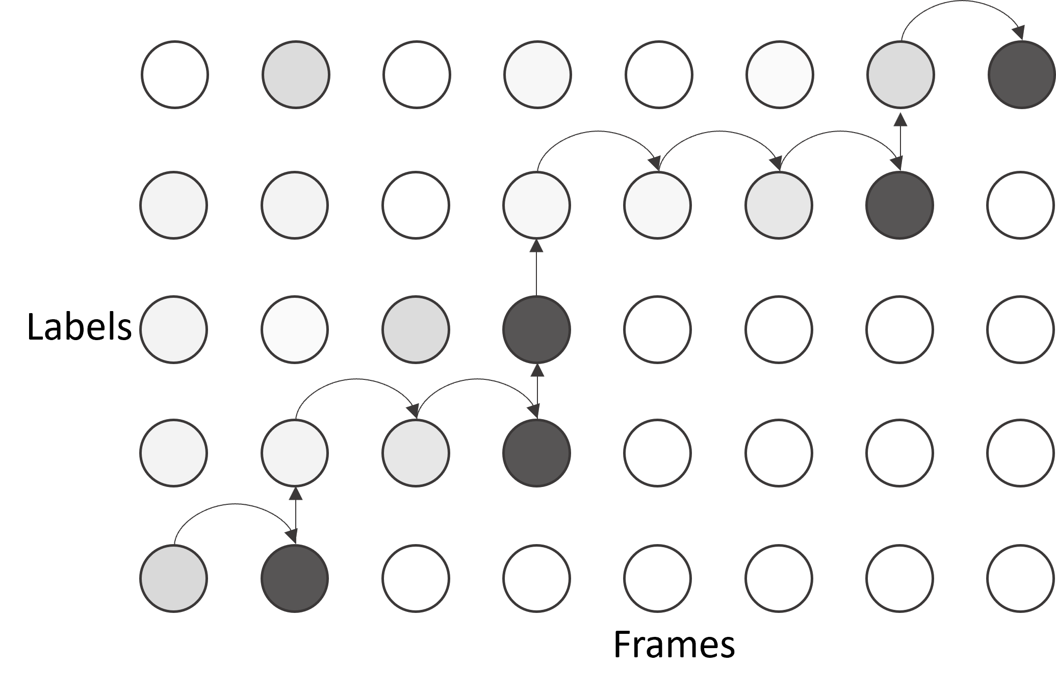
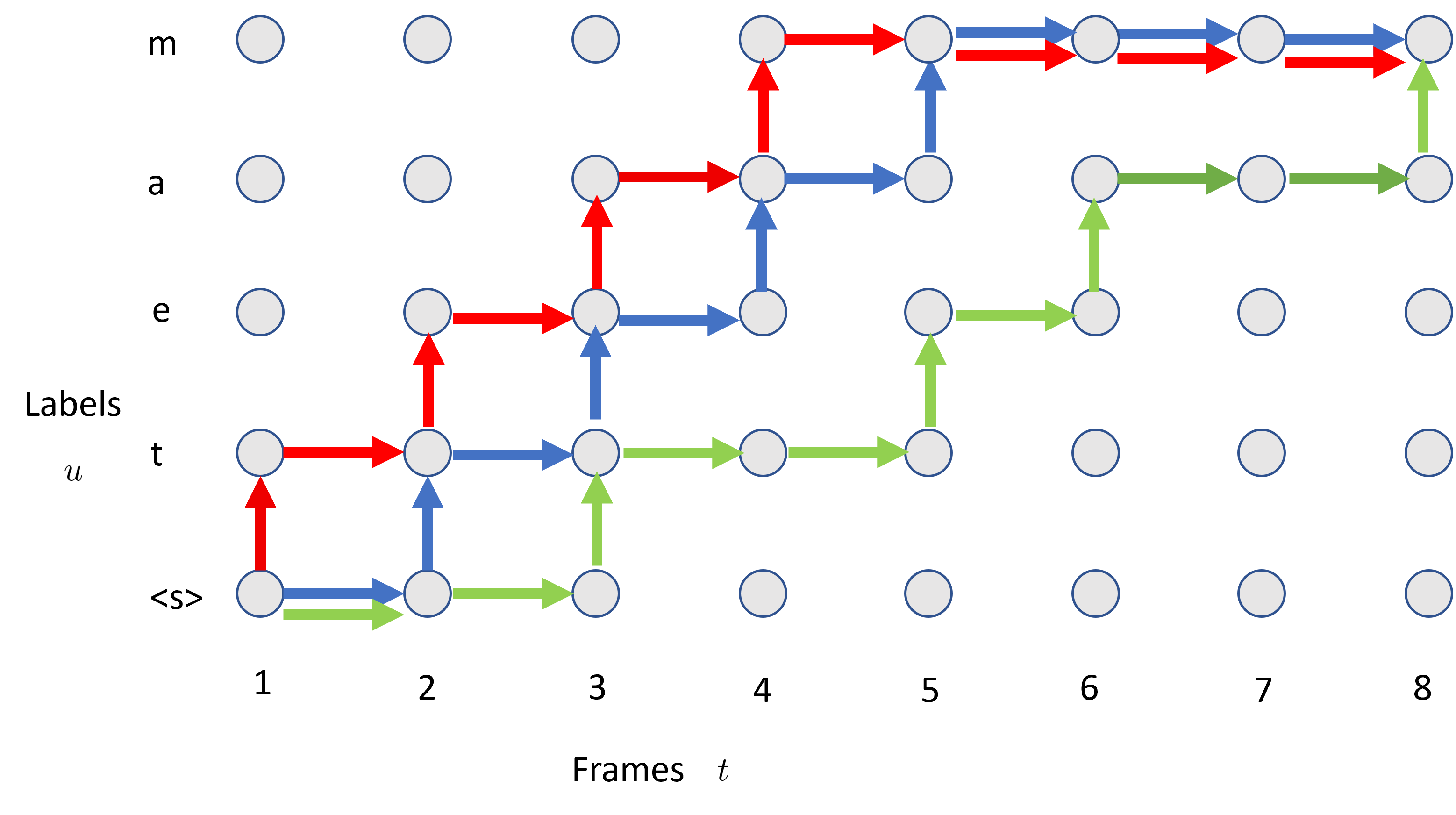
In Figure 4, three example alignment paths are plotted for speech sequence and label sequence , where is a token for sentence start. All valid alignment paths go from the bottom left corner to the top right corner of the grid, hence the length of each alignment path is . In an alignment path, the horizontal arrow advances one time step with a blank label by retaining the prediction network state while the vertical arrow emits a non-blank output label.
The posteriors of the alignment grid composed by the encoder and prediction networks need to be calculated at each grid point. This a three-dimensional tensor that requires much more memory than what is needed in the training of other E2E models such as CTC and AED. Eq. (8) is calculated based on the forward-backward algorithm described in Graves-RNNSeqTransduction . In bagby2018efficient , to improve training efficiency, the forward and backward probabilities can be vectorized with a loop skewing transformation, and the recursions can be computed in a single loop instead of two nested loops. Function merging was proposed in Li2019improving to significantly reduce the training memory cost so that larger minibatches can be used to improve the training efficiency.
It is worth noting that ASR latency is a very important metric that affects user experience. If the latency is large, users will feel the ASR system is not responding. Therefore, practical systems need to have a small latency in order to give users a good experience sainath2021efficient . Shangguan et al. recently gave a very good study of the factors affecting user perceived latency in shangguan2021dissecting . In chang2019joint , RNN-T is designed to generate end of sentence (EOS) token together with the ASR transcription. The latency of EOS detection is improved in li2020towards with early and late penalties. While RNN-T is now the most natural E2E model for streaming, the vanilla RNN-T still has latency challenges because RNN-T tends to delay its label prediction until it is very confident by visiting more future frames of the current label. The green path in Figure 4 is an example alignment of such a delayed decision. In order to ensure low latency for RNN-T, constrained alignment sainath2020emitting ; mahadeokar2021alignment was proposed to restrict the training alignment within a delay threshold of the ground truth time alignment and forbid other alignment paths. Strict alignment between the input speech sequence and output label sequence is enforced in tripathi2019monotonic to generate better alignment for streaming RNN-T. In addition to the benefit of latency, another advantage of all these alignment restricted RNN-T methods is GPU-memory saving and training speed-up because less alignment paths are used during training. FastEmit yu2021fastemit was proposed to reduce latency without the need of the ground truth alignment. It encourages the emission of vocabulary tokens and discourages the blank transition at all positions in the time-label grid. Therefore, it pushes all alignment paths to the left direction of the time-label grid. However, this operation is a little aggressive at reducing latency, which can result in recognition accuracy loss. In kim2021reducing , a self-alignment method was proposed to reduce latency in a mild way. It uses the self alignment of the current model to find the lower latency alignment direction. In Figure 4, the blue path indicates a self-alignment path and the red path is one frame left to the self-alignment path. During training, the method encourages the left-alignment path, pushing the model’s alignment to the left direction. The proposed method was reported to have better accuracy and latency tradeoff than the constrained-alignment method and FastEmit.
In addition to these three popular E2E models, there are also other E2E models such as neural segmental model tang2017end and recurrent neural aligner sak2017recurrent , to name a few.
3 Encoder
In all E2E ASR models, the most important component is the encoder which converts speech input sequences into high-level feature representations.
3.1 LSTM
In early E2E ASR works, LSTM is the most popular model unit. The encoder can be either a multi-layer unidirectional LSTM-RNN as Eq. (9)
| (9) |
or a multi-layer bidirectional LSTM (BLSTM)-RNN as Eq. (10)
| (10) |
where denotes the standard LSTM unit with an optional projection layer Sak2014long . Here, is the hidden output of the -th () layer at time and is the input vector for the -th layer with
| (11) |
where is the speech input at time step . The last layer output, , is used as the encoder output.
Because of the streaming request in most commercial ASR systems, unidirectional LSTM is used more widely. When the encoder is an LSTM-RNN, CTC and RNN-T work in the streaming mode by default while AED still needs streaming attention strategies in order to work in the streaming mode. In contrast, when the encoder is a BLSTM-RNN, all E2E models are non-streaming models.
There is a clear accuracy gap between the LSTM encoder and the BLSTM encoder because the latter uses the whole utterance information to generate the encoder output. In order to reduce the gap, it is a natural idea to use future context frames to generate more informative encoder output with the methods such as latency controlled BLSTM (LC-BLSTM) zhang2016highway or contextual LSTM (cLSTM) li2019improvinglayer ; Li2020Developing . LC-BLSTM works in an overlapped multi-frame chunk mode. BLSTM is still used within a chunk, while the state of the forward direction is carried across chunks. In contrast, cLSTM works in a frame-by-frame uni-directional way by taking the lower layer’s output from future frames as the input of the current frame.
3.2 Transformer
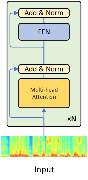
Although LSTM can capture short-term dependencies, Transformer is much better at capturing long-term dependencies because its attention mechanism sees all context directly. Transformer was shown to outperform LSTM zeyer2019comparison ; karita2019comparative ; li2020comparison and is now replacing LSTM in all E2E models dong2018speech ; karita2019comparative ; zeyer2019comparison ; zhang2020transformer ; li2020comparison ; higuchi2020mask . The encoder of Transformer-based E2E models is composed of a stack of Transformer blocks, where each block has a multi-head self-attention layer and a feed-forward network (FFN), as shown in Figure 5(a). Residual connections he2016deep and layer normalization ba2016layer are used to connect different layers and blocks. The input of a Transformer block can be linearly transformed to the query , key , and value vectors with matrices , , and , respectively. Self-attention is used to compute the attention distribution over the input speech sequence with the dot-product similarity function as
| (12) | |||||
where is a scaling factor and is the dimension of the feature vector for each head. Then, the attention weights are used to combine the value vectors to generate the layer output at the current time step
| (13) |
Multi-head self-attention (MHSA) is used to further improve the model capacity by applying multiple parallel self-attentions on the input sequence and the outputs of each attention module are then concatenated. By replacing the LSTM modules with Transformer in the encoder, the RNN-T model becomes Transformer Transducer yeh2019transformer ; zhang2020transformer ; chen2021developing ; dalmia2021transformer which has better accuracy than RNN-T due to the modeling power of Transformer.
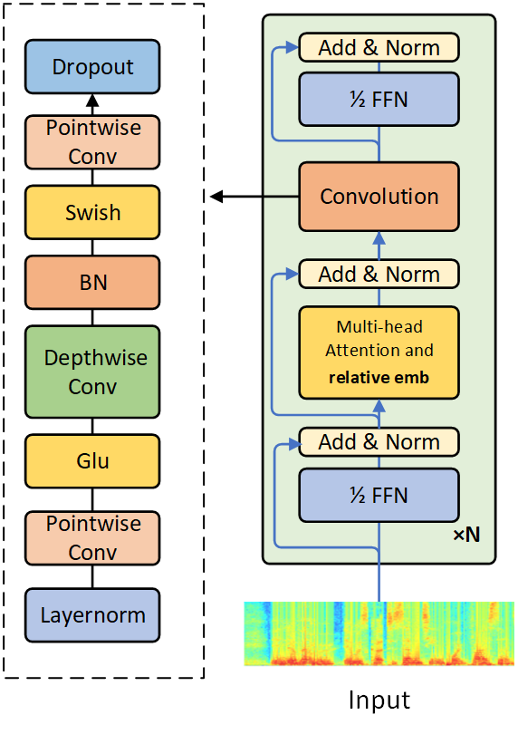
While Transformer is good at capturing global context, it is less effective in extracting local patterns. To further improve the modeling capability, convolutional neural network (CNN) waibel1989phoneme ; lecun1989backpropagation which works on local information is combined with Transformer as Conformer gulati2020conformer which is plotted in Figure 5(b). The conformer block contains two half-step FFNs sandwiching the MHSA and convolution modules. Although having higher model complexity than Transformer, Conformer has been reported to outperform Transformer in various tasks gulati2020conformer ; guo2021recent .
Again, the self-attention on the full speech sequence cannot be used for streaming ASR. In chen2021developing , a masking strategy was proposed to flexibly control how attention is performed. A binary attention mask is introduced to the self-attention in Eq. (12) as
| (14) | |||||
Figure 6 shows several examples of how the binary mask is used for different computational costs and latency configurations when predicting the output for . The full attention case is plotted in Figure 6(a), where the reception field is the full sequence, and every element of the mask matrix is . For the strict streaming setup without any latency, the attention should not be performed on any future frame, as shown in Figure 6(b). The major drawback of this attention mechanism is that the memory and runtime cost increases linearly as the utterance history grows. The context operation zhang2020transformer was proposed to address the issue by working on a limited history at every layer. Shown in 6(c), because of context expansion, the model still can access a very long history. If the attention operates on history frames at every layer and the model has Transformer layers, then the model can access history frames. In order to improve modeling accuracy, it is better to also include some future frames into the prediction. In zhang2020transformer , the same context expansion strategy is applied to not only the history but also the future frames. However, because of context expansion, it needs a large amount of future frames when there are many Transformer layers, introducing significant latency. A better future access strategy was proposed in chen2021developing ; shi2021emformer where the input speech sequence is segmented into fixed-size chunks. The frames in the same chunk can see each other and each frame can see fixed numbers of the left chunks so that the left reception field propagates. Plotted in Figure 6(d), this strategy helps to build high accuracy models with a very small latency. In addition to these methods, there are lots of variations tsunoo2019transformer ; moritz2020streaming ; wang2020low ; tian2020synchronous ; zhang2020streaming ; huang2020conv of localizing full self-attention in order to have a streaming Transformer encoder.
Another popular method is Gaussian soft-mask sperber2018self which changes the softmax calculation in self-attention in Eq. (12) as
| (15) |
where is a mask. It can be either a hard mask which sets all weights outside the band to 0 as
| (16) |
or a soft mask as
| (17) |
where is a trainable parameter. While both masks can enforce the locality which is good for the speech signal, the soft-mask method cannot reduce computational cost and latency because it sill attends the full sequence, although the weights of far-away time steps are small.


4 Other Training Criterion
In addition to the standard training loss for E2E models, there are other losses used in the popular teacher-student learning and minimum word error rate training.
4.1 Teacher-Student Learning
The concept of teacher-student (T/S) learning was originally introduced in bucilua2006model but became popular from the deep learning era. The most popular T/S learning strategy is to minimize the KL divergence between the output distributions of the teacher and student networks, first proposed in 2014 by Li et al. li2014learning . Later, Hinton et al. hinton2015distilling branded it with a new name, knowledge distillation, by introducing a temperature parameter (like chemical distillation) to scale the posteriors.
In the context of E2E modeling, the token-level loss function of T/S learning is
| (18) |
where and denote the posterior distributions of the teacher and student networks, respectively. The most popular usage of T/S learning in E2E modeling is to learn a small student E2E model from a large teacher E2E model li2018developing ; pang2018compression ; kim2019knowledge ; panchapagesan2021efficient .
Another usage is to learn a streaming E2E model from a non-streaming E2E model kim2018improved ; kurata2019guiding ; moriya2020distilling ; kurata2020knowledge ; kojima21knowledge . It is a little tricky here because the streaming E2E models usually generate delayed decisions. For example, the streaming CTC and non-streaming CTC have different output spike patterns. Therefore, delicate work has been done in order to make the non-streaming E2E models generate friendly output spikes that can be learned by the streaming E2E models kurata2019guiding ; kurata2020knowledge . Another way to circumvent the spike mismatch is to train the streaming E2E model by using the ASR hypotheses generated from decoding the unlabeled data with a non-streaming E2E model doutre2021improving .
T/S learning can also be used to adapt an E2E model from a source environment to a target environment if the target-domain acoustic data can be paired with the source-domain acoustic data either by recording at the same time or from simulation meng2019domain ; zhang2019knowledge . The loss function in Eq. (18) is re-written as
| (19) |
While standard T/S learning follows a two-step process in which we first train a teacher model and then use the T/S criterion to train a student model, there are recent studies wu2021dynamic ; yu2021dual ; swaminathan2021codert ; nagaraja2021collaborative that train the teacher and student models at the same time. Such a co-learning strategy not only simplifies the training process but also boosts the accuracy of student models.
4.2 Minimum Word Error Rate Training
The minimum word error rate (MWER) training criterion tries to mitigate the discrepancy between the training criterion and the evaluation metric of a speech recognition model. Instead of minimizing the negative log loss of the probability , MWER minimizes the expected word errors shannon2017optimizing as
| (20) |
where denotes the posterior probability of an hypothesis , denotes the risk function which measures the edit-distance between the hypothesis and the reference transcription at word-level. While the exact posterior probability is computationally intractable, in practice, an N-best list of hypotheses from beam search decoding are used to compute the empirical posterior probability prabhavalkar2018minimum as
| (21) |
where is the probability of an hypothesis , computed in Eq. (4) for AED models or Eq. (8) for RNN-T models.
MWER has been shown to improve the accuracy of AED models prabhavalkar2018minimum ; cui2018improving , RNN-T models weng2020minimum ; guo2020efficient , and hybrid autoregressive transducer (HAT) models lu2021on . However, the gain is not as significant as what has been reported in hybrid models. One possible reason is that the MWER training of hybrid models follows the cross-entropy training which is frame-based. In contrast, E2E models have already been optimized with sequence-level training, therefore further sequence-level MWER training gives less gain.
5 Multilingual modeling
Building a multilingual ASR system with traditional hybrid models is difficult because every language usually has its own language-specific phonemes and word inventories. Most hybrid multilingual works focus on building an acoustic model with shared hidden layers huang2013cross ; heigold2013multilingual ; ghoshal2013multilingual , while every language has its own lexicon model and language model. In contrast, it is very easy to build a multilingual E2E ASR system by simply taking a union of the token (e.g., character, subword, or even byte) sets of all languages as the output token set and then training an E2E model with all the data watanabe2017language ; kim2018towards ; toshniwal2018multilingual ; cho2018multilingual ; li2019bytes . Such an E2E model is a universal ASR model which is capable of recognizing the speech from any language as long as that language has been used during training. However, pooling all languages together to train a multilingual model is a double-edged sword. Although it is simple and maximizes the sharing across languages, it also brings confusion between languages during recognition.
If the multilingual model can condition on the language identity (LID), significant improvement can be obtained over the universal multilingual model without LID because the one-hot LID guides the ASR model to generate the transcription of the target language by reducing the confusion from other languages toshniwal2018multilingual ; li2018multi ; kannan2019large ; zhu2020multilingual ; pratap2020massively ; sun2021improving . However, such a multilingual E2E model with LID relies on the prior knowledge of which language the user will speak for every utterance, working more like a monolingual model. To remove the dependency on knowing one-hot LID in advance, one way is to estimate the LID and use it as the additional input to E2E multilingual models. However, the gain is very limited, especially for streaming E2E models, because the estimation is not very reliable waters2019leveraging ; punjabi2020streaming .
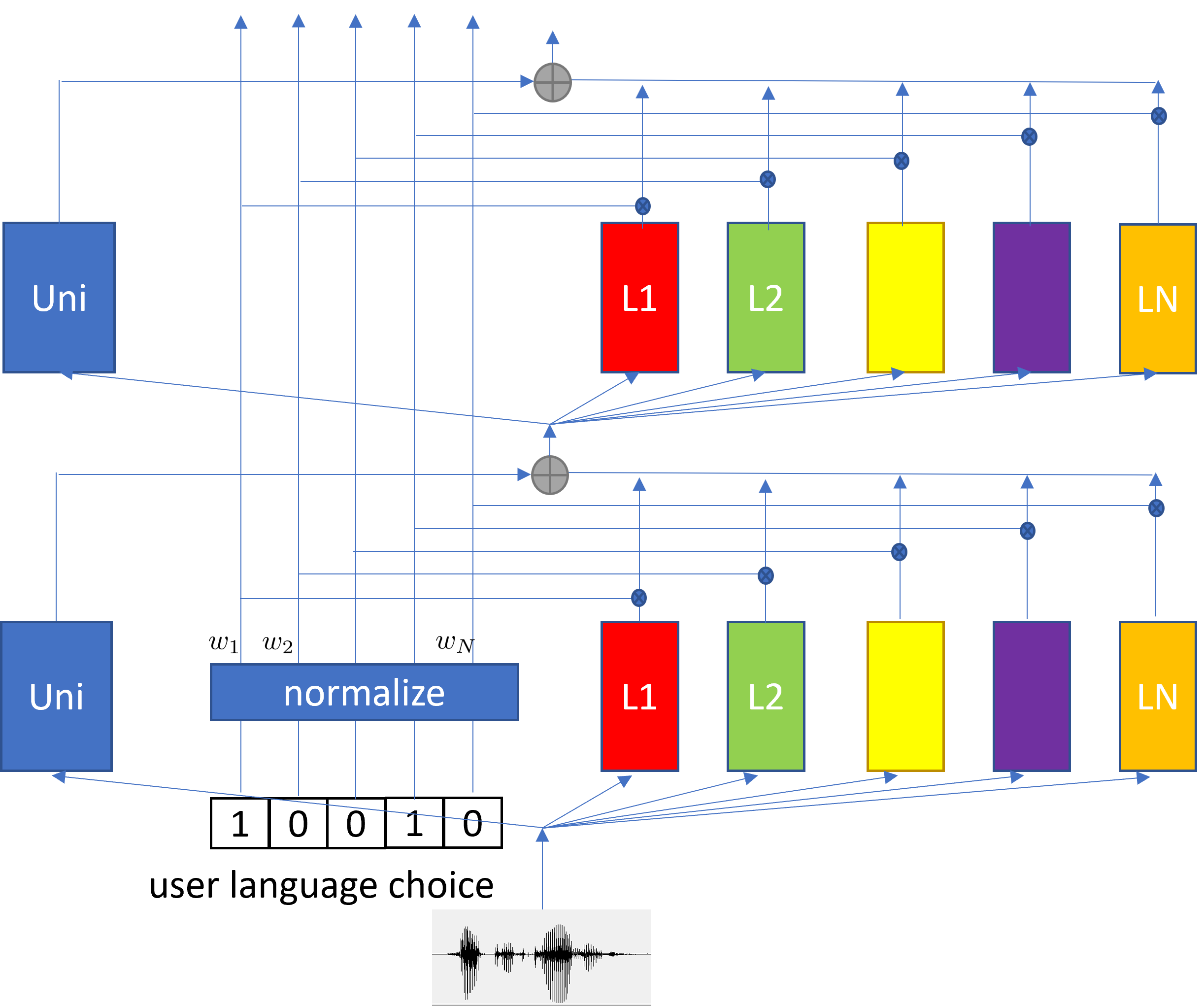
Because there are more multilingual users than monolingual users multilingual , there is an increasing demand of building multilingual systems which can recognize multiple languages without knowing in advance which language each individual utterance is from. One solution is to build a corresponding multilingual E2E model for any set of language combinations. However, this is impractical because the number of possible language combinations is huge given so many languages in the world. Zhou et al. proposed a configurable multilingual model (CMM) zhou2022configurable which is trained only once by pooling the data from all languages, but can be configured to recognize speeches from any combination of languages. As shown in Figure 7, the hidden output of CMM is calculated as the weighted sum of the output from a universal module and the outputs from all language-specific modules. At runtime, the universal module together with corresponding language-specific modules are activated based on the user choice. Because multilingual users usually speak a few languages, CMM reduces the language confusion space from dozens to a few. Therefore, it performs much better than the multilingual model without LID, and can serve the multilingual users well.
There are several factors to be considered when designing multilingual E2E models. When scaling the multilingual model to cover a large amount of languages (e.g., 50 languages in pratap2020massively ), the data from those languages is heavily imbalanced, which usually leads to a model performing well on resource-rich languages while failing on low-resource languages. To solve that issue, data sampling is usually used to balance the training data amount kannan2019large ; pratap2020massively . The model capacity should also be expanded to recognize a large amount of languages. In pratap2020massively ; li2021scaling , multilingual models are scaled to billions of parameters.
Because there are differences across languages, it may not be optimal if a simple E2E structure is used to blindly model all the multilingual data. In kannan2019large , language-specific adapt layers are used to further boost the multilingual model performance. Similar ideas are used with the mixture of expert structure for multilingual models das2021multi ; gaur2021mixture .
While E2E models have achieved remarkable success in multilingual modeling, an even more challenging topic is the ASR of code-switching (CS) utterances which contain mixed words or phrases from multiple distinct languages. There are two categories of CS: one is intra-sentential CS where switches happen within an utterance and the other is inter-sentential CS where switches occur between utterances with monolingual words inside each utterance. The former one is more difficult, attracting most studies. In seki2018end , synthetic utterance-level CS text was generated to improve the AED model’s ASR accuracy on inter-sentential CS utterances. The challenge of intra-sentential CS to E2E models was addressed in li2019towards by using the LID model to linearly adjust the posterior of a CTC model, followed by lots of recent studies (e.g., khassanov2019constrained ; yue2019end ; lu2020bi ; qiu2020towards ; nj2020investigation ; dalmia2021transformer ; zhang2021rnn ; diwan2021multilingual ). One major challenge to CS ASR is the lack of the CS data while E2E models are more data hungry. Therefore, methods have been studied to effectively leverage monolingual data. A constrained output embedding method khassanov2019constrained was proposed to encourage the output embedding of monolingual languages similar in order to let the ASR model easily switch between languages. In lu2020bi ; dalmia2021transformer , a bi-encoder which has a separate encoder for each language is used to train the model from monolingual data. This was further extended with both language-specific encoder and language-specific decoder to recognize CS speech zhou2020multi .
6 Adaptation
The performance of ASR systems can degrade significantly when the test conditions differ from training. Adaptation algorithms are designed to address such challenging issues. A comprehensive overview of adaptation technologies in ASR can be found in bell2020adaptation . In this section, we highlight some adaptation technologies for E2E models.
6.1 Speaker Adaptation
Speaker adaptation adapts ASR models to better recognize a target speaker’s speech. It is a common practice to adapt the acoustic encoder of CTC li2018speaker ; do2021multiple , AED weninger2019listen ; meng2019speaker , RNN-T sim2019personalization ; huang2020rapid and Conformer Transducer huang2021rapid . Another popular methodology is to augment the input speech with speaker embeddings delcroix2018auxiliary ; sari2020unsupervised ; zhao2020speech .
The biggest challenge of speaker adaptation is that the adaptation data amount from the target speaker is usually very small. There are several ways to address such a challenge. The first one is using regularization techniques such as Kullback-Leibler (KL) divergence regularization yu2013kl , maximum a posteriori adaptation huang2015maximum , or elastic weight consolidation kirkpatrick2017overcoming , to ensure the adapted models do not overfit the limited adaptation data li2018speaker ; sim2019personalization ; weninger2019listen ; meng2019speaker . The second approach is multi-task learning. E2E models typically use subword units as the output target in order to achieve high recognition accuracy. Sometimes, the number of subword units is at the scale of thousands or even more. These units usually cannot be fully observed in the limited speaker adaptation data. In contrast, the small number of character units usually can be fully covered. Therefore, multi-task learning using both character and subword units can significantly alleviate such sparseness issues li2018speaker ; meng2019speaker . The third approach is to use multi-speaker text-to-speech (TTS) to expand the adaption set for the target speaker sim2019personalization ; huang2020rapid . Because the transcription used to generate the synthesized speech is also used for model adaptation, this approach also alleviates the hypothesis error issue in unsupervised adaptation when combining the synthesized speech with the original speech from the target speaker.
It is desirable to use E2E models on devices because of the compact model size. There are interesting works sim2019investigation ; sim2021robust which study how to do secure adaptation on devices with continuous learning so that the user data never leaves devices. Several engineering practices were described in order to deal with the limited memory and computation power on devices.
6.2 Domain Adaptation
Domain adaptation is the task of adapting ASR models to the target domain which has content mismatch from the source domain in which the ASR models were trained. Because E2E models tend to memorize the training data well, their performance usually degrades a lot in a new domain. Such a challenge attracts much more works on domain adaptation than speaker adaptation. This is not a severe issue for hybrid models because their language model (LM) is trained with a much larger amount of text data than that is used in the paired speech-text setup for E2E model training. The big challenge of adapting E2E models to a new domain is that it is not easy to get enough paired speech-text data in the new domain, which requires transcribing the new-domain speech. However, it is much easier to get text data in the new domain. Therefore, the mainstream of domain adaptation methods for E2E models focuses on the new-domain text only.
A widely adopted approach to adapt E2E models to a new domain is fusing E2E models with an external LM trained with the new-domain text data. There are several LM fusion methods, such as shallow fusion gulcehre2015Shallow , deep fusion gulcehre2015Shallow , and cold fusion Sriram2018Cold . Among them, the simplest and most popular method is shallow fusion in which the external LM is log-linearly interpolated with the E2E model at inference time toshniwal2018comparison .
However, shallow fusion does not have a clear probabilistic interpretation. As an improvement, a maximum a posteriori based decoding method kanda2016maximum ; kanda2017maximum was proposed for the integration of an external LM for CTC. A density ratio approach based on Bayes’ rule was proposed in mcdermott2019density for RNN-T. During inference, the output of the E2E model is modified by the ratio of the external LM trained with the new-domain text data and the source-domain LM trained with the transcript of the training set which has the paired speech-text data for E2E model training. Another similar model is the hybrid autoregressive transducer (HAT) model variani2020hybrid designed to improve the RNN-T model. In the HAT model, the label distribution is derived by normalizing the score functions across all labels excluding blank. Hence, it is mathematically justified to integrate the HAT model with an external LM using the density ratio method.
In meng2021internal , an internal LM estimation (ILME)-based fusion was proposed to enable a more effective LM integration. During inference, the internal LM score of an E2E model is estimated by zeroing out the contribution of the encoder and is subtracted from the log-linear interpolation between E2E and external LM scores. An internal LM training (ILMT) method meng2021ILMT was further proposed to minimize an additional internal LM loss by updating only the components that estimate the internal LM. ILMT increases the modularity of the E2E model and alleviates the mismatch between training and ILME-based fusion.
Tuning the LM weights on multiple development sets is computationally expensive and time-consuming. To eliminate the weights tuning, the MWER training with LM fusion was proposed in peyser2020improving ; meng2021minimum where the LM fusion is performed during MWER training. During inference, LM weights pre-set in training enables a robust LM fusion on test sets from different domains.
Because LM fusion methods require interpolating with an external LM, both the computational cost and footprint are increased, which may not be applicable to ASR on devices. With the advance of TTS technologies, a new trend is to adapt E2E models with the synthesized speech generated from the new-domain text sim2019personalization ; peyser2019improving ; Li2020Developing ; zheng2021using . This is especially useful for adapting RNN-T, in which the prediction network works similarly to an LM. It was shown that such domain adaptation method with TTS is more effective than LM fusion methods Li2020Developing .
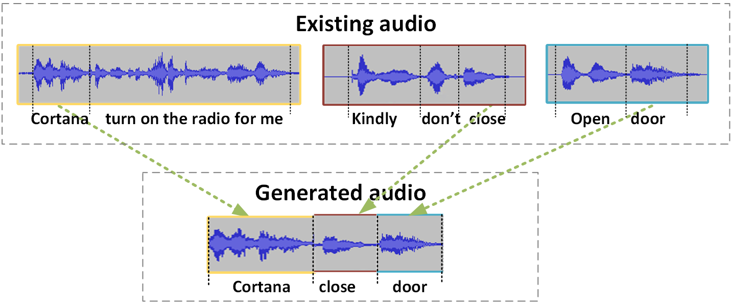
The TTS-based adaptation method also has its drawbacks. The first is that TTS speech is different from the real speech. It sometimes also degrades the recognition accuracy on real speech li2019semi . This issue was alleviated in kurata2021improving by inserting a mapping network before the encoder network when the input is TTS audio in both the training and adaption stage. This mapping network works as feature space transformation to map the space of TTS audio to the space of real speech. During testing with real speech, the mapping network was removed. The second is that the speaker variation in the TTS data is far less than that in the large-scale ASR training data. The third is the cost of training a multi-speaker TTS model and the generation of synthesized speech from the model is large. These issues were solved by a spliced data method zhao2021addressing which was used to adapt E2E models with better performance than the TTS-based adaptation method. For any text sentence in the new domain, the method randomly extracts the corresponding audio segments from the source training data, and then concatenates them to form new utterances. Figure 8 gives an example of how this spliced data method works. Similar ideas have been used for data augmentation by replacing some word segments in an utterance with new word segments from another utterance to train a general E2E model sun2021semantic ; lam2021fly .
Both the TTS-based adaptation and the spliced data method need to synthesize audios from text, and then update E2E models. Recently, a fast text adaptation method pylkkonen2021fast was proposed to adapt the prediction network of RNN-T by treating it as an LM and then using the text from the new domain to update it. In meng2021internal2 , ILMT meng2021ILMT was used to ensure that the internal LM inside RNN-T behaves similarly to a standalone neural LM, and then it can be adapted with text only data.
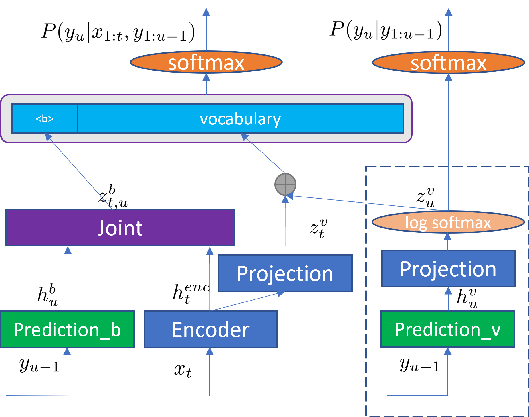
However, as shown in ghodsi2020rnn , the prediction network in RNN-T does not fully function as an LM. Chen et al. showed this is because the prediction network needs to predict both normal tokens and blank, and therefore proposed a factorized neural transducer which separates the prediction of normal tokens and blank chen2021factorized . As shown in Figure 9, the modules in the dashed box function exactly as an LM, predicting the probability . Therefore, it can be updated with the text from the new domain by using any well-established neural LM adaptation methods. Finally, the adapted factorized neural transducer with the branch output is used to recognize the speeches from the new domain with large accuracy improvement chen2021factorized .
While these domain adaptation technologies are powerful, it is desirable that the adaptation of E2E models to the new domain does not degrade the models’ performance on the source domain. Therefore, it is worth looking at the concept of lifelong learning which enables E2E models to learn new tasks without forgetting the previously learned knowledge chang2021towards . If the source-domain data is available, it can be mixed with the new-domain data for adaptation zhao2021addressing . Otherwise, the popular solution is to use regularization that prevents the adapted model from moving too far away from the source model meng2021internal2 .
6.3 Customization
Different from speaker adaptation which adjusts a speaker independent E2E model toward the speaker audio and domain adaptation which lets an E2E model recognize the content of a new domain better, customization here specifically refers to the technologies that leverage context such as contacts, location, music playlist etc., of a specific user to significantly boost the ASR accuracy for this user. For example, an English ASR system usually cannot recognize the contact names of a Chinese person well. However, if the English ASR system is presented with the contact list of this Chinese person, the ASR output can be biased toward the contact names. Such biasing is even more effective when designed with context activation phrases such as "call", "email", "text", etc.
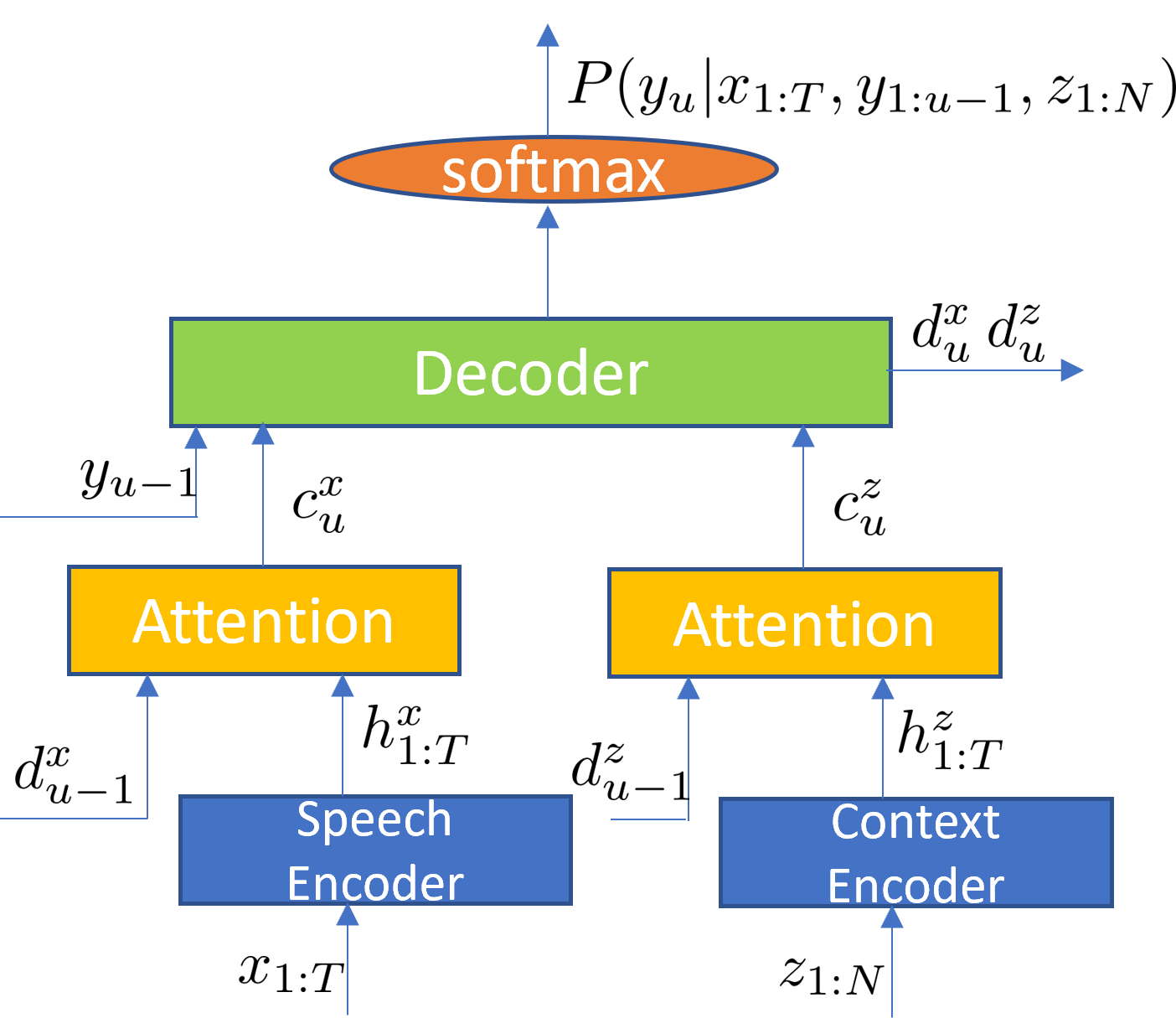
While it is relatively easier for hybrid systems to do so with the on-the-fly rescoring strategy which dynamically adjusts the LM weights of a small number of n-grams which are relevant to the particular recognition context, it is more challenging to E2E systems. One solution is to add a context bias encoder in addition to the original audio encoder into the E2E model, which was first proposed in he2017streaming to bias a keyword spotting E2E model toward a specific keyword. The idea was then extended into a contextual LAS (CLAS) ASR model pundak2018deep , plotted in figure 10. LAS (Listen, Attend and Spell) chan2016listen is one particular instantiation of AED. Compared to the standard AED model in figure 1(b), CLAS adds the context encoder in the bottom right of the figure which takes the context list as the input, where denotes the -th phrase. An attention module is used to generate the contextual vector as one of the inputs to the decoder. In this way, the network output conditions not only on the speech signal and previous label sequence but also on the contextual phrase list. It was further extended into a two-step memory enhanced model in huber2021instant . It is common that a contextual phrase list contains rare words, especially names which are not observed during training. In such a case, E2E models have not learned to map the rare words’ acoustic signal to words. This issue can be alleviated by further adding a phoneme encoder in addition to the text encoder for the contextual phrase list bruguier2019phoebe ; chen2019joint . The same idea has also been applied to RNN-T jain2020contextual .
However, as shown in pundak2018deep , it becomes challenging for the bias attention module to focus if the biasing list is too large (e.g., more than 1000 phrases). Therefore, a more popular way to handle a large contextual phrase list is shallow fusion with the contextual biasing LM zhao2019shallow ; le2021deep . A challenge for the fusion-based biasing method is that it usually benefits from prefix which may not be available all the time. In huang2020class , class tags are inserted into word transcription during training to enable context aware training. During inference, class tags are used to construct contextual bias finite-state transducer. In le2021contextualized , trie-based deep biasing, WFST shallow fusion and neural network LM contextualization are combined together to reach good biasing performance for tasks with and without prefix. As discussed in Section 6.6.2, density ratio and HAT perform better than shallow fusion when integrating an external LM. Contextual biasing with density ratio and HAT were also shown to have better biasing performance andres2021contextual ; sainath2021efficient .
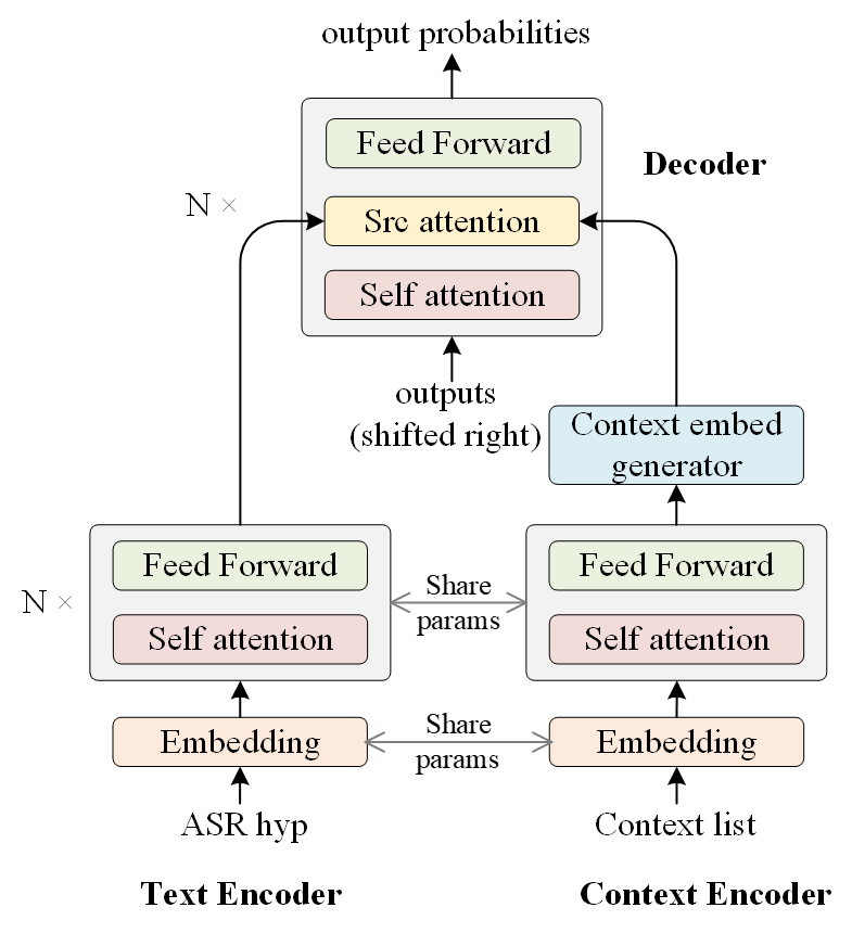
The most challenging part of context biasing is how to deal with a very large bias list which contains more than 1000 phrases. Wang et al. wang2021a provided a nice solution by extending spelling correction guo2019spelling to contextual spelling correction (CSC), which is shown in Figure 11. Both the embeddings of the ASR hypothesis and the contextual phrase list are used as the input to the decoder, which generates a new word sequence. A filtering mechanism based on the distance between ASR hypothesis and contextual phrases is used to trim the very large phrase list to a relatively small one so that the attention can perform well. Such filtering is the key to the success which cannot be done inside ASR models such as CLAS because the filtering relies on the ASR decoding results.
7 Advanced Models
In this section, we discuss several advanced models.
7.1 Non-Autoregressive Models
While most E2E models use autoregressive (AR) modeling to predict target tokens in a left-to-right manner as Eqs. (4), there is a recent trend of using non-autoregressive (NAR) modeling which generates all target tokens simultaneously with one-shot or iteratively without replying on predicted tokens in early steps higuchi2020mask ; bai2020listen ; tian2020spike ; chen2020non ; song2021non ; fan2021cass ; higuchi2021improved . These NAR methods root from the assumption that the feature sequence generated by the acoustic encoder contains not only acoustic information but also some language semantic information. However, such an assumption is not very strong, resulting in worse performance of NAR modeling compared to AR modeling in general. The biggest advantage of NAR models is that its decoding speed is much faster than that of AR models because there is no dependency on previous tokens. All target tokens can be predicted in parallel while the decoding of AR models is more complicated because of the token dependency.
A typical way to generate all target tokens is described in bai2020listen . The target token sequence length is predicted or set as a constant value. Then the NAR model assumes that each token is independent of each other as
| (22) |
At decoding time, the predicted token at each position is the one with the highest probability.
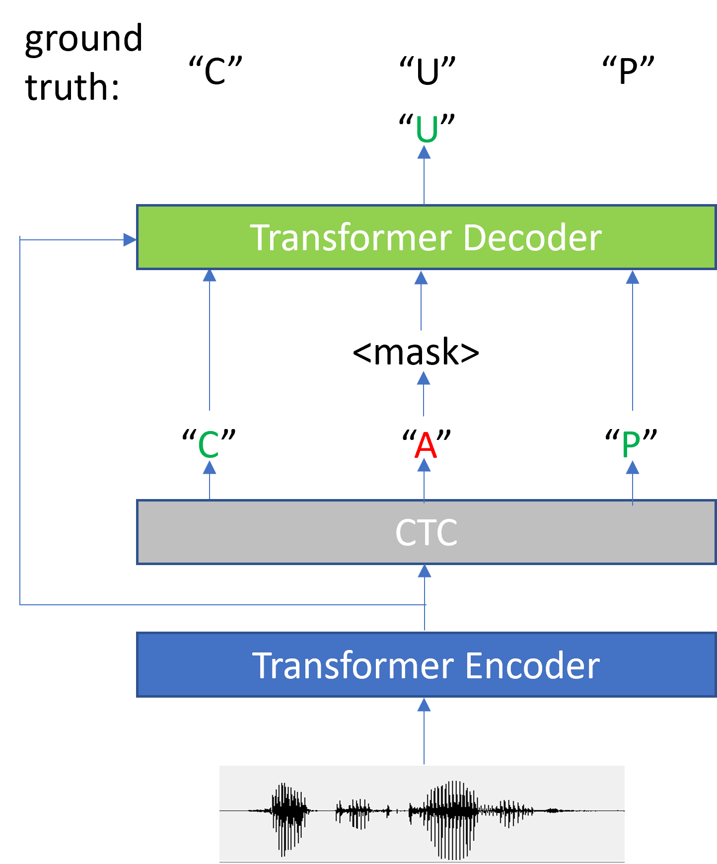
The independence assumption in Eq. (22) is very strong. The token sequence is also hard to predict usually. Mask CTC higuchi2020mask was proposed to solve these issues. It predicts a set of masked tokens , conditioning on the observed tokens and the input speech sequence as
| (23) |
Figure 12 shows an example of how Mask CTC works. The target sequence was first initialized with the CTC outputs. Then tokens with low confidence scores are masked and are iteratively optimized conditioning on the unmasked tokens and input speech sequence. The length of the final token sequence generated by Mask CTC is the same as the length of the CTC initial output, therefore Mask CTC can only deal with the substitution error. In higuchi2021improved , the length of a partial target sequence is predicted to enable Mask CTC’s ability of handling deletion and insertion errors.
7.2 Unified Models
The most significant component in E2E models is the encoder, which is well studied in literature. There are lots of encoder designs depending on the requirements of streaming, latency, and computational cost in different target scenarios. The development cost is formidable if we train a separate E2E model for each application scenario. Therefore, an emerging trend is to train a single unified model which can be configured with multiple streaming, latency, and computational cost setups during decoding. In yu2021dual , a dual E2E model was proposed with shared weights for both streaming and non-streaming ASR. In order to have a dual-mode Conformer encoder, the authors designed dual-mode modules for the components such as convolution, pooling, and attention layers inside Conformer. An in-place T/S learning was used to train the student streaming mode from the full-context non-streaming mode. Such training even brought accuracy and latency benefits to the streaming ASR. Another model unifying streaming and non-streaming modes was proposed in audhkhasi2021mixture which decomposes the Transformer’s softmax attention into left-only causal attention and right-only anti-causal attention. For the streaming scenario, it just uses the causal attention while the non-streaming mode uses both attentions.
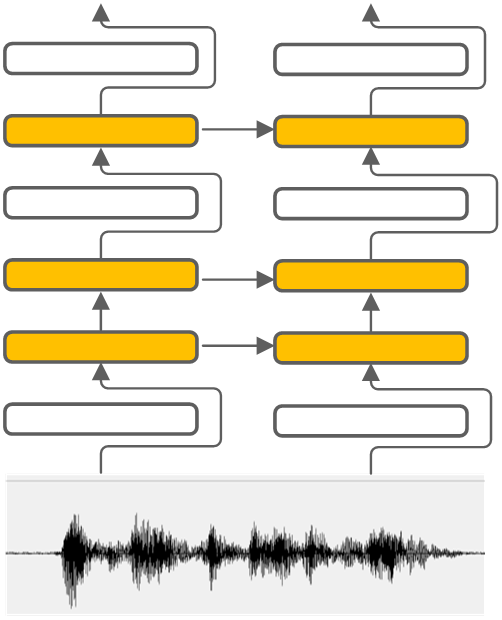
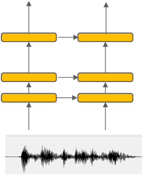
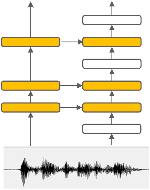
There are several studies working on a unified model with dynamic computational cost during inference. In wu2021dynamic , a dynamic sparsity network is used as the encoder of RNN-T. It only needs to be trained once and then can be set with any predefined sparsity configuration at runtime in order to meet various computational cost requirements on different devices. An even more direct way to have a dynamic encoder was proposed in shi2021dynamic . During training, layer dropout is applied to randomly drop out encoder layer as shown in Figure 13(a). The pruned model can be used to decode full utterances for constant low computational cost as shown in Figure 13(b). An example of advanced usage of the dynamic encoder is plotted in Figure 13(c), where the dynamic encoder is configured with a small number of layers in the beginning of the utterance, and then configured with full layers in the remaining. The idea of having different computational costs within an utterance was also studied in macoskey2021amortized for RNN-T. The model has a fast encoder and a slow encoder. An arbitrator is used to select which encoder should be used given an input speech frame.
It requires a small latency for applications such as voice search and command control, while the applications such as dictation and video transcription usually can afford a larger latency. Variable context training tripathi2020transformer ; mahadeokar2021flexi ; kim2021multi was proposed to build a unified model which can be configured for different latency requirements at runtime. During training, the Transformer encoder is provided with different right context lengths which correspond to different theoretic latency. In mahadeokar2021flexi , the alignment constraint method mahadeokar2021alignment was also used to flexibly set latency thresholds for different tasks. A task ID is used at runtime to configure the Transducer model with different encoder segments and latency.
7.3 Two-pass Models
Although a single E2E model can already achieve very good ASR performance, its performance can be further improved with a second-pass model. Spelling correction methods guo2019spelling ; Zhang2019 were proposed by using TTS data to train a separate translation model which is used to correct the hypothesis errors made by the first-pass E2E model. The spelling correction model is a pure text-to-text model without using the speech input. As E2E models need to be trained with paired speech-text data, the language modeling power is always a concern of E2E models. Wang et al. proposed a two-pass RNN-T model in which the first-pass RNN-T transcribes speech into syllables while the second-pass RNN-T converts syllable sequences into character sequences wang2021cascade . Because the second-pass RNN-T uses text instead of speech as input, therefore it can leverage a much larger amount of text data to build a more powerful capability for language modeling.
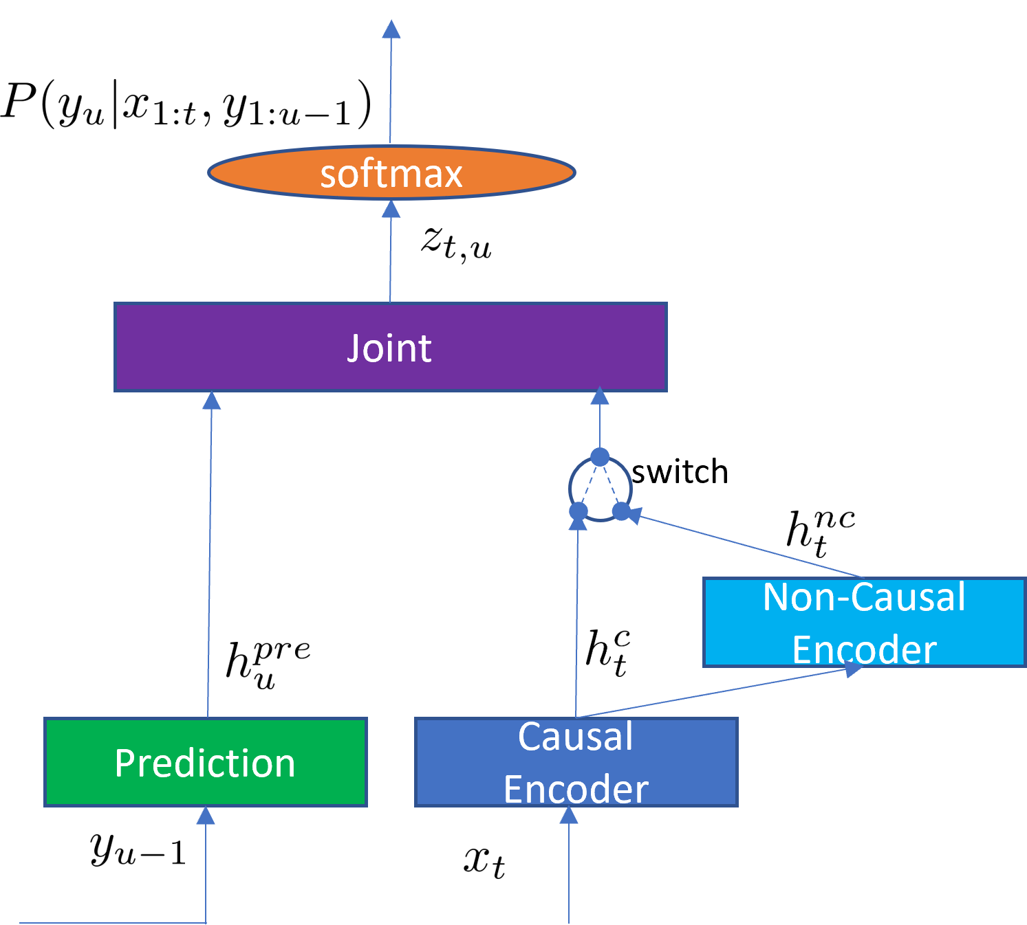
The second-pass processing with decoding hypothesis only cannot leverage the speech input. In sainath2019two , a two-pass model was proposed to use an AED decoder to attend the encoder output of a streaming RNN-T model. In this way, the first-pass RNN-T model provides immediate recognition results while the second-pass AED model can provide better accuracy with small additional perceived latency. This work was extended as the deliberation model which uses an LSTM AED decoder hu2020deliberation or a Transformer AED decoder hu2021transformer to attend both the encoder output and first-pass decoding hypothesis.
However, AED models cannot perform well on long utterances chiu2019comparison . Therefore, an RNN-T model with the cascaded encoder was proposed narayanan2021cascaded as shown in Figure 14. Such a model can also be considered as a unified model which provides both streaming and non-streaming solutions, and is a special case of Y-model tripathi2020transformer which has both streaming and non-streaming branches in a Y-shape. The causal encoder output is fed into a non-causal encoder to generate . Depending on applications, a switch is used to let or go to the joint network. In the context of two-pass modeling, the causal output is used in the first pass and the non-causal output is used in the second pass. Such a cascaded model is trained in one stage, while the first-pass and second-pass models in deliberation are trained in two stages. Another advantage of the RNN-T model with a cascaded encoder is its better performance on long utterances because the RNN-T decoder better handles long utterances than the AED decoder.
Note that the second-pass model brings additional latency and computational costs to ASR systems, therefore, careful designs have been studied to hide these costs in commercial systems chang2020low ; li2021better ; sainath2021efficient .
7.4 Multi-talker Models
While ASR systems have achieved very high recognition accuracy in most single-speaker applications, it is still very difficult to achieve satisfactory recognition accuracy in scenarios with multiple speakers talking at the same time. A common practice in the industry is to separate the overlapped speech first and then use an ASR model to recognize the separated speech streams yoshioka2019advances . The biggest challenge to multi-talker overlapping ASR is the permutation problem which occurs when the mixing sources are symmetric and the model cannot predetermine the target signal for its outputs. Deep clustering hershey2016deep and permutation invariant training (PIT) yu2017permutation were proposed to address such a challenge to separate overlapping speech signals. Specifically, PIT is simpler to implement and easier to be integrated with other methods. Therefore, it becomes the most popular speech separation method. Instead of the two-stage processing, Yu et al. yu2017recognizing proposed to directly optimize the ASR criterion with a single model using PIT without having an explicit speech separation step.
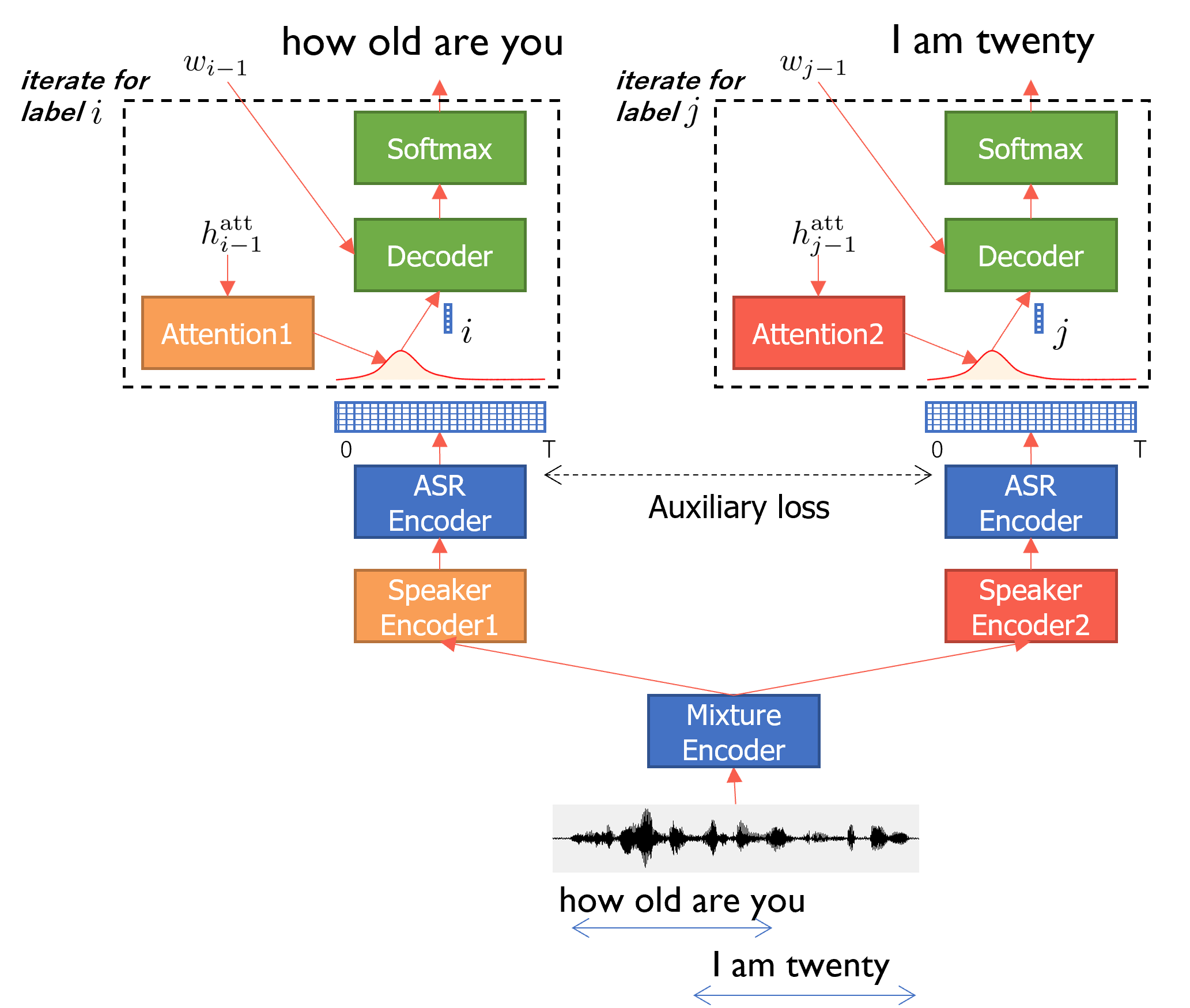
The first E2E model for overlapping speech was proposed in settle2018end with PIT loss in the label level without using the source signal from each speaker. It was further extended in chang2019end without pretraining, in chang2019mimo for multi-channel input and multi-channel output, and in chang2020end with Transformer. Figure 15(a) shows the network architecture of these methods. The overlapping speech goes through a mixture encoder for separation followed by two branches which generate the recognition results from two speakers. Most modules are shared between two branches except the attention module and speaker encoder. For the overlapping speech with speakers, the training loss is calculated by considering all possible speaker permutation as
| (24) |
where is the cross entropy function with the -th output and the permuted reference .
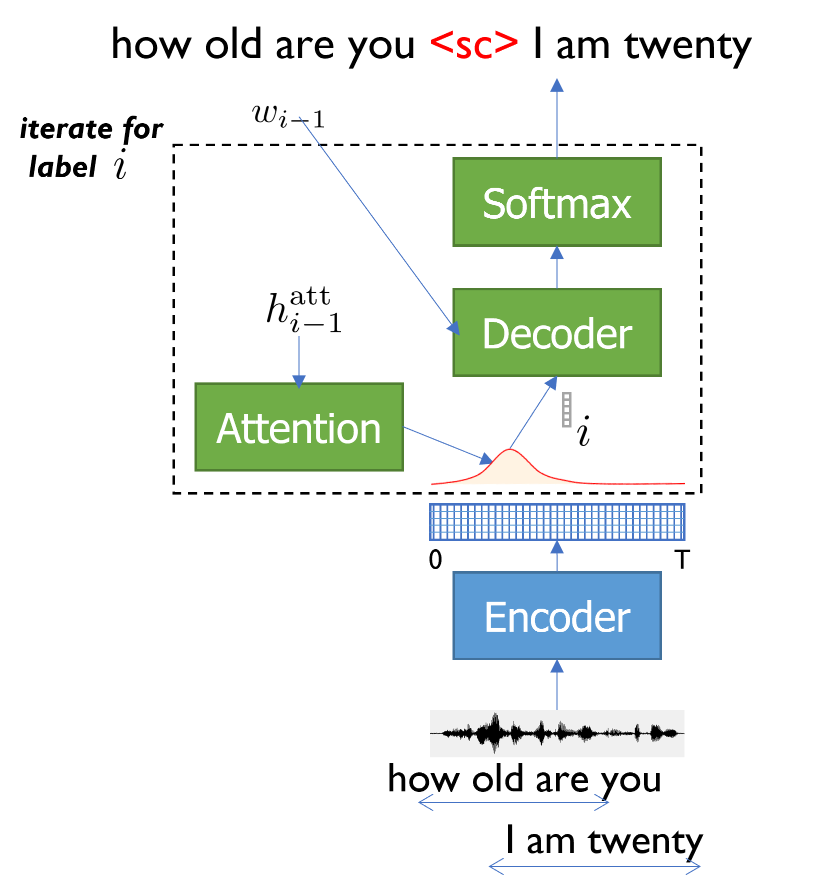
There are three theoretical limitations in the models with PIT-ASR loss in Eq (24). First, the number of output branches is the same as , the number of the speakers. After the model is trained, it cannot handle the overlapping speech with more speakers. Second, the training cost is using the Hungarian algorithm, which prevents it from being applied to scenarios with a large number of speakers. Third, there is possible leakage with duplicated decoding hypothesis between output branches because the outputs in different branches do not have a direct dependency. To address these limitations, Kanda et al. proposed a simple but effective serialized output training (SOT) method kanda2020serialized which uses a single AED model to predict the merged label sequence from all speakers as in Figure 15(b). A symbol is inserted between the reference label sequences of speakers to represent speaker change. Furthermore, the reference label sequences are ordered according to their start time in a first-in first-out manner. In this way, the training loss is significantly simplified as
| (25) |
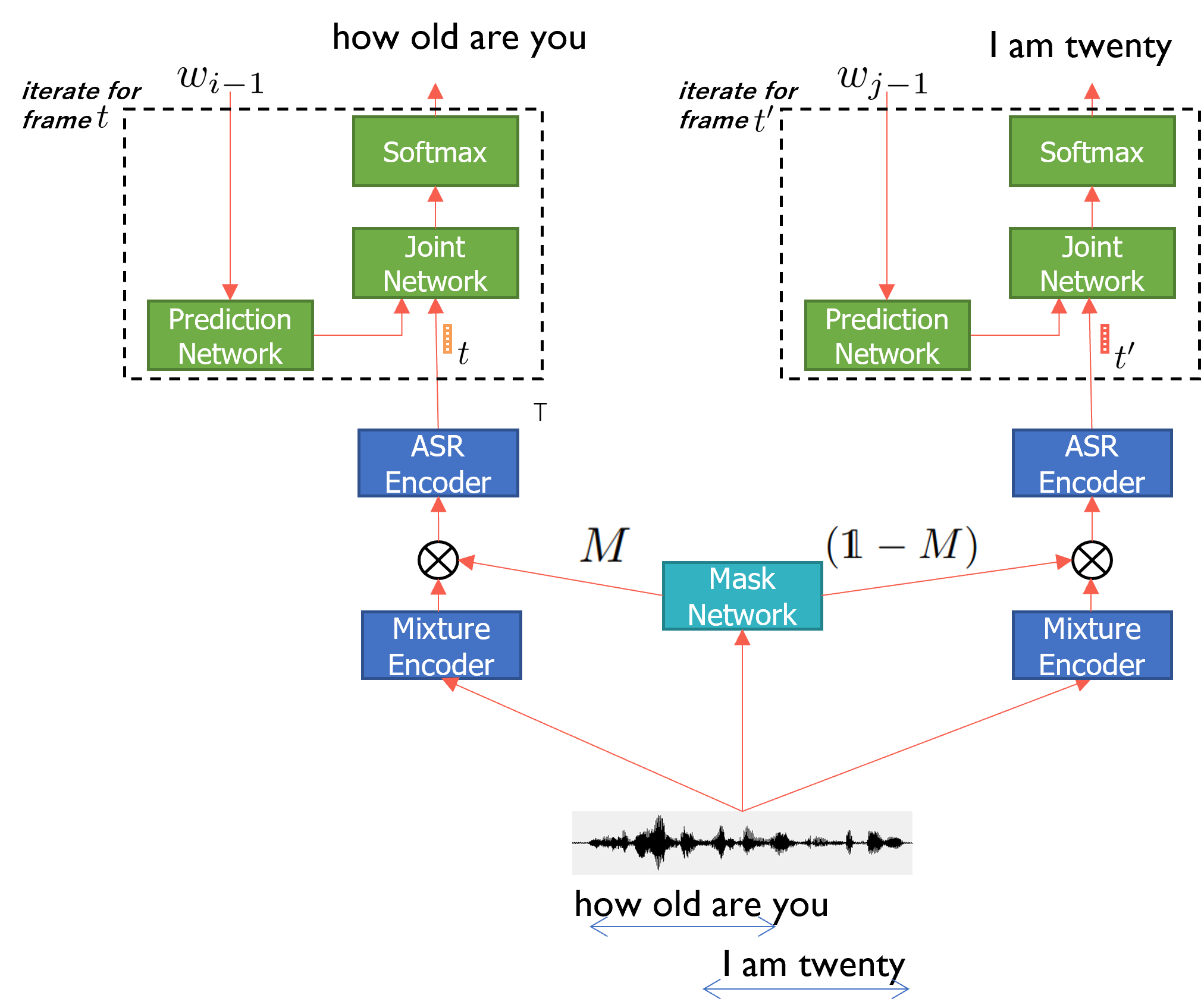
Given the large demand of streaming ASR in the industry, the backbone model of multi-talker ASR is also moving from the non-streaming AED model to the streaming RNN-T model. Although RNN-T was used in tripathi2020end for multi-talker ASR, it’s encoder is a bi-directional LSTM which is a non-streaming setting. In lu2021streaming ; sklyar2021streaming , the Streaming Unmixing and Recognition Transducer (SURT) was proposed as in Figure 15(c). A mask-based unmixing module is used to estimate masks in order to separate the speech input into two branches for recognition with RNN-T. Although PIT ASR loss in Eq. (24) can be used, it will introduce large computational cost due to the label permutation. Therefore, Heuristic Error Assignment Training (HEAT) lu2021streaming was proposed by ordering the label sequences based on the utterance start time into the set . The loss function can be written as
| (26) |
where stands for the -th element of . HEAT clearly reduces the training cost without losing accuracy lu2021streaming . It is even more important to use Eq. (26) in the continuous streaming setup where it is formidable to have all the permutations in a long conversation raj2022continuous .
7.5 Multi-channel Models
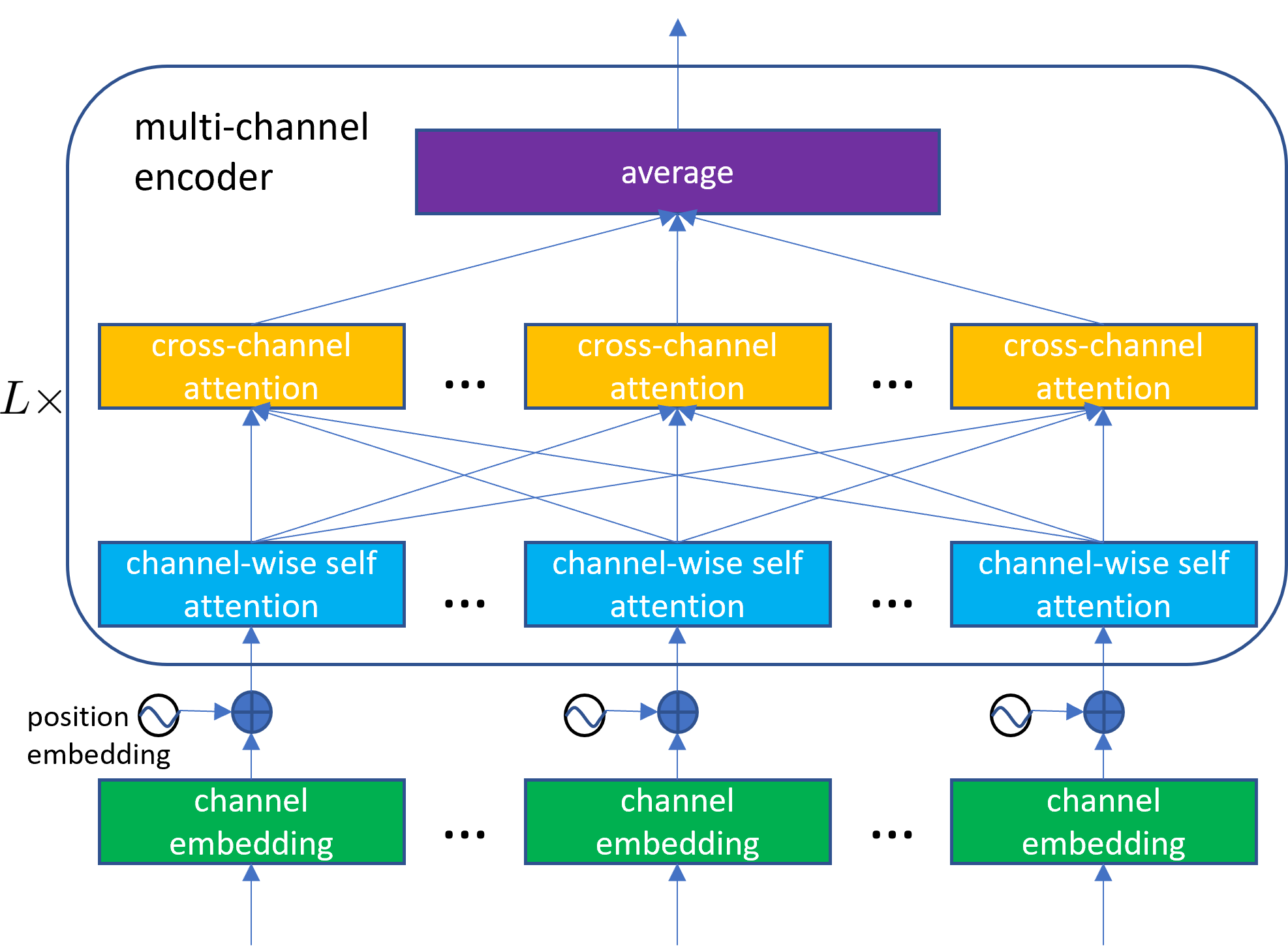
Beamforming is a standard technique for improving distant ASR system accuracy using microphone arrays with multi-channel inputs omologo2001speech ; kumatani2012microphone . The most popular beamforming technology for ASR is signal processing based superdirective beamforming, while there is a trend to replace it with the neural beamforming for joint optimization with the backend hybrid models heymann2016neural ; xiao2016deep ; sainath2017multichannel ; minhua2019frequency . The joint optimization is more direct when the backend model is an E2E model ochiai2017multichannel ; wang2021exploring , and can be applied with even more front end components zhang2020end ; zhang2021end . While all these methods still work on good neural beamforming modules, some recent studies try to bypass the beamforming module design by using a single E2E network to preform ASR directly on multi-channel inputs. Thanks to the power and flexibility of Transformer, the multi-channel Transformer ASR works chang2021end ; chang2021multi ; gong2021self replace the well-established beamformer with a multi-channel encoder which consumes the multi-channel inputs from microphone arrays. Figure 16 shows an example of a multi-channel encoder which consists of multiple blocks of cascaded within channel-wise self attention layer and cross-channel attention layer. The channel-wise self attention layer models the correlation across time within a channel while the cross-channel attention layer tries to learn the relationship across channels. The multi-channel encoder can then be plugged into any E2E model. Such E2E models do not need the conventional knowledge of beamformer design and were reported to perform better than the standard beamforming method followed by an ASR model chang2021end ; chang2021multi ; gong2021self .
8 Miscellaneous Topics
E2E modeling is a huge research topic. Due to the limit of space, we can only cover the most important areas we think about from the industry point of view. There are more areas worth mentioning. First of all, great toolkits doetsch2017returnn ; watanabe2018espnet ; wang2019espresso ; shen2019lingvo ; ravanelli2021speechbrain ; yao2021wenet are indispensable to the fast development of E2E ASR technologies. Among them, ESPnet watanabe2018espnet is the most popular E2E toolkit widely used in the speech community although some companies have their own in-house E2E model training tools. We will continue to witness the growth of E2E toolkits which benefit the whole speech community.
Model unit selection is a very important area in E2E modeling. While most units (characters hannun2014deep ; graves2014towards , word-piece schuster2012japanese ; chiu2018state ; zenkel2018subword ; xiao2018hybrid ; huang2019exploring , words soltau2016neural ; li2017acoustic ; audhkhasi2018building , or even phrases gaur2019acoustic ) are purely derived based on text and word-piece unit is the dominating one, there are also studies working on phoneme units sainath2018no ; irie2019model ; wang2020investigation ; zhou2021phoneme . As ASR is unique with the underlying acoustic signal, it should be better to build units bridging between the text and phoneme worlds. To that end, the pronunciation guided unit xu2019improving ; zhou2021acoustic ; papadourakis2021phonetically is worth studying.
Trained with paired speech-text data, E2E models are more data hungry than hybrid models. If the training data size is small, the performance of E2E models drops significantly. There are lots of ways to address the challenge of building E2E models for low-resource languages. First, regularization technologies such as dropout srivastava2014dropout can be used to prevent E2E models from overfitting to limited training data zhou2017improved . Data augmentation methods such as SpecAugment park2019specaugment and speed perturbation ko2015audio are also very helpful. In addition, there are also methods such as adversarial learning drexler2018combining and meta-learning hsu2020meta . The most popular solution is to first pre-train E2E models either with multilingual data or with self-supervised learning (SSL), and then fine-tune with the low-resource labeled data. A multilingual E2E model already captures lots of information across languages, which makes the transfer learning using the target language data very effective rosenberg2017end ; cho2018multilingual ; dalmia2018sequence ; inaguma2019transfer ; joshi2020transfer . SSL is even more powerful because it does not need any labeled data for pre-training, naturally solving the low-resource challenge. Therefore, SSL is becoming a new trend which especially works very well for ASR on resource limited languages schneider2019wav2vec ; chung2019unsupervised ; baevski2019vq ; baevski2020wav2vec ; chung2020generative ; zhang2020pushing ; wang2021unispeech ; hsu2021hubert , with representative technologies such as wav2vec 2.0 baevski2020wav2vec , autoregressive predictive coding chung2019unsupervised , and HuBERT hsu2021hubert . While most SSL studies focus on very limited supervised training data (e.g., 1000 hours), there are also recent studies showing promising results on industry-scale tens of thousand hours supervised training data wang2021unispeech2 ; zhang2021bigssl .
When training E2E ASR models, separate utterances are usually presented to the trainer. Therefore most ASR models are designed to recognize independent utterances. When the model is used to recognize a long conversation, a common practice is to segment the long conversation into utterances and then recognize them independently. However, the context information from previous utterances is useful to recognize the current utterance. In hori2020transformer ; hori2021advanced ; schwarz2021improving , audio and decoded hypotheses from previous utterances are concatenated as the additional input to the model when processing the current utterance.
When deploying E2E models to production, it is important to have an efficient decoding strategy, which was explored in saon2020alignment ; prabhavalkar2021less . Because the prediction network does not fully function as an LM as discussed in Section 6.6.2, the LSTM/Transformer in the RNN-T prediction network was recently replaced with a simple and cheap embedding with very limited context, which can be used to significantly reduce decoding cost and model size botros2021tied ; sainath2021efficient . When deployed to small-footprint devices, model compression pang2018compression ; mehrotra2020iterative ; panchapagesan2021efficient , quantization nguyen2020quantization ; fasoli20214 , and the combination of multiple technologies shangguan2020optimizing should be considered. Confidence measure and word timing are sometimes required for practical E2E systems. For example, in a video transcription system, confidence score is used to indicate which word may be recognized wrongly and then the user can listen to the video corresponding to that word using its timestamp. Examples of confidence measure work for E2E systems are oneactua2021evaluation ; li2021confidence ; qiu2021learning ; zhao2021addressing , and examples of word timing work for E2E systems are sainath2020emitting ; zhao2021addressing .
Almost all E2E models take Mel filter bank feature which is extracted from speech waveform as the input. In order to do the recognition really from end to end, speech waveform as the input to E2E models was studied in collobert2016wav2letter ; zeghidour2018end ; zeghidour2018fully ; parcollet2020e2e ; lam2021raw , especially in recent influential wav2vec series work schneider2019wav2vec ; baevski2020wav2vec . Because both E2E models and hybrid models have their own advantages and different error patterns, some works try to combine them together via rescoring li2019integrating , minimum Bayes’ risk combination wong2020combination , or two-pass modeling ye2022have . It is also very easy for E2E models to integrate inputs with multi-modality especially audio and visual signal together. There are plenty of works showing the benefits of visual signal for E2E ASR petridis2018end ; afouras2018deep ; petridis2018audio ; sterpu2018attention ; zhou2019modality ; tao2020end ; ghorbani2021listen ; ma2021end .
Robustness is always an important topic to ASR li2014overview . E2E models tend to fit training data and should have even severe robustness challenge due to the mismatch between training and testing. However, there is not too much activity in addressing such mismatch andrusenko2020towards ; prasad2021investigation . T/S learning was used to adapt a clean-trained E2E model to a noisy environment meng2019domain . Noise-invariant feature was learned to improve robustness in liang2018learning ; zhang2020learning . Data augmentation tsunoo2021data is another effective way to expose more testing environments to E2E models during training.
| work with key technologies | year | model | encoder | test-clean/other WER |
|---|---|---|---|---|
| Deep Speech 2: more labeled data, curriculum learning amodei2016deep | 2016 | CTC | bi-RNN | 5.3/13.2 |
| policy learning, joint training zhou2018improving | 2018 | CTC | CNN+bi-GRU | 5.4/14.7 |
| Shallow fusion, BPE, and pre-training zeyer2018improved | 2018 | AED | BLSTM | 3.8/12.8 |
| ESPRESSO recipe: lookahead word LM, EOS thresholding wang2019espresso | 2019 | AED | CNN+BLSTM | 2.8/8.7 |
| SpecAugment park2019specaugment | 2019 | AED | CNN+BLSTM | 2.5/5.8 |
| ESPnet recipe: SpecAugment, dropout karita2019comparative | 2019 | AED | Transformer | 2.6/5.7 |
| Semantic mask wang2019semantic | 2019 | AED | Transformer | 2.1/4.9 |
| Transformer-T, SpecAugment zhang2020transformer | 2020 | RNN-T | Transformer | 2.0/4.6 |
| Conformer-T, SpecAugment gulati2020conformer | 2020 | RNN-T | Conformer | 1.9/3.9 |
| wav2vec 2.0: SSL with unlabeled data, DataAugment baevski2020wav2vec | 2020 | CTC | Transformer | 1.8/3.3 |
| internal LM prior correction, EOS modelingzeyer2021librispeech | 2021 | RNN-T | BLSTM | 2.2/5.6 |
| w2v-BERT: SSL with unlabeled data, SpecAugment chung2021w2v | 2021 | RNN-T | Conformer | 1.4/2.5 |
| work with key technologies | year | model | encoder | test-clean/other WER |
|---|---|---|---|---|
| stable MoChA, truncated CTC prefix probability miao2019online | 2019 | AED | LC-BLSTM | 6.0/16.7 |
| triggered attention moritz2019streaming | 2019 | AED | time-delayed LSTM | 5.9/16.8 |
| triggered attention, restricted self-attention, SpecAugment moritz2020streaming | 2020 | AED | Transformer | 2.8/7.2 |
| Transformer-T, restricted self-attention, SpecAugment zhang2020transformer | 2020 | RNN-T | Transformer | 2.7/6.6 |
| scout network, chunk self-attention, SpecAugment wang2020low | 2020 | AED | Transformer | 2.7/6.4 |
| dual casual/non-casual self-attention, SpecAugment moritz2021dual | 2021 | AED | Conformer | 2.5/6.3 |
Last but not least, it is always beneficial to examine technologies using a public database. There are lots of E2E works evaluated on Librispeech panayotov2015librispeech , pushing the state-of-the-art (SOTA) forward. Table 1 and Table 2 give some representative works on Librispeech with non-streaming and streaming E2E models, respectively 222Factors such as model size and latency are not listed in the Tables. They all affect the final word error rate (WER) of E2E models, especially streaming E2E models. Therefore, a method obtaining lower WER than another does not always mean that method is superior.. It is amazing to see how significantly WER is reduced within only a few years, thanks to fast developing technologies. There are two clear trends: from CTC to AED/RNN-T in the model aspect and from LSTM to Transformer in the encoder aspect. As achieving SOTA results on Librispeech is the goal of most works, there are much more non-streaming E2E studies. Because Librispeech only has 960 hours of labeled data, methods helpful to limited resource scenarios such as SSL and data augmentation are essential to boost the ASR accuracy on Librispeech.
9 Conclusions and Future Directions
In this paper, we gave a detailed overview of E2E models and practical technologies that enable E2E models to not only surpass hybrid models in academic tasks but also potentially replace hybrid models in the industry. Although CTC is revived with advanced encoder structures, the most popular E2E models are AED and RNN-T. Because of the streaming nature, research has been gradually shifted from AED to RNN-T. The encoder is the most important module in E2E models, and attracts most research. The trend is also very clear – the encoder structure has shifted from LSTM to Transformer and its variants. Masking strategy is used to design efficient transformer encoders with low latency and small computational costs for industry application. In order to serve multilingual users well, multilingual E2E models are trained by pooling all the language data together. However, there is still a clear accuracy gap between the multilingual models with and without language ID. A configurable multilingual model can fill in the gap by training the model once and being configured based on the language selection by any multilingual user. Adaptation may be the most important area to work on in order to enable E2E models to replace hybrid models in the industry because of the huge accuracy improvement with adaptation for new speakers and new domains. Specifically, there is more research on domain adaptation and customization than speaker adaptation. The successful domain adaptation technologies usually have better use of text only data from the new domain while the successful customization methods can deal with the challenge of a very large context biasing list. In addition to the standard E2E model training criterion, T/S training is used to either learn a small student model approaching the performance of a large teacher model or learn a streaming student model approaching the performance of a non-streaming teacher model. MWER training is to ensure E2E models are optimized with the training criterion consistent with ASR evaluation metrics. Recently, there is a trend of developing advanced models such as non-autoregressive models which have much fast decoding speed by doing inference with one shot; unified models which are trained once but can be flexibly configured to meet different runtime requirements; and two-pass models which can leverage the advantages of both streaming and non-streaming models.
A few years ago, there were very few people who believed E2E models would replace hybrid models which have lots of features designed for commercial ASR products. Within a very short time, we have witnessed that E2E models not only surpass hybrid models in terms of accuracy but also catch up with the practical features in commercial ASR systems. Because of the power of E2E modeling, the trend is not only building E2E models to replace traditional ASR models but also unifying speech processing modules such as speech separation, signal processing, and speaker identification into a single E2E ASR model. Multi-talker E2E models and multi-channel E2E models are examples of such a direction. The multi-talker E2E modeling was further extended with identifying speakers kanda2020joint ; lu2021streaming2 . There are also works of joint ASR and speaker diarization using E2E models by inserting speaker category symbols into ASR transcription el2019joint ; mao2020speech ; soltau2021understanding . As E2E ASR models directly map speech signals into target word sequences, they can be extended to E2E speech translation models when the target word sequence is from another language weiss2017sequence ; di2019adapting ; inaguma2019multilingual . The major challenge for E2E speech translation is how to get enough training data with paired speech in the source language and text in the foreign language. The amount of such speech translation data is much smaller than the amount of ASR training data. Another challenge is how to handle the word reordering chuang2021investigating .
Although E2E modeling has already become the dominating ASR technology, there are still lots of challenges to be addressed before E2E models fully replace traditional hybrid models in both academic and industry. First, in hybrid modeling, paired speech-text data is used to build an acoustic model while a very large amount of text only data is used to build LM. In contrast, general E2E models are only built with paired speech-text data. How to leverage the text only data to improve the accuracy of E2E models instead of simply doing LM fusion is a future direction to explore. In renduchintala2018multi , a multi-modal data augmentation method was proposed by having two separate encoders: one for acoustic input and the other for text input, sharing the same attention and decoder modules. There are some cycle-consistency works using unpaired speech-text data to improve ASR accuracy tjandra2017listening ; baskar2019semi . Because the amount of text only data is much larger than that of the paired speech-text data, the cost is formidable to generate TTS audio from such large scale text only data for industry application although it is doable for small scale. TTS audio sometimes also degrades the recognition accuracy on real speech li2019semi . Therefore, although using TTS audio for domain adaptation is a good practice, it may not be a good way to build an industry-scale E2E model by synthesizing TTS audio from the text data used for LM training. In sainath2020attention ; mavandadi2021deliberation , a joint acoustic and text decoder was proposed to leverage the text data by synthesizing TTS audio from the text to improve the decoder in AED. This was simplified in wang2021multitask by using multitask training with text only data. In bai2019learn ; futami2020distilling , an LM trained on large scale text is used as a teacher model to generate soft labels as the regularization of the AED model training. One promising way is the factorized neural transducer work chen2021factorized in Figure 9 which has a standalone block working as a neural LM. Therefore, that LM-function block can be trained with large-scale text data efficiently.
Another challenge is how to integrate knowledge into a single E2E model. For example, it is very easy for an E2E model with display format output to generate “5:45” when a user says “five forty five”. However, it is very hard for an E2E model to output “5:45” when a user says “a quarter to six” because standard E2E models do not have the knowledge unless the training has seen such examples.
In hybrid models, it is very easy to continuously add any new word not seen during training. However, this is very challenging for E2E models. The customization work described in Section 6.6.3 provides a way to bias the ASR results towards a contextual phrase list. This is different from expanding the E2E models’ capability of recognizing new words without biasing the ASR results. Although there are few works that allow injecting any out-of-vocabulary word into the vocabulary of acoustic-to-word E2E models during inference via subword-to-word embedding settle2019acoustically ; collobert2020word , this problem is far from being solved.
Finally, it is always challenging to train good E2E models with low-resource languages. Given, the recent success of SSL which does not need any labeled data to pre-train a representation for downstream tasks, we predict that SSL will be closely coupled with E2E models in the near future.
Acknowledgement
The author would like to thank the anonymous reviewers, Xie Chen, Yashesh Gaur, Yanzhang He, Yan Huang, Naoyuki Kanda, Zhong Meng, Yangyang Shi, Eric Sun, Xiaoqiang Wang, Yu Wu, Guoli Ye, and Rui Zhao, for providing valuable inputs to improve the quality of this paper.
References
- (1) G. Hinton, L. Deng, D. Yu, G. E. Dahl, A.-r. Mohamed, N. Jaitly, A. Senior, V. Vanhoucke, P. Nguyen, T. N. Sainath et al., “Deep neural networks for acoustic modeling in speech recognition: The shared views of four research groups,” IEEE Signal Processing Magazine, vol. 29, no. 6, pp. 82–97, 2012.
- (2) A. Graves and N. Jaitly, “Towards end-to-end speech recognition with recurrent neural networks,” in International conference on machine learning. PMLR, 2014, pp. 1764–1772.
- (3) A. Hannun, C. Case, J. Casper, B. Catanzaro, G. Diamos, E. Elsen, R. Prenger, S. Satheesh, S. Sengupta, A. Coates et al., “Deep speech: Scaling up end-to-end speech recognition,” arXiv preprint arXiv:1412.5567, 2014.
- (4) J. Chorowski, D. Bahdanau, K. Cho, and Y. Bengio, “End-to-end continuous speech recognition using attention-based recurrent NN: First results,” arXiv preprint arXiv:1412.1602, 2014.
- (5) Y. Miao, M. Gowayyed, and F. Metze, “EESEN: End-to-end speech recognition using deep RNN models and WFST-based decoding,” in Proc. ASRU. IEEE, 2015, pp. 167–174.
- (6) D. Bahdanau, J. Chorowski, D. Serdyuk, P. Brakel, and Y. Bengio, “End-to-end attention-based large vocabulary speech recognition,” in Proc. ICASSP. IEEE, 2016, pp. 4945–4949.
- (7) W. Chan, N. Jaitly, Q. Le, and O. Vinyals, “Listen, attend and spell: A neural network for large vocabulary conversational speech recognition,” in Proc. ICASSP. IEEE, 2016, pp. 4960–4964.
- (8) R. Collobert, C. Puhrsch, and G. Synnaeve, “Wav2letter: an end-to-end convnet-based speech recognition system,” arXiv preprint arXiv:1609.03193, 2016.
- (9) R. Prabhavalkar, K. Rao, T. N. Sainath, B. Li, L. Johnson, and N. Jaitly, “A comparison of sequence-to-sequence models for speech recognition,” in Proc. Interspeech, 2017, pp. 939–943.
- (10) S. Watanabe, T. Hori, S. Kim, J. R. Hershey, and T. Hayashi, “Hybrid CTC/attention architecture for end-to-end speech recognition,” IEEE Journal of Selected Topics in Signal Processing, vol. 11, no. 8, pp. 1240–1253, 2017.
- (11) T. N. Sainath, Y. He, B. Li, A. Narayanan, R. Pang, A. Bruguier, S.-y. Chang, W. Li, R. Alvarez, Z. Chen et al., “A streaming on-device end-to-end model surpassing server-side conventional model quality and latency,” in Proc. ICASSP. IEEE, 2020, pp. 6059–6063.
- (12) J. Li, R. Zhao, Z. Meng, Y. Liu, W. Wei, S. Parthasarathy, V. Mazalov, Z. Wang, L. He, S. Zhao et al., “Developing RNN-T models surpassing high-performance hybrid models with customization capability,” in Proc. Interspeech, 2020, pp. 3590–3594.
- (13) A. Graves, S. Fernández, F. Gomez, and J. Schmidhuber, “Connectionist temporal classification: labelling unsegmented sequence data with recurrent neural networks,” in Proceedings of the 23rd international conference on Machine learning. ACM, 2006, pp. 369–376.
- (14) K. Cho, B. Van Merriënboer, C. Gulcehre, D. Bahdanau, F. Bougares, H. Schwenk, and Y. Bengio, “Learning phrase representations using RNN encoder-decoder for statistical machine translation,” arXiv preprint arXiv:1406.1078, 2014.
- (15) D. Bahdanau, K. Cho, and Y. Bengio, “Neural machine translation by jointly learning to align and translate,” arXiv preprint arXiv:1409.0473, 2014.
- (16) A. Graves, “Sequence transduction with recurrent neural networks,” arXiv preprint arXiv:1211.3711, 2012.
- (17) Y. He, T. N. Sainath, R. Prabhavalkar, I. McGraw, R. Alvarez, D. Zhao, D. Rybach, A. Kannan, Y. Wu, R. Pang et al., “Streaming end-to-end speech recognition for mobile devices,” in Proc. ICASSP. IEEE, 2019, pp. 6381–6385.
- (18) H. Soltau, H. Liao, and H. Sak, “Neural speech recognizer: Acoustic-to-word LSTM model for large vocabulary speech recognition,” arXiv preprint arXiv:1610.09975, 2016.
- (19) G. Zweig, C. Yu, J. Droppo, and A. Stolcke, “Advances in all-neural speech recognition,” in Proc. ICASSP. IEEE, 2017, pp. 4805–4809.
- (20) A. Zeyer, E. Beck, R. Schlüter, and H. Ney, “CTC in the context of generalized full-sum HMM training,” in Proc. Interspeech, 2017, pp. 944–948.
- (21) J. Li, G. Ye, A. Das, R. Zhao, and Y. Gong, “Advancing acoustic-to-word CTC model,” in Proc. ICASSP. IEEE, 2018, pp. 5794–5798.
- (22) K. Audhkhasi, B. Kingsbury, B. Ramabhadran, G. Saon, and M. Picheny, “Building competitive direct acoustics-to-word models for English conversational speech recognition,” in Proc. ICASSP. IEEE, 2018, pp. 4759–4763.
- (23) A. Das, J. Li, R. Zhao, and Y. Gong, “Advancing connectionist temporal classification with attention modeling,” in Proc. ICASSP. IEEE, 2018, pp. 4769–4773.
- (24) J. Salazar, K. Kirchhoff, and Z. Huang, “Self-attention networks for connectionist temporal classification in speech recognition,” in Proc. ICASSP. IEEE, 2019, pp. 7115–7119.
- (25) S. Hochreiter and J. Schmidhuber, “Long short-term memory,” Neural computation, vol. 9, no. 8, pp. 1735–1780, 1997.
- (26) A. Vaswani, N. Shazeer, N. Parmar, J. Uszkoreit, L. Jones, A. N. Gomez, Ł. Kaiser, and I. Polosukhin, “Attention is all you need,” in Advances in Neural Information Processing Systems, 2017, pp. 6000–6010.
- (27) Y. Higuchi, S. Watanabe, N. Chen, T. Ogawa, and T. Kobayashi, “Mask CTC: Non-autoregressive end-to-end ASR with CTC and mask predict,” in Proc. Interspeech, 2020, pp. 3655–3659.
- (28) A. Baevski, Y. Zhou, A. Mohamed, and M. Auli, “wav2vec 2.0: A framework for self-supervised learning of speech representations,” Advances in Neural Information Processing Systems, vol. 33, 2020.
- (29) Y.-A. Chung and J. Glass, “Generative pre-training for speech with autoregressive predictive coding,” in Proc. ICASSP. IEEE, 2020, pp. 3497–3501.
- (30) Y. Zhang, J. Qin, D. S. Park, W. Han, C.-C. Chiu, R. Pang, Q. V. Le, and Y. Wu, “Pushing the limits of semi-supervised learning for automatic speech recognition,” arXiv preprint arXiv:2010.10504, 2020.
- (31) W.-N. Hsu, Y.-H. H. Tsai, B. Bolte, R. Salakhutdinov, and A. Mohamed, “HuBERT: How much can a bad teacher benefit ASR pre-training?” in Proc. ICASSP. IEEE, 2021, pp. 6533–6537.
- (32) L. Lu, X. Zhang, and S. Renais, “On training the recurrent neural network encoder-decoder for large vocabulary end-to-end speech recognition,” in Proc. ICASSP. IEEE, 2016, pp. 5060–5064.
- (33) A. Zeyer, K. Irie, R. Schlüter, and H. Ney, “Improved training of end-to-end attention models for speech recognition,” in Proc. Interspeech, 2018, pp. 7–11.
- (34) S. Kim, T. Hori, and S. Watanabe, “Joint CTC-attention based end-to-end speech recognition using multi-task learning,” in Proc. ICASSP. IEEE, 2017, pp. 4835–4839.
- (35) T. Hori, S. Watanabe, Y. Zhang, and W. Chan, “Advances in joint CTC-attention based end-to-end speech recognition with a deep CNN encoder and RNN-LM,” in Proc. Interspeech, pp. 949–953.
- (36) S. Toshniwal, H. Tang, L. Lu, and K. Livescu, “Multitask learning with low-level auxiliary tasks for encoder-decoder based speech recognition,” in Proc. Interspeech, 2017, pp. 3532–3536.
- (37) S. Ueno, H. Inaguma, M. Mimura, and T. Kawahara, “Acoustic-to-word attention-based model complemented with character-level CTC-based model,” in Proc. ICASSP. IEEE, 2018, pp. 5804–5808.
- (38) M. Delcroix, S. Watanabe, A. Ogawa, S. Karita, and T. Nakatani, “Auxiliary feature based adaptation of end-to-end ASR systems,” in Proc. Interspeech, 2018, pp. 2444–2448.
- (39) A. H. Liu, H.-y. Lee, and L.-s. Lee, “Adversarial training of end-to-end speech recognition using a criticizing language model,” in Proc. ICASSP. IEEE, 2019, pp. 6176–6180.
- (40) K. Kim, K. Lee, D. Gowda, J. Park, S. Kim, S. Jin, Y.-Y. Lee, J. Yeo, D. Kim, S. Jung et al., “Attention based on-device streaming speech recognition with large speech corpus,” in Proc. ASRU. IEEE, 2019, pp. 956–963.
- (41) S. Karita, N. E. Y. Soplin, S. Watanabe, M. Delcroix, A. Ogawa, and T. Nakatani, “Improving transformer-based end-to-end speech recognition with connectionist temporal classification and language model integration,” in Proc. Interspeech, 2019, pp. 1408–1412.
- (42) T. Hori, S. Watanabe, and J. Hershey, “Joint CTC/attention decoding for end-to-end speech recognition,” in Proceedings of the 55th Annual Meeting of the Association for Computational Linguistics (Volume 1: Long Papers), vol. 1, 2017, pp. 518–529.
- (43) C. Raffel, M.-T. Luong, P. J. Liu, R. J. Weiss, and D. Eck, “Online and linear-time attention by enforcing monotonic alignments,” in International Conference on Machine Learning. PMLR, 2017, pp. 2837–2846.
- (44) C.-C. Chiu and C. Raffel, “Monotonic chunkwise attention,” in International Conference on Learning Representations, 2018.
- (45) R. Fan, P. Zhou, W. Chen, J. Jia, and G. Liu, “An online attention-based model for speech recognition,” in Proc. Interspeech, 2019, pp. 4390–4394.
- (46) N. Arivazhagan, C. Cherry, W. Macherey, C.-C. Chiu, S. Yavuz, R. Pang, W. Li, and C. Raffel, “Monotonic infinite lookback attention for simultaneous machine translation,” in Proceedings of the 57th Annual Meeting of the Association for Computational Linguistics, 2019, pp. 1313–1323.
- (47) N. Moritz, T. Hori, and J. Le Roux, “Triggered attention for end-to-end speech recognition,” in Proc. ICASSP. IEEE, 2019, pp. 5666–5670.
- (48) ——, “Streaming end-to-end speech recognition with joint CTC-attention based models,” in Proc. ASRU. IEEE, 2019, pp. 936–943.
- (49) ——, “Streaming automatic speech recognition with the transformer model,” in Proc. ICASSP. IEEE, 2020, pp. 6074–6078.
- (50) T. Hori, N. Moritz, C. Hori, and J. L. Roux, “Advanced long-context end-to-end speech recognition using context-expanded transformers,” in Proc. Interspeech, 2021, pp. 2097–2101.
- (51) H. Inaguma, Y. Gaur, L. Lu, J. Li, and Y. Gong, “Minimum latency training strategies for streaming sequence-to-sequence ASR,” in Proc. ICASSP. IEEE, 2020, pp. 6064–6068.
- (52) C. Wang, Y. Wu, L. Lu, S. Liu, J. Li, G. Ye, and M. Zhou, “Low latency end-to-end streaming speech recognition with a scout network,” in Proc. Interspeech, 2020, pp. 2112–2116.
- (53) J. Kim, M. Kumar, D. Gowda, A. Garg, and C. Kim, “A comparison of streaming models and data augmentation methods for robust speech recognition,” in Proc. ASRU. IEEE, 2021, pp. 989–995.
- (54) C.-C. Chiu, W. Han, Y. Zhang, R. Pang, S. Kishchenko, P. Nguyen, A. Narayanan, H. Liao, S. Zhang, A. Kannan et al., “A comparison of end-to-end models for long-form speech recognition,” in Proc. ASRU. IEEE, 2019, pp. 889–896.
- (55) A. Narayanan, R. Prabhavalkar, C.-C. Chiu, D. Rybach, T. N. Sainath, and T. Strohman, “Recognizing long-form speech using streaming end-to-end models,” in Proc. ASRU. IEEE, 2019, pp. 920–927.
- (56) M. Li, M. Liu, and H. Masanori, “End-to-end speech recognition with adaptive computation steps,” in Proc. ICASSP. IEEE, 2019, pp. 6246–6250.
- (57) L. Dong and B. Xu, “CIF: Continuous integrate-and-fire for end-to-end speech recognition,” in Proc. ICASSP. IEEE, 2020, pp. 6079–6083.
- (58) H. Miao, G. Cheng, C. Gao, P. Zhang, and Y. Yan, “Transformer-based online CTC/attention end-to-end speech recognition architecture,” in Proc. ICASSP. IEEE, 2020, pp. 6084–6088.
- (59) Z. Tian, J. Yi, Y. Bai, J. Tao, S. Zhang, and Z. Wen, “Synchronous transformers for end-to-end speech recognition,” in Proc. ICASSP. IEEE, 2020, pp. 7884–7888.
- (60) H. Inaguma, M. Mimura, and T. Kawahara, “Enhancing monotonic multihead attention for streaming ASR,” in Proc. Interspeech, 2020, pp. 2137–2141.
- (61) M. Li, C. Zorilă, and R. Doddipatla, “Transformer-based online speech recognition with decoder-end adaptive computation steps,” in Proc. SLT. IEEE, 2021, pp. 1–7.
- (62) E. Tsunoo, Y. Kashiwagi, and S. Watanabe, “Streaming transformer ASR with blockwise synchronous beam search,” in Proc. SLT. IEEE, 2021, pp. 22–29.
- (63) G. Sterpu, C. Saam, and N. Harte, “Learning to count words in fluent speech enables online speech recognition,” in Proc. SLT. IEEE, 2021, pp. 38–45.
- (64) Y. Kashiwagi, E. Tsunoo, and S. Watanabe, “Gaussian kernelized self-attention for long sequence data and its application to CTC-based speech recognition,” in Proc. ICASSP. IEEE, 2021, pp. 6214–6218.
- (65) E. Battenberg, J. Chen, R. Child, A. Coates, Y. G. Y. Li, H. Liu, S. Satheesh, A. Sriram, and Z. Zhu, “Exploring neural transducers for end-to-end speech recognition,” in Proc. ASRU. IEEE, 2017, pp. 206–213.
- (66) J. Li, R. Zhao, H. Hu, and Y. Gong, “Improving RNN transducer modeling for end-to-end speech recognition,” in Proc. ASRU. IEEE, 2019, pp. 114–121.
- (67) X. Zhang, F. Zhang, C. Liu, K. Schubert, J. Chan, P. Prakash, J. Liu, C.-F. Yeh, F. Peng, Y. Saraf et al., “Benchmarking LF-MMI, CTC and RNN-T criteria for streaming ASR,” in Proc. SLT. IEEE, 2021, pp. 46–51.
- (68) G. Saon, Z. Tüske, D. Bolanos, and B. Kingsbury, “Advancing RNN transducer technology for speech recognition,” in Proc. ICASSP. IEEE, 2021, pp. 5654–5658.
- (69) S. Punjabi, H. Arsikere, Z. Raeesy, C. Chandak, N. Bhave, A. Bansal, M. Müller, S. Murillo, A. Rastrow, A. Stolcke et al., “Joint ASR and language identification using RNN-T: An efficient approach to dynamic language switching,” in Proc. ICASSP. IEEE, 2021, pp. 7218–7222.
- (70) T. Bagby, K. Rao, and K. C. Sim, “Efficient implementation of recurrent neural network transducer in tensorflow,” in Proc. SLT. IEEE, 2018, pp. 506–512.
- (71) T. N. Sainath, Y. He, A. Narayanan, R. Botros, R. Pang, D. Rybach, C. Allauzen et al., “An efficient streaming non-recurrent on-device end-to-end model with improvements to rare-word modeling,” in Proc. Interspeech, 2021, pp. 1777–1781.
- (72) Y. Shangguan, R. Prabhavalkar, H. Su, J. Mahadeokar, Y. Shi, J. Zhou, C. Wu, D. Le, O. Kalinli, C. Fuegen, and M. L. Seltzer, “Dissecting user-perceived latency of on-device E2E speech recognition,” in Proc. Interspeech, 2021, pp. 4553–4557.
- (73) S.-Y. Chang, R. Prabhavalkar, Y. He, T. N. Sainath, and G. Simko, “Joint endpointing and decoding with end-to-end models,” in Proc. ICASSP. IEEE, 2019, pp. 5626–5630.
- (74) B. Li, S.-y. Chang, T. N. Sainath, R. Pang, Y. He, T. Strohman, and Y. Wu, “Towards fast and accurate streaming end-to-end ASR,” in Proc. ICASSP. IEEE, 2020, pp. 6069–6073.
- (75) T. N. Sainath, R. Pang, D. Rybach, B. García, and T. Strohman, “Emitting word timings with end-to-end models,” in Proc. Interspeech, 2020, pp. 3615–3619.
- (76) J. Mahadeokar, Y. Shangguan, D. Le, G. Keren, H. Su, T. Le, C.-F. Yeh, C. Fuegen, and M. L. Seltzer, “Alignment restricted streaming recurrent neural network transducer,” in Proc. SLT. IEEE, 2021, pp. 52–59.
- (77) A. Tripathi, H. Lu, H. Sak, and H. Soltau, “Monotonic recurrent neural network transducer and decoding strategies,” in Proc. ASRU. IEEE, 2019, pp. 944–948.
- (78) J. Yu, C.-C. Chiu, B. Li, S.-y. Chang, T. N. Sainath, Y. He, A. Narayanan, W. Han, A. Gulati, Y. Wu et al., “Fastemit: Low-latency streaming ASR with sequence-level emission regularization,” in Proc. ICASSP. IEEE, 2021, pp. 6004–6008.
- (79) J. Kim, H. Lu, A. Tripathi, Q. Zhang, and H. Sak, “Reducing streaming ASR model delay with self alignment,” in Proc. Interspeech, 2021, pp. 3440–3444.
- (80) H. Tang, L. Lu, L. Kong, K. Gimpel, K. Livescu, C. Dyer, N. A. Smith, and S. Renals, “End-to-end neural segmental models for speech recognition,” IEEE Journal of Selected Topics in Signal Processing, vol. 11, no. 8, pp. 1254–1264, 2017.
- (81) H. Sak, M. Shannon, K. Rao, and F. Beaufays, “Recurrent neural aligner: An encoder-decoder neural network model for sequence to sequence mapping.” in Proc. Interspeech, 2017, pp. 1298–1302.
- (82) H. Sak, A. Senior, and F. Beaufays, “Long short-term memory recurrent neural network architectures for large scale acoustic modeling,” in Proc. Interspeech, 2014, pp. 338–342.
- (83) Y. Zhang, G. Chen, D. Yu, K. Yao, S. Khudanpur, and J. Glass, “Highway long short-term memory RNNs for distant speech recognition,” in Proc. ICASSP. IEEE, 2016, pp. 5755–5759.
- (84) J. Li, L. Lu, C. Liu, and Y. Gong, “Improving layer trajectory LSTM with future context frames,” in Proc. ICASSP. IEEE, 2019, pp. 6550–6554.
- (85) A. Zeyer, P. Bahar, K. Irie, R. Schlüter, and H. Ney, “A comparison of transformer and LSTM encoder decoder models for ASR,” in Proc. ASRU. IEEE, 2019, pp. 8–15.
- (86) S. Karita, N. Chen, T. Hayashi, T. Hori, H. Inaguma, Z. Jiang, M. Someki, N. E. Y. Soplin, R. Yamamoto, X. Wang et al., “A comparative study on Transformer vs RNN in speech applications,” in Proc. ASRU. IEEE, 2019, pp. 449–456.
- (87) J. Li, Y. Wu, Y. Gaur, C. Wang, R. Zhao, and S. Liu, “On the comparison of popular end-to-end models for large scale speech recognition,” in Proc. Interspeech, 2020, pp. 1–5.
- (88) L. Dong, S. Xu, and B. Xu, “Speech-transformer: a no-recurrence sequence-to-sequence model for speech recognition,” in Proc. ICASSP. IEEE, 2018, pp. 5884–5888.
- (89) Q. Zhang, H. Lu, H. Sak, A. Tripathi, E. McDermott, S. Koo, and S. Kumar, “Transformer transducer: A streamable speech recognition model with transformer encoders and RNN-T loss,” in Proc. ICASSP. IEEE, 2020, pp. 7829–7833.
- (90) K. He, X. Zhang, S. Ren, and J. Sun, “Deep residual learning for image recognition,” in Proceedings of the IEEE conference on computer vision and pattern recognition, 2016, pp. 770–778.
- (91) J. L. Ba, J. R. Kiros, and G. E. Hinton, “Layer normalization,” arXiv preprint arXiv:1607.06450, 2016.
- (92) C.-F. Yeh, J. Mahadeokar, K. Kalgaonkar, Y. Wang, D. Le, M. Jain, K. Schubert, C. Fuegen, and M. L. Seltzer, “Transformer-transducer: End-to-end speech recognition with self-attention,” arXiv preprint arXiv:1910.12977, 2019.
- (93) X. Chen, Y. Wu, Z. Wang, S. Liu, and J. Li, “Developing real-time streaming transformer transducer for speech recognition on large-scale dataset,” in Proc. ICASSP. IEEE, 2021, pp. 5904–5908.
- (94) S. Dalmia, Y. Liu, S. Ronanki, and K. Kirchhoff, “Transformer-transducers for code-switched speech recognition,” in Proc. ICASSP. IEEE, 2021, pp. 5859–5863.
- (95) A. Waibel, T. Hanazawa, G. Hinton, K. Shikano, and K. J. Lang, “Phoneme recognition using time-delay neural networks,” IEEE transactions on acoustics, speech, and signal processing, vol. 37, no. 3, pp. 328–339, 1989.
- (96) Y. LeCun, B. Boser, J. S. Denker, D. Henderson, R. E. Howard, W. Hubbard, and L. D. Jackel, “Backpropagation applied to handwritten zip code recognition,” Neural computation, vol. 1, no. 4, pp. 541–551, 1989.
- (97) A. Gulati, J. Qin, C.-C. Chiu, N. Parmar, Y. Zhang, J. Yu, W. Han, S. Wang, Z. Zhang, Y. Wu et al., “Conformer: Convolution-augmented transformer for speech recognition,” in Proc. Interspeech, 2020, pp. 5036–5040.
- (98) P. Guo, F. Boyer, X. Chang, T. Hayashi, Y. Higuchi, H. Inaguma, N. Kamo, C. Li, D. Garcia-Romero, J. Shi et al., “Recent developments on ESPnet toolkit boosted by conformer,” in Proc. ICASSP. IEEE, 2021, pp. 5874–5878.
- (99) Y. Shi, Y. Wang, C. Wu, C.-F. Yeh, J. Chan, F. Zhang, D. Le, and M. Seltzer, “Emformer: Efficient memory transformer based acoustic model for low latency streaming speech recognition,” in Proc. ICASSP. IEEE, 2021, pp. 6783–6787.
- (100) E. Tsunoo, Y. Kashiwagi, T. Kumakura, and S. Watanabe, “Transformer ASR with contextual block processing,” in Proc. ASRU. IEEE, 2019, pp. 427–433.
- (101) S. Zhang, Z. Gao, H. Luo, M. Lei, J. Gao, Z. Yan, and L. Xie, “Streaming chunk-aware multihead attention for online end-to-end speech recognition,” in Proc. Interspeech, 2020, pp. 2142–2146.
- (102) W. Huang, W. Hu, Y. T. Yeung, and X. Chen, “Conv-transformer transducer: Low latency, low frame rate, streamable end-to-end speech recognition,” in Proc. Interspeech, 2020, pp. 5001–5005.
- (103) M. Sperber, J. Niehues, G. Neubig, S. Stüker, and A. Waibel, “Self-attentional acoustic models,” in Proc. Interspeech, 2018, pp. 3723–3727.
- (104) C. Buciluǎ, R. Caruana, and A. Niculescu-Mizil, “Model compression,” in Proceedings of the 12th ACM SIGKDD international conference on Knowledge discovery and data mining. ACM, 2006, pp. 535–541.
- (105) J. Li, R. Zhao, J.-T. Huang, and Y. Gong, “Learning small-size DNN with output-distribution-based criteria,” in Proc. Interspeech, 2014, pp. 1910–1914.
- (106) G. Hinton, O. Vinyals, and J. Dean, “Distilling the knowledge in a neural network,” arXiv preprint arXiv:1503.02531, 2015.
- (107) J. Li, R. Zhao, Z. Chen, C. Liu, X. Xiao, G. Ye, and Y. Gong, “Developing far-field speaker system via teacher-student learning,” in Proc. ICASSP. IEEE, 2018, pp. 5699–5703.
- (108) R. Pang, T. Sainath, R. Prabhavalkar, S. Gupta, Y. Wu, S. Zhang, and C.-C. Chiu, “Compression of end-to-end models,” in Proc. Interspeech, 2018, pp. 27–31.
- (109) H.-G. Kim, H. Na, H. Lee, J. Lee, T. G. Kang, M.-J. Lee, and Y. S. Choi, “Knowledge distillation using output errors for self-attention end-to-end models,” in Proc. ICASSP. IEEE, 2019, pp. 6181–6185.
- (110) S. Panchapagesan, D. S. Park, C.-C. Chiu, Y. Shangguan, Q. Liang, and A. Gruenstein, “Efficient knowledge distillation for RNN-transducer models,” in Proc. ICASSP. IEEE, 2021, pp. 5639–5643.
- (111) S. Kim, M. Seltzer, J. Li, and R. Zhao, “Improved training for online end-to-end speech recognition systems,” in Proc. Interspeech, 2018, pp. 2913–2917.
- (112) G. Kurata and K. Audhkhasi, “Guiding CTC posterior spike timings for improved posterior fusion and knowledge distillation,” in Proc. Interspeech, 2019, pp. 1616–1620.
- (113) T. Moriya, H. Sato, T. Tanaka, T. Ashihara, R. Masumura, and Y. Shinohara, “Distilling attention weights for CTC-based ASR systems,” in Proc. CASSP. IEEE, 2020, pp. 6894–6898.
- (114) G. Kurata and G. Saon, “Knowledge distillation from offline to streaming RNN transducer for end-to-end speech recognition.” in Proc. Interspeech, 2020, pp. 2117–2121.
- (115) A. Kojima, “Knowledge distillation for streaming transformer transducer,” in Proc. Interspeech, 2021, pp. 2841–2845.
- (116) T. Doutre, W. Han, M. Ma, Z. Lu, C.-C. Chiu, R. Pang, A. Narayanan, A. Misra, Y. Zhang, and L. Cao, “Improving streaming automatic speech recognition with non-streaming model distillation on unsupervised data,” in Proc. ICASSP. IEEE, 2021, pp. 6558–6562.
- (117) Z. Meng, J. Li, Y. Gaur, and Y. Gong, “Domain adaptation via teacher-student learning for end-to-end speech recognition,” in Proc. ASRU. IEEE, 2019, pp. 268–275.
- (118) W. Zhang, X. Chang, and Y. Qian, “Knowledge distillation for end-to-end monaural multi-talker ASR system.” in Proc. Interspeech, 2019, pp. 2633–2637.
- (119) Z. Wu, D. Zhao, Q. Liang, J. Yu, A. Gulati, and R. Pang, “Dynamic sparsity neural networks for automatic speech recognition,” in Proc. ICASSP. IEEE, 2021, pp. 6014–6018.
- (120) J. Yu, W. Han, A. Gulati, C. Chiu, B. Li, T. N. Sainath, Y. Wu, and R. Pang, “Dual-mode ASR: unify and improve streaming ASR with full-context modeling,” in Proc. ICLR, 2021.
- (121) R. V. Swaminathan, B. King, G. P. Strimel, J. Droppo, and A. Mouchtaris, “CoDERT: Distilling encoder representations with co-learning for transducer-based speech recognition,” in Proc. Interspeech, 2021, pp. 4543–4547.
- (122) V. Nagaraja, Y. Shi, G. Venkatesh, O. Kalinli, M. L. Seltzer, and V. Chandra, “Collaborative training of acoustic encoders for speech recognition,” in Proc. Interspeech, 2021, pp. 4573–4577.
- (123) M. Shannon, “Optimizing expected word error rate via sampling for speech recognition,” in Proc. Interspeech, 2017, pp. 3537–3541.
- (124) R. Prabhavalkar, T. N. Sainath, Y. Wu, P. Nguyen, Z. Chen, C.-C. Chiu, and A. Kannan, “Minimum word error rate training for attention-based sequence-to-sequence models,” in Proc. ICASSP. IEEE, 2018, pp. 4839–4843.
- (125) J. Cui, C. Weng, G. Wang, J. Wang, P. Wang, C. Yu, D. Su, and D. Yu, “Improving attention-based end-to-end ASR systems with sequence-based loss functions,” in Proc. SLT. IEEE, 2018, pp. 353–360.
- (126) C. Weng, C. Yu, J. Cui, C. Zhang, and D. Yu, “Minimum Bayes risk training of RNN-transducer for end-to-end speech recognition,” in Proc. Interspeech, 2020, pp. 966–970.
- (127) J. Guo, G. Tiwari, J. Droppo, M. V. Segbroeck, C.-W. Huang, A. Stolcke, and R. Maas, “Efficient minimum word error rate training of RNN-transducer for end-to-end speech recognition,” in Proc. Interspeech, 2020, pp. 2807–2811.
- (128) L. Lu, Z. Meng, N. Kanda, J. Li, and Y. Gong, “On minimum word error rate training of the hybrid autoregressive transducer,” in Proc. Interspeech, 2021, pp. 3435–3439.
- (129) J.-T. Huang, J. Li, D. Yu, L. Deng, and Y. Gong, “Cross-language knowledge transfer using multilingual deep neural network with shared hidden layers,” in Proc. ICASSP. IEEE, 2013, pp. 7304–7308.
- (130) G. Heigold, V. Vanhoucke, A. Senior, P. Nguyen et al., “Multilingual acoustic models using distributed deep neural networks,” in Proc. ICASSP. IEEE, 2013, pp. 8619–8623.
- (131) A. Ghoshal, P. Swietojanski, and S. Renals, “Multilingual training of deep neural networks,” in Proc. ICASSP. IEEE, 2013, pp. 7319–7323.
- (132) S. Watanabe, T. Hori, and J. R. Hershey, “Language independent end-to-end architecture for joint language identification and speech recognition,” in Proc. ASRU. IEEE, 2017, pp. 265–271.
- (133) S. Kim and M. L. Seltzer, “Towards language-universal end-to-end speech recognition,” in Proc. ICASSP. IEEE, 2018, pp. 4914–4918.
- (134) S. Toshniwal, T. N. Sainath, R. J. Weiss, B. Li, P. Moreno, E. Weinstein, and K. Rao, “Multilingual speech recognition with a single end-to-end model,” in Proc. ICASSP. IEEE, 2018, pp. 4904–4908.
- (135) J. Cho, M. K. Baskar, R. Li, M. Wiesner, S. H. Mallidi, N. Yalta, M. Karafiat, S. Watanabe, and T. Hori, “Multilingual sequence-to-sequence speech recognition: architecture, transfer learning, and language modeling,” in Proc. SLT. IEEE, 2018, pp. 521–527.
- (136) B. Li, Y. Zhang, T. Sainath, Y. Wu, and W. Chan, “Bytes are all you need: End-to-end multilingual speech recognition and synthesis with bytes,” in Proc. ICASSP. IEEE, 2019, pp. 5621–5625.
- (137) B. Li, T. N. Sainath, K. C. Sim, M. Bacchiani, E. Weinstein, P. Nguyen, Z. Chen, Y. Wu, and K. Rao, “Multi-dialect speech recognition with a single sequence-to-sequence model,” in Proc. ICASSP. IEEE, 2018, pp. 4749–4753.
- (138) A. Kannan, A. Datta, T. N. Sainath, E. Weinstein, B. Ramabhadran, Y. Wu, A. Bapna, Z. Chen, and S. Lee, “Large-scale multilingual speech recognition with a streaming end-to-end model,” Proc. Interspeech 2019, pp. 2130–2134, 2019.
- (139) Y. Zhu, P. Haghani, A. Tripathi, B. Ramabhadran, B. Farris, H. Xu, H. Lu, H. Sak, I. Leal, N. Gaur et al., “Multilingual speech recognition with self-attention structured parameterization,” in Proc. Interspeech, 2020, pp. 4741–4745.
- (140) V. Pratap, A. Sriram, P. Tomasello, A. Hannun, V. Liptchinsky, G. Synnaeve, and R. Collobert, “Massively multilingual ASR: 50 languages, 1 model, 1 billion parameters,” in Proc. Interspeech, 2020, pp. 4751–4755.
- (141) E. Sun, J. Li, Z. Meng, Y. Wu, J. Xue, S. Liu, and Y. Gong, “Improving multilingual transformer transducer models by reducing language confusions,” in Proc. Interspeech, 2021, pp. 3470–3474.
- (142) A. Waters, N. Gaur, P. Haghani, P. Moreno, and Z. Qu, “Leveraging language ID in multilingual end-to-end speech recognition,” in Proc. ASRU. IEEE, 2019, pp. 928–935.
- (143) S. Punjabi, H. Arsikere, Z. Raeesy, C. Chandak, N. Bhave, A. Bansal, M. Müller, S. Murillo, A. Rastrow, S. Garimella et al., “Streaming end-to-end bilingual ASR systems with joint language identification,” arXiv preprint arXiv:2007.03900, 2020.
- (144) “Multilingual people,” http://ilanguages.org/bilingual.php, accessed: 2021-04-16.
- (145) L. Zhou, J. Li, E. Sun, and S. Liu, “A configurable multilingual model is all you need to recognize all languages,” in Proc. ICASSP. IEEE, 2022.
- (146) B. Li, R. Pang, T. N. Sainath, A. Gulati, Y. Zhang, J. Qin, P. Haghani, W. R. Huang, and M. Ma, “Scaling end-to-end models for large-scale multilingual ASR,” in Proc. ASRU. IEEE, 2021, pp. 1011–1018.
- (147) A. Das, K. Kumar, and J. Wu, “Multi-dialect speech recognition in English using attention on ensemble of experts,” in Proc. ICASSP. IEEE, 2021, pp. 6244–6248.
- (148) N. Gaur, B. Farris, P. Haghani, I. Leal, P. J. Moreno, M. Prasad, B. Ramabhadran, and Y. Zhu, “Mixture of informed experts for multilingual speech recognition,” in Proc. ICASSP. IEEE, 2021, pp. 6234–6238.
- (149) H. Seki, S. Watanabe, T. Hori, J. Le Roux, and J. R. Hershey, “An end-to-end language-tracking speech recognizer for mixed-language speech,” in Proc. ICASSP. IEEE, 2018, pp. 4919–4923.
- (150) K. Li, J. Li, G. Ye, R. Zhao, and Y. Gong, “Towards code-switching ASR for end-to-end CTC models,” in Proc. ICASSP. IEEE, 2019, pp. 6076–6080.
- (151) Y. Khassanov, H. Xu, V. T. Pham, Z. Zeng, E. S. Chng, C. Ni, and B. Ma, “Constrained output embeddings for end-to-end code-switching speech recognition with only monolingual data,” in Proc. Interspeech, 2019, pp. 2160–2164.
- (152) X. Yue, G. Lee, E. Yılmaz, F. Deng, and H. Li, “End-to-end code-switching ASR for low-resourced language pairs,” in Proc. ASRU. IEEE, 2019, pp. 972–979.
- (153) Y. Lu, M. Huang, H. Li, J. Guo, and Y. Qian, “Bi-encoder transformer network for Mandarin-English code-switching speech recognition using mixture of experts,” in Proc. Interspeech, 2020, pp. 4766–4770.
- (154) Z. Qiu, Y. Li, X. Li, F. Metze, and W. M. Campbell, “Towards context-aware end-to-end code-switching speech recognition,” in Proc. Interspeech, 2020, pp. 4776–4780.
- (155) M. S. M. NJ, V. M. Shetty, and S. Umesh, “Investigation of methods to improve the recognition performance of Tamil-English code-switched data in transformer framework,” in Proc. ICASSP. IEEE, 2020, pp. 7889–7893.
- (156) S. Zhang, J. Yi, Z. Tian, J. Tao, and Y. Bai, “RNN-transducer with language bias for end-to-end Mandarin-English code-switching speech recognition,” in Proc. ISCSLP. IEEE, 2021, pp. 1–5.
- (157) A. Diwan, R. Vaideeswaran, S. Shah, A. Singh, S. Raghavan, S. Khare, V. Unni, S. Vyas, A. Rajpuria, C. Yarra et al., “MUCS 2021: Multilingual and code-switching ASR challenges for low resource Indian languages,” in Proc. Interspeech, 2021, pp. 2446–2450.
- (158) X. Zhou, E. Yılmaz, Y. Long, Y. Li, and H. Li, “Multi-encoder-decoder transformer for code-switching speech recognition,” in Proc. Interspeech, 2020, pp. 1042–1046.
- (159) P. Bell, J. Fainberg, O. Klejch, J. Li, S. Renals, and P. Swietojanski, “Adaptation algorithms for neural network-based speech recognition: An overview,” IEEE Open Journal of Signal Processing, vol. 2, pp. 33–66, 2020.
- (160) K. Li, J. Li, Y. Zhao, K. Kumar, and Y. Gong, “Speaker adaptation for end-to-end CTC models,” in Proc. SLT. IEEE, 2018, pp. 542–549.
- (161) C.-T. Do, R. Doddipatla, and T. Hain, “Multiple-hypothesis CTC-based semi-supervised adaptation of end-to-end speech recognition,” in Proc. ICASSP. IEEE, 2021, pp. 6978–6982.
- (162) F. Weninger, J. Andrés-Ferrer, X. Li, and P. Zhan, “Listen, attend, spell and adapt: Speaker adapted sequence-to-sequence ASR,” in Proc. Interspeech, 2019, pp. 3805–3809.
- (163) Z. Meng, Y. Gaur, J. Li, and Y. Gong, “Speaker adaptation for attention-based end-to-end speech recognition,” in Proc. Interspeech, 2019, pp. 241–245.
- (164) K. C. Sim, F. Beaufays, A. Benard, D. Guliani, A. Kabel, N. Khare, T. Lucassen, P. Zadrazil, H. Zhang, L. Johnson et al., “Personalization of end-to-end speech recognition on mobile devices for named entities,” in Proc. ASRU. IEEE, 2019, pp. 23–30.
- (165) Y. Huang, J. Li, L. He, W. Wei, W. Gale, and Y. Gong, “Rapid RNN-T adaptation using personalized speech synthesis and neural language generator,” in Proc. Interspeech, 2020, pp. 1256–1260.
- (166) Y. Huang, G. Ye, J. Li, and Y. Gong, “Rapid speaker adaptation for conformer transducer: Attention and bias are all you need,” in Proc. Interspeech, 2021, pp. 1309–1313.
- (167) L. Sarı, N. Moritz, T. Hori, and J. Le Roux, “Unsupervised speaker adaptation using attention-based speaker memory for end-to-end ASR,” in Proc. ICASSP. IEEE, 2020, pp. 7384–7388.
- (168) Y. Zhao, C. Ni, C.-C. Leung, S. Joty, E. S. Chng, and B. Ma, “Speech transformer with speaker aware persistent memory,” in Proc. Interspeech, 2020, pp. 1261–1265.
- (169) D. Yu, K. Yao, H. Su, G. Li, and F. Seide, “KL-divergence regularized deep neural network adaptation for improved large vocabulary speech recognition,” in Proc. ICASSP. IEEE, 2013, pp. 7893–7897.
- (170) Z. Huang, S. M. Siniscalchi, I.-F. Chen, J. Li, J. Wu, and C.-H. Lee, “Maximum a posteriori adaptation of network parameters in deep models,” in Proc. Interspeech, 2015, pp. 1076–1080.
- (171) J. Kirkpatrick, R. Pascanu, N. Rabinowitz, J. Veness, G. Desjardins, A. A. Rusu, K. Milan, J. Quan, T. Ramalho, A. Grabska-Barwinska et al., “Overcoming catastrophic forgetting in neural networks,” Proceedings of the national academy of sciences, vol. 114, no. 13, pp. 3521–3526, 2017.
- (172) K. C. Sim, P. Zadrazil, and F. Beaufays, “An investigation into on-device personalization of end-to-end automatic speech recognition models,” in Proc. Interspeech, 2019, pp. 774–778.
- (173) K. C. Sim, A. Chandorkar, F. Gao, M. Chua, T. Munkhdalai, and F. Beaufays, “Robust continuous on-device personalization for automatic speech recognition,” in Proc. Interspeech, 2021, pp. 1284–1288.
- (174) C. Gulcehre, O. Firat, K. Xu, K. Cho, L. Barrault, H.-C. Lin, F. Bougares, H. Schwenk, and Y. Bengio, “On using monolingual corpora in neural machine translation,” arXiv preprint arXiv:1503.03535, 2015.
- (175) A. Sriram, H. Jun, S. Satheesh, and A. Coates, “Cold fusion: Training seq2seq models together with language models,” in Proc. Interspeech, 2018, pp. 387–391.
- (176) S. Toshniwal, A. Kannan, C.-C. Chiu, Y. Wu, T. N. Sainath, and K. Livescu, “A comparison of techniques for language model integration in encoder-decoder speech recognition,” in Proc. SLT. IEEE, 2018, pp. 369–375.
- (177) N. Kanda, X. Lu, and H. Kawai, “Maximum a posteriori based decoding for CTC acoustic models,” in Proc. Interspeech, 2016, pp. 1868–1872.
- (178) ——, “Maximum-a-posteriori-based decoding for end-to-end acoustic models,” IEEE/ACM Transactions on Audio, Speech, and Language Processing, vol. 25, no. 5, pp. 1023–1034, 2017.
- (179) E. McDermott, H. Sak, and E. Variani, “A density ratio approach to language model fusion in end-to-end automatic speech recognition,” in Proc. ASRU. IEEE, 2019, pp. 434–441.
- (180) E. Variani, D. Rybach, C. Allauzen, and M. Riley, “Hybrid autoregressive transducer (HAT),” in Proc. ICASSP. IEEE, 2020, pp. 6139–6143.
- (181) Z. Meng, S. Parthasarathy, E. Sun, Y. Gaur, N. Kanda, L. Lu, X. Chen, R. Zhao, J. Li, and Y. Gong, “Internal language model estimation for domain-adaptive end-to-end speech recognition,” in Proc. SLT. IEEE, 2021, pp. 243–250.
- (182) Z. Meng, N. Kanda, Y. Gaur, S. Parthasarathy, E. Sun, L. Lu, X. Chen, J. Li, and Y. Gong, “Internal language model training for domain-adaptive end-to-end speech recognition,” in Proc. ICASSP. IEEE, 2021, pp. 7338–7342.
- (183) C. Peyser, S. Mavandadi, T. N. Sainath, J. Apfel, R. Pang, and S. Kumar, “Improving tail performance of a deliberation E2E ASR model using a large text corpus,” in Proc. Interspeech, 2020, pp. 4921–4925.
- (184) Z. Meng, Y. Wu, N. Kanda, L. Lu, X. Chen, G. Ye, E. Sun, J. Li, and Y. Gong, “Minimum word error rate training with language model fusion for end-to-end speech recognition,” Proc. Interspeech, pp. 2596–2600, 2021.
- (185) C. Peyser, H. Zhang, T. N. Sainath, and Z. Wu, “Improving performance of end-to-end ASR on numeric sequences,” in Proc. Interspeech, 2019, pp. 2185–2189.
- (186) X. Zheng, Y. Liu, D. Gunceler, and D. Willett, “Using synthetic audio to improve the recognition of out-of-vocabulary words in end-to-end ASR systems,” in Proc. ICASSP. IEEE, 2021, pp. 5674–5678.
- (187) B. Li, T. N. Sainath, R. Pang, and Z. Wu, “Semi-supervised training for end-to-end models via weak distillation,” in Proc. ICASSP. IEEE, 2019, pp. 2837–2841.
- (188) G. Kurata, G. Saon, B. Kingsbury, D. Haws, and Z. Tüske, “Improving customization of neural transducers by mitigating acoustic mismatch of synthesized audio,” Proc. Interspeech, pp. 2027–2031, 2021.
- (189) R. Zhao, J. Xue, J. Li, W. Wei, L. He, and Y. Gong, “On addressing practical challenges for RNN-transducer,” in Proc. ASRU. IEEE, 2021, pp. 526–533.
- (190) J. Sun, Z. Tang, H. Yin, W. Wang, X. Zhao, S. Zhao, X. Lei, W. Zou, and X. Li, “Semantic data augmentation for end-to-end Mandarin speech recognition,” in Proc. Interspeech, 2021, pp. 1269–1273.
- (191) T. K. Lam, M. Ohta, S. Schamoni, and S. Riezler, “On-the-fly aligned data augmentation for sequence-to-sequence ASR,” in Proc. Interspeech, 2021, pp. 1299–1303.
- (192) J. Pylkkönen, A. Ukkonen, J. Kilpikoski, S. Tamminen, and H. Heikinheimo, “Fast text-only domain adaptation of RNN-transducer prediction network,” in Proc. Interspeech, 2021, pp. 1882–1886.
- (193) Z. Meng, Y. Gaur, N. Kanda, J. Li, X. Chen, Y. Wu, and Y. Gong, “Internal language model adaptation with text-only data for end-to-end speech recognition,” arXiv preprint arXiv:2110.05354, 2021.
- (194) M. Ghodsi, X. Liu, J. Apfel, R. Cabrera, and E. Weinstein, “RNN-transducer with stateless prediction network,” in Proc. ICASSP. IEEE, 2020, pp. 7049–7053.
- (195) X. Chen, Z. Meng, S. Parthasarathy, and J. Li, “Factorized neural transducer for efficient language model adaptation,” arXiv preprint arXiv:2110.01500, 2021.
- (196) H.-J. Chang, H.-y. Lee, and L.-s. Lee, “Towards lifelong learning of end-to-end ASR,” in Proc. Interspeech, 2021, pp. 2551–2555.
- (197) Y. He, R. Prabhavalkar, K. Rao, W. Li, A. Bakhtin, and I. McGraw, “Streaming small-footprint keyword spotting using sequence-to-sequence models,” in Proc. ASRU. IEEE, 2017, pp. 474–481.
- (198) G. Pundak, T. N. Sainath, R. Prabhavalkar, A. Kannan, and D. Zhao, “Deep context: end-to-end contextual speech recognition,” in Proc. SLT. IEEE, 2018, pp. 418–425.
- (199) C. Huber, J. Hussain, S. Stüker, and A. Waibel, “Instant one-shot word-learning for context-specific neural sequence-to-sequence speech recognition,” in Proc. ASRU. IEEE, 2021, pp. 1–7.
- (200) A. Bruguier, R. Prabhavalkar, G. Pundak, and T. N. Sainath, “Phoebe: Pronunciation-aware contextualization for end-to-end speech recognition,” in Proc. ICASSP. IEEE, 2019, pp. 6171–6175.
- (201) Z. Chen, M. Jain, Y. Wang, M. L. Seltzer, and C. Fuegen, “Joint grapheme and phoneme embeddings for contextual end-to-end ASR,” in Proc. Interspeech, 2019, pp. 3490–3494.
- (202) M. Jain, G. Keren, J. Mahadeokar, G. Zweig, F. Metze, and Y. Saraf, “Contextual RNN-T for open domain ASR,” in Proc. Interspeech, 2020, pp. 11–15.
- (203) D. Zhao, T. N. Sainath, D. Rybach, P. Rondon, D. Bhatia, B. Li, and R. Pang, “Shallow-fusion end-to-end contextual biasing,” in Proc. Interspeech, 2019, pp. 1418–1422.
- (204) D. Le, G. Keren, J. Chan, J. Mahadeokar, C. Fuegen, and M. L. Seltzer, “Deep shallow fusion for RNN-T personalization,” in Proc. SLT. IEEE, 2021, pp. 251–257.
- (205) R. Huang, O. Abdel-hamid, X. Li, and G. Evermann, “Class LM and word mapping for contextual biasing in end-to-end ASR,” in Proc. Interspeech, 2020, pp. 4348–4351.
- (206) D. Le, M. Jain, G. Keren, S. Kim, Y. Shi, J. Mahadeokar, J. Chan, Y. Shangguan, C. Fuegen, O. Kalinli et al., “Contextualized streaming end-to-end speech recognition with trie-based deep biasing and shallow fusion,” in Proc. Interspeech, 2021, pp. 1772–1776.
- (207) J. Andrés-Ferrer, D. Albesano, P. Zhan, and P. Vozila, “Contextual density ratio for language model biasing of sequence to sequence ASR systems,” Proc. Interspeech, pp. 2007–2011, 2021.
- (208) X. Wang, Y. Liu, S. Zhao, and J. Li, “A light-weight contextual spelling correction model for customizing transducer-based speech recognition systems,” in Proc. Interspeech, 2021, pp. 1982–1986.
- (209) J. Guo, T. N. Sainath, and R. J. Weiss, “A spelling correction model for end-to-end speech recognition,” in Proc. ICASSP. IEEE, 2019, pp. 5651–5655.
- (210) Y. Bai, J. Yi, J. Tao, Z. Tian, Z. Wen, and S. Zhang, “Listen attentively, and spell once: Whole sentence generation via a non-autoregressive architecture for low-latency speech recognition,” in Proc. Interspeech, 2020, pp. 3381–3385.
- (211) Z. Tian, J. Yi, J. Tao, Y. Bai, S. Zhang, and Z. Wen, “Spike-triggered non-autoregressive transformer for end-to-end speech recognition,” in Proc. Interspeech, 2020, pp. 5026–5030.
- (212) N. Chen, S. Watanabe, J. Villalba, P. Żelasko, and N. Dehak, “Non-autoregressive transformer for speech recognition,” IEEE Signal Processing Letters, vol. 28, pp. 121–125, 2020.
- (213) X. Song, Z. Wu, Y. Huang, C. Weng, D. Su, and H. Meng, “Non-autoregressive transformer ASR with CTC-enhanced decoder input,” in Proc. ICASSP. IEEE, 2021, pp. 5894–5898.
- (214) R. Fan, W. Chu, P. Chang, and J. Xiao, “CASS-NAT: CTC alignment-based single step non-autoregressive transformer for speech recognition,” in Proc. ICASSP. IEEE, 2021, pp. 5889–5893.
- (215) Y. Higuchi, H. Inaguma, S. Watanabe, T. Ogawa, and T. Kobayashi, “Improved mask-CTC for non-autoregressive end-to-end ASR,” in Proc. ICASSP. IEEE, 2021, pp. 8363–8367.
- (216) K. Audhkhasi, T. Chen, B. Ramabhadran, and P. J. Moreno, “Mixture model attention: Flexible streaming and non-streaming automatic speech recognition,” in Proc. Interspeech 2021, 2021, pp. 1812–1816.
- (217) Y. Shi, V. Nagaraja, C. Wu, J. Mahadeokar, D. Le, R. Prabhavalkar, A. Xiao, C.-F. Yeh, J. Chan, C. Fuegen et al., “Dynamic encoder transducer: A flexible solution for trading off accuracy for latency,” in Proc. Interspeech, 2021, pp. 2042–2046.
- (218) J. Macoskey, G. P. Strimel, J. Su, and A. Rastrow, “Amortized neural networks for low-latency speech recognition,” in Proc. Interspeech, 2021, pp. 4558–4562.
- (219) A. Tripathi, J. Kim, Q. Zhang, H. Lu, and H. Sak, “Transformer transducer: One model unifying streaming and non-streaming speech recognition,” arXiv preprint arXiv:2010.03192, 2020.
- (220) J. Mahadeokar, Y. Shi, Y. Shangguan, C. Wu, A. Xiao, H. Su, D. Le, O. Kalinli, C. Fuegen, and M. L. Seltzer, “Flexi-transducer: Optimizing latency, accuracy and compute for multi-domain on-device scenarios,” in Proc. Interspeech, 2021, pp. 2107–2111.
- (221) K. Kim, F. Wu, P. Sridhar, K. J. Han, and S. Watanabe, “Multi-mode transformer transducer with stochastic future context,” in Proc. Interspeech, 2021, pp. 1827–1831.
- (222) S. Zhang, M. Lei, and Z. Yan, “Investigation of transformer based spelling correction model for CTC-based end-to-end Mandarin speech recognition,” in Proc. Interspeech, 2019, pp. 2180–2184.
- (223) X. Wang, Z. Yao, X. Shi, and L. Xie, “Cascade RNN-transducer: Syllable based streaming on-device mandarin speech recognition with a syllable-to-character converter,” in Proc. SLT. IEEE, 2021, pp. 15–21.
- (224) T. N. Sainath, R. Pang, D. Rybach, Y. He, R. Prabhavalkar, W. Li, M. Visontai, Q. Liang, T. Strohman, Y. Wu et al., “Two-pass end-to-end speech recognition,” in Proc. Interspeech, 2019, pp. 2773–2777.
- (225) K. Hu, T. N. Sainath, R. Pang, and R. Prabhavalkar, “Deliberation model based two-pass end-to-end speech recognition,” in Proc. ICASSP. IEEE, 2020, pp. 7799–7803.
- (226) K. Hu, R. Pang, T. N. Sainath, and T. Strohman, “Transformer based deliberation for two-pass speech recognition,” in Proc. SLT. IEEE, 2021, pp. 68–74.
- (227) A. Narayanan, T. N. Sainath, R. Pang, J. Yu, C.-C. Chiu, R. Prabhavalkar, E. Variani, and T. Strohman, “Cascaded encoders for unifying streaming and non-streaming ASR,” in Proc. ICASSP. IEEE, 2021, pp. 5629–5633.
- (228) S.-Y. Chang, B. Li, D. Rybach, Y. He, W. Li, T. N. Sainath, and T. Strohman, “Low latency speech recognition using end-to-end prefetching.” in Proc. Interspeech, 2020, pp. 1962–1966.
- (229) B. Li, A. Gulati, J. Yu, T. N. Sainath, C.-C. Chiu, A. Narayanan, S.-Y. Chang, R. Pang, Y. He, J. Qin et al., “A better and faster end-to-end model for streaming ASR,” in Proc. ICASSP. IEEE, 2021, pp. 5634–5638.
- (230) T. Yoshioka, I. Abramovski, C. Aksoylar, Z. Chen, M. David, D. Dimitriadis, Y. Gong, I. Gurvich, X. Huang, Y. Huang et al., “Advances in online audio-visual meeting transcription,” in Proc. ASRU. IEEE, 2019, pp. 276–283.
- (231) J. R. Hershey, Z. Chen, J. Le Roux, and S. Watanabe, “Deep clustering: Discriminative embeddings for segmentation and separation,” in Proc. ICASSP. IEEE, 2016, pp. 31–35.
- (232) D. Yu, M. Kolbæk, Z.-H. Tan, and J. Jensen, “Permutation invariant training of deep models for speaker-independent multi-talker speech separation,” in Proc. ICASSP. IEEE, 2017, pp. 241–245.
- (233) D. Yu, X. Chang, and Y. Qian, “Recognizing multi-talker speech with permutation invariant training,” in Proc. Interspeech, 2017, pp. 2456–2460.
- (234) S. Settle, J. Le Roux, T. Hori, S. Watanabe, and J. R. Hershey, “End-to-end multi-speaker speech recognition,” in Proc. ICASSP. IEEE, 2018, pp. 4819–4823.
- (235) X. Chang, Y. Qian, K. Yu, and S. Watanabe, “End-to-end monaural multi-speaker ASR system without pretraining,” in Proc. ICASSP. IEEE, 2019, pp. 6256–6260.
- (236) X. Chang, W. Zhang, Y. Qian, J. Le Roux, and S. Watanabe, “MIMO-Speech: End-to-end multi-channel multi-speaker speech recognition,” in Proc. ASRU. IEEE, 2019, pp. 237–244.
- (237) ——, “End-to-end multi-speaker speech recognition with transformer,” in Proc. ICASSP. IEEE, 2020, pp. 6134–6138.
- (238) N. Kanda, Y. Gaur, X. Wang, Z. Meng, and T. Yoshioka, “Serialized output training for end-to-end overlapped speech recognition,” in Proc. Interspeech, 2020, pp. 2797–2801.
- (239) A. Tripathi, H. Lu, and H. Sak, “End-to-end multi-talker overlapping speech recognition,” in Proc. ICASSP. IEEE, 2020, pp. 6129–6133.
- (240) L. Lu, N. Kanda, J. Li, and Y. Gong, “Streaming end-to-end multi-talker speech recognition,” IEEE Signal Processing Letters, vol. 28, pp. 803–807, 2021.
- (241) I. Sklyar, A. Piunova, and Y. Liu, “Streaming multi-speaker ASR with RNN-T,” in Proc. ICASSP. IEEE, 2021, pp. 6903–6907.
- (242) D. Raj, L. Lu, Z. Chen, Y. Gaur, and J. Li, “Continuous streaming multi-talker ASR with dual-path transducers,” in Proc. ICASSP. IEEE, 2022.
- (243) M. Omologo, M. Matassoni, and P. Svaizer, “Speech recognition with microphone arrays,” in Microphone arrays. Springer, 2001, pp. 331–353.
- (244) K. Kumatani, J. McDonough, and B. Raj, “Microphone array processing for distant speech recognition: From close-talking microphones to far-field sensors,” IEEE Signal Processing Magazine, vol. 29, no. 6, pp. 127–140, 2012.
- (245) J. Heymann, L. Drude, and R. Haeb-Umbach, “Neural network based spectral mask estimation for acoustic beamforming,” in Proc. ICASSP. IEEE, 2016, pp. 196–200.
- (246) X. Xiao, S. Watanabe, H. Erdogan, L. Lu, J. Hershey, M. L. Seltzer, G. Chen, Y. Zhang, M. Mandel, and D. Yu, “Deep beamforming networks for multi-channel speech recognition,” in Proc. ICASSP. IEEE, 2016, pp. 5745–5749.
- (247) T. N. Sainath, R. J. Weiss, K. W. Wilson, B. Li, A. Narayanan, E. Variani, M. Bacchiani, I. Shafran, A. Senior, K. Chin et al., “Multichannel signal processing with deep neural networks for automatic speech recognition,” IEEE/ACM Transactions on Audio, Speech, and Language Processing, vol. 25, no. 5, pp. 965–979, 2017.
- (248) W. Minhua, K. Kumatani, S. Sundaram, N. Ström, and B. Hoffmeister, “Frequency domain multi-channel acoustic modeling for distant speech recognition,” in Proc. ICASSP. IEEE, 2019, pp. 6640–6644.
- (249) T. Ochiai, S. Watanabe, T. Hori, and J. R. Hershey, “Multichannel end-to-end speech recognition,” in International Conference on Machine Learning. PMLR, 2017, pp. 2632–2641.
- (250) X. Wang, N. Kanda, Y. Gaur, Z. Chen, Z. Meng, and T. Yoshioka, “Exploring end-to-end multi-channel ASR with bias information for meeting transcription,” in Proc. SLT. IEEE, 2021, pp. 833–840.
- (251) W. Zhang, A. S. Subramanian, X. Chang, S. Watanabe, and Y. Qian, “End-to-end far-field speech recognition with unified dereverberation and beamforming,” in Proc. Interspeech, 2020, pp. 324–328.
- (252) W. Zhang, C. Boeddeker, S. Watanabe, T. Nakatani, M. Delcroix, K. Kinoshita, T. Ochiai, N. Kamo, R. Haeb-Umbach, and Y. Qian, “End-to-end dereverberation, beamforming, and speech recognition with improved numerical stability and advanced frontend,” in Proc. ICASSP. IEEE, 2021, pp. 6898–6902.
- (253) F.-J. Chang, M. Radfar, A. Mouchtaris, B. King, and S. Kunzmann, “End-to-end multi-channel transformer for speech recognition,” in Proc. ICASSP. IEEE, 2021, pp. 5884–5888.
- (254) F.-J. Chang, M. Radfar, A. Mouchtaris, and M. Omologo, “Multi-channel transformer transducer for speech recognition,” in Proc. Interspeech, 2021, pp. 296–300.
- (255) R. Gong, C. Quillen, D. Sharma, A. Goderre, J. Laínez, and L. Milanović, “Self-attention channel combinator frontend for end-to-end multichannel far-field speech recognition,” in Proc. Interspeech, 2021, pp. 3840–3844.
- (256) P. Doetsch, A. Zeyer, P. Voigtlaender, I. Kulikov, R. Schlüter, and H. Ney, “Returnn: the RWTH extensible training framework for universal recurrent neural networks,” in Proc. ICASSP. IEEE, 2017, pp. 5345–5349.
- (257) S. Watanabe, T. Hori, S. Karita, T. Hayashi, J. Nishitoba, Y. Unno, N. E. Y. Soplin, J. Heymann, M. Wiesner, N. Chen et al., “ESPnet: End-to-end speech processing toolkit,” in Proc. Interspeech, 2018, pp. 2207–2211.
- (258) Y. Wang, T. Chen, H. Xu, S. Ding, H. Lv, Y. Shao, N. Peng, L. Xie, S. Watanabe, and S. Khudanpur, “Espresso: A fast end-to-end neural speech recognition toolkit,” in Proc. ASRU. IEEE, 2019, pp. 136–143.
- (259) J. Shen, P. Nguyen, Y. Wu, Z. Chen, M. X. Chen, Y. Jia, A. Kannan, T. Sainath, Y. Cao, C.-C. Chiu et al., “Lingvo: a modular and scalable framework for sequence-to-sequence modeling,” arXiv preprint arXiv:1902.08295, 2019.
- (260) M. Ravanelli, T. Parcollet, P. Plantinga, A. Rouhe, S. Cornell, L. Lugosch, C. Subakan, N. Dawalatabad, A. Heba, J. Zhong et al., “Speechbrain: A general-purpose speech toolkit,” arXiv preprint arXiv:2106.04624, 2021.
- (261) Z. Yao, D. Wu, X. Wang, B. Zhang, F. Yu, C. Yang, Z. Peng, X. Chen, L. Xie, and X. Lei, “Wenet: Production oriented streaming and non-streaming end-to-end speech recognition toolkit,” in Proc. Interspeech, 2021, pp. 4054–4058.
- (262) M. Schuster and K. Nakajima, “Japanese and Korean voice search,” in Proc. ICASSP. IEEE, 2012, pp. 5149–5152.
- (263) C.-C. Chiu, T. N. Sainath, Y. Wu, R. Prabhavalkar, P. Nguyen, Z. Chen, A. Kannan, R. J. Weiss, K. Rao, E. Gonina et al., “State-of-the-art speech recognition with sequence-to-sequence models,” in Proc. ICASSP. IEEE, 2018, pp. 4774–4778.
- (264) T. Zenkel, R. Sanabria, F. Metze, and A. Waibel, “Subword and crossword units for CTC acoustic models,” in Proc. Interspeech, 2018, pp. 396–400.
- (265) Z. Xiao, Z. Ou, W. Chu, and H. Lin, “Hybrid CTC-attention based end-to-end speech recognition using subword units,” in Proc. ISCSLP. IEEE, 2018, pp. 146–150.
- (266) M. Huang, Y. Lu, L. Wang, Y. Qian, and K. Yu, “Exploring model units and training strategies for end-to-end speech recognition,” in Proc. ASRU. IEEE, 2019, pp. 524–531.
- (267) J. Li, G. Ye, R. Zhao, J. Droppo, and Y. Gong, “Acoustic-to-word model without OOV,” in Proc. ASRU. IEEE, 2017, pp. 111–117.
- (268) Y. Gaur, J. Li, Z. Meng, and Y. Gong, “Acoustic-to-phrase models for speech recognition.” in Proc. Interspeech, 2019, pp. 2240–2244.
- (269) T. N. Sainath, R. Prabhavalkar, S. Kumar, S. Lee, A. Kannan, D. Rybach, V. Schogol, P. Nguyen, B. Li, Y. Wu et al., “No need for a lexicon? evaluating the value of the pronunciation lexica in end-to-end models,” in Proc. ICASSP. IEEE, 2018, pp. 5859–5863.
- (270) K. Irie, R. Prabhavalkar, A. Kannan, A. Bruguier, D. Rybach, and P. Nguyen, “Model unit exploration for sequence-to-sequence speech recognition,” arXiv preprint arXiv:1902.01955, 2019.
- (271) W. Wang, G. Wang, A. Bhatnagar, Y. Zhou, C. Xiong, and R. Socher, “An investigation of phone-based subword units for end-to-end speech recognition,” in Proc. Interspeech, 2020, pp. 1778–1782.
- (272) W. Zhou, S. Berger, R. Schlüter, and H. Ney, “Phoneme based neural transducer for large vocabulary speech recognition,” in Proc. ICASSP. IEEE, 2021, pp. 5644–5648.
- (273) H. Xu, S. Ding, and S. Watanabe, “Improving end-to-end speech recognition with pronunciation-assisted sub-word modeling,” in Proc. ICASSP. IEEE, 2019, pp. 7110–7114.
- (274) W. Zhou, M. Zeineldeen, Z. Zheng, R. Schlüter, and H. Ney, “Acoustic data-driven subword modeling for end-to-end speech recognition,” in Proc. Interspeech, 2021, pp. 2886–2890.
- (275) V. Papadourakis, M. Müller, J. Liu, A. Mouchtaris, and M. Omologo, “Phonetically induced subwords for end-to-end speech recognition,” Proc. Interspeech, pp. 1992–1996, 2021.
- (276) N. Srivastava, G. Hinton, A. Krizhevsky, I. Sutskever, and R. Salakhutdinov, “Dropout: a simple way to prevent neural networks from overfitting,” The journal of machine learning research, vol. 15, no. 1, pp. 1929–1958, 2014.
- (277) Y. Zhou, C. Xiong, and R. Socher, “Improved regularization techniques for end-to-end speech recognition,” arXiv preprint arXiv:1712.07108, 2017.
- (278) D. S. Park, W. Chan, Y. Zhang, C.-C. Chiu, B. Zoph, E. D. Cubuk, and Q. V. Le, “SpecAugment: A simple data augmentation method for automatic speech recognition,” in Proc. Interspeech 2019, 2019, pp. 2613–2617.
- (279) T. Ko, V. Peddinti, D. Povey, and S. Khudanpur, “Audio augmentation for speech recognition,” in Proc. Interspeech, 2015, pp. 3586–3589.
- (280) J. Drexler and J. Glass, “Combining end-to-end and adversarial training for low-resource speech recognition,” in Proc. SLT. IEEE, 2018, pp. 361–368.
- (281) J.-Y. Hsu, Y.-J. Chen, and H.-y. Lee, “Meta learning for end-to-end low-resource speech recognition,” in Proc. ICASSP. IEEE, 2020, pp. 7844–7848.
- (282) A. Rosenberg, K. Audhkhasi, A. Sethy, B. Ramabhadran, and M. Picheny, “End-to-end speech recognition and keyword search on low-resource languages,” in Proc. ICASSP. IEEE, 2017, pp. 5280–5284.
- (283) S. Dalmia, R. Sanabria, F. Metze, and A. W. Black, “Sequence-based multi-lingual low resource speech recognition,” in Proc. ICASSP. IEEE, 2018, pp. 4909–4913.
- (284) H. Inaguma, J. Cho, M. K. Baskar, T. Kawahara, and S. Watanabe, “Transfer learning of language-independent end-to-end ASR with language model fusion,” in Proc. ICASSP. IEEE, 2019, pp. 6096–6100.
- (285) V. Joshi, R. Zhao, R. R. Mehta, K. Kumar, and J. Li, “Transfer learning approaches for streaming end-to-end speech recognition system,” in Proc. Interspeech, 2020, pp. 2152–2156.
- (286) S. Schneider, A. Baevski, R. Collobert, and M. Auli, “wav2vec: Unsupervised pre-training for speech recognition,” in Proc. Interspeech, 2019, pp. 3465–3469.
- (287) Y.-A. Chung, W.-N. Hsu, H. Tang, and J. R. Glass, “An unsupervised autoregressive model for speech representation learning,” in Proc. Interspeech, 2019, pp. 146–150.
- (288) A. Baevski, S. Schneider, and M. Auli, “vq-wav2vec: Self-supervised learning of discrete speech representations,” arXiv preprint arXiv:1910.05453, 2019.
- (289) C. Wang, Y. Wu, Y. Qian, K. Kumatani, S. Liu, F. Wei, M. Zeng, and X. Huang, “Unispeech: Unified speech representation learning with labeled and unlabeled data,” in Proc. ICML, vol. 139, 2021, pp. 10 937–10 947.
- (290) C. Wang, Y. Wu, S. Liu, J. Li, Y. Qian, K. Kumatani, and F. Wei, “Unispeech at scale: An empirical study of pre-training method on large-scale speech recognition dataset,” arXiv preprint arXiv:2107.05233, 2021.
- (291) Y. Zhang, D. S. Park, W. Han, J. Qin, A. Gulati, J. Shor, A. Jansen, Y. Xu, Y. Huang, S. Wang et al., “BigSSL: Exploring the frontier of large-scale semi-supervised learning for automatic speech recognition,” arXiv preprint arXiv:2109.13226, 2021.
- (292) T. Hori, N. Moritz, C. Hori, and J. Le Roux, “Transformer-based long-context end-to-end speech recognition.” in Proc. Interspeech, 2020, pp. 5011–5015.
- (293) A. Schwarz, I. Sklyar, and S. Wiesler, “Improving RNN-T ASR accuracy using context audio,” Proc. Interspeech, pp. 1792–1796, 2021.
- (294) G. Saon, Z. Tüske, and K. Audhkhasi, “Alignment-length synchronous decoding for RNN transducer,” in Proc. ICASSP. IEEE, 2020, pp. 7804–7808.
- (295) R. Prabhavalkar, Y. He, D. Rybach, S. Campbell, A. Narayanan, T. Strohman, and T. N. Sainath, “Less is more: Improved RNN-T decoding using limited label context and path merging,” in Proc. ICASSP. IEEE, 2021, pp. 5659–5663.
- (296) R. Botros, T. N. Sainath, R. David, E. Guzman, W. Li, and Y. He, “Tied & reduced RNN-T decoder,” in Proc. Interspeech, 2021, pp. 4563–4567.
- (297) A. Mehrotra, Ł. Dudziak, J. Yeo, Y.-y. Lee, R. Vipperla, M. S. Abdelfattah, S. Bhattacharya, S. Ishtiaq, A. G. C. Ramos, S. Lee et al., “Iterative compression of end-to-end ASR model using AutoML,” in Proc. Interspeech, 2020, pp. 3361–3365.
- (298) H. D. Nguyen, A. Alexandridis, and A. Mouchtaris, “Quantization aware training with absolute-cosine regularization for automatic speech recognition.” in Proc. Interspeech, 2020, pp. 3366–3370.
- (299) A. Fasoli, C.-Y. Chen, M. Serrano, X. Sun, N. Wang, S. Venkataramani, G. Saon, X. Cui, B. Kingsbury, W. Zhang et al., “4-bit quantization of LSTM-based speech recognition models,” in Proc. Interspeech, 2021, pp. 2586–2590.
- (300) Y. Shangguan, J. Li, Q. Liang, R. Alvarez, and I. McGraw, “Optimizing speech recognition for the edge,” in MLSys On-device Intelligence Workshop, 2020.
- (301) D. Oneata, A. Caranica, A. Stan, and H. Cucu, “An evaluation of word-level confidence estimation for end-to-end automatic speech recognition,” in Proc. SLT. IEEE, 2021, pp. 258–265.
- (302) Q. Li, D. Qiu, Y. Zhang, B. Li, Y. He, P. C. Woodland, L. Cao, and T. Strohman, “Confidence estimation for attention-based sequence-to-sequence models for speech recognition,” in Proc. ICASSP. IEEE, 2021, pp. 6388–6392.
- (303) D. Qiu, Q. Li, Y. He, Y. Zhang, B. Li, L. Cao, R. Prabhavalkar, D. Bhatia, W. Li, K. Hu et al., “Learning word-level confidence for subword end-to-end ASR,” in Proc. ICASSP. IEEE, 2021, pp. 6393–6397.
- (304) N. Zeghidour, N. Usunier, G. Synnaeve, R. Collobert, and E. Dupoux, “End-to-end speech recognition from the raw waveform,” in Proc. Interspeech, 2018, pp. 781–785.
- (305) N. Zeghidour, Q. Xu, V. Liptchinsky, N. Usunier, G. Synnaeve, and R. Collobert, “Fully convolutional speech recognition,” arXiv preprint arXiv:1812.06864, 2018.
- (306) T. Parcollet, M. Morchid, and G. Linares, “E2E-sincnet: Toward fully end-to-end speech recognition,” in Proc. ICASSP. IEEE, 2020, pp. 7714–7718.
- (307) M. W. Lam, J. Wang, C. Weng, D. Su, and D. Yu, “Raw waveform encoder with multi-scale globally attentive locally recurrent networks for end-to-end speech recognition,” in Proc. Interspeech, 2021, pp. 316–320.
- (308) Q. Li, C. Zhang, and P. C. Woodland, “Integrating source-channel and attention-based sequence-to-sequence models for speech recognition,” in Proc. ASRU. IEEE, 2019, pp. 39–46.
- (309) J. H. Wong, Y. Gaur, R. Zhao, L. Lu, E. Sun, J. Li, and Y. Gong, “Combination of end-to-end and hybrid models for speech recognition.” in Proc. Interspeech, 2020, pp. 1783–1787.
- (310) G. Ye, V. Mazalov, J. Li, and Y. Gong, “Have best of both worlds: Two-pass hybrid and E2E cascading framework for speech recognition,” in Proc. ICASSP. IEEE, 2022.
- (311) S. Petridis, T. Stafylakis, P. Ma, F. Cai, G. Tzimiropoulos, and M. Pantic, “End-to-end audiovisual speech recognition,” in Proc. ICASSP. IEEE, 2018, pp. 6548–6552.
- (312) T. Afouras, J. S. Chung, A. Senior, O. Vinyals, and A. Zisserman, “Deep audio-visual speech recognition,” IEEE transactions on pattern analysis and machine intelligence, 2018.
- (313) S. Petridis, T. Stafylakis, P. Ma, G. Tzimiropoulos, and M. Pantic, “Audio-visual speech recognition with a hybrid CTC/attention architecture,” in Proc. SLT. IEEE, 2018, pp. 513–520.
- (314) G. Sterpu, C. Saam, and N. Harte, “Attention-based audio-visual fusion for robust automatic speech recognition,” in Proceedings of the 20th ACM International Conference on Multimodal Interaction, 2018, pp. 111–115.
- (315) P. Zhou, W. Yang, W. Chen, Y. Wang, and J. Jia, “Modality attention for end-to-end audio-visual speech recognition,” in Proc. ICASSP. IEEE, 2019, pp. 6565–6569.
- (316) F. Tao and C. Busso, “End-to-end audiovisual speech recognition system with multitask learning,” IEEE Transactions on Multimedia, vol. 23, pp. 1–11, 2020.
- (317) S. Ghorbani, Y. Gaur, Y. Shi, and J. Li, “Listen, look and deliberate: Visual context-aware speech recognition using pre-trained text-video representations,” in Proc. SLT. IEEE, 2021, pp. 621–628.
- (318) P. Ma, S. Petridis, and M. Pantic, “End-to-end audio-visual speech recognition with conformers,” in Proc. ICASSP. IEEE, 2021, pp. 7613–7617.
- (319) J. Li, L. Deng, Y. Gong, and R. Haeb-Umbach, “An overview of noise-robust automatic speech recognition,” IEEE/ACM Transactions on Audio, Speech, and Language Processing, vol. 22, no. 4, pp. 745–777, 2014.
- (320) A. Andrusenko, A. Laptev, and I. Medennikov, “Towards a competitive end-to-end speech recognition for CHiME-6 dinner party transcription,” in Proc. Interspeech, 2020, pp. 319–323.
- (321) A. Prasad, P. Jyothi, and R. Velmurugan, “An investigation of end-to-end models for robust speech recognition,” in Proc. ICASSP. IEEE, 2021, pp. 6893–6897.
- (322) D. Liang, Z. Huang, and Z. C. Lipton, “Learning noise-invariant representations for robust speech recognition,” in Proc. SLT. IEEE, 2018, pp. 56–63.
- (323) S. Zhang, C.-T. Do, R. Doddipatla, and S. Renals, “Learning noise invariant features through transfer learning for robust end-to-end speech recognition,” in Proc. ICASSP. IEEE, 2020, pp. 7024–7028.
- (324) E. Tsunoo, K. Shibata, C. Narisetty, Y. Kashiwagi, and S. Watanabe, “Data augmentation methods for end-to-end speech recognition on distant-talk scenarios,” in Proc. Interspeech, 2021, pp. 301–305.
- (325) D. Amodei, S. Ananthanarayanan, R. Anubhai, J. Bai, E. Battenberg, C. Case, J. Casper, B. Catanzaro, Q. Cheng, G. Chen et al., “Deep speech 2: End-to-end speech recognition in English and Mandarin,” in International conference on machine learning. PMLR, 2016, pp. 173–182.
- (326) Y. Zhou, C. Xiong, and R. Socher, “Improving end-to-end speech recognition with policy learning,” in Proc. ICASSP. IEEE, 2018, pp. 5819–5823.
- (327) C. Wang, Y. Wu, Y. Du, J. Li, S. Liu, L. Lu, S. Ren, G. Ye, S. Zhao, and M. Zhou, “Semantic mask for transformer based end-to-end speech recognition,” arXiv preprint arXiv:1912.03010, 2019.
- (328) A. Zeyer, A. Merboldt, W. Michel, R. Schlüter, and H. Ney, “Librispeech transducer model with internal language model prior correction,” arXiv preprint arXiv:2104.03006, 2021.
- (329) Y.-A. Chung, Y. Zhang, W. Han, C.-C. Chiu, J. Qin, R. Pang, and Y. Wu, “W2v-BERT: Combining contrastive learning and masked language modeling for self-supervised speech pre-training,” in Proc. ASRU. IEEE, 2021, pp. 244–250.
- (330) H. Miao, G. Cheng, P. Zhang, T. Li, and Y. Yan, “Online hybrid CTC/Attention architecture for end-to-end speech recognition.” in Proc. Interspeech, 2019, pp. 2623–2627.
- (331) N. Moritz, T. Hori, and J. L. Roux, “Dual causal/non-causal self-attention for streaming end-to-end speech recognition,” in Proc. Interspeech, 2021, pp. 1822–1826.
- (332) V. Panayotov, G. Chen, D. Povey, and S. Khudanpur, “Librispeech: an ASR corpus based on public domain audio books,” in Proc. ICASSP. IEEE, 2015, pp. 5206–5210.
- (333) N. Kanda, Y. Gaur, X. Wang, Z. Meng, Z. Chen, T. Zhou, and T. Yoshioka, “Joint speaker counting, speech recognition, and speaker identification for overlapped speech of any number of speakers,” in Proc. Interspeech, 2020, pp. 36–40.
- (334) L. Lu, N. Kanda, J. Li, and Y. Gong, “Streaming multi-talker speech recognition with joint speaker identification,” in Proc. Interspeech, 2021, pp. 1782–1786.
- (335) L. El Shafey, H. Soltau, and I. Shafran, “Joint speech recognition and speaker diarization via sequence transduction,” in Proc. Interspeech, 2019, pp. 396–400.
- (336) H. H. Mao, S. Li, J. McAuley, and G. W. Cottrell, “Speech recognition and multi-speaker diarization of long conversations,” in Proc. Interspeech, 2020, pp. 691–695.
- (337) H. Soltau, M. Wang, I. Shafran, and L. E. Shafey, “Understanding medical conversations: Rich transcription, confidence scores & information extraction,” in Proc. Interspeech, 2021, pp. 4418–4422.
- (338) R. J. Weiss, J. Chorowski, N. Jaitly, Y. Wu, and Z. Chen, “Sequence-to-sequence models can directly translate foreign speech,” in Proc. Interspeech, 2017, pp. 2625–2629.
- (339) M. A. Di Gangi, M. Negri, and M. Turchi, “Adapting transformer to end-to-end spoken language translation,” in Proc. Interspeech, 2019, pp. 1133–1137.
- (340) H. Inaguma, K. Duh, T. Kawahara, and S. Watanabe, “Multilingual end-to-end speech translation,” in Proc. ASRU. IEEE, 2019, pp. 570–577.
- (341) S.-P. Chuang, Y.-S. Chuang, C.-C. Chang, and H.-Y. Lee, “Investigating the reordering capability in CTC-based non-autoregressive end-to-end speech translation,” arXiv preprint arXiv:2105.04840, 2021.
- (342) A. Renduchintala, S. Ding, M. Wiesner, and S. Watanabe, “Multi-modal data augmentation for end-to-end ASR,” in Proc. Interspeech, 2018, pp. 2394–2398.
- (343) A. Tjandra, S. Sakti, and S. Nakamura, “Listening while speaking: Speech chain by deep learning,” in Proc. ASRU. IEEE, 2017, pp. 301–308.
- (344) M. K. Baskar, S. Watanabe, R. Astudillo, T. Hori, L. Burget, and J. Cernocky, “Semi-supervised sequence-to-sequence ASR using unpaired speech and text,” in Proc. Interspeech, 2019, pp. 3790–3794.
- (345) T. N. Sainath, R. Pang, R. J. Weiss, Y. He, C.-c. Chiu, and T. Strohman, “An attention-based joint acoustic and text on-device end-to-end model,” in Proc. ICASSP. IEEE, 2020, pp. 7039–7043.
- (346) S. Mavandadi, T. N. Sainath, K. Hu, and Z. Wu, “A deliberation-based joint acoustic and text decoder,” in Proc. Interspeech, 2021, pp. 2057–2061.
- (347) P. Wang, T. N. Sainath, and R. J. Weiss, “Multitask training with text data for end-to-end speech recognition,” in Proc. Interspeech 2021, 2021, pp. 2566–2570.
- (348) Y. Bai, J. Yi, J. Tao, Z. Tian, and Z. Wen, “Learn spelling from teachers: Transferring knowledge from language models to sequence-to-sequence speech recognition,” in Proc. Interspeech, 2019, pp. 3795–3799.
- (349) H. Futami, H. Inaguma, S. Ueno, M. Mimura, S. Sakai, and T. Kawahara, “Distilling the knowledge of BERT for sequence-to-sequence ASR,” in Proc. Interspeech, 2020, pp. 3635–3639.
- (350) S. Settle, K. Audhkhasi, K. Livescu, and M. Picheny, “Acoustically grounded word embeddings for improved acoustics-to-word speech recognition,” in Proc. ICASSP. IEEE, 2019, pp. 5641–5645.
- (351) R. Collobert, A. Hannun, and G. Synnaeve, “Word-level speech recognition with a letter to word encoder,” in International Conference on Machine Learning. PMLR, 2020, pp. 2100–2110.