Age Determination of Galaxy Merger Remnant Stars using Asteroseismology

Abstract

The Milky Way was shaped by the mergers with several galaxies in the past. We search for remnant stars that were born in these foreign galaxies and assess their ages in an effort to put upper limits on the merger times and thereby better understand the evolutionary history of our Galaxy. Using 6D-phase space information from Gaia eDR3 and chemical information from APOGEE DR16, we kinematically and chemically select $23$ red giant stars belonging to former dwarf galaxies that merged with the Milky Way. With added asteroseismology from Kepler and K2, we determine the ages of the $23$ ex-situ stars and $55$ in-situ stars with great precision. We find that all the ex-situ stars are consistent with being older than 8 Gyr. While it is not possible to associate all the stars with a specific dwarf galaxy we classify eight of them as Gaia-Enceladus/Sausage stars, which is one of the most massive mergers in our Galaxy’s history. We determine their mean age to be $9.5_{-1.3}^{+1.2}$ Gyr consistent with a merger time of 8-10 Gyr ago. The rest of the stars are possibly associated with Kraken, Thamnos, Sequoia, or another extragalactic progenitor. The age determination of ex-situ stars paves the way to more accurately pinning down when the merger events occurred and hence provide tight constraints useful for simulating how these events unfolded.

1 Introduction

In the age of large stellar surveys such as Gaia (Gaia Collaboration et al., 2016, 2021) and APOGEE (Majewski et al., 2017) it becomes increasingly possible to investigate our Galaxy, the Milky Way, in great detail. Knowledge of the stars’ motion on the sky and their chemical compositions provides us with tools to examine where the stars originated. With precise age determination of single stars, we can contribute to the mapping of the evolution and history of the Galaxy. Using the properties of stars to infer properties of the Galaxy is known as Galactic archaeology (Freeman & Bland-Hawthorn, 2002).

One of the goals of Galactic archaeology is to study the merger history of our Galaxy. Large galaxies like and including the Milky Way are expected to have merged with several dwarf galaxies throughout their lifetimes (see e.g. Helmi et al., 1999; Bell et al., 2008; Koppelman et al., 2019; Kruijssen et al., 2020; Elias et al., 2020; Naidu et al., 2021). Remnants of such a merger in the Milky Way was found by Helmi et al. (2018) using the Gaia data release 2 (DR2; Gaia Collaboration et al., 2016, 2018) and chemical information from APOGEE (Majewski et al., 2017). The merger was also proposed by Belokurov et al. (2018) who used Gaia DR1 dynamical information. Both groups found stars that are kinematically different to the majority of the Milky Way stars and Helmi et al. (2018) furthermore demonstrated that they are also chemically different. The differences in kinematics and chemistry were attributed to them not being born in-situ with the rest of the Milky Way stars but rather ex-situ in a separate dwarf galaxy that had merged with the Milky Way. The dwarf galaxy was named Gaia-Enceladus by Helmi et al. (2018) and Gaia-Sausage by Belokurov et al. (2018) and we will refer to it as GES throughout this work.

Several other merger galaxies have been discovered since GES, although there are still debate as to which galaxies are unique galaxies and which are part of other already known galaxies (for a discussion on this see e.g. Helmi, 2020). Other such merged galaxies are Sequoia (Myeong et al., 2019), Thamnos (Koppelman et al., 2019), and Kraken (Kruijssen et al., 2020) to name a few. Because GES is one of the most massive and mainly where the stars in this work appear to originate from (see Section 5.2.1), we will primarily focus on GES in this work.

From kinematics the GES stars (and many ex-situ stars in general) distinguish themselves from the Milky Way stars by being mainly found in the halo meaning they are not very tightly bound in the Galactic potential and some are even on slightly retrograde orbits. Koppelman et al. (2020) used simulations by Villalobos & Helmi (2008) of collisions between a Milky Way-like galaxy and a GES-like dwarf galaxy with (i) different orbital inclinations and prograde/retrograde configurations and (ii) different types of progenitors (disky and spherical) to demonstrate that a counter-rotating dwarf spiral galaxy with an in-fall angle of 30^∘, relative to the Milky Way disk, would produce a final product with stellar dynamics very close to what we observe for GES today. During the collision, the dynamics of the stars in the Milky Way and GES were both perturbed but the original counter-rotating signature of GES can still be seen in some present day halo stars (Helmi et al., 2018). In general, most ex-situ stars will have a different dynamical signature than in-situ stars but because several of the in-situ stars were also perturbed during the merger, the dynamics alone is not enough to distinguish in-situ from ex-situ stars; but chemical compositions can provide us with another diagnostic tool (Jean-Baptiste et al., 2017).

Nissen & Schuster (2010) were one of the first to show that there are two chemically distinct populations in the Milky Way halo, which was one of the first indications of a different galaxy being embedded in our Milky Way. The chemical evolution of the interstellar medium – and thereby the surface abundance of newborn stars – is predominantly governed by the rate and types of supernovae explosions, which in turn is controlled by the star formation rate (SFR) of the host galaxy. Simply put, there are two main types of supernovas produced by either massive stars ($\gtrsim$ 8 M_⊙) or low-mass stars. Massive stars have shorter life times and explode as core-collapse supernovas or type II supernovae (SNII). This kind of SNII produces large amounts of $\alpha$-elements such as O, Mg, Si, S, Ca and Ti as well as other elements such as Na and Al. Once the longer lived lower mass stars have had time to evolve to white dwarfs they can – if they are in a binary system – collide with another white dwarf companion to produce a type supernova Ia (SNIa; Whelan & Iben, 1973; Iben & Tutukov, 1991; Kromer et al., 2015). The SNIa releases very small amounts of $\alpha$-elements but large amounts of for example iron. When the occurrence rate of SNIa increases the $\alpha$-element content of the interstellar medium stays mostly constant while the [Fe/H] content increases. As [$\alpha$/Fe] depends on the amount of iron released in the interstellar medium, [$\alpha$/Fe] will decrease when the SNIa sets in. This produces a bend in the [$\alpha$/Fe] vs [Fe/H] relation with [$\alpha$/Fe] being constant early in the galaxy’s lifetime and later decreasing as [Fe/H] increases. Where this bend or "knee" occurs depends on the mass and SFR in the galaxy (see e.g. Howell et al., 2014; Helmi et al., 2018). Massive galaxies have more gas than less massive galaxies and can form several generations of stars throughout its life. Davé (2008) show a tight relation between galaxy mass and SFR up til z${\sim}2$. Smaller dwarf galaxies that have less gas have a smaller SFR and the onset of Supernova Type Ia explosions happens at a lower [Fe/H] abundance. The stars from smaller galaxies, therefore, have a lower [Fe/H] abundance at the same [$\alpha$/Fe] abundance compared to stars in a more massive galaxy. In the literature, this interpretation of the behaviour of observed abundance ratios such as [$\alpha$/Fe] vs [Fe/H] in different galactic systems is known as the time-delay model (Tinsley, 1979; Matteucci & Greggio, 1986; Matteucci, 2012). Other elements such as Al are also released in SNII explosions. The production of Al depends on C and N and increases with metallicity until SNIa sets in and the [Al/Fe] decreases. This makes [Al/Fe] another good tracer for what kind of galaxy a star was formed in (Hawkins et al., 2015; Das et al., 2020; Buder et al., 2021). Apart from iron, Mn is also mainly produced in SNIa and the relation between [Mg/Mn] and [Al/Fe] provides a further diagnostic to distinguish between stars born in galaxies of different mass (for a more detailed description of this see for example Das et al. (2020) and Buder et al. (2021) and references therein). Because the dwarf galaxies and the Milky Way are very different in mass (e.g. ratio ${\sim}1$:$4$ or M${}_{\mathrm{GES}}{\sim}10^{10}\mathrm{M}_{\odot}$ for GES; Belokurov et al., 2018; Helmi et al., 2018; Feuillet et al., 2020; Naidu et al., 2021) the difference in the chemical abundance of the stars can be used to identify the stars originating from another galaxy than the Milky Way.

When the ex-situ stars have been identified, the next step is to determine their ages. Low-to-intermediate-mass evolved red giant (RG) stars are particularly suited for this purpose because they are bright and thus can be seen at large distances and most importantly they exhibit solar-like oscillations and hence can be studied using asteroseismology (Aerts et al., 2010, and references therein). These oscillation patterns change depending on the size and density of the stars, which makes it possible to pin down the stellar properties to an extraordinary precision (more on this in Section 4). With an asteroseismic analysis it is possible to determine the stellar age to better than 25% (Casagrande et al., 2016; Silva Aguirre et al., 2018). The ages of the stars can be used to estimate when the merger happened because we may assume that all star formation took place in the galaxy before it was fully disrupted, and also because during mergers gas is stripped off, removing the galaxy from the fuel to produce stars.

As we mainly focus on GES in this work, we briefly introduce some studies on this galaxy. The time of the GES merger has been debated since its discovery but studies using isochrone fitting or galaxy modeling have shown that the merger ended some 8-10 Gyr ago (e.g. Belokurov et al., 2018; Helmi et al., 2018; Gallart et al., 2019; Grunblatt et al., 2021). The merger time can be estimated from isochrone fitting based on the assumption that the youngest stars are formed shortly before full disruption of their parent galaxy. There are several additional interesting works worth mentioning in the context of the Galactic archaeology of the GES merger. One is the study of $\nu$ Indi by Chaplin et al. (2020). $\nu$ Indi is a metal-poor subgiant star, which they show was born in-situ but was kinematically heated by the merger of GES. Its age has been determined to be 11.0 $\pm$ 0.7 (stat) $\pm$ 0.8 (sys) Gyr indicating that the merger must have happened $11.6$ Gyr ago at the earliest. Although this is one of the best age determinations of a metal-poor star that we have, the fact that it is a single in-situ star limits the information it can provide for the merger time. Kruijssen et al. (2020) found globular clusters expected to belong to GES and used a Neural Network trained on cosmological simulations to estimate an accretion time of 9.1$\pm$0.7 Gyr ago. Although globular clusters are very useful for age determination, asteroseismology provides us with additional information that can yield much more precise ages and compared to the Neural Network in for example Kruijssen et al. (2020), asteroseismology also provides a direct estimate. Such an asteroseismic analysis was made by Montalbán et al. (2021, hereafter M21) who found seven red giant branch stars, which they classified as belonging to GES. A comparison of stellar ages and selection criteria between our work and theirs is presented in Section 5.2.1.

In this paper, we explore the dynamics and chemical properties of red giant stars in order to identify which of them originates from other galaxies than the Milky Way. In Section 2 we provide an overview of our sample. In Section 3 we demonstrate how we select the sample of ex-situ stars. For these stars we use the Bayesian statistics software basta to determine their age given asteroseismic parameters, all of which is further described in Section 4. The results and a discussion on the ages and the origin of the ex-situ stars is presented in Section 5 and a conclusion is given in Section 6.

2 Data sample

Our full sample of stars consists of nearly 12,000 red giant stars observed by the Kepler Space Telescope (the original Kepler mission and/or the succeeding K2 mission; Borucki et al., 2010; Koch et al., 2010; Howell et al., 2014; Stello et al., 2017) and is compiled from the red giant stars from Yu et al. (2018) (Kepler) and the stars from Stello et al. (2017) (K2 campaign 1) and Zinn et al. (2021) (K2 campaigns other than 1). The galactic positions of the stars in our sample can be seen in Figure 1. This catalogue of red giant stars is cross-matched with data from Gaia early Data Release 3 (eDR3; Gaia Collaboration et al., 2016, 2021), Apache Point Observatory Galactic Evolution Experiment’s DR16 (APOGEE; Majewski et al., 2017; Ahumada et al., 2020) and the Two Micron All Sky Survey (2MASS; Skrutskie et al., 2006).

Our sample was pruned by selecting stars for which we have asteroseismic parameters ($\nu_{\mathrm{max}}$ and $\Delta\nu$, see Section 4.1), 6D phase space parameters from Gaia eDR3, metallicity and temperature from APOGEE, and photometry from three filters ($J$,$H$, and $K_{s}$) from 2MASS. Furthermore, we only kept stars with phot-bp-rb-excess-factor$\leq 1.27$ and a RUWE$<1.4$ to limit the stars with poor photometric and astrometric data. The 2MASS quality must be AAA and for APOGEE data we use stars without bad flags in MG$\_$FE$\_$FLAG, SI$\_$FE$\_$FLAG, FE$\_$H$\_$FLAG, BAD$\_$PIXELS, VERY$\_$BRIGHT$\_$NEIGHBOR, LOW$\_$SNR and SUSPECT$\_$RV$\_$COMBINATION as well as TEFF$\_$BAD, METALS$\_$BAD, STAR$\_$WARN, VSINI$\_$BAD and STAR$\_$BAD.

It has been shown that the Gaia parallaxes have a systematic off-set of 17 $\mu$as (Lindegren et al., 2021), which we correct for. To account for potential underestimated uncertainties of APOGEE metallicities, we use a lower limit of $0.1$ dex in [Fe/H] and [$\alpha$/Fe] uncertainty when fitting the stars but not when plotting them. The orbital kinematics of the stars are calculated using Galpy fast orbit estimation algorithm (Bovy, 2015; Mackereth & Bovy, 2018) and the McMillan2017 potential (McMillan, 2017) assuming (U, V, W) = ($11.1,12.24,7.25$) km s^-1 (Schönrich et al., 2010), v_LSR = $221$ km s^-1 for the local standard of rest and the Sun’s distance to the galactic centre of $8.2$ kpc (McMillan, 2017). The uncertainties on the dynamical quantities were calculated using a bootstrap method by randomly drawing a sample of phase-space quantities based on the uncertainties and covariance matrix provided for the Gaia parameters. Each quantity is drawn 10.000 times and from these, the median and 16th and 84th quantiles were calculated and used as the value and corresponding uncertainty.

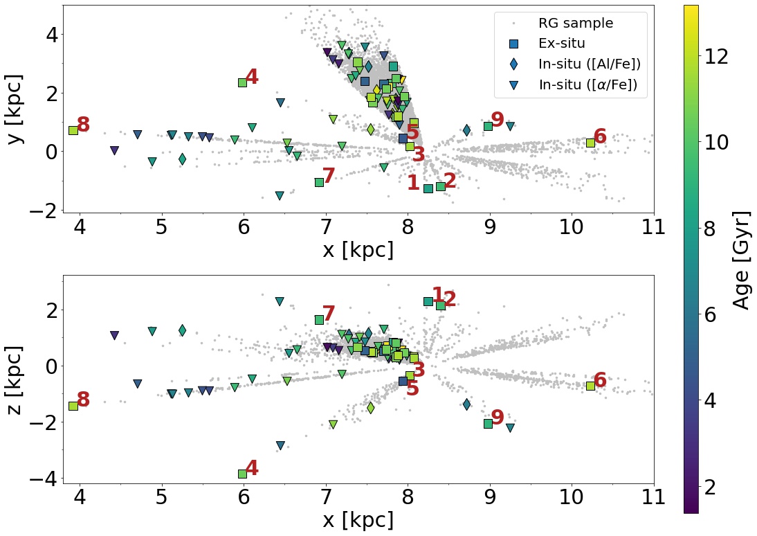
Figure 1: Position of the stellar sample in Galactocentric cartesian coordinates. Grey dots are the full red giant star sample while the coloured points mark the stars of interest in this work, coloured by their stellar age. The different symbols denote different selection criteria (for more information see Section 3) with the squares being the ex-situ stars. Indices are only added to the ex-situ from the K2 mission in the interest of clarity.

3 Selecting Ex-situ stars

Distinguishing ex-situ stars from in-situ stars is not a trivial process. The sample might be contaminated by in-situ stars that were for example heated by mergers and some ex-situ stars might have orbits that are not distinguishable from the in-situ stars. There is also a possibility of contamination of in-situ stars due to for example, ill-determined observed properties, or underestimated uncertainties. To combat this and get as pure a sample of ex-situ stars as possible, we make a stringent selection. This robust selection is based on a cut in dynamical space and two cuts in different chemical spaces (see Table 1). As mentioned in Section 1, the Milky Way has merged with several galaxies in the past, meaning it is possible that the ex-situ stars we find are not all from the same merger remnant (see Section 5.2). We therefore distinguish between ex-situ and GES stars throughout this work.

The first selection criterion is in dynamic space meaning in energy ($E$) and angular momentum ($L_{z}$). This has become a common method of identifying ex-situ and GES stars and was partly also how the GES stars were discovered in Helmi et al. (2018). We select stars with small and negative angular momentum ($L_{z}$ $<0.65$e$3$ kpc km s^-1). Negative angular momentum means that the stars are counter-rotating compared to the rest of the Milky Way stars, that have positive angular momenta and thus it is an indication that these stars are not formed in-situ. In Figure 2, the full red giant star sample is in gray and the stars from this dynamic selection are marked by coloured symbols. The full sample of Gaia eDR 3 stars (with RUWE$<1.4$) are shown in orange shade for easier comparison to other works. The selection leaves us with $78$ stars and we determine the ages for all of them.

The dynamics cut is not sufficient to fully exclude the in-situ stars. Therefore, we make two additional cuts in chemical space (see Table 1). The first is in [$\alpha$/Fe] vs [Fe/H] space as shown in Figure 3. Here, [$\alpha$/Fe] is defined as $\frac{1}{2}$([Mg/Fe]+[Si/Fe]) following Salaris et al. (2018). In this plot, there are two distinct populations, one that correlates with the in-situ stars at high [Fe/H] abundance and one at lower [Fe/H], which matches with our expectations of them being ex-situ stars. We make a division between these two populations with line at [$\alpha$/Fe]$>-0.55$[Fe/H]$-0.25$ (red line in Figure 3). All stars from the dynamical selection that fall above this criteria are marked with triangles and are denoted as in-situ stars. With this cut we sort out $48$ of the $78$ stars and classify them as in-situ stars.

Lastly a cut is made in [Mg/Mn] vs [Al/Fe] space based on the chemical evolution of galaxies described in Section 1. The lines dividing the populations are based on Horta et al. (2021) (see Figure 4 and Table 1). Here, stars in the upper left corner are regarded as ex-situ stars. Stars that are removed from the ex-situ sample due to this cut are marked with diamonds unless they were already removed due to the [$\alpha$/Fe] selection, in which case they remain denoted with triangles. This last cut removes $7$ additional stars and deem them in-situ stars.

Table 1: Selection criteria for ex-situ star classification

	This work	M21
1.	$L_{z}$ $<0.65\times 10^{3}$ kpc km s-1	e$\,>0.7$
2.	[$\alpha$/Fe]$\,<-\,0.55\,$[Fe/H]$\,-\,0.25$	[Mg/Fe]$\,<-0.2\,$[Fe/H]$\,+\,0.05$
3.	[Mg/Mn]$\,>1.8\,$[Al/Fe]$\,+\,0.35$
	[Mg/Mn]$\,>0.25$

In the end, only stars that are in the ex-situ sample in all three parameter spaces are classified as ex-situ stars and denoted with squares in all figures. We find a total of $23$ likely ex-situ stars in our sample. These stars are marked with indices in all figures for easier identification. The relation between indices and KIC and EPIC ID’s can be seen in LABEL:tab:All_stars. We note that of the $78$ stars purely selected in dynamical space only ${\sim}1/3$ are classified as ex-situ stars. This shows that a simple selection in $L_{z}$ can result in significant amounts of contamination.

In Figure 5, we show the stars in a number of different chemical spaces. Common for all is that the stars we select as ex-situ appear to be a different population than the gray points we expect to be in-situ stars. This strengthens our assumption that these stars indeed are formed in different galaxies.

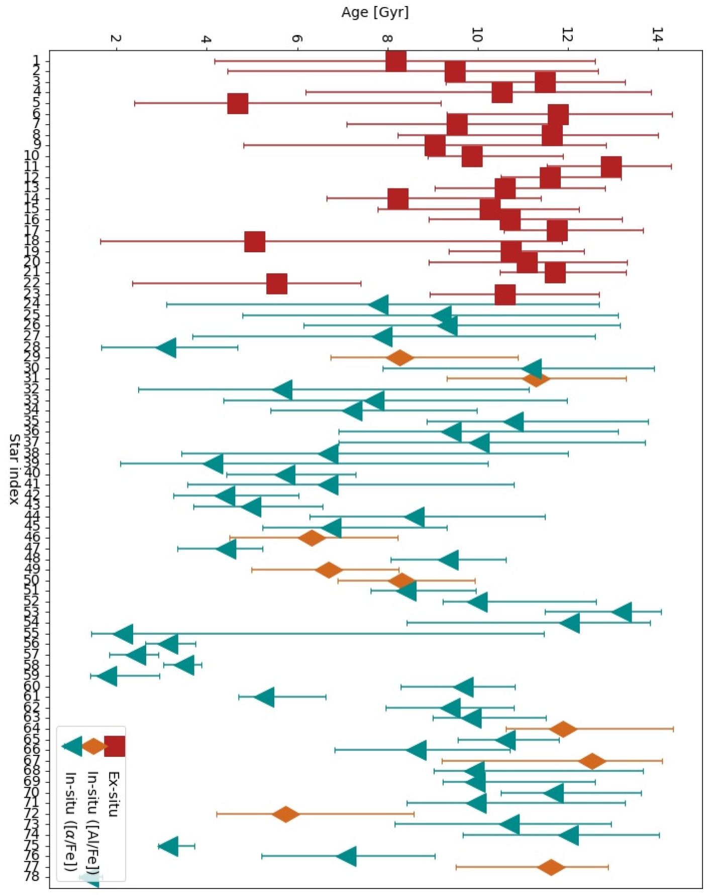
Figure 10: Ages of the stars with uncertainties. Indices match the ones used in other figures. Symbols are explained in Section 3.

Five of the classified in-situ stars are on retrograde orbits ($L_{z}$ $<0$ kpc km s^-1 in Figure 2) which is peculiar for in-situ stars. They are removed from the ex-situ sample based on chemistry but a follow-up spectroscopic survey of these stars could clarify their classifications. In this work, we keep them as in-situ and note it is stars #51, 53, 64, 67, and 77 in Figure 10 and LABEL:tab:All_stars.

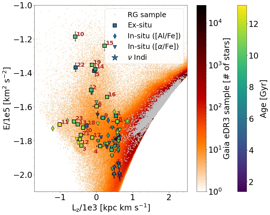
Figure 2: Distribution of stars in $L_{z}$-$E$ space. The gray points denote the full sample of RG stars, the different symbols denote the classification of our selected stars as described in Section 3, and the orange background stars are the full Gaia eDR3 sample. The star symbol is $\nu$ Indi with age from Chaplin et al. (2020). All ex-situ stars are marked with the indices corresponding to those in LABEL:tab:All_stars.

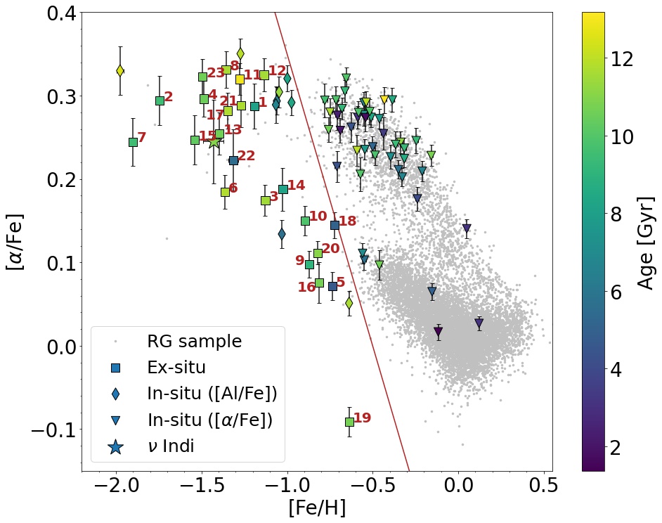
Figure 3: [$\alpha$/Fe] vs metallicity abundance. Markers, colours and indices are the same as in Figure 2. The red line marks our selection criterion (see Table 1). The metallicity for $\nu$ Indi is from Chaplin et al. (2020).

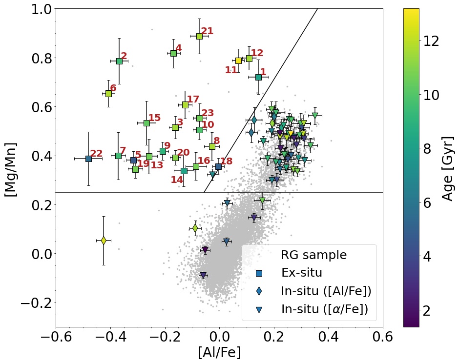
Figure 4: [Mg/Mn] vs [Al/Fe] abundance with lines from Horta et al. (2021) (see also Table 1). Markers, colours and indices are the same as in Figure 2.

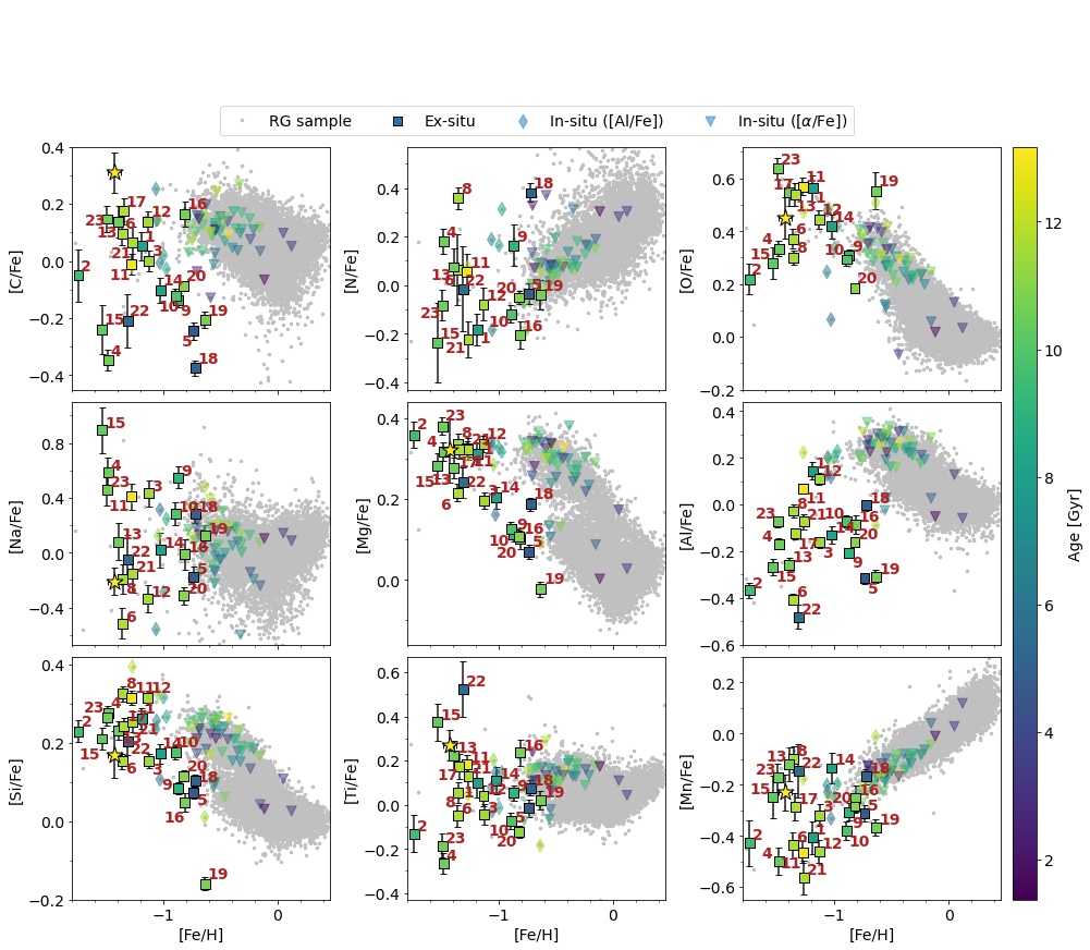
Figure 5: Different metallicities for our sample of red giant stars. Not all abundances were available for all stars. The colour and indices are the same as previous figures. All figures has [Fe/H] in the x-axis with the same scale.

4 Age Determination

In this section we describe the theory behind asteroseismology (Section 4.1) and how it is used for age determination. In Section 4.2 and Section 4.3 we present the code and grid used for the fitting and in Section 4.4 we describe the details of the stars that are fitted.

4.1 Asteroseismology

As mentioned in Section 1, we use constraints from asteroseismology to determine the stellar ages of our sample. Asteroseismology is the study of how the stars oscillate and vibrate. The great advantage of asteroseismology is that the pattern in the power spectrum of the photometric time series is structurally identical for all solar-like stars. The power spectrum pattern consists of frequencies ($\nu$) that have a very regular comb structure (at least for slowly rotating stars) and follow a Gaussian-like shape in power as a function of frequency (see e.g. Aerts et al., 2010; Basu, 2016). As solar-like oscillators shows this general structure, we can decompose this pattern into two global asteroseismic parameters: the large frequency separation ($\Delta\nu$) and the frequency at maximum power ($\nu_{\mathrm{max}}$). As the name suggests $\nu_{\mathrm{max}}$ is the frequency where the Gaussian-like distribution peaks and the large frequency separation ($\Delta\nu$) is the difference in frequency between oscillations of the same angular degrees ($l$) but of consecutive radial order ($n$) hence

$$\Delta\nu_{l}(n)=\nu_{n,l}-\nu_{n-1,l}.$$ (1)

Ulrich (1986) and Christensen-Dalsgaard (1988) have analytically shown that $\Delta\nu$ scales with radius ($R$) and mass ($M$) of the star in the following manner:

$$\frac{\Delta\nu}{\Delta\nu_{\odot}}\simeq\left(\frac{M}{\mathrm{M}_{\odot}}\right)^{1/2}\left(\frac{R}{\mathrm{R}_{\odot}}\right)^{-3/2}.$$ (2)

Furthermore, Brown et al. (1991), Kjeldsen & Bedding (1995) and Bedding & Kjeldsen (2003) found a semi-empirical scaling relation based on the frequency of maximum power, which scale with mass, radius, and effective surface temperature ($T_{\mathrm{eff}}$) of the star

$$\frac{\nu_{\mathrm{max}}}{\nu_{\mathrm{max},\odot}}\simeq\left(\frac{M}{\mathrm{M}_{\odot}}\right)\left(\frac{R}{\mathrm{R}_{\odot}}\right)^{-2}\left(\frac{{T}_{\mathrm{eff}}}{\mathrm{T}_{\mathrm{eff},\odot}}\right)^{-1/2}.$$ (3)

Combining Equation 2 and Equation 3, we can estimate the mass and radius of the star only based on the asteroseismic parameters and the surface temperature. The mass and radius are determined as

$$\left(\frac{M}{\mathrm{M}_{\odot}}\right)\simeq\left(\frac{\nu_{\mathrm{max}}}{\nu_{\mathrm{max},\odot}}\right)^{3}\left(\frac{\Delta\nu}{\Delta\nu_{\odot}}\right)^{-4}\left(\frac{T_{\mathrm{eff}}}{\mathrm{T}_{\mathrm{eff},\odot}}\right)^{3/2}$$ (4)

and

$$\left(\frac{R}{\mathrm{R}_{\odot}}\right)\simeq\left(\frac{\nu_{\mathrm{max}}}{\nu_{\mathrm{max},\odot}}\right)\left(\frac{\Delta\nu}{\Delta\nu_{\odot}}\right)^{-2}\left(\frac{T_{\mathrm{eff}}}{\mathrm{T}_{\mathrm{eff},\odot}}\right)^{1/2}.$$ (5)

This way the asteroseismic parameters are directly related to the physical properties of the star. The scaling relations between the observables $\Delta\nu$ and $\nu_{\mathrm{max}}$ (along with $T_{\mathrm{eff}}$) and the stellar properties like the mass and radius of the star are one of the great successes of asteroseismology. Asteroseismology narrows down the likely parameter space and provides tight constraints valuable for age determination.

The resolution of the power spectra depends on for example the length of time series data, and if the resolution is good enough individual mode frequencies can be extracted. This is especially the case for many Kepler stars. Individual frequencies can greatly improve the precision of the fits because they can constrain the stellar properties even further than $\Delta\nu$ and $\nu_{\mathrm{max}}$.

For extraction and identification of the frequencies we use the python package PBjam (Nielsen et al., 2021). The frequencies have been corrected for the Doppler shift caused by the stellar line-of-sight movement in accordance with Davies et al. (2014). If individual modes are not available we use the $\nu_{\mathrm{max}}$ and $\Delta\nu$ values from the syd pipeline (Huber et al., 2009) and an AI-detector for the classification of the evolutionary state (Yu et al., 2018; Hon et al., 2018; Zinn et al., 2020). For many of the K2 stars an AI-vetter was used to determine the quality of the $\Delta\nu$ measurements (Reyes et al. 2021, submitted). This algorithm provides a metric for the relation of the purity and completeness and we only accept stars with this number larger than 0.6, which corresponds to a purity of ${\sim}97$% and a completeness of ${\sim}93$%. To account for systematic uncertainties of the K2 stars, we added a percentage of $\Delta\nu$ and $\nu_{\mathrm{max}}$ to the uncertainties based on the standard deviation of the correction factors of different pipelines in Zinn et al. (2021, their Table 3). We estimated the systematic $\nu_{\mathrm{max}}$ uncertainty to be $0.3\%$ for stars that are known to be in the red giant branch (RGB) phase and $0.7\%$ for those in the red clump (RC) (or unknown) phase. The systematic $\Delta\nu$ uncertainty is estimated to be $0.3\%$ for RGB and $0.4\%$ for RC (or unknown) phase.

For the stars that only had $\Delta\nu$ and $\nu_{\mathrm{max}}$ we made a consistency check with the APOKASC sample (Pinsonneault et al., 2018) and the K2 GAP DR3 sample (Zinn et al., 2021) for the Kepler and K2 stars, respectively. All stars in this work that were available in one of the two studies had consistent $\Delta\nu$ and $\nu_{\mathrm{max}}$ values within $\pm 1\sigma$ of the respective studies, except star #6. It appears the syd pipeline overestimates the $\nu_{\mathrm{max}}$ of this star with ${\sim}2\mu$Hz compared to other pipelines. Computing the stellar properties for star #6 with the K2 GAP DR3 $\nu_{\mathrm{max}}$ also resulted in a more consistent fit with respect to the other input parameters and we chose to use this value of $\nu_{\mathrm{max}}$ for this star. For all other stars we keep the values from the syd pipeline.

4.2 basta

To determine the stellar parameters we use the BAyesian STellar Algorithm (basta; Silva Aguirre et al., 2015, 2017; Aguirre Børsen-Koch et al., 2021). The algorithm uses a pre-calculated grid of stellar tracks and Bayesian statistics to find the best fitting stellar parameters for each star. basta allows for prior probability distributions to be taking into account when calculating the fits. We use the Salpeter initial mass function (Salpeter, 1955) to account for the expected mass distribution of stars, favouring low-mass stars as the most abundant. We use the two-term surface correction described in Ball & Gizon (2014). Additionally, we include an upper limit on the stellar ages of 15 Gyr. This is done to avoid nonphysical solutions for stars older than the age of the universe. Despite the solutions not being physical at above the age of the universe (13.7 Gyr), they can still hold statistical significance and we do therefore not truncate the solutions at 13.7 Gyr but allow them to stretch to 15 Gyr. For the remaining parameters we use uniform priors.

4.3 The grid

As mentioned above, basta uses a grid of stellar models to fit the stars. We build a quasi-random sampled (sobol; Sobol, 1967) grid with ${\sim}8000$ evolutionary tracks of stellar models using the Garching Stellar Evolution Code (Weiss & Schlattl, 2008, Garstec). The mass range of the grid is between $0.7$ and $2.0$ M_⊙, the initial metallicity [Fe/H]_ini varies between $-2.4$ and $0.1$ dex, the $\alpha$-enhancement ranged from $-0.2$ to $0.6$ dex in steps of $0.1$ dex. The mass loss ($\eta$) ranges from $0.0$ to $0.3$ following the Reimers (1977) formalism. Convection in the models are parameterised using mixing-length theory (Böhm-Vitense, 1958) and the mixing-length parameter is kept constant at the solar-calibrated value of $1.789$ as determined from a standard solar model calibration to the Asplund et al. (2009) abundances. The initial helium is assumed to be 0.248 (Fields et al., 2020) and the helium-to-metal ratio is $\Delta Y/\Delta Z=1.4$. The stellar models are evolved from pre-main sequence to the beginning of the RGB whereafter the models are saved and frequencies computed along the RGB, through the RC and all the way to the asymptotic giant branch (AGB). This provides us with a very fine grid of stellar models in the RGB and RC phase. For all models the radial oscillation modes ($l=0$) are computed using the Aarhus adiabatic oscillation package (adipls; Christensen-Dalsgaard, 2008).

4.4 Fits

To determine the ages of the stars we use the observed parameters [$\alpha$/Fe], [Fe/H], $T_{\mathrm{eff}}$, asteroseismic values (individual frequencies or $\Delta\nu$ and $\nu_{\mathrm{max}}$, as well as evolutionary phase when available) and distance. We use the parallax and three photometric filters when fitting the distances to the stars (2MASS filters $J$, $H$, and $K_{s}$) as well as the dust map from Green et al. (2019) for computing the extinction. These parameters are mapped to our grid of stellar models to find the best match.

When we fit the stars, different constraints can point towards slightly different solutions. Especially the constraint of the parallax and the photometric colours can be in tension with the asteroseismic solutions. This is typically due to inaccurate or incorrect determination of one or more of the parameters, underestimates of the uncertainties, or models inaccuracies. As a test of robustness, we fitted the stars in three different ways: (i) by fitting all the parameters mentioned above, (ii) by fitting everything excluding the distance (parallax and photometric filters), and (iii) fitting everything excluding the asteroseismic values. Since the asteroseismic values and distance both give a direct measure of the radius of the stars (see Equation 5), we compare the solution for the radius of the three fitting methods. In the cases where the calculated median radius of the fit with all parameters (i) agrees within $\pm 1\sigma$ with the solution of both other fits (ii and iii), we accept the solution (i) as robust and it is chosen because adding additional information improves the uncertainties of the solution. This check is in addition to a manual inspection of the probability distributions, to insure the solution for example does not interfere with the edge of the grid.

For some stars, the three fits did not match up and gave two or even three very different solutions. The fit with all the parameters (i) would then artificially be located between the two solutions of (ii) and (iii) or pushed to the edge of the two. In these cases, we will chose to trust case (ii), that is the fits including asteroseismic constraints but excluding the constraints from photometry and astrometry. We choose the asteroseismic solution as many aspects can influence the distance fit such as poorly determined parallax, colours or dust map to name some. Choosing the asteroseismic solution over the full fit mainly affects the uncertainties of the solution. Because our selection of the stars is based on $E$ and $L_{z}$ (which is calculated with the parallax) we check that the selection is not affected if we now adopted the distance output form basta in the selection (by recalculating E and Lz). While some of the stars did move slightly in $E$ and $L_{z}$ space, they where all still part of our selection. In LABEL:tab:All_stars, we note which stars have been fitted with what method and whether we used individual frequencies or $\Delta\nu$ and $\nu_{\mathrm{max}}$. Ten of the $23$ ex-situ stars and $19$ of the $55$ in-situ stars have been fitted without the distance.

The determined ages of the stars are shown as colour coding in Figure 1, 2, 3, 4, and 5, the ages of the ex-situ stars with uncertainties are shown in Figure 6 and for all $78$ stars in Figure 10 and LABEL:tab:All_stars.

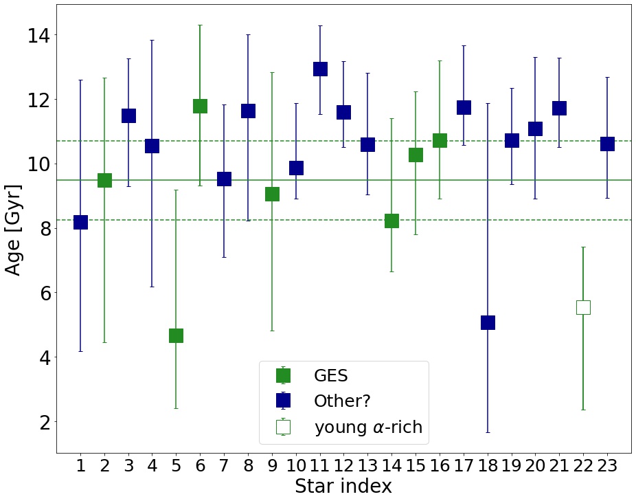
Figure 6: Ages of the ex-situ stars with uncertainties. Indices match the ones used in other figures. Green symbols are the ones we classify as GES stars and blue stars are the ones that might originate from other mergers. The hollow symbol for star #22 marks that this might be a young $\alpha$-rich star. The full horizontal line indicates the mean age of the green points (the GES stars) and the dashed lines indicate the standard deviation.

5 Results and Discussion

In this section we present the results of the age determinations. In Section 5.1, we discuss some stars with peculiar solutions and how we treat them. In Section 5.2 we discuss the origin of the ex-situ stars and how the ages can give us an estimate of the upper limits of the merger times.

5.1 Peculiar stars

A peculiar case among the ex-situ stars is star #22, which is very young compared to the rest of the ex-situ stars (see Figure 6 or LABEL:tab:All_stars). Although it is likely a GES star (see Section 5.2.1) it appears too young because GES does not have any recent star formation. This is the Kepler star KIC 8694070, which has individual mode frequencies available. The solutions from the fits with all parameters and those without distance did not agree for this star (see discussion in Section 4.4), and we defaulted to using the fit without the distance in this case. The asteroseismic fit is good and we trust the solution, which could mean this is a young $\alpha$-rich star. As described above, the asteroseismic parameters are used to find a mass and a radius of the stars, which can then be compared to an age with stellar evolutionary tracks to find the best correlation. If the star was part of a multistellar system where mass transfer have occurred, the current mass could exceed the initial mass of the star and make the star appear younger than its actual age. This is normally known as blue stragglers or in the case of old red giant stars as young $\alpha$-rich stars (Martig et al., 2015; Zhang et al., 2021). This means that this star is likely not actually this young and we exclude it from any determination of mean ages in later calculations.

Star #4 has a $\Delta\nu$ $=0.64\pm 0.12\mu$Hz and our grid is limited to $\Delta\nu$ $>0.6\mu$Hz, which means this star is very close to the edge of the grid. This star is also a K2 stars with a short timeseries and a very small $\nu_{\mathrm{max}}$ $=4.79\pm 0.62\mu$Hz. Asteroseismic values this low can be very hard to measure for stars with short timeseries and we have therefore chosen to not fit $\Delta\nu$ and $\nu_{\mathrm{max}}$ for this star, as we do not find them reliable. With more data from for example the TESS satellite (Ricker et al., 2015) it is possible that the asteroseismology could be improved and used for fitting in the future.

5.2 Ex-situ

Through our selection criteria we have determined which stars are ex-situ stars in our sample. Associating them with a specific merged galaxy is more tricky. There are several studies denoting stars and globular clusters to galaxy remnants such as Massari et al. (2019); Koppelman et al. (2019); Kruijssen et al. (2020); Naidu et al. (2021). The issue with comparison between different works are for example that they use different potentials to calculate the dynamics, making it hard to do direct comparison. The classification within the same potential is also not always clear and remnant stars from different galaxies overlap in both kinematic and chemical space making it nearly impossible to distinguish. In Figure 7, we show the ex-situ stars similar to Figure 2 but colour coded according to eccentricity ($e$). It is generally accepted that GES stars have larger $E$ than stars with similar $L_{z}$ and large $e$ but the exact boundaries are not clear. The difference in chemistry (see Figure 8) between our ex-situ stars suggests that these are not all of the same origin. It is possible that all these are indeed GES stars but due to the large spread in dynamics and chemistry we have chosen to make a very conservative classification of the GES stars which is described in Section 5.2.1. In Section 5.2.2 and Section 5.2.3, we discuss other possible origins of the remaining stars.

As mentioned in Section 1, the accreted galaxies are disrupted during the merger, which quenches star formation. The mean age of the stars originating in a galaxy can, therefore, be interpreted as an upper limit for when the galaxy was disrupted during the merger. We present such mean values below. The mean age is calculated with a bootstrap method with $1000$ iterations.

In general, all the stars are older than $8$ Gyr (except for star #22), which is in good agreement with expected ages for accreted stars (see e.g. Kruijssen et al., 2020).

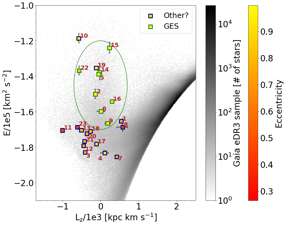
Figure 7: Similar to Figure 2 but with only ex-situ stars colour coded according to eccentricity of the orbits. In gray is the full sample of Gaia eDR3 stars. The green outline denotes stars that we classify as GES and the blue as possibly originating from other merger galaxies. The green circle shows how we select the stars that are classifies as GES.

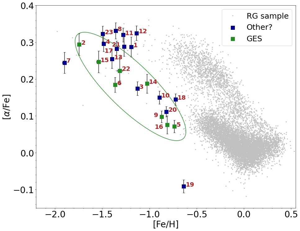
Figure 8: Similar to Figure 3 but only ex-situ stars coloured according to our classification as GES (green) or possibly originating from other mergers (blue)

5.2.1 GES

As mentioned, there is not yet a widely accepted way of determining exactly where the ex-situ stars originate from. Our sample of ex-situ stars can be compared directly to the sample of GES stars in Massari et al. (2019) (see their Figure 2) as they use the same potential as we do. All our stars are within the same region in $E$ vs $L_{z}$ space as their GES stars although some are very close to the edges. Naidu et al. (2021) and M21 classify GES stars as those with $e>0.7$. This is the case for all of our ex-situ stars apart from #8, 11 and 23. However in Figure 8, we expect stars from the same galaxies to follow a similar trend but there is an almost $0.2$ dex difference in [$\alpha$/Fe] between stars of the same [Fe/H] (stars #3, 14 and #1, 12). This could mean that the stars are not of the same origin. To be conservative we classify stars as GES only if they have a high $E$ and just around $L_{z}$ $=0$ as well as a similar trend in metallicity. These stars are marked by a green circle in Figure 7 and Figure 8. The stars that are classified as GES are green (have a green edge) in these two figures and stars that are not in both classifications are blue. This is also the colour coding in Figure 6. We note that star #22 is part of this selection but as discussed in Section 5.1 the age of this star is likely inaccurate and it is excluded from the mean age calculation. The mean age of our selected GES stars is $9.5_{-1.3}^{+1.2}$ Gyr.

This might be a too conservative classification of GES stars. Especially the lower $E$ boundary in Figure 7 could be excluding stars that appear to be GES stars in for example Figure 8. However, the lower $E$ region is also where in-situ stars are potential contaminants and reducing the $E$ boundary could lead too a less pure GES sample. We therefore chose to be conservative in our selection and only include stars at high $E$. As more studies on the merger galaxies are made it is possible that more stars from our sample turns out to be GES stars. We present the ages of individual stars making it easy for later works to use the ages of the stars should improved selection criteria be determined. For reference, we note that the mean age of the full sample (excluding #22) is $10.1\pm 0.7$ Gyr and the mean age of the stars with $e>0.7$ is $9.8\pm 0.8$ Gyr.

Comparison with M21

M21 did a similar study to ours but used only RGB Kepler stars, different selections (see Table 1), and a different code to calculate the ages. They further used Gaia DR2 (Gaia Collaboration et al., 2018) and APOGEE DR14 (Majewski et al., 2017) where we use eDR3 and DR16, respectively. In our ex-situ sample we find the same stars as they do except for KIC 8869235 because this was pruned in our selection due to a bad flag in STAR$\_$WARN. The comparison between our ages and the ages presented by M21 is shown in Figure 9. The ages agree well between the two studies and differences can be attributed to slightly different metallicities, and different software and models. Although we get similar ages for the stars we do not classify the same stars as GES but we do classify them as ex-situ. From the sample selected by M21 we do not classify star #10, 17 and 19 as GES. On the other hand, as mentioned above, if we were to use the criteria proposed by M21 all stars except #8, 11 and 23 would be GES stars. While our selection might be too conservative it is possible that the one presented in M21 is too broad. M21 calculated a mean age of the GES stars of $9.7\pm 0.6$ Gyr and we get $9.5_{-1.3}^{+1.2}$ Gyr for our selection of GES stars. The age of our stars with $e>0.7$ is $9.8\pm 0.8$ Gyr. All these ages are in agreement further enhancing the conclusion that the merger time is less than ${\sim}10$ Gyr ago.

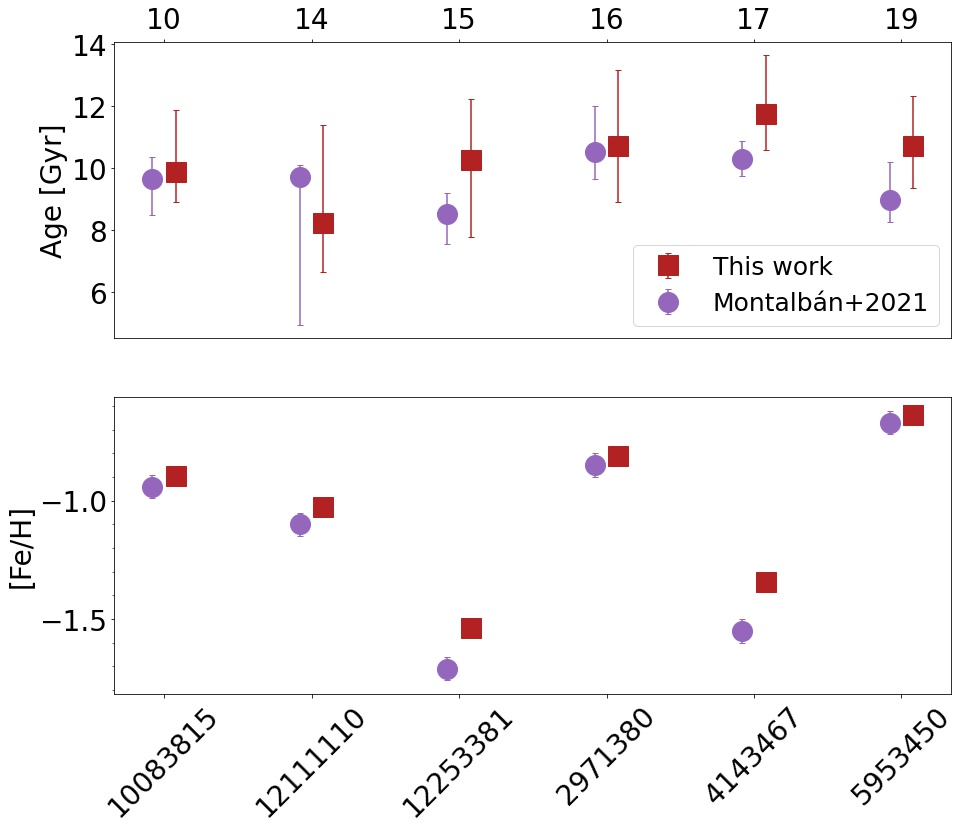
Figure 9: Comparison between our results and those of the same stars from M21. Top: ages. Bottom: iron abundance. While M21 uses APOGEE DR14, we use DR16. All stars are Kepler stars with KIC ID’s on x-axis of bottom panel and indexes matching our figures on top for cross identification with the other figures presented in this work.

5.2.2 Kraken

Another galaxy some of the stars could belong to is Kraken (Kruijssen et al., 2019; Massari et al., 2019; Kruijssen et al., 2020). Kraken is expected to have had similar mass as GES (${\sim}3\cdot 10^{8}$M_⊙) and to have merged with the nascent Milky Way before GES. These stars are located at low $E$ and at $\lesssim 7$ kpc from the galactic centre. Star #8 is the closest star in our sample to the Galactic centre at ${\sim}4$ kpc. It is, however, at higher $E$ than we expect the Kraken stars to be based on the globular clusters from Massari et al. (2019). It might, therefore, originate from somewhere else. Stars #3, 4, 7, and possibly 12 are closer to the expected $E$ for Kraken and stars #4 and 7 are furthermore closer than ${\sim}7$ kpc to the Galactic centre. It is currently not clear where the boundaries of the Kraken remnants are and we can therefore not classify any of our stars as such with certainty. The accretion time of the Kraken was estimated to be $10.9^{+0.4}_{-0.7}$ Gyr by Kruijssen et al. (2020) which agrees well with all these stars being old according to our calculations. Until we have more stars in this region or a tighter constraint on their properties compared to other ex-situ stars, it is unknown if and how many Kraken stars there are in our sample. If we assume stars #3, 4, 7, and 12 are Kraken stars the mean age is $9.2_{-1.7}^{+1.9}$ Gyr, which is well within the estimate made by Kruijssen et al. (2020).

5.2.3 Other possible origins

The stars that are not GES stars (or Kraken stars) could have different origins. There are some that are close to our selection criteria boundaries in both [$\alpha$/Fe] and [Al/Fe] (see stars #1, 11, 12, and 18 in Figure 3 and Figure 4), which could make them in-situ stars. It is also possible that they belong to Thamnos (Koppelman et al., 2019) or Sequoia (Myeong et al., 2019) or some other yet undefined merger event. However, there is no clear characterization yet that would allow us to do a firm statistically based membership probability or association and it is not possible to confidently classify their origin. As more observations comes in from surveys such as Gaia and APOGEE it might be possible to classify them in the future. With more stars becoming available with TESS and other asteroseismic surveys we will also be able to get ages for more of these ex-situ stars, which might make it possible to make classifications based on the ages of the stars in the future. For now we present the ages of the stars and leave further classification for future works.

6 Conclusion

In this paper, we examine a sample of nearly $12,000$ Kepler and K2 stars and we find $23$ stars of ex-situ origin. Our selection is based on angular momentum ($L_{z}$), energy ($E$), and the [$\alpha$/Fe], [Fe/H], [Al/Fe], and [Mg/Mn] abundances making it very stringent to insure a high likelihood of choosing only ex-situ stars.

Using asteroseismology from Kepler and K2, 6D phase space data from Gaia eDR3, along with temperature and metallicity from APOGEE DR16, we derive their stellar properties using the Bayesian framework of basta. We present ages for all $23$ ex-situ stars as well as $55$ in-situ stars.

All the ex-situ stars are consistent with being older than $8$ Gyr (except for one that is likely a young $\alpha$-rich star), which is expected because most massive mergers took place more than $8$ Gyr ago.

We make a conservative classification of the ex-situ stars and denote eight of them to be GES stars with a mean age of $9.5_{-1.3}^{+1.2}$ Gyr, which agrees with current estimates of a merger time around $8-10$ Gyr ago. We compare our stellar ages to those found be Montalbán et al. (2021) and demonstrate similar results but based on different methods. The classification of GES stars between the studies deviate but we get similar mean ages of the GES stars regardless.

The remaining $15$ stars are ex-situ stars of debatable origin and some of them could also belong to GES. It is possible that four of these stars belong to the dwarf galaxy Kraken and their mean ages are estimated to be $9.2_{-1.7}^{+1.9}$ Gyr in agreement with estimates from Kruijssen et al. (2020).

With more data becoming available from for example the TESS mission, it might be possible to find even more asteroseismic merger remnant stars in the future. With more stars with precise ages it might be possible to distinguish stars from different origins based on not only their kinematics and chemistry but also their ages.

Due to the large impact mergers have had on the Milky Way’s evolution, the stars presented in this work contribute important information to better understand how the mergers happened and what impacted they have had on our present day Milky Way.

Software

The research for this publication was coded in python (v. 3.8.5; Van Rossum & Drake, 2009) and included its packages astropy (v. 4.0.2; Astropy Collaboration et al., 2013, 2018), galpy (v. 1.6.0; Bovy, 2015) matplotlib (v. 3.3.2; Hunter, 2007), numpy (v. 1.19.2; Harris et al., 2020), vaex (v. 3.0.0; Breddels & Veljanoski, 2018), IPython (v. 7.19.0; Pérez & Granger, 2007), Jupyter (v. 2.2.6; Kluyver et al., 2016) and Spyder (v. 4.1.5; Raybaut, 2009). For frequency peak bagging we used PBjam (Nielsen et al., 2021) and for stellar properties determination we used basta (Aguirre Børsen-Koch et al., 2021).

Data Availability

The data underlying this article will be available in the article and in its online supplementary material upon publication.

Appendix A Stars in our sample

Table 2: Table of stars from our sample. The columns contain the index of the stars used throughout the paper (INDEX), the ID of the stars where "Kepler" denotes stars with KIC ID’s and K2Cx denotes stars from the K2 mission with x corresponding to the campaign number and corresponding EPIC ID. The asteroseismic parameters from PBJam or the SYD pipeline in $\mu$Hz. The following column is the distance to the Galactic centre in kpc and the eccentricity of the stars. The distance, radius and ages with uncertainties (16th and 84th percentile from the posterior distribution) are derived from basta in kpc, R_⊙ and Gyr, respectively. The second to last column contain information about how each star was fitted. "Indi" denotes stars that had individual frequencies available, "Seis" indicates stars that only had $\nu_{\mathrm{max}}$ and $\Delta\nu$ available and "(no) dist" denotes stars where the distance was (not) fitted. The last column contains our classification of the star.

INDEX	ID	$\Delta\nu$	$\nu_{\mathrm{max}}$	R${}_{\text{GC}}$	e	Distance	R∗	Age	FIT	Classification
1	K2C1 201609020	$3.99\pm 0.02$	$31.63\pm 0.91$	$8.35\pm 0.01$	$0.78\pm 0.02$	$2910_{-64}^{+91}$	$10.1_{-0.4}^{+0.7}$	$8.19_{-4.02}^{+4.41}$	Indi, no dist	Ex-situ
2	K2C1 201709805	$3.68\pm 0.03$	$30.06\pm 0.86$	$8.49\pm 0.01$	$0.97\pm 0.01$	$3126_{-54}^{+68}$	$10.4_{-0.3}^{+0.8}$	$9.49_{-5.03}^{+3.17}$	Indi, no dist	GES
3	K2C3 205934106	$13.24\pm 0.04$	$145.94\pm 4.28$	$8.02\pm 0.01$	$0.77\pm 0.01$	$465_{-7}^{+7}$	$4.4_{-0.1}^{+0.1}$	$11.48_{-2.19}^{+1.78}$	Indi, dist	Ex-situ
4	K2C3 206077646	$0.64\pm 0.12$	$4.79\pm 0.62$	$6.42\pm 0.15$	$0.92\pm 0.07$	$5134_{-172}^{+183}$	$19.5_{-1.4}^{+1.6}$	$10.54_{-4.35}^{+5.49}$	No seis, dist	Ex-situ
5	K2C3 206516677	$3.96\pm 0.06$	$30.19\pm 2.05$	$7.95\pm 0.01$	$0.99\pm 0.01$	$957_{-40}^{+42}$	$11.0_{-0.8}^{+0.9}$	$4.67_{-2.27}^{+4.50}$	Seis, no dist	GES
6	K2C4 211001845	$3.49\pm 0.08$	$27.59\pm 0.98$	$10.23\pm 0.08$	$0.98\pm 0.03$	$2289_{-38}^{+44}$	$10.5_{-0.2}^{+0.3}$	$11.78_{-2.47}^{+4.06}$	Seis, no dist	GES
7	K2C6 212319585	$3.73\pm 0.02$	$27.00\pm 1.28$	$7.00\pm 0.05$	$0.72\pm 0.03$	$2302_{-30}^{+35}$	$10.3_{-0.2}^{+0.3}$	$9.53_{-2.43}^{+2.31}$	Indi, dist	Ex-situ
8	K2C7 213616808	$1.23\pm 0.05$	$6.32\pm 1.96$	$3.98\pm 0.62$	$0.44\pm 0.16$	$4810_{-93}^{+98}$	$21.7_{-0.7}^{+0.8}$	$11.65_{-3.41}^{+2.36}$	Seis, dist	Ex-situ
9	K2C8 220238966	$4.10\pm 0.03$	$30.78\pm 2.09$	$9.02\pm 0.04$	$0.93\pm 0.03$	$2686_{-53}^{+70}$	$9.7_{-0.3}^{+0.6}$	$9.05_{-4.23}^{+3.78}$	Indi, no dist	GES
10	Kepler 10083815	$2.59\pm 0.01$	$17.99\pm 0.38$	$8.14\pm 0.01$	$0.93\pm 0.01$	$2415_{-21}^{+20}$	$13.0_{-0.2}^{+0.2}$	$9.87_{-0.97}^{+2.00}$	Indi, dist	Ex-situ
11	Kepler 10460723	$3.14\pm 0.02$	$22.97\pm 0.45$	$8.07\pm 0.01$	$0.49\pm 0.01$	$2400_{-19}^{+16}$	$11.1_{-0.1}^{+0.1}$	$12.94_{-1.41}^{+1.34}$	Indi, dist	Ex-situ
12	Kepler 11563791	$5.04\pm 0.03$	$43.03\pm 0.51$	$8.13\pm 0.01$	$0.73\pm 0.01$	$978_{-7}^{+6}$	$8.2_{-0.1}^{+0.1}$	$11.60_{-1.09}^{+1.57}$	Indi, dist	Ex-situ
13	Kepler 11566038	$3.95\pm 0.03$	$31.36\pm 0.32$	$8.18\pm 0.01$	$0.79\pm 0.01$	$1945_{-20}^{+22}$	$9.7_{-0.2}^{+0.2}$	$10.60_{-1.56}^{+2.21}$	Indi, dist	Ex-situ
14	Kepler 12111110	$3.75\pm 0.02$	$29.57\pm 0.37$	$8.34\pm 0.03$	$0.99\pm 0.01$	$3052_{-70}^{+53}$	$10.5_{-0.4}^{+0.3}$	$8.22_{-1.57}^{+3.18}$	Indi, dist	GES
15	Kepler 12253381	$3.03\pm 0.02$	$22.00\pm 0.40$	$8.24\pm 0.01$	$0.97\pm 0.01$	$2795_{-42}^{+41}$	$11.6_{-0.2}^{+0.3}$	$10.27_{-2.48}^{+1.96}$	Indi, no dist	GES
16	Kepler 2971380	$7.88\pm 0.03$	$77.26\pm 0.70$	$7.75\pm 0.01$	$0.91\pm 0.01$	$1552_{-19}^{+25}$	$6.2_{-0.1}^{+0.1}$	$10.72_{-1.81}^{+2.46}$	Indi, no dist	GES
17	Kepler 4143467	$5.63\pm 0.02$	$48.96\pm 0.57$	$7.77\pm 0.01$	$0.93\pm 0.01$	$2009_{-18}^{+21}$	$7.6_{-0.1}^{+0.1}$	$11.75_{-1.17}^{+1.91}$	Indi, dist	Ex-situ
18	Kepler 5446927	$2.91\pm 0.03$	$21.88\pm 0.38$	$7.85\pm 0.01$	$0.88\pm 0.01$	$2184_{-107}^{+379}$	$13.2_{-1.3}^{+1.8}$	$5.06_{-3.41}^{+6.80}$	Indi, no dist	Ex-situ
19	Kepler 5953450	$12.69\pm 0.05$	$140.87\pm 0.83$	$7.94\pm 0.01$	$0.98\pm 0.01$	$1250_{-6}^{+9}$	$4.6_{-0.1}^{+0.1}$	$10.73_{-1.36}^{+1.62}$	Indi, dist	Ex-situ
20	Kepler 6865157	$1.57\pm 0.07$	$9.05\pm 0.28$	$7.99\pm 0.01$	$0.75\pm 0.01$	$3177_{-41}^{+46}$	$18.4_{-0.4}^{+0.5}$	$11.08_{-2.17}^{+2.21}$	Seis, dist	Ex-situ
21	Kepler 7948268	$11.45\pm 0.04$	$120.45\pm 0.82$	$7.97\pm 0.01$	$0.80\pm 0.01$	$1283_{-12}^{+10}$	$4.8_{-0.1}^{+0.1}$	$11.71_{-1.22}^{+1.57}$	Indi, dist	Ex-situ
22	Kepler 8694070	$4.63\pm 0.04$	$33.66\pm 0.42$	$8.04\pm 0.01$	$0.88\pm 0.01$	$2701_{-41}^{+41}$	$9.7_{-0.3}^{+1.1}$	$5.54_{-3.19}^{+1.88}$	Indi, no dist	GES
23	Kepler 9339711	$2.84\pm 0.01$	$20.51\pm 0.31$	$8.03\pm 0.01$	$0.45\pm 0.01$	$2266_{-26}^{+21}$	$12.1_{-0.2}^{+0.2}$	$10.61_{-1.68}^{+2.08}$	Indi, dist	Ex-situ
24	K2C11 204785972	$3.34\pm 0.17$	$23.10\pm 1.69$	$6.55\pm 0.04$	$0.68\pm 0.01$	$2000_{-59}^{+69}$	$12.0_{-0.8}^{+1.7}$	$7.79_{-4.69}^{+4.89}$	Seis, no dist	In-situ
25	K2C17 251512185	$4.73\pm 0.34$	$40.18\pm 0.77$	$7.73\pm 0.01$	$0.85\pm 0.03$	$1554_{-42}^{+51}$	$9.1_{-0.5}^{+0.8}$	$9.18_{-4.38}^{+3.92}$	Seis, no dist	In-situ
26	K2C2 204298932	$1.69\pm 0.05$	$10.30\pm 0.30$	$6.65\pm 0.04$	$0.97\pm 0.03$	$1782_{-69}^{+76}$	$18.3_{-0.7}^{+1.0}$	$9.31_{-3.16}^{+3.84}$	Seis, no dist	In-situ
27	K2C2 204466120	$1.68\pm 0.05$	$10.97\pm 1.59$	$4.90\pm 0.25$	$0.47\pm 0.03$	$4045_{-116}^{+135}$	$18.7_{-0.9}^{+1.4}$	$7.87_{-4.18}^{+4.73}$	Seis, no dist	In-situ
28	K2C2 204966489	$2.26\pm 0.11$	$18.45\pm 0.37$	$4.42\pm 0.24$	$0.27\pm 0.02$	$3212_{-100}^{+90}$	$16.7_{-1.0}^{+1.5}$	$3.08_{-1.42}^{+1.59}$	Seis, no dist	In-situ
29	K2C2 205083494	$1.21\pm 0.03$	$6.80\pm 0.20$	$5.26\pm 0.14$	$0.40\pm 0.02$	$3225_{-53}^{+51}$	$22.3_{-0.6}^{+0.6}$	$8.27_{-1.52}^{+2.61}$	Seis, dist	In-situ
30	K2C3 205972576	$4.08\pm 0.12$	$28.51\pm 6.21$	$7.17\pm 0.05$	$0.82\pm 0.03$	$2697_{-43}^{+49}$	$10.2_{-0.4}^{+0.3}$	$11.18_{-3.29}^{+2.71}$	Seis, dist	In-situ
31	K2C3 205997746	$5.69\pm 0.03$	$51.06\pm 0.86$	$7.59\pm 0.02$	$0.73\pm 0.02$	$1859_{-21}^{+22}$	$7.6_{-0.1}^{+0.2}$	$11.29_{-1.98}^{+1.98}$	Indi, dist	In-situ
32	K2C3 206011766	$1.22\pm 0.09$	$7.34\pm 0.20$	$6.66\pm 0.09$	$0.63\pm 0.04$	$4145_{-168}^{+351}$	$23.2_{-2.1}^{+3.0}$	$5.66_{-3.17}^{+5.47}$	Seis, no dist	In-situ
33	K2C6 212297999	$2.60\pm 0.07$	$19.31\pm 0.34$	$7.00\pm 0.04$	$0.74\pm 0.02$	$2485_{-73}^{+80}$	$13.8_{-0.7}^{+1.0}$	$7.69_{-3.32}^{+4.28}$	Seis, no dist	In-situ
34	K2C6 212302713	$3.94\pm 0.02$	$31.94\pm 0.79$	$6.62\pm 0.08$	$0.56\pm 0.04$	$3175_{-48}^{+46}$	$10.6_{-0.3}^{+0.3}$	$7.21_{-1.80}^{+2.76}$	Indi, dist	In-situ
35	K2C7 213463719	$5.80\pm 0.02$	$54.92\pm 1.38$	$6.54\pm 0.07$	$0.69\pm 0.03$	$1825_{-21}^{+23}$	$7.9_{-0.2}^{+0.2}$	$10.78_{-1.92}^{+2.98}$	Indi, dist	In-situ
36	K2C7 213523425	$4.74\pm 0.04$	$43.10\pm 1.57$	$5.90\pm 0.09$	$0.64\pm 0.03$	$2480_{-48}^{+52}$	$9.2_{-0.3}^{+0.3}$	$9.40_{-2.48}^{+3.70}$	Indi, dist	In-situ
37	K2C7 213532050	$8.80\pm 0.04$	$88.85\pm 4.22$	$7.20\pm 0.02$	$0.61\pm 0.02$	$1166_{-21}^{+28}$	$5.9_{-0.2}^{+0.2}$	$10.01_{-3.10}^{+3.69}$	Indi, no dist	In-situ
38	K2C7 213632986	$1.29\pm 0.04$	$7.89\pm 0.27$	$5.35\pm 0.13$	$0.69\pm 0.01$	$3942_{-141}^{+228}$	$22.4_{-1.5}^{+2.1}$	$6.67_{-3.22}^{+5.32}$	Seis, no dist	In-situ
39	K2C7 213651916	$3.34\pm 2.81$	$20.35\pm 2.62$	$5.60\pm 0.11$	$0.45\pm 0.02$	$3960_{-181}^{+160}$	$14.6_{-2.2}^{+1.4}$	$4.13_{-2.03}^{+6.09}$	Seis, no dist	In-situ
40	K2C7 213764390	$1.38\pm 0.15$	$9.16\pm 0.38$	$5.15\pm 0.14$	$0.54\pm 0.03$	$3310_{-56}^{+56}$	$21.4_{-0.7}^{+0.7}$	$5.71_{-1.27}^{+1.58}$	Seis, dist	In-situ
41	K2C7 213840500	$3.07\pm 0.06$	$24.80\pm 0.91$	$5.16\pm 0.20$	$0.53\pm 0.04$	$2765_{-86}^{+117}$	$12.8_{-0.7}^{+0.9}$	$6.66_{-3.08}^{+4.14}$	Seis, no dist	In-situ
42	K2C7 213853964	$4.31\pm 0.03$	$36.12\pm 2.93$	$5.52\pm 0.15$	$0.59\pm 0.04$	$2897_{-51}^{+52}$	$10.2_{-0.3}^{+0.3}$	$4.40_{-1.14}^{+1.64}$	Indi, dist	In-situ
43	K2C7 214605185	$1.26\pm 0.04$	$8.08\pm 0.24$	$4.74\pm 0.23$	$0.39\pm 0.02$	$3670_{-71}^{+72}$	$23.8_{-0.9}^{+0.9}$	$4.97_{-1.27}^{+1.59}$	Seis, dist	In-situ
44	K2C7 219534658	$4.74\pm 0.02$	$43.01\pm 1.78$	$6.16\pm 0.08$	$0.59\pm 0.01$	$2283_{-36}^{+38}$	$9.2_{-0.2}^{+0.3}$	$8.58_{-2.30}^{+2.91}$	Indi, dist	In-situ
45	K2C8 220269276	$6.27\pm 0.02$	$65.79\pm 2.53$	$9.29\pm 0.05$	$0.79\pm 0.04$	$2605_{-43}^{+41}$	$7.8_{-0.2}^{+0.2}$	$6.74_{-1.51}^{+2.58}$	Indi, dist	In-situ
46	K2C8 220387868	$3.84\pm 0.04$	$32.20\pm 1.01$	$8.75\pm 0.02$	$0.72\pm 0.03$	$1638_{-29}^{+34}$	$10.8_{-0.3}^{+0.4}$	$6.32_{-1.83}^{+1.90}$	Indi, dist	In-situ
47	Kepler 10096113	$4.22\pm 0.03$	$36.31\pm 0.59$	$8.37\pm 0.03$	$0.93\pm 0.01$	$2834_{-38}^{+41}$	$10.7_{-0.2}^{+0.3}$	$4.42_{-1.06}^{+0.83}$	Indi, no dist	In-situ
48	Kepler 10207078	$4.57\pm 0.02$	$40.30\pm 0.65$	$8.06\pm 0.01$	$1.00\pm 0.01$	$1508_{-10}^{+9}$	$9.3_{-0.1}^{+0.1}$	$9.34_{-1.28}^{+1.27}$	Indi, dist	In-situ
49	Kepler 10319045	$1.18\pm 0.02$	$6.53\pm 0.24$	$8.06\pm 0.01$	$0.63\pm 0.01$	$3108_{-45}^{+51}$	$23.4_{-0.6}^{+0.7}$	$6.69_{-1.70}^{+1.56}$	Seis, dist	In-situ
50	Kepler 10398120	$1.59\pm 0.10$	$8.58\pm 0.27$	$8.05\pm 0.01$	$0.84\pm 0.01$	$1854_{-26}^{+27}$	$19.4_{-0.5}^{+0.5}$	$8.32_{-1.43}^{+1.62}$	Seis, dist	In-situ
51	Kepler 10992126	$1.33\pm 0.14$	$7.83\pm 0.22$	$8.16\pm 0.01$	$0.97\pm 0.01$	$1698_{-24}^{+24}$	$21.3_{-0.5}^{+0.5}$	$8.40_{-0.77}^{+1.56}$	Seis, dist	In-situ
52	Kepler 11037292	$2.40\pm 0.01$	$17.01\pm 0.25$	$8.16\pm 0.01$	$0.65\pm 0.01$	$2127_{-21}^{+23}$	$13.8_{-0.2}^{+0.2}$	$9.97_{-0.74}^{+2.66}$	Indi, dist	In-situ
53	Kepler 11774651	$4.60\pm 0.02$	$39.78\pm 0.43$	$8.29\pm 0.01$	$0.72\pm 0.01$	$2462_{-18}^{+18}$	$9.0_{-0.1}^{+0.1}$	$13.18_{-1.69}^{+0.89}$	Indi, dist	In-situ
54	Kepler 12109442	$4.11\pm 0.13$	$28.57\pm 0.83$	$8.13\pm 0.01$	$0.98\pm 0.01$	$1065_{-16}^{+16}$	$10.1_{-0.3}^{+0.3}$	$12.02_{-3.59}^{+1.80}$	Seis, no dist	In-situ
55	Kepler 12506245	$2.97\pm 0.02$	$19.17\pm 0.69$	$8.26\pm 0.01$	$0.64\pm 0.01$	$3442_{-92}^{+68}$	$14.8_{-2.6}^{+0.7}$	$2.14_{-0.70}^{+9.32}$	Indi, no dist	In-situ
56	Kepler 1726211	$3.76\pm 0.03$	$30.70\pm 0.63$	$7.87\pm 0.01$	$0.70\pm 0.01$	$1308_{-15}^{+17}$	$11.9_{-0.3}^{+0.3}$	$3.14_{-0.49}^{+0.61}$	Indi, dist	In-situ
57	Kepler 2165615	$4.15\pm 0.02$	$37.78\pm 0.98$	$7.75\pm 0.01$	$0.59\pm 0.02$	$3175_{-40}^{+52}$	$11.4_{-0.2}^{+0.3}$	$2.43_{-0.59}^{+0.50}$	Indi, dist	In-situ
58	Kepler 2301577	$4.27\pm 0.03$	$35.98\pm 0.95$	$7.74\pm 0.01$	$0.99\pm 0.01$	$3248_{-27}^{+26}$	$10.9_{-0.2}^{+0.2}$	$3.48_{-0.45}^{+0.41}$	Indi, dist	In-situ
59	Kepler 2444790	$2.90\pm 0.02$	$18.91\pm 0.80$	$7.78\pm 0.02$	$0.62\pm 0.01$	$4281_{-80}^{+73}$	$15.6_{-0.8}^{+0.4}$	$1.78_{-0.36}^{+1.16}$	Indi, no dist	In-situ
60	Kepler 2571323	$4.65\pm 0.02$	$39.98\pm 0.30$	$7.72\pm 0.01$	$0.74\pm 0.01$	$2630_{-21}^{+23}$	$9.0_{-0.1}^{+0.1}$	$9.67_{-1.38}^{+1.16}$	Indi, dist	In-situ
61	Kepler 2714397	$4.19\pm 0.03$	$33.08\pm 0.64$	$7.95\pm 0.01$	$0.80\pm 0.01$	$967_{-7}^{+7}$	$10.5_{-0.2}^{+0.1}$	$5.25_{-0.56}^{+1.39}$	Indi, dist	In-situ
62	Kepler 2831815	$5.61\pm 0.03$	$52.88\pm 0.50$	$7.73\pm 0.01$	$0.70\pm 0.01$	$1867_{-15}^{+18}$	$8.1_{-0.1}^{+0.2}$	$9.38_{-1.41}^{+1.42}$	Indi, dist	In-situ
63	Kepler 5371173	$5.09\pm 0.02$	$45.78\pm 0.32$	$7.91\pm 0.01$	$0.66\pm 0.01$	$1669_{-9}^{+11}$	$8.5_{-0.1}^{+0.1}$	$9.84_{-0.84}^{+1.67}$	Indi, dist	In-situ
64	Kepler 5698156	$1.68\pm 0.03$	$9.73\pm 0.31$	$7.92\pm 0.01$	$0.33\pm 0.01$	$1352_{-13}^{+14}$	$17.2_{-0.3}^{+0.3}$	$11.89_{-1.28}^{+2.42}$	Seis, dist	In-situ
65	Kepler 5792889	$13.15\pm 0.05$	$150.71\pm 0.88$	$7.95\pm 0.01$	$0.62\pm 0.01$	$1247_{-12}^{+10}$	$4.5_{-0.1}^{+0.1}$	$10.60_{-1.05}^{+1.19}$	Indi, dist	In-situ
66	Kepler 6267115	$2.03\pm 0.01$	$13.52\pm 0.25$	$7.80\pm 0.01$	$0.83\pm 0.01$	$2774_{-31}^{+35}$	$16.2_{-0.3}^{+0.3}$	$8.63_{-1.80}^{+2.08}$	LABEL:note1 Indi, dist	In-situ
67	Kepler 7191496	$2.47\pm 0.02$	$16.23\pm 0.24$	$7.90\pm 0.01$	$0.71\pm 0.01$	$2308_{-35}^{+40}$	$13.3_{-0.2}^{+0.4}$	$12.53_{-3.33}^{+1.55}$	Indi, no dist	In-situ
68	Kepler 7502070	$4.00\pm 0.02$	$33.77\pm 0.68$	$7.85\pm 0.01$	$0.67\pm 0.01$	$2007_{-30}^{+25}$	$10.0_{-0.3}^{+0.2}$	$9.90_{-0.88}^{+3.75}$	Indi, dist	In-situ
69	Kepler 7596219	$2.69\pm 0.02$	$19.54\pm 0.37$	$7.99\pm 0.02$	$0.64\pm 0.01$	$3542_{-34}^{+29}$	$12.7_{-0.2}^{+0.2}$	$9.94_{-0.72}^{+2.65}$	Indi, dist	In-situ
70	Kepler 7908109	$5.84\pm 0.03$	$52.82\pm 0.53$	$8.02\pm 0.01$	$0.68\pm 0.01$	$1709_{-14}^{+16}$	$7.6_{-0.1}^{+0.1}$	$11.67_{-1.15}^{+1.94}$	Indi, no dist	In-situ
71	Kepler 7946809	$1.76\pm 0.02$	$11.67\pm 0.43$	$8.05\pm 0.03$	$0.66\pm 0.01$	$3956_{-49}^{+64}$	$17.6_{-0.4}^{+0.4}$	$9.96_{-1.53}^{+3.29}$	Seis, dist	In-situ
72	Kepler 8350894	$2.00\pm 0.02$	$12.69\pm 0.29$	$8.02\pm 0.02$	$0.87\pm 0.01$	$4142_{-92}^{+78}$	$16.6_{-0.7}^{+0.6}$	$5.74_{-1.53}^{+2.84}$	Seis, no dist	In-situ
73	Kepler 8411446	$3.94\pm 0.10$	$28.45\pm 1.02$	$7.91\pm 0.01$	$0.66\pm 0.01$	$3040_{-40}^{+40}$	$10.3_{-0.2}^{+0.3}$	$10.68_{-2.52}^{+2.26}$	Seis, dist	In-situ
74	Kepler 8544630	$7.55\pm 0.03$	$74.63\pm 0.51$	$7.93\pm 0.01$	$0.72\pm 0.01$	$1742_{-23}^{+27}$	$6.4_{-0.1}^{+0.1}$	$12.00_{-2.33}^{+2.01}$	Indi, no dist	In-situ
75	Kepler 9405480	$2.74\pm 0.01$	$22.73\pm 0.37$	$8.03\pm 0.01$	$0.85\pm 0.01$	$1661_{-16}^{+17}$	$15.0_{-0.3}^{+0.2}$	$3.12_{-0.20}^{+0.61}$	Seis, dist	In-situ
76	Kepler 9407261	$1.57\pm 0.02$	$9.89\pm 0.48$	$8.28\pm 0.04$	$0.75\pm 0.01$	$3703_{-67}^{+67}$	$19.7_{-0.6}^{+0.6}$	$7.07_{-1.86}^{+1.97}$	Seis, dist	In-situ
77	Kepler 9583607	$3.83\pm 0.03$	$25.25\pm 0.51$	$8.02\pm 0.01$	$0.67\pm 0.01$	$1609_{-15}^{+16}$	$10.1_{-0.2}^{+0.2}$	$11.63_{-2.11}^{+1.26}$	Indi, dist	In-situ
78	Kepler 9595645	$0.94\pm 0.01$	$5.95\pm 0.42$	$8.07\pm 0.01$	$0.72\pm 0.01$	$1777_{-21}^{+21}$	$33.2_{-0.7}^{+0.6}$	$1.37_{-0.20}^{+0.33}$	Seis, dist	In-situ

References

- Aerts et al. (2010) Aerts C., Christensen-Dalsgaard J., Kurtz D. W., 2010, Asteroseismology. Springer
- Aguirre Børsen-Koch et al. (2021) Aguirre Børsen-Koch V., et al., 2021, arXiv e-prints, p. arXiv:2109.14622
- Ahumada et al. (2020) Ahumada R., et al., 2020, ApJS, 249, 3
- Asplund et al. (2009) Asplund M., Grevesse N., Sauval A. J., Scott P., 2009, ARA&A, 47, 481
- Astropy Collaboration et al. (2013) Astropy Collaboration et al., 2013, A&A, 558, A33
- Astropy Collaboration et al. (2018) Astropy Collaboration et al., 2018, AJ, 156, 123
- Ball & Gizon (2014) Ball W. H., Gizon L., 2014, A&A, 568, A123
- Basu (2016) Basu S., 2016, Living Reviews in Solar Physics, 13, 2
- Bedding & Kjeldsen (2003) Bedding T. R., Kjeldsen H., 2003, Publ. Astron. Soc. Australia, 20, 203
- Bell et al. (2008) Bell E. F., et al., 2008, ApJ, 680, 295
- Belokurov et al. (2018) Belokurov V., Erkal D., Evans N. W., Koposov S. E., Deason A. J., 2018, MNRAS, 478, 611
- Böhm-Vitense (1958) Böhm-Vitense E., 1958, Z. Astrophys., 46, 108
- Borucki et al. (2010) Borucki W. J., et al., 2010, Science, 327, 977
- Bovy (2015) Bovy J., 2015, ApJS, 216, 29
- Breddels & Veljanoski (2018) Breddels M. A., Veljanoski J., 2018, A&A, 618, A13
- Brown et al. (1991) Brown T. M., Gilliland R. L., Noyes R. W., Ramsey L. W., 1991, ApJ, 368, 599
- Buder et al. (2021) Buder S., et al., 2021, arXiv e-prints, p. arXiv:2109.04059
- Casagrande et al. (2016) Casagrande L., Aguirre V. S., Serenelli A. M., 2016, IAU Focus Meeting, 29B, 680
- Chaplin et al. (2020) Chaplin W. J., et al., 2020, Nature Astronomy, 4, 382
- Christensen-Dalsgaard (1988) Christensen-Dalsgaard J., 1988, in Christensen-Dalsgaard J., Frandsen S., eds, IAU Symposium Vol. 123, Advances in Helio- and Asteroseismology. p. 295
- Christensen-Dalsgaard (2008) Christensen-Dalsgaard J., 2008, Ap&SS, 316, 113
- Das et al. (2020) Das P., Hawkins K., Jofré P., 2020, MNRAS, 493, 5195
- Davé (2008) Davé R., 2008, MNRAS, 385, 147
- Davies et al. (2014) Davies G. R., Handberg R., Miglio A., Campante T. L., Chaplin W. J., Elsworth Y., 2014, MNRAS, 445, L94
- Elias et al. (2020) Elias L. M., Sales L. V., Helmi A., Hernquist L., 2020, MNRAS, 495, 29
- Feuillet et al. (2020) Feuillet D. K., Feltzing S., Sahlholdt C. L., Casagrande L., 2020, MNRAS, 497, 109
- Fields et al. (2020) Fields B. D., Olive K. A., Yeh T.-H., Young C., 2020, J. Cosmology Astropart. Phys., 2020, 010
- Freeman & Bland-Hawthorn (2002) Freeman K., Bland-Hawthorn J., 2002, ARA&A, 40, 487
- Gaia Collaboration et al. (2016) Gaia Collaboration et al., 2016, A&A, 595, A1
- Gaia Collaboration et al. (2018) Gaia Collaboration et al., 2018, A&A, 616, A1
- Gaia Collaboration et al. (2021) Gaia Collaboration et al., 2021, A&A, 649, A1
- Gallart et al. (2019) Gallart C., Bernard E. J., Brook C. B., Ruiz-Lara T., Cassisi S., Hill V., Monelli M., 2019, Nature Astronomy, 3, 932
- Green et al. (2019) Green G. M., Schlafly E., Zucker C., Speagle J. S., Finkbeiner D., 2019, ApJ, 887, 93
- Grunblatt et al. (2021) Grunblatt S. K., et al., 2021, ApJ, 916, 88
- Harris et al. (2020) Harris C. R., et al., 2020, Nature, 585, 357
- Hawkins et al. (2015) Hawkins K., Jofré P., Masseron T., Gilmore G., 2015, MNRAS, 453, 758
- Helmi (2020) Helmi A., 2020, arXiv e-prints, p. arXiv:2002.04340
- Helmi et al. (1999) Helmi A., White S. D. M., de Zeeuw P. T., Zhao H., 1999, Nature, 402, 53
- Helmi et al. (2018) Helmi A., Babusiaux C., Koppelman H. H., Massari D., Veljanoski J., Brown A. G. A., 2018, Nature, 563, 85
- Hon et al. (2018) Hon M., Stello D., Yu J., 2018, MNRAS, 476, 3233
- Horta et al. (2021) Horta D., et al., 2021, MNRAS, 500, 1385
- Howell et al. (2014) Howell S. B., et al., 2014, PASP, 126, 398
- Huber et al. (2009) Huber D., Stello D., Bedding T. R., Chaplin W. J., Arentoft T., Quirion P. O., Kjeldsen H., 2009, Communications in Asteroseismology, 160, 74
- Hunter (2007) Hunter J. D., 2007, Computing in Science & Engineering, 9, 90
- Iben & Tutukov (1991) Iben Icko J., Tutukov A. V., 1991, ApJ, 370, 615
- Jean-Baptiste et al. (2017) Jean-Baptiste I., Di Matteo P., Haywood M., Gómez A., Montuori M., Combes F., Semelin B., 2017, A&A, 604, A106
- Kjeldsen & Bedding (1995) Kjeldsen H., Bedding T. R., 1995, A&A, 293, 87
- Kluyver et al. (2016) Kluyver T., et al., 2016, in Loizides F., Scmidt B., eds, Positioning and Power in Academic Publishing: Players, Agents and Agendas. IOS Press, Netherlands, pp 87–90, https://eprints.soton.ac.uk/403913/
- Koch et al. (2010) Koch D. G., et al., 2010, ApJ, 713, L79
- Koppelman et al. (2019) Koppelman H. H., Helmi A., Massari D., Price-Whelan A. M., Starkenburg T. K., 2019, A&A, 631, L9
- Koppelman et al. (2020) Koppelman H. H., Bos R. O. Y., Helmi A., 2020, arXiv e-prints, p. arXiv:2006.07620
- Kromer et al. (2015) Kromer M., et al., 2015, MNRAS, 450, 3045
- Kruijssen et al. (2019) Kruijssen J. M. D., Pfeffer J. L., Reina-Campos M., Crain R. A., Bastian N., 2019, MNRAS, 486, 3180
- Kruijssen et al. (2020) Kruijssen J. M. D., et al., 2020, arXiv e-prints, p. arXiv:2003.01119
- Lindegren et al. (2021) Lindegren L., et al., 2021, A&A, 649, A4
- Mackereth & Bovy (2018) Mackereth J. T., Bovy J., 2018, PASP, 130, 114501
- Majewski et al. (2017) Majewski S. R., et al., 2017, AJ, 154, 94
- Martig et al. (2015) Martig M., et al., 2015, MNRAS, 451, 2230
- Massari et al. (2019) Massari D., Koppelman H. H., Helmi A., 2019, A&A, 630, L4
- Matteucci (2012) Matteucci F., 2012, Chemical Evolution of Galaxies. Springer, doi:10.1007/978-3-642-22491-1
- Matteucci & Greggio (1986) Matteucci F., Greggio L., 1986, A&A, 154, 279
- McMillan (2017) McMillan P. J., 2017, MNRAS, 465, 76
- Montalbán et al. (2021) Montalbán J., et al., 2021, Nature Astronomy, 5, 640
- Myeong et al. (2019) Myeong G. C., Vasiliev E., Iorio G., Evans N. W., Belokurov V., 2019, MNRAS, 488, 1235
- Naidu et al. (2021) Naidu R. P., et al., 2021, arXiv e-prints, p. arXiv:2103.03251
- Nielsen et al. (2021) Nielsen M. B., et al., 2021, AJ, 161, 62
- Nissen & Schuster (2010) Nissen P. E., Schuster W. J., 2010, A&A, 511, L10
- Pérez & Granger (2007) Pérez F., Granger B. E., 2007, Computing in Science and Engineering, 9, 21
- Pinsonneault et al. (2018) Pinsonneault M. H., et al., 2018, ApJS, 239, 32
- Raybaut (2009) Raybaut P., 2009, Available online at: pythonhosted. org
- Reimers (1977) Reimers D., 1977, A&A, 57, 395
- Ricker et al. (2015) Ricker G. R., et al., 2015, Journal of Astronomical Telescopes, Instruments, and Systems, 1, 014003
- Salaris et al. (2018) Salaris M., Cassisi S., Schiavon R. P., Pietrinferni A., 2018, A&A, 612, A68
- Salpeter (1955) Salpeter E. E., 1955, ApJ, 121, 161
- Schönrich et al. (2010) Schönrich R., Binney J., Dehnen W., 2010, MNRAS, 403, 1829
- Silva Aguirre et al. (2015) Silva Aguirre V., et al., 2015, MNRAS, 452, 2127
- Silva Aguirre et al. (2017) Silva Aguirre V., et al., 2017, ApJ, 835, 173
- Silva Aguirre et al. (2018) Silva Aguirre V., et al., 2018, MNRAS, 475, 5487
- Skrutskie et al. (2006) Skrutskie M. F., et al., 2006, AJ, 131, 1163
- Sobol (1967) Sobol I. M., 1967, USSR Comp. Math. and Math. Phys., 7, 4
- Stello et al. (2017) Stello D., et al., 2017, ApJ, 835, 83
- Tinsley (1979) Tinsley B. M., 1979, ApJ, 229, 1046
- Ulrich (1986) Ulrich R. K., 1986, ApJ, 306, L37
- Van Rossum & Drake (2009) Van Rossum G., Drake F. L., 2009, Python 3 Reference Manual. CreateSpace, Scotts Valley, CA
- Villalobos & Helmi (2008) Villalobos Á., Helmi A., 2008, MNRAS, 391, 1806
- Weiss & Schlattl (2008) Weiss A., Schlattl H., 2008, Ap&SS, 316, 99
- Whelan & Iben (1973) Whelan J., Iben Icko J., 1973, ApJ, 186, 1007
- Yu et al. (2018) Yu J., Huber D., Bedding T. R., Stello D., Hon M., Murphy S. J., Khanna S., 2018, ApJS, 236, 42
- Zhang et al. (2021) Zhang M., et al., 2021, arXiv e-prints, p. arXiv:2109.00746
- Zinn et al. (2020) Zinn J. C., et al., 2020, ApJS, 251, 23
- Zinn et al. (2021) Zinn J. C., et al., 2021, arXiv e-prints, p. arXiv:2108.05455