IPMU21-0071

Direct Computation of Monodromy Matrices and
Classification of 4d ${\cal N}=2$ Heterotic–IIA Dual Vacua

Yuichi Enoki and Taizan Watari

Kavli Institute for the Physics and Mathematics of the Universe (WPI), the University of Tokyo, Kashiwa-no-ha 5-1-5, 277-8583, Japan

1 Introduction

It is a hard task to classify string vacua, or to classify modular invariant superconformal field theories (SCFT’s) on worldsheet. Classification of Calabi–Yau manifolds will do a partial job, but it is also a hard task to classify geometry; explicit construction of geometry one by one in a certain method (e.g., complete intersections in toric varieties) does not tell us how many other Calabi–Yau manifolds are overlooked by that method. Furthermore, not all the SCFT’s may be associated with non-linear sigma models of Calabi–Yau manifolds, in principle.

In this article, we focus on string vacua with $\mathop{\rm SO}(3,1)$ Lorentz symmetry and ${\cal N}=2$ supersymmetry that have descriptions both by Heterotic string and Type IIA string theory [1], and report a progress on the question above. The moduli space of such 4d ${\cal N}=2$ vacua forms a network of branches connected by the Coulomb–Higgs transitions, and individual branches are assigned invariants for classification: a pair of lattices $(\Lambda_{S},\Lambda_{T})$ and a finite number of integers, to be explained in the main text. We will use facts that are known since 90’s, and obtain constraints on those integer parameters.

Here is a little more words on the idea. It has been known since 90’s for a mirror pair of Type IIA compactification on a Calabi–Yau threefold $M$ and Type IIB compactification on a Calabi–Yau threefold $W$, that there is a monodromy of a symplectic projective section on the vector-multiplet moduli space; the monodromy matrices take value in the group of integer-valued symplectic transformations on $H^{3}(W;\mathbb{Z})$. Monodromy matrices have been computed explicitly for explicitly constructed and chosen mirror manifolds $W$. There should exist, however, the notion of monodromy and its appropriate matrix representation, regardless of whether a given branch of 4d ${\cal N}=2$ compactification is given by a non-linear sigma model of a Calabi–Yau threefold. In fact, with a careful reading of references such as [2, 3, 4, 5] and also [6, 7], one will find that, for certain class of lattices $\Lambda_{S}$, the monodromy matrices can be computed from the abstract data of $(\Lambda_{S},\Lambda_{T})$ and the integers, without knowing whether a mirror non-linear sigma model exists. We require that the monodromy matrices should be integer-valued, and derive constraints on those integers for classification.

In this article, we work on two cases, $\Lambda_{S}=\left\langle{+2}\right\rangle$ and $\Lambda_{S}=U$, as a proof of concept. In both cases, it turns out that each one of the branches of the moduli space has a region described by a non-linear sigma model; on the way to establish this claim, we have confirmed that two independent ways to read out the second Chern class of the target manifold $M$ yield consistent result. In the most non-trivial part of computing the monodromy matrices, we evaluated numerically the period polynomials of the automorphic forms of the isometry groups associated with the lattices $\Lambda_{S}$.

Sections 2.1–3.1 should be regarded as a process of reading the literatures; technical materials in this part are entirely from references, except a few minor clarifications (footnotes 9 and 15). Technical analysis along the idea written in the middle of section 2.2 will start at the end of section 3.2.1. Some useful facts on modular forms are summarized in the appendix A. In the appendix B, we will make a brief comment on how the coarse and fine classifications in [10] are related to the Eichler cohomology.

2 Monodromy of Projective Symplectic Sections

2.1 Preliminaries

The framework in the Heterotic string language:

In a Heterotic string compactification with the $\mathop{\rm SO}(3,1)$ Lorentz symmetry, ${\cal N}=2$ spacetime supersymmetry implies special features [11] in the worldsheet SCFT with central charge $(c,\tilde{c})=(22,9)$. The right-moving sector contains a $\tilde{c}=3$ algebra of two free bosons and two free fermions forming a system with $N=2$ superconformal symmetry, and a $\tilde{c}=6$ $N=4$ superconformal algebra. In the left-moving sector, let $\rho$ be the number of free chiral bosons; there is also a Virasoro algebra of $c=22-\rho$. The total Hilbert space in the Ramond sector has the structure of

$${\cal H}^{\rm tot}_{R}=\oplus_{\gamma\in G_{S}}{\cal H}^{(\rho,3)}_{\gamma}\otimes\left(\oplus_{(\tilde{h},\tilde{I})}{\cal H}^{(22-\rho,0)}_{\gamma,(\tilde{h},\tilde{I})}\otimes\widetilde{\cal H}^{(0,6)}_{(\tilde{h},\tilde{I})}\right),$$ (1)

with each factor forming a representation space of the algebras of $(c,\tilde{c})=(\rho,3)$, $(22-\rho,0)$ and $(0,6)$, respectively; irreducible Ramond-type representations of the $\tilde{c}=6$ $N=4$ superconformal algebra are labeled by $(\tilde{h},\tilde{I})$. The group $G_{S}$ and its elements $\gamma$ are explained shortly. The spectrum is assumed to yield a modular invariant partition function; spacetime ($\mathbb{R}^{3,1}$) filling NS5-branes are assumed to be absent.

The $(c,\tilde{c})=(\rho,3)$ sector is the $N=(0,1)$ supersymmetrization of a lattice CFT, where the lattice—denoted by $\widetilde{\Lambda}_{S}$—is even and of signature $(2,\rho)$. In this article, we will consider the cases where the lattice $\widetilde{\Lambda}_{S}$ has a structure of $\widetilde{\Lambda}_{S}=U[-1]\oplus\Lambda_{S}$ for an even lattice $\Lambda_{S}$ of signature $(1,\rho-1)$, and also has a primitive embedding $\widetilde{\Lambda}_{S}\hookrightarrow{\rm II}_{4,20}$. The orthogonal complement of $\widetilde{\Lambda}_{S}$ within ${\rm II}_{4,20}$ is denoted by $\Lambda_{T}$. The discriminant group and the quadratic discriminant form of the lattice $\Lambda_{S}$ are denoted by $G_{S}$ and $q_{S}$, respectively.

Besides the lattice pair $(\widetilde{\Lambda}_{S},\Lambda_{T})$, the generating functions of indices (elliptic genus)

$$\frac{\Phi_{\gamma}}{\eta^{22-\rho}}(q):={\rm Tr}_{\oplus_{(\tilde{h},\tilde{I})}\left({\cal H}^{(22-\rho,0)}_{\gamma,(\tilde{h},\tilde{I})}\otimes\widetilde{\cal H}^{(0,6)}_{(\tilde{h},\tilde{I})}\right)}\left[q^{L_{0}-\frac{22-\rho}{24}}\bar{q}^{\tilde{L}_{0}-\frac{6}{24}}(-1)^{F_{R}}\right]$$ (2)

serve as classification invariants of individual branches of 4d ${\cal N}=2$ moduli space of Heterotic string compactifications. The set of generating functions $\{\Phi_{\gamma}\;|\;\gamma\in G_{S}\}$ is a vector-valued modular form of weight $(11-\rho/2)$ associated with the quadratic discriminant form $(G_{S},q_{S})$ derived from the lattice $\Lambda_{S}$. The modular nature implies that the whole $\{\Phi_{\gamma}\}$ is completely fixed already, when all the first Fourier coefficients of $\Phi_{\gamma}$’s—$\Phi_{\gamma}=n_{\gamma}q^{\nu_{\gamma}}+\cdots$ where $0\leq\nu_{\gamma}<1$—are specified. For this reason, for a given $\Lambda_{S}$, the vector-valued modular form $\{\Phi_{\gamma}\}$ contains only a finite number of $\mathbb{Z}$-valued classification invariants of the branches of the moduli space.

It has been observed that a little more classification invariants are necessary in distinguishing branches of moduli space in addition to $(\widetilde{\Lambda}_{S},\Lambda_{T})$ and $\{\Phi_{\gamma}\}$. Reference [10] introduced yet another vector-valued modular form $\{\Psi_{\gamma}\;|\;\gamma\in G_{S}\}$ of weight-$(13-\rho/2)$ to serve the purpose by following the idea in [12, 13]. The modular form $\{\Psi_{\gamma}\}$ is also parametrized by a finite number of integers; more information on these integer parameters will be provided later in this article, when it becomes necessary ((83) and (123)).

Prepotentials:

The 4d field theory description of the Heterotic string compactification in question has $(\rho+2)$ abelian vector bosons. Electric charges are in $\widetilde{\Lambda}_{S}^{\vee}$, so the magnetic charges are in $\widetilde{\Lambda}_{S}$. The mass of BPS states of the 4d ${\cal N}=2$ spacetime supersymmetry is given by

$$m \;=|Z|/\sqrt{G_{N}},\qquad\quad Z=(v_{I}X^{I}+m^{I}F_{I})e^{\hat{K}/2},$$ (3)

$$\hat{K}=-\ln\left(i(X^{I}\overline{F}_{I}-\overline{X}^{I}F_{I})\right)$$ (4)

for some projective symplectic section $\Pi=(X^{I},F_{I})^{T}$, where $\nu=(v,m)=(v_{I},m^{I})$ is the electric and magnetic charges of a BPS state under the $(\rho+2)$ U(1) vector bosons. The 4d Newton constant is denoted by $G_{N}$. Electric charges $v\in\widetilde{\Lambda}_{S}^{\vee}$ [resp. magnetic charges $m\in\widetilde{\Lambda}_{S}$] are described as $v=e^{I}v_{I}$, $v_{I}\in\mathbb{Z}$ [resp. $m=e_{I}m^{I}$, $m^{I}\in\mathbb{Z}$] by choosing a basis $\{e^{I=0,\sharp,1,\cdots,\rho}\}$ of $\widetilde{\Lambda}_{S}^{\vee}$ [resp. $\{e_{I=0,\sharp,1,\cdots,\rho}\}$ of $\widetilde{\Lambda}_{S}$]. So, relative normalization between the electric part $(X^{I})$ and the magnetic part $(F_{I})$ of the section $\Pi=(X^{I},F_{I})^{T}$ is no longer arbitrary.

For a given branch of moduli space, the projective symplectic section $\Pi=(X^{I},F_{I})^{T}$ is locally a function of flat coordinates $(s,t^{a=1,\cdots,\rho})$ of the vector-multiplet moduli space; we will provide more information on the coordinates $t^{a=1,\cdots,\rho}$ in section 2.2, but we note for the moment that $t=e_{a}t^{a}$ can be regarded as an element of $\Lambda_{S}\otimes\mathbb{C}$; the coordinate $s$ is normalized so that the gauge coupling constant of a 4d non-abelian gauge field from a level-$k$ current algebra in Heterotic string is given by $(4\pi/g_{YM}^{2})=k{\rm Im}(s)$. The section $\Pi$ is of the form

$$\Pi=\Pi^{\cal F} \;=(X^{I},F_{I})^{T}$$ (7)

$$\;=:(1,(\partial_{s}{\cal F}),t^{a},\;(2-t\partial_{t}-s\partial_{s}){\cal F},-s,(\partial_{t^{a}}{\cal F}))^{T}$$ (8)

for a prepotential ${\cal F}$ of the given branch; the prepotential ${\cal F}(s,t)$ is of the form

$${\cal F} \;=\frac{s}{2}(t,t)+\frac{d_{abc}}{3!}t^{a}t^{b}t^{c}-\frac{\zeta(3)}{(2\pi i)^{3}}\frac{\chi}{2}+\frac{1}{(2\pi i)^{3}}\sum_{k\in\mathbb{N}_{\geq 0}}\sum_{w\in\Lambda_{S}^{\vee}}^{({\rm Im}(\left\langle{w,t}\right\rangle)\geq 0)}n_{w,k}{\rm Li}_{3}(e^{2\pi iks}e^{2\pi i\left\langle{w,t}\right\rangle})$$

$$\;-\frac{a_{ab}}{2}t^{a}t^{b}-\frac{b_{a}}{24}t^{a},$$ (9)

for some appropriately chosen parameters $d_{abc}$, $a_{ab}$, $b_{a}$, $\chi$ and $n_{w,k}$ where $a,b,c=1,\cdots,\rho$. Rationale for the $s$ and $t$-dependence in (8) is written, for example, in the appendix of [8] (reasonings in both Heterotic and Type IIA perspectives are used). Note that there is no ambiguity left for the normalization of ${\cal F}$, and hence of those parameters.

A prepotential itself is not a physical observable, although the spectrum of 4d ${\cal N}=2$ BPS states is. The spectrum remains unchanged under a symplectic transformation on $\Pi^{\cal F}=(X^{I},F_{I})^{T}$ and its conjugate action on the charge $\nu=(v_{I},m^{I})$; when the symplectic transformation is in a certain subgroup of ${\rm Sp}(2(\rho+2);\mathbb{Z})$, the section $\Pi^{\prime}$ after the transformation may still be fitted by (8) for some prepotential ${\cal F}^{\prime}$ of the form (9), $\Pi^{\prime}=\Pi^{{\cal F}^{\prime}}$, but with parameters $d^{\prime}_{abc}$, $a^{\prime}_{ab}$, $b^{\prime}_{a}$ different from the parameters before the transformation;

$$d^{\prime}_{abc}-d_{abc}=[(\delta n)_{a}C_{bc}+{\rm cyclic}],\quad a^{\prime}_{ab}-a_{ab}=-\Lambda_{ab},\quad b^{\prime}_{a}-b_{a}=24(\delta n_{a})-24\Lambda^{\prime}_{0a}$$ (10)

$(\delta n)_{a},\Lambda_{ab},\Lambda^{\prime}_{0a}\in\mathbb{Z}$.

In the branch of 4d ${\cal N}=2$ moduli space with classification invariants $(\Lambda_{S},\Lambda_{T})$, $\{\Phi_{\gamma}\}$ and $\{\Psi_{\gamma}\}$, some of the parameters in the prepotential are determined by [12]

$$n_{w,k=0}=c_{[w]}((w,w)/2)\quad(w\in\Lambda_{S}^{\vee},\;{\rm Im}(\left\langle{w,t}\right\rangle)>0),\qquad\quad\chi=-c_{0}(0),$$ (11)

where the Fourier expansion coefficients of $\{\Phi_{\gamma}\}$,

$$F_{\gamma}:=\frac{\Phi_{\gamma}}{\eta^{24}}(\tau)=:\sum_{\nu}c_{\gamma}(\nu)q^{\nu}$$ (12)

are used. This is done by computing Heterotic string genus-1 (1-loop) corrections to the holomorphic $R^{2}$ (gravitational) term and the probe gauge group kinetic function, and matching the results to the parameters in the effective theory on $\mathbb{R}^{3,1}$ (see e.g., [15, 12, 16, 17, 13]). The same procedure also determines the parameters $d_{abc}$ in terms of $(\Lambda_{S},\Lambda_{T})$, $\{\Phi_{\gamma}\}$ and $\{\Psi_{\gamma}\}$ modulo the ambiguity in (10), but is able to constrain $a_{ab}$ and $b_{a}$’s only to the extent that

$$a_{ab},\quad b_{a}\in\mathbb{R}.$$ (13)

So, at this moment, we should think that $(a_{ab})_{+\mathbb{Z}}\in\mathbb{R}/\mathbb{Z}$ and $(b_{a})_{+24\mathbb{Z}}\in\mathbb{R}/24\mathbb{Z}$ are also invariants characterizing the branch in addition to $(\Lambda_{S},\Lambda_{T})$, $\{\Phi_{\gamma}\}$ and $\{\Psi_{\gamma}\}$.

For a choice of $(\Lambda_{S},\Lambda_{T})$, it is possible to work out a finite number of independent integer parameters that specify the vector-valued modular forms $\{\Phi_{\gamma}\}$ and $\{\Psi_{\gamma}\}$ completely. Those independent integer parameters are further subject to some number of inequalities, as discussed in [10]. Starting from section 2.2, we derive additional consistency conditions on those independent integer parameters, $(a_{ab})_{+\mathbb{Z}}$ and $(b_{a})_{+24\mathbb{Z}}$.

Type IIA non-linear sigma model phase:

Such data as $\Lambda_{S}\hookrightarrow{\rm II}_{3,19}$, $\{\Phi_{\gamma}\}$ and $\{\Psi_{\gamma}\}$ can also be characterized in the language of Type IIA string compactification. Certainly the dictionary of the Heterotic–Type IIA duality has been studied and verified mostly in cases the Type IIA description is given by a Calabi–Yau compactification, with a non-linear sigma model on worldsheet (cf [18]). It is not difficult to fix the dictionary with a guess work, even in cases the Type IIA description is not necessarily associated with a Calabi–Yau-target non-linear sigma model. For this reason, Type IIA compactifications that are not obviously related to a Calabi–Yau compactification are also within the framework of study in this article.

If a branch of moduli space contains a phase given by $M$-target $N=(2,2)$ supersymmetric non-linear sigma model on worldsheet, where $M$ is a Calabi–Yau threefold, one may choose a basis $\{D_{\sharp^{\wedge}},D_{a=1,\cdots,\rho}\}$ of $H^{2}(M;\mathbb{Z})$, with $D_{\sharp^{\wedge}}$ represented by the K3-fiber class [20]. The cubic part of the prepotential ${\cal F}$ is the trilinear intersection form on $H^{2}(M;\mathbb{C})$,

$$(C_{ab},d_{abc}):H^{2}(M;\mathbb{C})\ni J:=sD_{\sharp^{\wedge}}+t^{a}D_{a}\longmapsto\frac{1}{3!}\int_{M}J\wedge J\wedge J=\frac{s}{2}C_{ab}t^{a}t^{b}+\frac{d_{abc}}{3!}t^{a}t^{b}t^{c},$$ (14)

and the holomorphic $R^{2}$ term in the 4d action ([21], [22, §8]) involves the information [23]

$$(24,(c_{2})_{a}):H^{2}(M;\mathbb{C})\ni J\longmapsto\int_{M}c_{2}(TM)\wedge J=24s+(c_{2})_{a}t^{a}.$$ (15)

For a different choice of a basis $\{D_{\sharp^{\wedge}},D^{\prime}_{a}:=D_{a}+(\delta n_{a})D_{\sharp^{\wedge}}\}$, the same element $J\in H^{2}(M;\mathbb{C})$ is regarded as $s^{\prime}D_{\sharp^{\wedge}}+t^{a}D^{\prime}_{a}$ with $s^{\prime}=s-(\delta n_{a})t^{a}$; the topological numbers $\int_{M}D^{\prime}_{a}\cdot D^{\prime}_{b}\cdot D^{\prime}_{c}=:d^{\prime}_{abc}$ [resp. $\int_{M}c_{2}(TM)\cdot D^{\prime}_{a}=:(c_{2}^{\prime})_{a}$] are different from $d_{abc}$ [resp. $(c_{2})_{a}$] by $+\{(\delta n)_{a}C_{bc}+{\rm cyclic}\}$ [resp. $+24(\delta n)_{a}$]. The symplectic transformations in (10) parametrized by $\delta n_{a}$ correspond to this change of basis. The symplectic transformations in (10) parametrized by $\Lambda_{ab}$ and $\Lambda^{\prime}_{0a}$ just correspond to choosing different basis elements of magnetically charged states.

It is known in a Type IIA vacuum given by an $M$-target non-linear sigma model that [24]

$$(a_{ab})_{+\mathbb{Z}}=\frac{1}{2}D_{a}\cdot D_{a}\cdot D_{b}+\mathbb{Z}=\frac{1}{2}D_{a}\cdot D_{b}\cdot D_{a}+\mathbb{Z}$$ (16)

and

$$(24\mathbb{Z})s+(b_{a})_{+24\mathbb{Z}}t^{a}=\int_{M}\left(c_{2}(TM)+24H^{4}(M;\mathbb{Z})\right)\wedge J.$$ (17)

The latter property implies $(b_{a})_{+24\mathbb{Z}}\equiv(c_{2})_{a}+24\mathbb{Z}$. In this article, however, we do not assume that (16, 17) are satisfied from the beginning, because there may be a branch of moduli space of Type IIA vacua that are not associated with any Calabi–Yau compactification. As a result of the monodromy analysis in this article, however, we will see for some lattices $\Lambda_{S}$ that both (16, 17) are always satisfied.

2.2 Monodromy within the Heterotic-perturbative Region

The vector-multiplet moduli space of a given branch is known to have the following approximate form

$$\left(({\cal H}_{s;{\rm Im}(s)\gg 1}/\mathbb{Z}D)\times D(\widetilde{\Lambda}_{S})\right)/[\Gamma_{S}]=\left({\cal H}_{s,{\rm Im}(s)\gg 1}\times D(\widetilde{\Lambda}_{S})\right)/\mathbb{Z}D\times[\Gamma_{S}]$$ (18)

in the region ${\rm Im}(s)\gg 1$ (the perturbative region in the Heterotic string language). Here, ${\cal H}_{s}$ is the complex upper half-plane parametrized by $s$, and

$$D(\widetilde{\Lambda}_{S}):=\mathbb{P}\left\{\mho\in\widetilde{\Lambda}_{S}\otimes\mathbb{C}\;|\;(\mho,\mho)=0,\;(\mho,\overline{\mho})>0\right\},$$ (19)

for which one can use the following parametrization:

$$\mho(t)=e_{0}+e_{\sharp}\frac{(t,t)}{2}+e_{a}t^{a},\qquad t:=e_{a}t^{a}\in\Lambda_{S}\otimes\mathbb{C},$$ (20)

using the basis $\{e_{0},e_{\sharp},e_{a=1,\cdots,\rho}\}$ of $\widetilde{\Lambda}_{S}$. In the region ${\rm Im}(s)\gg 1$, we have chosen in eq. (8) the electric part of the projective symplectic section $\Pi$ as

$$(X^{I})=(\mho^{I}(t))+{\cal O}(e^{2\pi is}),\qquad(\mho^{I}(t))=\left(1,\frac{(t,t)}{2},t^{a}\right)^{T}.$$ (21)

Within the quotient group, a generator $D$ acts only on ${\cal H}_{s}$, and it does as $s\rightarrow s+1$. The group $[\Gamma_{S}]$ is a subgroup of the lattice isometry group ${\rm Isom}(\widetilde{\Lambda}_{S})$ containing

$$\Gamma_{S}:={\rm Ker}\left[{\rm Isom}(\widetilde{\Lambda}_{S})\rightarrow{\rm Isom}(G_{S},q_{S})\right].$$ (22)

The subgroup $[\Gamma_{S}]$ may be as large as the set of lattice isometries of $\widetilde{\Lambda}_{S}\subset{\rm II}_{4,20}$ that can be lifted to an isometry of ${\rm II}_{4,20}$ (cf [9]). In the cases to be worked out explicitly in this article, where $\Lambda_{S}=\left\langle{+2}\right\rangle$ and $\Lambda_{S}=U$, this ambiguity does not matter because all those subgroups agree with the entire ${\rm Isom}(\widetilde{\Lambda}_{S})$.

Within the moduli space (18), there are complex codimension-1 loci where 4d effective field theory has extra massless states charged under the $(\rho+2)$ U(1) vector fields. At

$$X(v):=\left\{[\mho]\in D(\widetilde{\Lambda}_{S})\;|\;(v,\mho)=0\right\}$$ (23)

for $v\in\widetilde{\Lambda}_{S}^{\vee}$ satisfying $-2\leq v^{2}<0$, electrically charged states with $v^{\prime}\in\mathbb{Q}v\cap\widetilde{\Lambda}_{S}^{\vee}$ and $-2\leq(v^{\prime})^{2}<0$ become massless, with the multiplicity governed by the classification invariants $n_{\gamma=[v]}$. Those light states give rise to logarithmic singularity in the gauge coupling constants of the $(\rho+2)$ U(1) vector fields around [3]

$$X_{\rm singl.}:=\cup_{v\in\widetilde{\Lambda}_{S}^{\vee};-2\leq v^{2}<0}X(v)\subset D(\widetilde{\Lambda}_{S}).$$ (24)

So, the projective symplectic section $\Pi=(X^{I},F_{I})^{T}$ has non-trivial monodromy around the complex codimension-1 locus $X_{\rm singl.}$ in $D(\widetilde{\Lambda}_{S})$.

Fix a base point $(s_{0},t_{0})$ in

$${\cal H}_{s;{\rm Im}(s)\gg 1}\times(D(\widetilde{\Lambda}_{S})\backslash X_{\rm singl.})$$ (25)

and its image $[(s_{0},t_{0})]$ in the moduli space (18). For a loop $\gamma_{\tilde{g}}$ in

$$\left(({\cal H}_{s,{\rm Im}(s)\gg 1}/\mathbb{Z}D)\times(D(\widetilde{\Lambda}_{S})\backslash X_{\rm singl.})\right)/[\Gamma_{S}]$$ (26)

with the base point $[(s_{0},t_{0})]$, one may think of analytically continuing the section $\Pi^{\cal F}(s,t)$ of a fixed prepotential ${\cal F}$ along the path $\tilde{\gamma}_{\tilde{g}}$ in (25), the lift of $\gamma_{\tilde{g}}$. Then there must be a matrix $M_{\tilde{g}}\in{\rm Sp}(2(\rho+2);\mathbb{Z})^{\rm H.el}$ so that

$$(\Pi_{@(s,t)\sim(s_{0},t_{0})}^{\cal F})^{{\rm contin.along~{}}\gamma_{\tilde{g}}}=_{\rm proj.}M_{\tilde{g}}\cdot\Pi_{@(s,t)\sim(s_{0},t_{0})}^{\cal F},$$ (27)

In a simplified notation, we may drop reference to a fixed ${\cal F}$, and write

$$\Pi(s^{\tilde{g}},t^{\tilde{g}})=_{\rm proj.}M_{\tilde{g}}\cdot\Pi(s,t).$$ (28)

The matrix $M_{\tilde{g}}$ has the form of $M(g,\Lambda_{\tilde{g}})\in{\rm Sp}(2(\rho+2);\mathbb{Z})^{\rm H.el}$, where [14]

$${\rm Sp}(2(\rho+2);\mathbb{Z})^{\rm H.el} \;:=\left\{\left.\left(\begin{array}[]{cc}U&Z\\ W&V\end{array}\right)\in{\rm Sp}(2(\rho+2);\mathbb{Z})\;\right|\;Z=0\right\},$$ (31)

$$M(U,\Lambda) \;:=\left(\begin{array}[]{cc}U&0\\ V\cdot\Lambda&V\end{array}\right),\qquad U=(V^{T})^{-1},\quad\Lambda^{T}=\Lambda.$$ (34)

The element $g$ in $M_{\tilde{g}}=M(g,\Lambda_{\tilde{g}})$ is the lattice isometry that maps the starting point $[\mho(t_{0})]$ of the path $\tilde{\gamma}_{\tilde{g}}$ in the covering space $D(\widetilde{\Lambda}_{S})$ to the endpoint $[\mho(t_{0}^{\tilde{g}})]\in D(\widetilde{\Lambda}_{S})$.

For the assignment $\gamma_{\tilde{g}}\longmapsto M_{\tilde{g}}$ to be a homomorphism,

$$\Pi(s^{(\tilde{g}_{a}\cdot\tilde{g}_{b})},t^{(\tilde{g}_{a}\cdot\tilde{g}_{b})})=_{\rm proj}M_{\tilde{g}_{a}}\cdot M_{\tilde{g}_{b}}\cdot\Pi(s,t),$$ (35)

the path $\tilde{\gamma}_{(\tilde{g}_{a}\cdot\tilde{g}_{b})}$ starting from $[\mho(t_{0})]\in D(\widetilde{\Lambda}_{S})$ has to end at $g_{a}\cdot(g_{b}\cdot[\mho(t_{0})])$ in $D(\widetilde{\Lambda}_{S})$. So, the composition law of the paths in (25) starting from $(s_{0},t_{0})$ [resp. the loops in (26) with the base point $[(s_{0},t_{0})]$] should be

$$\tilde{\gamma}_{(\tilde{g}_{a}\cdot\tilde{g}_{b})}:=(\tilde{\gamma}_{\tilde{g}_{b}})^{g_{a}}\circ\tilde{\gamma}_{\tilde{g}_{a}},\qquad\left[{\rm resp.}\quad\gamma_{(\tilde{g}_{a}\cdot\tilde{g}_{b})}:=\gamma_{\tilde{g}_{b}}\circ\gamma_{\tilde{g}_{a}}\right]$$ (36)

in the standard notation of the composition rule in fundamental groups.

The monodromy matrices are completely understood for loops $\gamma_{\tilde{g}}$ in (26) that are still regarded as loops when lifted to $({\cal H}_{s,{\rm Im}(s)\gg 1}/\mathbb{Z}D)\times(D(\widetilde{\Lambda}_{S})\backslash X_{\rm singl.})$. All those monodromy matrices are of the form $M({\bf 1},\Lambda_{\tilde{g}})$. For the loop $\gamma_{D}$ in the cylindrical fiber ${\cal H}_{s}/\mathbb{Z}D$, the monodromy matrix is

$$M_{D}=M({\bf 1},\widetilde{C}).$$ (37)

For a loop $\tilde{\gamma}_{\tilde{g}(v)}$ that maintains constant $s=s_{0}$ and goes around $X(v)\subset D(\widetilde{\Lambda}_{S})$ in the counter-clockwise direction (gaining phase $+2\pi$), the matrix representation is [3]

$$M_{\tilde{g}(X(v))}=M({\bf 1},\Lambda_{\tilde{g}(X(v))}),\qquad\Lambda_{\tilde{g}(X(v))}=-\frac{1}{2}\sum_{v^{\prime}\in(\mathbb{Q}v\cap\widetilde{\Lambda}_{S}^{\vee})}^{(-2\leq(v^{\prime},v^{\prime})^{2}<0)}n_{[v^{\prime}]}\;(v^{\prime}\otimes v^{\prime})_{IJ};$$ (38)

the matrix $\Lambda_{\tilde{g}(X(v))}$ is $\mathbb{Z}$-valued, because contributions always come in pair from $v^{\prime}$ and $-v^{\prime}$, and $n_{[v^{\prime}]}=n_{[-v^{\prime}]}$.

To determine all the monodromy representation matrices, the remaining task is to choose a set of generators $\{g_{i}\}$ of $[\Gamma_{S}]$, find a path $\tilde{\gamma}_{\tilde{g}_{i}}$ that starts from $(s_{0},[\mho(t_{0})])$ and ends at $(s_{0}^{\tilde{g}_{i}},g_{i}\cdot[\mho(t_{0})])$ for each element $g_{i}$, and to work out its monodromy matrices. All the paths in (25) from $(s_{0},t_{0})$ that become loops in the moduli space (26) are obtained as compositions of those paths $\tilde{\gamma}_{\tilde{g}_{i}}$ along with the path $\tilde{\gamma}_{D}$ and the loops $\tilde{\gamma}_{\tilde{g}(X(v))}$. Such generators may be subject to some relations, but monodromy representation matrices should automatically satisfy the relations by construction.

Here is the program we start to carry out in this article. We start off by assuming that there is a branch of moduli space whose classification invariants are $(\Lambda_{S},\Lambda_{T})$, $\{\Phi_{\gamma}\}$, $\{\Psi_{\gamma}\}$, $(a_{ab})_{+\mathbb{Z}}$ and $(b_{a})_{+24\mathbb{Z}}$. By exploiting known facts, we choose a set of generators of $[\Gamma_{S}]$, find lifts $\tilde{\gamma}_{\tilde{g}}$ of those generators, and compute their monodromy matrices in terms of those invariants. When some of the monodromy matrices turn out not to be integer valued for those invariants, that is a contradiction. There should be no such branch of moduli space. This is how we obtain additional consistency conditions on the classification invariants.

There are $\rho$ elements $g_{\infty(d)}\in\Gamma_{S}\subset[\Gamma_{S}]$ (where $d=1,\cdots,\rho$) whose monodromy matrices can be computed immediately. To be more precise, let $\tilde{\gamma}_{\tilde{g}_{\infty(d)}}$ be the path in (25) where $s$ remains constant at $s_{0}$, and $t^{a}$ varies from $t_{0}^{a}$ to $t_{0}^{a}+\delta^{a}_{\;d}$ in a straight line; we choose $t_{0}$ so that ${\rm Im}(t^{a}_{0})\gg 1$, and $t_{0}$ is far away from the loci $X(v)$ of extra 4d massless particles. Then

$$(\Lambda_{\tilde{g}_{\infty(d)}})_{IJ}=\left(\begin{array}[]{cc|c}\left(\frac{d_{ddd}}{3}-a_{dd}-\frac{b_{d}}{12}\right)&0&\frac{d_{ddb}}{2}-a_{db}\\ 0&0&0\\ \hline\cr\left(\frac{d_{add}}{2}-a_{ad}\right)&0&d_{dab}\end{array}\right)_{IJ},$$ (42)

where $I\in\{0,\sharp,a\}$ and $J\in\{0,\sharp,b\}$. So, the following conditions are obtained:

$$d_{abd}\in\mathbb{Z},\quad\frac{d_{dda}}{2}-a_{ad}\in\mathbb{Z},\quad\frac{d_{ddd}}{3}-a_{dd}-\frac{b_{d}}{12}\in\mathbb{Z},\qquad\quad{}^{\forall}a,b,d\in\{1,\cdots,\rho\}.$$ (43)

Without loss of information, the conditions (43) can also be stated as

$$d_{dab}\in\mathbb{Z},\quad d_{add}+d_{aad}\in 2\mathbb{Z},\qquad 2d_{ddd}+b_{d}\in 12\mathbb{Z}$$ (44)

and

$$a_{ab}\in\frac{d_{abb}}{2}+\mathbb{Z}.$$ (45)

Two remarks are in order here. First, if we allow ourselves to replace the parameters $b_{a}$ mod $12\mathbb{Z}$ in the condition (44) by $(c_{2})_{a}$, then the condition (44) is precisely equal to Wall’s condition [25] for existence of a diffeomorphism class of manifolds $[M]$ with the topological trilinear intersection (14) and the second Chern class (15) given by $(C_{ab},d_{abc})$ and $(24,(c_{2})_{a})$. When we start from a hypothetical branch of Het–Type IIA dual moduli space characterized by $(\Lambda_{S},\Lambda_{T})$, $\{\Phi_{\gamma}\}$, $\{\Psi_{\gamma}\}$, $(a_{ab})_{+\mathbb{Z}}$ and $(b_{a})_{+24\mathbb{Z}}$, however, there is a priori no guarantee that $(c_{2})_{a}$ mod 24 is equal to $(b_{a})_{+24\mathbb{Z}}$. So, it is one of the tasks in this article to examine whether $(b_{a})_{+24\mathbb{Z}}$ are equal to $(c_{2})_{a}+24\mathbb{Z}$; we wait until this check is done to conclude that such a branch of moduli space has a region described by a non-linear sigma model of the target space $M$.

Another thing to note at this moment is that only the parameters $d_{abc}$ are determined by the classification invariants $\{\Phi_{\gamma}\}$ and $\{\Psi_{\gamma}\}$, so only the two conditions out of (44) set constraints on the integer parameters of $\{\Phi_{\gamma}\}$ and $\{\Psi_{\gamma}\}$. Those integer parameters do not determine the real parts of $a_{ab}$ and $b_{a}$ as stated in (13), so the condition (45) and the last one in (44) determine the values of $(a_{ab})_{+\mathbb{Z}}$ and of $(b_{a})_{+24\mathbb{Z}}+12\mathbb{Z}$. We will see in the case $\Lambda_{S}=\left\langle{+2}\right\rangle$ in section 3 that similar conditions from other generators of $[\Gamma_{S}]$ are combined with (44) to yield further constraints on the integer parameters of $\{\Phi_{\gamma}\}$ and $\{\Psi_{\gamma}\}$.

2.3 Automorphic Forms for the Cases with ${\rm rank}(\Lambda_{S})=1$ and $\Lambda_{S}=U$

To determine the matrices $\Lambda_{\tilde{g}}$ in $M_{\tilde{g}}(g,\Lambda_{\tilde{g}})$ for generators $\{g\}$ of the lattice isometry group $[\Gamma_{S}]$, the following observation is useful. In the region with ${\rm Im}(s)\gg 1$ in the vector multiplet moduli space, various terms in the prepotential (9) can be grouped into

$${\cal F}=\frac{s}{2}(t,t)+{\cal F}^{(1)}(t)+{\cal O}(e^{2\pi is})$$ (46)

by the $s$-dependence. The second term ${\cal F}^{(1)}$ is the 1-loop correction in Heterotic string, which consists of the cubic polynomial in $t$ as well as $e^{2\pi it}$ terms. In the discussion around (4.26) of [2], the relation (27) is exploited to derive the relation

$$(g^{I=0}_{\;J}\mho(t)^{J})^{2}{\cal F}^{(1)}(t^{\tilde{g}})={\cal F}^{(1)}(t)+\frac{1}{2}(\Lambda_{\tilde{g}})_{IJ}\mho(t)^{I}\mho(t)^{J}$$ (47)

for a duality transformation $\tilde{g}=M(g,\Lambda_{\tilde{g}})$. Readers are referred to [2] for a detailed proof. We just note here that ${\cal F}^{(1)}(t^{\tilde{g}})$ on the left-hand side means the analytic continuation of ${\cal F}^{(1)}(t)$ along the path $\tilde{\gamma}_{\tilde{g}}$ in ${\cal H}_{s}\times(D(\widetilde{\Lambda}_{S})\backslash X_{\rm singl})$ from $t$ to $t^{g}$, seen as a function of the original coordinates $t$. The analytic continuation of the single component function ${\cal F}^{(1)}$ along a path $\tilde{\gamma}_{\tilde{g}}$—its projection to $D(\widetilde{\Lambda}_{S})\backslash X_{\rm singl}$ in fact—almost determines the matrix $\Lambda_{\tilde{g}}$ through (47). The remaining ambiguity in the matrix $\Lambda_{\tilde{g}}$ [resp. $M_{\tilde{g}}$] is $+n\widetilde{C}$ [resp. $\times(M_{D})^{n}$] with $n\in\mathbb{Z}$, because $(\mho,\mho)=0$. This ambiguity corresponds to the lost topological information when the path $\tilde{\gamma}_{\tilde{g}}$ is projected from $({\cal H}_{s}/\mathbb{Z}D)\times D(\widetilde{\Lambda}_{S})$ to $D(\widetilde{\Lambda}_{S})$.

The easiest case where we can do this is for $\tilde{g}_{\infty(d)}$.

$${\cal F}^{(1)}(t^{\tilde{g}_{\infty(d)}})-{\cal F}^{(1)}(t) \;=\frac{d_{dbc}}{2}t^{b}t^{c}+\left(\frac{d_{ddb}}{2}-a_{db}\right)t^{b}+\left(\frac{d_{ddd}}{6}-\frac{a_{dd}}{2}-\frac{b_{d}}{24}\right),$$ (48)

from which the matrix (42) follows. We will see another example of easy analytic continuation in section 4.

For some other generators $g$ of $[\Gamma_{S}]$, it is not always easy to work out the analytic continuation of ${\cal F}^{(1)}$ along a path $\tilde{\gamma}_{\tilde{g}}$. A combination of two observations in the literature comes to rescue, however, at least for some classes of lattices $\Lambda_{S}$.

The first observation is that the function ${\cal F}^{(1)}$ on $D(\widetilde{\Lambda}_{S})$ is almost an automorphic form of weight $-2$ under the lattice isometry group ${\rm Isom}(\widetilde{\Lambda}_{S})$; it has singularity along $X_{\rm singl}$, and is not precisely automorphic because of the second term in (47). One may even hope that one of appropriate derivatives of ${\cal F}^{(1)}$ may turn into a genuine meromorphic automorphic form, because the second term in (47) is an at most quartic polynomial in $t^{a}$’s.

In the cases of ${\rm rank}(\Lambda_{S})=1$ (where $\Lambda_{S}=\left\langle{+2k}\right\rangle$ with $k\in\{1,2,\cdots\}=\mathbb{N}$) and in the case $\Lambda_{S}=U$, the fifth derivative and the third derivative of ${\cal F}^{(1)}$, respectively, is indeed an automorphic form, denoted by $f_{*}$. The function ${\cal F}^{(1)}$ is an iterated integral of the automorphic form $f_{*}$ then. The violation of the automorphic transformation law of ${\cal F}^{(1)}$, the term involving the matrix $\Lambda_{\tilde{g}}$ in (47), is determined by the property of $f_{*}$. More review is provided in sections 3 and 4.

The other observation is that those automorphic forms $f_{*}$ are determined by the classification invariants $\{\Phi_{\gamma}\}$. An idea is that the function $G^{(1)}(t)$ in the 1-loop correction term of the Kähler potential of the vector-multiplet scalar fields,

$$\hat{K} \;=:-\ln\left[\frac{s-\bar{s}}{i}\right]-\ln\left[-\frac{(t-\bar{t},t-\bar{t})}{2}\right]+\hat{K}^{(1)}(s,t)+{\cal O}(({\rm Im}(s))^{-2})+{\cal O}(e^{-2\pi{\rm Im}(s)}),$$ (49)

$$\hat{K}^{(1)}(s,t)=:\frac{2i}{s-\bar{s}}G^{(1)}(t),$$ (50)

is related both to ${\cal F}^{(1)}$ and also to $\{\Phi_{\gamma}\}$. For a general $\Lambda_{S}$, the Laplacian of the potential $G^{(1)}$ is given in terms of the index $\{\Phi_{\gamma}\}$ as follows [6, 3, 5]:,,

$$\hat{K}^{(0)a\bar{b}}G^{(1)}_{a\bar{b}} \;=\frac{2i}{(4\pi)^{2}}\int_{Fnd}\frac{d\tau_{\rm Re}d\tau_{\rm Im}}{(\tau_{\rm Im})^{1+\frac{\rho}{2}}}\sum_{\gamma}F_{\gamma}\partial_{\tau}[(\tau_{\rm Im})^{\frac{\rho}{2}}Z_{\gamma}]=\frac{1}{32\pi}\left[\frac{\rho+2}{3}I[F]-8I[\partial^{S}F]\right].$$ (53)

The rest is to find a relation between $f_{*}$ and $\hat{K}^{(0)a\bar{b}}G^{(1)}_{a\bar{b}}$; the formulae quoted as (71, 72) and (149, 150) do that for the $\rho=1$ cases and the $\Lambda_{S}=U$ case, respectively.

Now, it is not necessary to construct a Heterotic string $(c,\tilde{c})=(22,9)$ SCFT, or a Type IIA $(c,\tilde{c})=(9,9)$ SCFT. We may just assume that there exists a branch of moduli space with a set of classification invariants $(\Lambda_{S},\Lambda_{T})$ and $\{\Phi_{\gamma}\}$, to get started. Compute the automorphic forms abstractly from the data $\Lambda_{S}$ and $\{\Phi_{\gamma}\}$, and then determine the residual terms in the automorphic transformation of ${\cal F}^{(1)}$ in (47), for generators $g$ of $[\Gamma_{S}]$. By demanding that the matrices $\Lambda_{\tilde{g}}$ should be $\mathbb{Z}$-valued, we will find out that string vacua cannot exist for certain choices of the classification invariants. That is what we do in the following sections.

3 The Case $\Lambda_{S}=\left\langle{+2}\right\rangle$

3.1 Mathematical Facts Related to the Rank-1 Cases in General

To implement the general idea described in section 2.3 for cases with various lattices $\Lambda_{S}$, there are more we can exploit from the literatures. In section 3.1, we summarize those things for cases with $\rho={\rm rank}(\Lambda_{S})=1$.

A rank-1 positive definite even lattice has to be of the form $\left\langle{+2k}\right\rangle$ for $k=1,2,\cdots$. Any primitive embeddings $\Lambda_{S}=\left\langle{+2k}\right\rangle\hookrightarrow{\rm II}_{3,19}$ are identical modulo isometries of ${\rm II}_{3,19}$, and $\Lambda_{T}:=[(\Lambda_{S})^{\perp}\subset{\rm II}_{3,19}]$ is determined modulo lattice isometry:

$$\widetilde{\Lambda}_{S}=U[-1]\oplus\left\langle{+2k}\right\rangle,\qquad\Lambda_{T}=\left\langle{-2k}\right\rangle\oplus E_{8}^{\oplus 2}\oplus U^{\oplus 2}.$$ (54)

The following review is for a general $k\in\{1,2,\cdots\}=\mathbb{Z}_{>0}$, but we will pick up the $\Lambda_{S}=\left\langle{+2}\right\rangle$ case in section 3.2 and carry out in detail the program in sections 2.2–2.3.

3.1.1 Lattice Isometry Group

Here is what is known about the group of isometries of the lattice $\widetilde{\Lambda}_{S}$ (e.g., [5]). We begin with describing a group $\Gamma_{0}(k)_{+}$. Here, $k$ is a positive integer.

The group $\Gamma_{0}(k)_{+}$ is a group of transformations on the complex upper half plane. It contains $\Gamma_{0}(k)/\{\pm 1\}$ as a subgroup, where

$$\Gamma_{0}(k):=\left\{\left.g=\left(\begin{array}[]{cc}a&b\\ c&d\end{array}\right)\in{\rm SL}_{2}\mathbb{Z}\;\right|\;k|c\right\},\qquad g:{\cal H}\ni t\longmapsto\frac{at+b}{ct+d}\in{\cal H}.$$ (57)

Furthermore, there is an exact sequence

$$1\rightarrow\Gamma_{0}(k)/\{\pm 1\}\rightarrow\Gamma_{0}(k)_{+}\rightarrow(\mathbb{Z}_{2})^{s}\rightarrow 1,$$ (58)

where $s$ is the number of distinct primes appearing in the prime decomposition of $k$, $k=\prod_{i=1}^{s}p_{i}^{k_{i}}$. For an element of $(\mathbb{Z}_{2})^{s}$, say $\epsilon=(\epsilon_{1},\epsilon_{2},\cdots,\epsilon_{s})$ with $\epsilon_{i}\in\{0,1\}$, the coset $(\Gamma_{0}(k)/\{\pm 1\})\cdot\epsilon$ is described as follows. To prepare notations, let $k_{1}:=\prod_{i}p_{i}^{k_{i}\epsilon_{i}}$ and $k_{2}:=\prod_{i}p_{i}^{k_{i}(1-\epsilon_{i})}$, so $k_{1}k_{2}=k$ and $(k_{1},k_{2})=1$. The coset $(\Gamma_{0}(k)/\{\pm 1\})\cdot\epsilon$ is

$$\left\{\left.g=\pm\left(\begin{array}[]{cc}k_{1}a&b\\ k_{1}c&d\end{array}\right)\right|\;a,b,c,d\in\mathbb{Z},\;k_{2}|c\;k_{1}|d,\;(ad-bc)=1\right\};\quad g:t\longmapsto t^{g}:=\frac{k_{1}at+b}{k_{1}ct+d}.$$ (61)

Now, all the information is here to verify the exact sequence (58).

The group $\Gamma_{0}(k)_{+}$ forms a subgroup of ${\rm Isom}(\widetilde{\Lambda}_{S})$. To see this, note that one can assign to an element $g$ of $\Gamma_{0}(k)_{+}$ in (61) the following linear transformation on $\widetilde{\Lambda}_{S}$: for $n\in U[-1]\oplus\left\langle{+2k}\right\rangle$ described by $e_{0}n^{0}+e_{\sharp}n^{\sharp}+e_{a=1}n^{a=1}=:(n^{0},n^{\sharp},n^{1})^{T}\in U[-1]\oplus\left\langle{+2k}\right\rangle$,

$$g:n\mapsto g\cdot n,\qquad g=\left(\begin{array}[]{cc|c}d^{2}/k_{1}&c^{2}/k_{2}&2cd\\ k_{2}b^{2}&k_{1}a^{2}&2kab\\ \hline\cr bd/k_{1}&ac/k_{2}&ad+bc\end{array}\right).$$ (65)

This is a lattice isometry. The assignment from $g\in\Gamma_{0}(k)_{+}$ to $g\in{\rm Isom}(\widetilde{\Lambda}_{S})$ is an injective homomorphism, so our abuse of notation will be tolerated.

Besides the image of $\Gamma_{0}(k)_{+}$, one will be aware of two more isometries; one is to multiply $(-1)$ to $\Lambda_{S}=\left\langle{+2k}\right\rangle$, denoted by $(-1)_{2k}$, and the other is to multiply $(-1)$ to $\widetilde{\Lambda}_{S}$, denoted by $-{\rm id}$. The group of all those isometries has a structure

$$\left(\Gamma_{0}(k)_{+}\rtimes\mathbb{Z}_{2}\left\langle{(-1)_{2k}}\right\rangle\right)\times\mathbb{Z}_{2}\left\langle{-{\rm id}}\right\rangle,$$ (66)

and this is the group ${\rm Isom}(\widetilde{\Lambda}_{S})$ in fact. Furthermore, any one of the isometries of $\widetilde{\Lambda}_{S}$ can be combined with an appropriate isometry on $\Lambda_{T}$ so that the pair of isometries defines an isometry of ${\rm II}_{4,20}$.

The space $D(\widetilde{\Lambda}_{S})$ is parametrized as

$$\mho(t)=(1,kt^{2},t)^{T}$$ (67)

with $t=e_{a=1}t^{a=1}\in\Lambda_{S}\otimes\mathbb{C}$ so that $(\mho,\mho)=0$; to be a little more precise, the space $D(\widetilde{\Lambda}_{S})$ is $\{t\in\mathbb{C}=\Lambda_{S}\otimes\mathbb{C}\;|\;{\rm Im}(t)\neq 0\}$. The isometry $(-{\rm id})$ acts trivially on $D(\widetilde{\Lambda}_{S})$, and $(-1)_{2k}:t\mapsto-t$ maps one connected component to the other. So, it is fine to focus on the subgroup $\Gamma_{0}(k)_{+}$ in studying the monodromy representations.

3.1.2 The Automorphic Form

For $g\in\Gamma_{0}(k)_{+}$ of the form (65, 61), the relation (47) reads

$$\frac{(ck_{1}t+d)^{4}}{k_{1}^{2}}{\cal F}^{(1)}(t^{\tilde{g}})={\cal F}^{(1)}(t)+\frac{1}{2}(\Lambda_{\tilde{g}})_{IJ}\mho^{I}(t)\mho^{J}(t).$$ (68)

After taking derivatives with respect to $t$ five times, the 2nd term on the right hand side drops. On the left-hand side, one may use (61) and

$$\frac{dt^{g}}{dt}=\frac{k_{1}}{(ck_{1}t+d)^{2}},$$ (69)

to arrive at [4, 5] (Bol’s identity)

$$k_{1}^{3}(\partial^{5}{\cal F}^{(1)})(t^{\tilde{g}})=(ck_{1}t+d)^{6}\;(\partial^{5}{\cal F}^{(1)})(t).$$ (70)

This means that

$$f_{*}(t):=\frac{1}{(2\pi i)^{5}}(\partial_{t}^{5}{\cal F}^{(1)})(t)$$ (71)

is a meromorphic automorphic form of weight-$(+6)$ of the group $\Gamma_{0}(k)_{+}$.

The automorphic form $f_{*}$ is determined uniquely by the index $\{\Phi_{\gamma}\}$. This is because, historically, there is a relation ([7] and [5, (3.3)])

$$[t_{2}^{-4}\partial_{t}t_{2}^{4}][t_{2}^{-2}\partial_{t}t_{2}^{2}]\partial_{t}\left(\hat{K}^{(0)t\bar{t}}G^{(1)}_{t\bar{t}}\right)=\cdots=-\frac{i}{4k}(\partial_{t}^{5}{\cal F}^{(1)})=-\frac{i}{4k}(2\pi i)^{5}f_{*}(t).$$ (72)

So, one can just combine this with (53). An alternative, and more practical perspective is to note that $f_{*}\propto\partial_{t}^{5}{\cal F}^{(1)}$ contains only the coefficients $n_{w,0}$, which are all determined by $\{\Phi_{\gamma}\}$ through (11).

The function ${\cal F}^{(1)}(t)$ is the five-fold iterated integral of the automorphic form $f_{*}(t)$ with respect to the coordinate $(2\pi it)$. Although the integral ${\cal F}^{(1)}$ has a remnant of the automorphic transformation property of $f_{*}$, there is also a violation term in (68). Let us now turn to the question how the violation term is determined from $f_{*}$.

3.1.3 Period Polynomials

Let $f(\sigma)$ be a cusp meromorphic modular form of weight-$w$ for a group $\Gamma$, and the group $\Gamma$ be either one of $\Gamma_{0}(k)_{+}$ for some $k$, or its finite index subgroup that at least contains the $\sigma\rightarrow\sigma+1$ transformation. The automorphic form $f_{*}$ in (71) for the $\rho=1$ cases and $f_{*}$ in (149) for the $\Lambda_{S}=U$ case satisfy this property; the weight is $(w=+6)$ and the argument $\sigma\in{\cal H}$ is $t$ in the $\rho=1$ cases, while $w=+4$ and $\sigma=u$ in the $\Lambda_{S}=U$ case. In the following, we will summarize necessary facts from the Eichler–Shimura theory of the modular transformation law of the $(w-1)$-fold iterated integral of $f(\sigma)$ [3, 5]. For more information, see e.g., [26].

Let us begin with the following observation. The $(w-1)$-fold iterated integral along an arbitrary path $\tilde{\gamma}$ starting from a base point $\sigma_{0}\in{\cal H}$,

$$I[\sigma;f,\tilde{\gamma}]:=(2\pi i)^{w-1}\int_{\sigma_{0}}^{\sigma}d\sigma_{1}\int_{\sigma_{0}}^{\sigma_{1}}d\sigma_{2}\cdots\int_{\sigma_{0}}^{\sigma_{w-2}}d\sigma_{w-1}f(\sigma_{w-1}),$$ (73)

has an alternative expression called the Eichler integral:

$$F_{\rm Eich}(\sigma;f,\tilde{\gamma}):=\frac{(2\pi i)^{w-1}}{(w-2)!}\int_{\sigma_{0}}^{\sigma}d\sigma^{\prime}\;f(\sigma^{\prime})(\sigma-\sigma^{\prime})^{w-2}.$$ (74)

Let us choose a base point $\sigma_{0}$ infinitesimally close to $i\infty$. Note that the integral from $\sigma_{0}\simeq i\infty$ is well-defined in both $I[\sigma;f,\tilde{\gamma}]$ and $F_{\rm Eich}(\sigma;f,\tilde{\gamma})$ because of the cusp property of $f(\sigma)$.

A general form of the $(w-1)$-fold indefinite integral is

$$F(\sigma;f,\tilde{\gamma}):=I[\sigma;f,\tilde{\gamma}]+Q(\sigma)=F_{\rm Eich}(\sigma;f,\tilde{\gamma})+Q(\sigma),$$ (75)

where $Q(\sigma)$ is a polynomial of $\sigma$ of degree at most $(w-2)$. The polynomial $Q(\sigma)$ cannot be determined from the modular form $f$, so it is a kind of integration constants.

The Eichler integral has the following modular transformation property. For $g\in\Gamma_{0}(k)_{+}$ and a path $\tilde{\gamma}_{\tilde{g}}$ from $\sigma_{0}$ to $\sigma_{0}^{g}$,

$$F_{\rm Eich}(\sigma^{\tilde{g}};f,(\tilde{\gamma})^{g}\circ\tilde{\gamma}_{\tilde{g}}) \;=\frac{(k_{1}c\sigma+d)^{2-w}}{k_{1}^{1-w/2}}\left(F_{\rm Eich}(\sigma;f,\tilde{\gamma})+P_{\tilde{g}}(\sigma;f)\right),$$ (76)

where

$$P_{\tilde{g}}(\sigma,f):=\frac{(2\pi i)^{w-1}}{(w-2)!}\int_{(\tilde{\gamma}_{\tilde{g}})^{g^{-1}}}d\sigma\;f(\sigma^{\prime})(\sigma-\sigma^{\prime})^{w-2}.$$ (77)

So, the $(w-1)$-fold iterated integral of a weight-$w$ modular form almost has a modular transformation property, with a weight $w+(w-1)(-2)=(2-w)$. How much the modular transformation property is violated is computed by the period polynomials $P_{\tilde{g}}(\sigma,f)$, which is a polynomial of $\sigma$ of degree $(w-2)$.

In most of math textbooks and literatures, Eichler integrals and period polynomials are introduced for modular forms that do not have a pole in the interior of the upper half plane. In the context of this article, however, we have no choice but to deal with modular forms $f$ that have a pole in the interior. So, we have to define Eichler integrals and period polynomials by specifying homotopy classes of integration contours that stay away from the poles of $f(\sigma)$.

Let us now return to the original context in this article. Once the period polynomial is worked out for $\tilde{g}$, then the polynomial (cf the appendix B)

$$\frac{(k_{1}c\sigma+d)^{w-2}}{k_{1}^{\frac{w}{2}-1}}F(\sigma^{g},f,(\tilde{\gamma})^{g}\circ\tilde{\gamma}_{\tilde{g}})-F(\sigma,f,\tilde{\gamma})=P_{\tilde{g}}(\sigma,f)+\frac{(k_{1}c\sigma+d)^{w-2}}{k_{1}^{\frac{w}{2}-1}}Q(\sigma^{g})-Q(\sigma)$$ (78)

determines the matrix $\Lambda_{\tilde{g}}$ through (68) and (148).

For the group $\Gamma$, we need to choose a set of generators $\{g_{i}\}$, their lifts $\tilde{g}_{i}$ and the paths $\tilde{\gamma}_{\tilde{g}_{i}}$ in $D(\widetilde{\Lambda}_{S})\backslash X_{\rm singl}$. Those generators, in general, are not independent, but are subject to relations that follow from the composition law of the paths (36) and homotopy equivalence of the paths. Once the monodromy representation matrices $M_{\tilde{g}_{i}}(g_{i},\Lambda_{\tilde{g}_{i}})$ are found for those generators, however, those matrices automatically satisfy the relations. To see this, suppose that $\tilde{g}_{a}$, $\tilde{g}_{b}$ are some lifts of $g_{a}$ and $g_{b}$, respectively, and let $\tilde{g}_{c}:=\tilde{g}_{a}\cdot\tilde{g}_{b}$ and $g_{c}:=g_{a}\cdot g_{b}$, so $\tilde{\gamma}_{\tilde{g}_{c}}=(\gamma_{\tilde{g}_{b}})^{g_{a}}\circ\gamma_{\tilde{g}_{a}}$, as a reminder. Now, note that

$$P_{\tilde{g}_{c}}(\sigma,f) \;=\frac{\varphi_{g_{b}}(\sigma)^{w-2}}{k_{1,b}^{w/2-1}}P_{\tilde{g}_{a}}(\sigma^{g_{b}},f)+P_{\tilde{g}_{b}}(\sigma,f),$$ (79)

and that

$$\frac{\varphi_{g_{c}}(\sigma)^{w-2}}{(k_{1,b}k_{1,a})^{w/2-1}} \;Q(\sigma^{g_{c}})-Q(\sigma)=$$ (80)

$$\left[\frac{\varphi_{g_{a}}(\sigma^{g_{b}})^{w-2}}{k_{1,a}^{w/2-1}}Q((\sigma^{g_{b}})^{g_{a}})-Q(\sigma^{g_{b}})\right]\frac{\varphi_{g_{b}}(\sigma)^{w-2}}{k_{1,b}^{w/2-1}}+\left[\frac{\varphi_{g_{b}}(\sigma)^{w-2}}{k_{1,b}^{w/2-1}}Q(\sigma^{g_{b}})-Q(\sigma)\right],$$

where $\varphi_{g_{b}}(\sigma)=c_{b}k_{1,b}\sigma+d_{b}$ using $c,k_{1},d$ of $g=g_{b}$ in (61, 65) for $c_{b}$, $k_{1,b}$ and $d_{b}$. Combining them together (with $f=f_{*}$), we automatically have

$$\Lambda_{\tilde{g}_{c}}=g_{b}^{T}\cdot\Lambda_{\tilde{g}_{a}}\cdot g_{b}+\Lambda_{\tilde{g}_{b}},\qquad M_{\tilde{g}_{a}}\cdot M_{\tilde{g}_{b}}=M_{\tilde{g}_{c}}.$$ (81)

3.2 Analysis on the $\Lambda_{S}=\left\langle{+2}\right\rangle$ Cases

In this article, we pick up just one case $\Lambda_{S}=\left\langle{+2}\right\rangle$ from the series of $\rho=1$ cases, and carry out the program outlined earlier.

3.2.1 A Quick Review

Classification Invariants:

In the case of $\Lambda_{S}=\left\langle{+2}\right\rangle$, it is known that $G_{S}=\mathbb{Z}_{2}$, the vector valued modular form $\{\Phi_{\gamma}\}$ is parametrized by two free low-energy BPS indices $n_{0},n_{1/2}$ that are allowed to take value in

$$n_{0}=-2,\qquad n_{1/2}\in\{0,1,2,3,4\}.$$ (82)

Concrete expressions of $\{\Phi_{\gamma}\}$ for those $(n_{0},n_{1/2})$ are found in §A.2 and references there; for notations and the range of $(n_{0},n_{1/2})$, see [10]. It is also known [10] (cf also [27]) that one more classification invariant parameter is necessary besides the data $(n_{0},n_{1/2})$, in order to distinguish known distinct branches of moduli space with the lattice $\Lambda_{S}=\left\langle{+2}\right\rangle$. It is

$$b_{\cal R}\in 2^{-1}\mathbb{Z}_{\geq 0}.$$ (83)

For more information, see [10].

Once one set of the classification invariants $n_{0},n_{1/2},b_{\cal R}$ is given, then [10]

$$d_{111} \;=4-b_{\cal R}-n_{1/2}+6\delta n_{a=1},$$ (84)

$$(c_{2})_{1} \;=52-4b_{\cal R}-10n_{1/2}+24\delta n_{a=1};$$ (85)

here, $d_{111}$ is the effective theory parameter $d_{abc}$ in (9), and $(c_{2})_{1}$ is a coefficient appearing in the holomorphic $R^{2}$ term in the 4d effective theory (mentioned briefly at (15)). The two effective theory parameters $d_{111}$ and $(c_{2})_{1}$ are determined modulo $\delta n_{1}\in\mathbb{Z}$; this ambiguity corresponds to the symplectic transformations $M({\bf 1},\Lambda)$ with $\Lambda_{\sharp 1}=-\Lambda_{01}=\delta n_{1}\in\mathbb{Z}$, changing the flat coordinate $s$ by $\mathbb{Z}t^{a=1}$.

We will see by (110), however, that not all $b_{\cal R}\in 2^{-1}\mathbb{Z}$ are theoretically possible.

Isometry Group and Loci of Extra Massless Fields

The group $\Gamma_{0}(k)_{+}\subset{\rm Isom}(\widetilde{\Lambda}_{S})$ is now ${\rm PSL}_{2}\mathbb{Z}$. Because ${\rm Isom}(G_{S},q_{S})$ is trivial for $\Lambda_{S}=\left\langle{+2k}\right\rangle$, all the isometries of $\widetilde{\Lambda}_{S}$ lift to isometries of the lattice ${\rm II}_{4,20}$. So, we demand that all the elements $g$ of ${\rm PSL}_{2}\mathbb{Z}$ have corresponding duality transformations $\tilde{g}$ and matrices $M_{\tilde{g}}$ in ${\rm Sp}(2(\rho+2);\mathbb{Z})^{\rm H.el}$.

As argued already, it is enough to find a set of generators $\{g_{i}\}$ of ${\rm PSL}_{2}\mathbb{Z}\subset[\Gamma_{S}]$, and construct their lifts, $\tilde{\gamma}_{\tilde{g}_{i}}$ and $M_{\tilde{g}_{i}}$; the matrices $M_{\tilde{g}_{i}}$ automatically satisfy appropriate relations that follow from the relations of $\{g_{i}\}$’s and $\tilde{\gamma}_{\tilde{g}_{i}}$’s. We choose $\{g_{\infty}^{\pm 1},g_{2}^{\pm 1}\}$ as a set of generators; $g_{\infty}:D(\widetilde{\Lambda}_{S})\ni t\mapsto t^{g_{\infty}}=t+1\in D(\widetilde{\Lambda}_{S})$, and $g_{2}:t\mapsto t^{g_{2}}=-1/t$. The map $g_{3}:t\mapsto t^{g_{3}}=-1/(t+1)$ is obtained as $g_{3}=g_{2}^{-1}\cdot g_{\infty}=g_{2}\cdot g_{\infty}$.

The loci of extra massless fields $X_{\rm singl}$ consist of the ${\rm PSL}_{2}\mathbb{Z}$ orbits of

$$X(v^{[0]}_{*}) \;=\{t=t^{[0]}_{*}:=i\},\qquad v^{[0]}_{*}=(1,1,0),$$ (86)

$$X(v^{[1]}_{*}) \;=\{t=t^{[1]}_{*}:=e^{2\pi i/3}\},\qquad v^{[1]}_{*}=(1,1,1),$$ (87)

where we have used an integral basis $(e^{0},e^{\sharp},e^{a=1})^{T}$ of $\widetilde{\Lambda}_{S}^{\vee}$ to express $v^{[0]}_{*}$ and $v^{[1]}_{*}$ in $\widetilde{\Lambda}_{S}^{\vee}$. For a loop $\tilde{\gamma}$ in $D(\widetilde{\Lambda}_{S})$ that goes around $X(v^{[0]}_{*})$ [resp. $X(v^{[1]}_{*})$] by phase $+2\pi$, the monodromy matrix is given by (38), with the data $n_{0}$ [resp. $n_{1/2}$] determining the matrices $\Lambda_{\tilde{g}(X(v^{[0]}_{*}))}$ [resp. $\Lambda_{\tilde{g}(X(v^{[1]}_{*}))}$].

We choose the base point $t_{0}$ in $D(\widetilde{\Lambda}_{S})$ infinitesimally close to $+i\infty$. To choose a lift duality transformation $\tilde{g}_{i}$ for $g_{i}\in[\Gamma_{S}]$, a path $\tilde{\gamma}_{\tilde{g}_{i}}$ from $t_{0}$ is specified as follows: the path $\tilde{\gamma}_{\tilde{g}_{\infty}}$ is a straight line from $t_{0}$ to $t_{0}+1$ in the large ${\rm Im}(t)$ region of $D(\widetilde{\Lambda}_{S})$; the path $\tilde{\gamma}_{\tilde{g}_{2}}$ is a path from $t_{0}\simeq+i\infty$ to $t_{0}^{g_{2}}\simeq+i\epsilon$ almost straight down the imaginary axis in the complex $t$-plane that avoids $t=t^{[0]}_{*}=+i$ by detouring into the 2nd quadrant (see Figure 1 (a)). We choose the path $\tilde{\gamma}_{(\tilde{g}_{2})^{-1}}$ almost the same as $\tilde{\gamma}_{\tilde{g}_{2}}$, but it detours around the point $t=t^{[0]}_{*}=+i$ by stepping into the 1st quadrant of the $t$-plane. One can verify by using the path composition rule (36) that $\tilde{g}_{2}^{-1}$ introduced in this way is indeed the inverse element of $\tilde{g}_{2}$.

The monodromy matrix $M_{\tilde{g}}$ for $\tilde{g}=\tilde{g}_{\infty}$:

We have already discussed in (42–44) what the monodromy matrix $M_{\tilde{g}_{\infty}}$ should be. In the present context ($\rho=1$), the matrix $M_{\tilde{g}_{\infty}}$ is integer valued if and only if

$$d_{111}\in\mathbb{Z},\qquad a_{11}\in\frac{d_{111}}{2}+\mathbb{Z},\qquad 2d_{111}+b_{1}\in 12\mathbb{Z}.$$ (88)

It follows immediately from (88) that $a_{11}\in\mathbb{Z}/2$ and $b_{1}\in\mathbb{Z}$. Furthermore, the classification invariants should be subject to

$$b_{\cal R}\in-n_{1/2}+\mathbb{Z},$$ (89)

so we should have the parameter $b_{\cal R}$ in $\mathbb{Z}$ not in $2^{-1}\mathbb{Z}$. The condition (88) determines $(b_{1})_{+24\mathbb{Z}}$ only mod $+12\mathbb{Z}$, so there are still two possible values of $(b_{1})_{+24\mathbb{Z}}$. To compare $(b_{1})_{+24\mathbb{Z}}$ and $(c_{2})_{1}$ modulo $+12\mathbb{Z}$,

$$(c_{2})_{1}\equiv 4-4b_{\cal R}+2n_{1/2},\qquad(b_{1})_{+24\mathbb{Z}}\equiv(-2d_{111})\equiv-8+2b_{\cal R}+2n_{1/2}.$$ (90)

So, $(c_{2})_{1}$ and $(b_{1})_{+24\mathbb{Z}}$ are different when compared mod $12\mathbb{Z}$, if $b_{\cal R}$ is odd. They are equal mod $12\mathbb{Z}$ when $b_{\cal R}$ is even.

3.2.2 Monodromy Matrix of $\tilde{g}_{2}$: the case $n_{1/2}=0$

Let us now determine the monodromy matrix $M_{\tilde{g}_{2}}$ for the other generator of ${\rm PSL}_{2}\mathbb{Z}$. To find out the matrix $\Lambda_{\tilde{g}_{2}}$ by analytic continuation, we use the method described in sections 2.3 and 3.1. It is enough to evaluate the period polynomials in (78).

To start, let us work on the case $n_{1/2}=0$. The automorphic form $f_{*}$ in (71) is of weight $(w=6)$, under the group ${\rm PSL}_{2}\mathbb{Z}$. It is determined uniquely by the combination of (72) and (53) in terms of the indices $\{\Phi_{\gamma}\}_{(n_{0},n_{1/2})=(-2,0)}$. It is known that [4]

$$f_{*}(t) \;:=\frac{1}{(2\pi i)^{3}}\frac{(18E_{4}^{3}-5E_{6}^{2})(E_{4}^{3}-E_{6}^{2})}{9E_{6}^{3}}$$ (91)

$$\;\simeq\frac{1}{(2\pi i)^{3}}\left(2496\;{\rm Li}_{-2}(q)+2^{5}\cdot 223752\;{\rm Li}_{-2}(q^{2})+\cdots\right)$$ (92)

is the right choice. One way to argue for (91) is to note that $f_{*}$ satisfies all the properties expected from physics, including appropriate singularity at $t=t^{[0]}_{*}=i$ and non-singular behavior at $t=t^{[1]}_{*}=e^{2\pi i/3}$. A more practical way is to see that the coefficients $2496$, $223752$, etc. of $w^{5}{\rm Li}_{-2}(q^{w})$ (for $w=e^{a=1}w\in\Lambda_{S}^{\vee}$) agree with $n_{w,0}=c_{[w]}((w,w)/2)$ (see §A.2).

Now, we wish to compute the period polynomials $P_{(\tilde{g}_{2})^{\pm 1}}(t,f_{*})$. As we have chosen $t_{0}\simeq+i\infty$ and the path $\tilde{\gamma}_{\tilde{g}_{2}}$ [resp. $\tilde{\gamma}_{\tilde{g}_{2}^{-1}}$] to be in the 2nd [resp. 1st] quadrant of the $t$-plane, the integration contour $(\tilde{\gamma}_{\tilde{g}_{2}})^{g_{2}^{-1}}$ [resp. $(\tilde{\gamma}_{\tilde{g}_{2}^{-1}})^{g_{2}}$] is in the 1st [resp. 2nd] quadrant, from $+i\epsilon$ to $+i\infty$ (Figure 1 (b)). The numerical integration of (77) along this contour can be split into two segments by exploiting the modular transformation property of $f_{*}$ and change of variables (Figure 1 (c)).

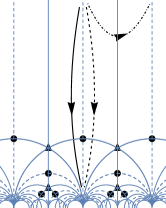
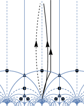
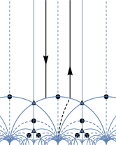
(a)		(b)		(c)

Figure 1: Paths $\tilde{\gamma}_{\tilde{g}_{\infty}}$, $\tilde{\gamma}_{\tilde{g}_{2}}$ and $\tilde{\gamma}_{\tilde{g}_{2}^{-1}}$ in the upper half plane $t\in{\cal H}$ are shown by dot-dashed, solid and dashed lines in (a) along with the boundaries of fundamental regions in thinner solid lines. The ${\rm PSL}_{2}\mathbb{Z}$ orbit of $t^{[0]}_{*}$ and $t^{[1]}_{*}$ are indicated by $\bullet$’s and $\blacktriangle$’s, respectively. The contours of integration for the period polynomials $P_{\tilde{g}_{2}}(t,f_{*})$ and $P_{\tilde{g}_{2}^{-1}}(t,f_{*})$ are drawn by solid and dashed lines, respectively, in (b). The contour for $P_{\tilde{g}_{2}}(t,f_{*})$ may be split into two segments (solid and dashed) in (c), and the integral over the dashed part of the contour may be further rewritten as an integral over the other solid line contour in (c).

It is not hard to find out numerically by using Mathematica that

$$P_{(\tilde{g}_{2})^{\pm 1}}(t,f_{*}) \;\simeq-0.610599i(t^{4}-1)\pm 0.5(t^{4}+2t^{2}+1)-1.5(t^{3}+t),$$ (94)

$$\;\simeq\frac{\zeta(3)}{(2\pi i)^{3}}\frac{(-252)}{2}(t^{4}-1)\pm\frac{t^{4}+2t+1}{2}-\frac{3}{2}(t^{3}+t).$$ (95)

Now, let us add the integration constants in the $(w-1)=5$-fold iterated integral, as in (75). The polynomial $Q(t)$ should be at most degree-4, but we set it to

$$Q(t)=\frac{0}{4!}t^{4}+\frac{d_{111}}{3!}t^{3}-\frac{a_{11}}{2}t^{2}-\frac{b_{1}}{24}t-\frac{\zeta(3)}{(2\pi i)^{3}}\frac{\chi}{2},$$ (96)

because we know for a Het–IIA dual vacuum that there must be a symplectic frame where the quartic term is absent in the prepotential (9). The relation (68, 78) determines the matrix $\Lambda_{\tilde{g}_{2}^{\pm 1}}$ as follows:

$$\Lambda_{(\tilde{g}_{2})^{\pm 1}}=\left(\begin{array}[]{cc|c}\pm 1+\frac{\zeta(3)}{(2\pi i)^{3}}(\chi+252)&\pm 1&\left(\frac{b_{1}}{24}-\frac{d_{111}}{6}-\frac{3}{2}\right)\\ \pm 1&\pm 1-\frac{\zeta(3)}{(2\pi i)^{3}}(\chi+252)&\left(\frac{b_{1}}{24}-\frac{d_{111}}{6}-\frac{3}{2}\right)\\ \hline\cr\left(\frac{b_{1}}{24}-\frac{d_{111}}{6}-\frac{3}{2}\right)&\left(\frac{b_{1}}{24}-\frac{d_{111}}{6}-\frac{3}{2}\right)&0\end{array}\right)+\mathbb{C}\widetilde{C}.$$ (100)

The $+\mathbb{C}\widetilde{C}$ ambiguity should be reduced to $+\mathbb{Z}\widetilde{C}$ (or dropped) because the ambiguity beyond $+\mathbb{Z}\widetilde{C}$ does not help making this $\Lambda_{\tilde{g}_{2}}$ matrix integer valued.

Before proceeding further, let us run a few checks with known results, to validate this method of computing the monodromy matrices. There is a branch with $\Lambda_{S}=\left\langle{+2}\right\rangle$ that has been studied extensively in the literature. That is the Heterotic construction known as the $ST$-model, whose Type IIA dual is for a Calabi–Yau threefold $M=(12)\subset\mathbb{P}^{4}_{[1:1:2:2:6]}$. This geometry indicates that $d_{111}=4$, $b_{1}=52$, and $\chi=-252$. When those values are substituted into (100), the monodromy matrix $M_{\tilde{g}_{2}^{-1}}=M(g_{2}^{-1},\Lambda_{\tilde{g}_{2}^{-1}})$ reproduces the monodromy matrix $(-S_{1})$ in [28], which was determined by using computations of the mirror manifold of $M$.

As a second check, remember that we have chosen the two paths $\tilde{\gamma}_{\tilde{g}_{2}}$ and $\tilde{\gamma}_{\tilde{g}_{2}^{-1}}$ both as lifts of

$$g_{2}=\left(\begin{array}[]{cc|c}&1&\\ 1&&\\ \hline\cr&&-1\end{array}\right)\in{\rm Isom}(\widetilde{\Lambda}_{S})$$ (104)

in a way they are for the inverse duality transformation of each other under the path composition law (36). Indeed, one can verify that both $M(g_{2},\Lambda_{\tilde{g}_{2}})\cdot M(g_{2},\Lambda_{\tilde{g}_{2}^{-1}})$ and $M(g_{2},\Lambda_{\tilde{g}_{2}^{-1}})\cdot M(g_{2},\Lambda_{\tilde{g}_{2}})$ are equal to the identity matrix by using (100, 104); we do not need to use a specific value for $\chi$, $d_{111}$ and $b_{1}$. One will also find that

$$\left(M(g_{2},\Lambda_{\tilde{g}_{2}})\right)^{2}=M({\bf 1},\Lambda_{\tilde{g}(X(v^{[0]}_{*}))}),\qquad\left(M(g_{2},\Lambda_{\tilde{g}_{2}^{-1}})\right)^{2}=M({\bf 1},-\Lambda_{\tilde{g}(X(v^{[0]}_{*}))}),$$ (105)

without substituting any value into $\chi$, $d_{111}$ and $b_{1}$.

Finally, one may define two lifts of the map $g_{3}:t\mapsto-1/(t+1)$. One is $\tilde{g}_{3}:=\tilde{g}_{2}\cdot\tilde{g}_{\infty}$ and the other $\tilde{g}_{3}^{\prime}:=\tilde{g}_{2}^{-1}\cdot\tilde{g}_{\infty}$; note that $g_{2}\cdot g_{3}=g_{\infty}$ and $g_{2}^{2}=1$ in ${\rm Isom}(\widetilde{\Lambda}_{S})$. The corresponding paths $\tilde{\gamma}_{\tilde{g}_{3}}$ and $\tilde{\gamma}_{\tilde{g}^{\prime}_{3}}$ are determined from (36) and are shown in Figure 2 (a).

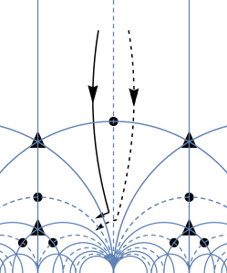
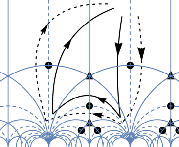
(a)		(b)

Figure 2: The paths $\tilde{\gamma}_{\tilde{g}_{3}}=(\tilde{\gamma}_{\tilde{g}_{\infty}})^{g_{2}}\circ\tilde{\gamma}_{\tilde{g}_{2}}$ for $\tilde{g}_{3}=\tilde{g}_{2}\cdot\tilde{g}_{\infty}$ and $\tilde{\gamma}_{\tilde{g}^{\prime}_{3}}=(\tilde{\gamma}_{\tilde{g}_{\infty}})^{g_{2}}\circ\tilde{\gamma}_{\tilde{g}_{2}^{-1}}$ for $\tilde{g}^{\prime}_{3}=\tilde{g}_{2}^{-1}\cdot\tilde{g}_{\infty}$ are drawn in the complex $t$ plane in (a) by the solid and dashed oriented lines, respectively. In the panel (b), the solid and dashed oriented lines are the paths (loops in fact) for $(\tilde{g}_{3})^{3}$ and $(\tilde{g}^{\prime}_{3})^{3}$, respectively. For more information, see the caption of Figure 1.

A straightforward matrix computation confirms that

$$(M_{\tilde{g}_{3}})^{3} \;=(M_{\tilde{g}_{2}}\cdot M_{\tilde{g}_{\infty}})^{3}=M({\bf 1},(d_{111}/2-2)\widetilde{C}),$$ (106)

$$(M_{\tilde{g}^{\prime}_{3}})^{3} \;=(M_{\tilde{g}_{2}^{-1}}\cdot M_{\tilde{g}_{\infty}})^{3}=M({\bf 1},\Lambda^{\prime}),$$ (107)

$$\Lambda^{\prime}=-\Lambda_{\tilde{g}(X(v^{[0]}_{*}))}-\Lambda_{\tilde{g}(X(v^{[0]}_{**}))}-\Lambda_{\tilde{g}(X(v^{[0]}_{***}))}+(d_{111}/2-2)\widetilde{C};$$ (108)

here, $v^{[0]}_{**}=(1,2,2)\in\widetilde{\Lambda}_{S}^{\vee}$ and $v^{[0]}_{***}=(2,1,2)$, with the corresponding states becoming massless at $t^{[0]}_{**}=(-1+i)/2$ and $t^{[0]}_{***}=(-1+i)$, respectively. It is appropriate that the relations (106, 108) hold without including monodromy contributions from the ${\rm PSL}_{2}\mathbb{Z}$ orbit of $t^{[1]}_{*}$ on the right-hand sides (see Figure 2 (b)), because the computation (95) is for $f_{*}$ in (91), which is for $n_{1/2}=0$,

Note that we have tools to compute the monodromy matrices $M_{\tilde{g}}$ from first principle, using numerical evaluation of the period polynomials. It is not that the relations such as (105, 106, 108) are imposed to constrain $\Lambda_{\tilde{g}}$ that is otherwise intractable; we computed the matrices $\Lambda_{\tilde{g}}$ from first principle and expressed them in terms of the (implicit $n_{1/2}=0$ and) integration constants $d_{111}$, $b_{1}$ and $\chi$; the relations (105, 106, 108) are satisfied automatically, as explained in (79–81).

Let us now go back to the program of imposing the integrality of the monodromy matrices to narrow down theoretically possible choices of the classification invariants. Demanding that all the matrix entries in (100) are integers, we obtain conditions that are independent from (88). A common solution to those conditions is parametrized as

$$\chi=-252,\quad d_{111}=2D,\quad b_{1}=8D+36+24B,\quad a_{11}=A,$$ (109)

for $D,A,B\in\mathbb{Z}$. The first two conditions impose extra conditions on the classification invariants $(n_{0},n_{1/2},b_{\cal R})=(-2,0,b_{\cal R})$. The required value $\chi=-252$ here is the same as the value $[-c_{0}(0)]_{n_{1/2}=0}=-252$ determined in an independent reasoning (11), so the extra condition is satisfied (see also section 5). The condition that $d_{111}$ is even (for $n_{1/2}=0$) implies that only

$$b_{\cal R}\in 2\mathbb{Z}$$ (110)

are for branches of theoretically consistent Het–IIA dual moduli space.

We are also ready to compare the two parameters of the 4d effective theory, $(b_{1})_{+24\mathbb{Z}}$ and $(c_{2})_{1}$ modulo $24\mathbb{Z}$ (not just mod $12\mathbb{Z}$ as in (90)).

$$(b_{1})_{+24\mathbb{Z}}-(c_{2})_{1}\equiv\left(36+16-4b_{\cal R}\right)-\left(52-4b_{\cal R}\right)\equiv 0.$$ (111)

So, for any branch of Het–IIA dual vacua with integral monodromy matrices, we have seen that the two parameters $(b_{1})_{+24\mathbb{Z}}$ and $(c_{2})_{1}$ yield one common value that is interpreted as $\int_{M}c_{2}(TM)D_{a=1}$ if the branch is given by a non-linear sigma model with the target space $M$ in the Type IIA description.

Now, the conditions (44) is read precisely as Wall’s condition for (necessary and) sufficient condition for a diffeomorphism class $[M]$ of real 6-manifolds $M$ to exist, with the trilinear intersection form on $H^{2}(M;\mathbb{Z})$ and the 2nd Chern class in $H^{4}(M;\mathbb{Z})$ characterized by $(C_{11},d_{111})$ and $(24,(c_{2})_{1})$. The conditions (45, 111) are equal to the additional conditions (16, 17) for the central charge of 4d ${\cal N}=2$ supersymmetry from D-branes appropriate in a phase of non-linear sigma model description. So, we have seen that all the branches of theoretically consistent Het–IIA dual moduli space with $\Lambda_{S}=\left\langle{+2}\right\rangle$ and $n_{1/2}=0$ contain phases described by a non-linear sigma model in the Type IIA language.

Now, three (or possibly more) distinct branches of moduli space remain (among those with $\Lambda_{S}=\left\langle{+2}\right\rangle$ and $n_{1/2}=0$). The integer parameters $A$ and $B$ differ by $+\mathbb{Z}$ do not lead to distinct spectra of electrically/magnetically charged 4d ${\cal N}=2$ BPS states (note that $\Delta a_{11}\in\mathbb{Z}$ and $\Delta b_{1}\in 24\mathbb{Z}$ and remember (10)). $\Delta D\in 3\mathbb{Z}$ also fall into the ambiguity in (10). So, $D_{+3\mathbb{Z}}\in\{2,1,0\}_{+3\mathbb{Z}}$ (or equivalently $(b_{\cal R})_{+6\mathbb{Z}}\in\{0,2,4\}_{+6\mathbb{Z}}$) label the three branches. Calabi–Yau threefolds for those three branches are known in the literature [29, 27].

3.2.3 The Cases $n_{1/2}=1,2,3,4$

It is straightforward to employ the same method to determine the monodromy matrix $M_{\tilde{g}_{2}}$ for the cases with $\Lambda_{S}=\left\langle{+2}\right\rangle$ and $n_{1/2}>0$. The weight-6 automorphic form $f_{*}$ in (71) under ${\rm PSL}_{2}\mathbb{Z}$ must be determined uniquely for individual $n_{1/2}\in\{0,1,2,3,4\}$, and it should be of the form

$$f_{*}(t) \;=\frac{1}{(2\pi i)^{3}}\frac{aE_{4}^{9}+bE_{4}^{6}E_{6}^{2}+cE_{4}^{3}E_{6}^{4}+dE_{6}^{6}}{E_{4}^{3}E_{6}^{3}}$$ (112)

for some coefficients $a,b,c,d$ because $\partial_{t}^{2}{\cal F}^{(1)}$ (and hence the three-fold integral of $f_{*}$) should have logarithmic singularity at $t\simeq t^{[0]}_{*}=i$ (where $E_{6}(t)\simeq 0$) and also at $t\simeq t^{[1]}_{*}=e^{2\pi i/3}$ (where $E_{4}(t)\simeq 0$). The coefficients $a,b,c,d$ may, in principle, be determined by exploiting (72, 53); we demand instead that the $e^{2\pi it}$ series expansion of $f_{*}$ agrees with the $e^{2\pi it}$ series expansion of $(2\pi i)^{-5}\partial_{t}^{5}{\cal F}^{(1)}$, where the coefficients of the latter are determined by $n_{w,k=0}=c_{\gamma}((w,w)/2)$’s (see §A.2). It turns out that

$$a=2,\quad b=-\frac{23}{9},\quad c=\frac{5+2n_{1/2}}{9},\quad d=-\frac{2n_{1/2}}{9}.$$ (113)

The period polynomial $P_{\tilde{g}_{2}}(t;f_{*})$ can be evaluated numerically for individual $n_{1/2}\in\{1,2,3,4\}$, just like we have done for the case $n_{1/2}=0$. The results are fitted very well by the formula

$$P_{\tilde{g}_{2}}(t;f_{*}) \;\simeq\frac{\zeta(3)}{(2\pi i)^{3}}\frac{(-252+56n_{1/2})}{2}(t^{4}-1)+\frac{t^{4}+2t+1}{2}+\left(-\frac{3}{2}+\frac{n_{1/2}}{4}\right)(t^{3}+t).$$ (114)

This is combined with the contributions from the integration constant terms (96) to determine (78), and hence the matrix $\Lambda_{\tilde{g}_{2}}$.

$$\Lambda_{\tilde{g}_{2}} \;=\left(\begin{array}[]{cc|c}1+\frac{\zeta(3)}{(2\pi i)^{3}}X_{0}&1&\left(\frac{b_{1}}{24}-\frac{d_{111}}{6}-\frac{3}{2}+\frac{n_{1/2}}{4}\right)\\ 1&1-\frac{\zeta(3)}{(2\pi i)^{3}}X_{0}&\left(\frac{b_{1}}{24}-\frac{d_{111}}{6}-\frac{3}{2}+\frac{n_{1/2}}{4}\right)\\ \hline\cr\left(\frac{b_{1}}{24}-\frac{d_{111}}{6}-\frac{3}{2}+\frac{n_{1/2}}{4}\right)&\left(\frac{b_{1}}{24}-\frac{d_{111}}{6}-\frac{3}{2}+\frac{n_{1/2}}{4}\right)&0\end{array}\right)+\mathbb{Z}\widetilde{C},$$ (118)

where

$$X_{0}:=\chi+252-56n_{1/2}.$$ (119)

When we use the value of $\chi$ determined by the reasoning reviewed in (11) (see also §A.2), the combination $X_{0}$ vanishes for all $n_{1/2}$.

The value of $(b_{1})_{+24\mathbb{Z}}$ is determined when we demand that all the entries of the matrix $\Lambda_{\tilde{g}_{2}}$ be integers. This condition on $b_{1}$ mod $24\mathbb{Z}$ and the conditions (88) combined imposes one condition $d_{111}-n_{1/2}\in 2\mathbb{Z}$, or equivalently

$$b_{\cal R}\in 2\mathbb{Z}_{\geq 0}$$ (120)

on the classification invariant, besides determining $(b_{1})_{+24\mathbb{Z}}$ and $(a_{11})_{+\mathbb{Z}}$. One also finds that

$$(b_{1})_{+24\mathbb{Z}}=52-4b_{\cal R}-10n_{1/2}+24\mathbb{Z}=(c_{2})_{1}+24\mathbb{Z}$$ (121)

by using (84, 85).

We have therefore seen that both $(b_{1})_{+24\mathbb{Z}}$ and $(c_{2})_{1}$ yield one common thing that can be interpreted as the 2nd Chern class of the target space in the Type IIA language. Now, the conditions (44) is read as the sufficient conditions for existence of a diffeomorphism class $[M]$ of real 6-dimensional manifolds whose trilinear intersection form and the 2nd Chern class on $H^{2}(M;\mathbb{Z})$ agree with what we compute from the data $\Lambda_{S}$, $\{\Phi\}$ and $b_{\cal R}$. It is reasonable to conclude (cf footnote 23) that all those branches with $\Lambda_{S}=\left\langle{+2}\right\rangle$, $n_{1/2}\in\{0,1,2,3,4\}$ and $\mathbb{Z}$-valued monodromy matrices have a region described by the non-linear sigma model in the Type IIA language, with $M$ the target space. Table 1 of Ref. [29] shows that there is a known construction for Calabi–Yau threefolds $M$ whose diffeomorphism classes $[M]$ correspond to $n_{1/2}=1$, $b_{\cal R}+6\mathbb{Z}=\{0,2\}_{+6\mathbb{Z}}$, $n_{1/2}=2$, $b_{\cal R}+6\mathbb{Z}=\{0,2\}_{+6\mathbb{Z}}$, $n_{1/2}=3$, $b_{\cal R}+6\mathbb{Z}=\{0\}_{+6\mathbb{Z}}$. At this moment, it is not clear whether a geometry with $(n_{1/2},b_{\cal R}+6\mathbb{Z})=(1,4_{+6\mathbb{Z}}),(2,4_{+6\mathbb{Z}}),(3,2_{+6\mathbb{Z}}),(3,4_{+6\mathbb{Z}}),(4,\{0,2,4\}_{+6\mathbb{Z}})$ is simply not within the range of parameters of the toric ambient space scanned in [29], or not within the category of complete intersection of a toric variety, or such a geometry does not exist for a reason we do not understand yet.

4 The Case $\Lambda_{S}=U$

As another example, let us work on the case $\Lambda_{S}=U$. Historically, the relevance of an automorphic form $f_{*}$ to the monodromy matrices has been observed in this $\Lambda_{S}=U$ case for the first time [2, 3], so the following presentation is inevitably very close to what is written in the literature. What we do here is to be faithful to the first principle calculation of the monodromy matrices to narrow down the theoretically possible choices of classification invariants, instead of finding relevance of $f_{*}$ in a string vacuum with a known construction.

Let us start off by reviewing known things. On the lattice $\Lambda_{S}=U$, let us choose a basis $\{e_{\rho},e_{u}\}$ so that $(e_{\rho},e_{\rho})=(e_{u},e_{u})=0$ and $(e_{\rho},e_{u})=1$. The moduli space $D(\widetilde{\Lambda}_{S})$ is parametrized by $\mho=(1,(t,t)/2,t)^{T}=(1,\rho u,\rho,u)^{T}$, where $t=e_{\rho}\rho+e_{u}u\in\Lambda_{S}\otimes\mathbb{C}$. The lattice isometry group ${\rm Isom}(\widetilde{\Lambda}_{S})$ is (e.g., [30, 31])

$$\left({\rm PSL}_{2}^{(\rho)}\mathbb{Z}\times{\rm PSL}_{2}^{(u)}\mathbb{Z}\right)\rtimes(\mathbb{Z}_{2}\left\langle{\sigma}\right\rangle\times\mathbb{Z}_{2}(-1)_{\rho u})\times\mathbb{Z}_{2}(-id),$$ (122)

where ${\rm PSL}_{2}^{(\rho)}\mathbb{Z}$ and ${\rm PSL}_{2}^{(u)}\mathbb{Z}$ act on $D(\widetilde{\Lambda}_{S})=\{(\rho,u)\in\mathbb{C}\;|\;{\rm Im}(\rho){\rm Im}(u)>0\}$ as linear fractional transformations on $\rho$ and $u$, respectively, and $(-1)_{\rho u}:(\rho,u)\mapsto(-\rho,-u)$. The map $\sigma$ brings $(\rho,u)$ to $(\rho^{\sigma},u^{\sigma})=(u,\rho)$. The discriminant group $G_{S}$ is trivial for $\Lambda_{S}=U$, and so is the group ${\rm Isom}(G_{S},q_{S})$. So, all the elements in ${\rm Isom}(\widetilde{\Lambda}_{S})$ lifts to isometries of ${\rm Isom}({\rm II}_{4,20})$ for the embedding $\widetilde{\Lambda}_{S}={\rm II}_{2,2}\hookrightarrow{\rm II}_{2,2}\oplus{\rm II}_{2,18}={\rm II}_{4,20}$. For this reason, we will demand in this article that all the elements $g\in{\rm Isom}(\widetilde{\Lambda}_{S})$ should have a lift duality transformation $\tilde{g}$ whose monodromy matrix is $\mathbb{Z}$-valued.

Before starting to work out the monodromy matrices, let us also quote the results on classification invariants for the case $\Lambda_{S}=U$. The invariant $\{\Phi\}$ is the unique scalar valued weight $(11-\rho/2=10)$ modular form starting with $n_{\gamma=0}=-2$, which is $\Phi=-2E_{4}E_{6}$. One more classification invariant is

$$b_{\cal R}\in 2^{-1}\mathbb{Z}_{\geq 0}.$$ (123)

With this invariant, the parameters of the effective theory in the ${\rm Im}(u)>{\rm Im}(\rho)$ phase are given by [12, 13, 10]

$$d_{\rho\rho u} \;=n^{\prime}-2+2\delta n_{\rho},\qquad d_{\rho uu}=n^{\prime}+2\delta n_{u},\qquad d_{\rho\rho\rho}=2,\qquad d_{uuu}=0,$$ (124)

$$(c_{2})_{\rho} \;=12(2+n^{\prime})-4+24\delta n_{\rho},\qquad(c_{2})_{u}=12(2+n^{\prime})+24\delta n_{u};$$ (125)

Here, $n^{\prime}:=2-b_{\cal R}/6$.

4.1 Analysis on the $\Lambda_{S}=U$ Case

Now, let us choose a base point of paths in a connected part ${\cal H}_{\rho}\times{\cal H}_{u}$ of the covering space $D(\widetilde{\Lambda}_{S})$,

$$t_{0}^{(u)}=(\rho_{0}^{(u)},u_{0}^{(u)})\simeq(i{\rm~{}large~{}positive~{}finite},\;+i\infty);$$ (126)

$\rho_{0}^{(u)}$ is chosen to be purely imaginary with the imaginary part finite but much larger than 1. All the loci of extra massless fields are [3] of the form of $\rho=u^{g}$ for some $g\in{\rm PSL}_{2}^{(u)}\mathbb{Z}$, and form a single orbit under ${\rm Isom}(\widetilde{\Lambda}_{S})$. Monodromy matrices for loops in the covering space is completely understood, so we are left to choose a set of generators $\{g_{i}\}$ of $[{\rm PSL}_{2}^{(\rho)}\mathbb{Z}\times{\rm PSL}_{2}^{(u)}\mathbb{Z}]\rtimes\mathbb{Z}_{2}\left\langle{\sigma}\right\rangle$, find one lift $\tilde{g}_{i}$ (and $\tilde{\gamma}_{\tilde{g}_{i}}$) for each $g_{i}$ and compute the matrix $M_{\tilde{g}_{i}}$. As a set of generators, we choose $\{g_{\infty(u)}^{\pm 1},g_{\infty(\rho)}^{\pm 1},\sigma,g_{2(u)}^{\pm 1}\}$, where $g_{\infty(u)}$ and $g_{2(u)}$ keep $\rho$ invariant and act on $u$ as $u\mapsto u+1$ and $u\mapsto-1/u$, respectively. Similarly, $g_{\infty(\rho)}:\rho\mapsto\rho+1$.

To specify one lift $\tilde{g}_{i}$ for each $g_{i}$, we describe the corresponding path $\tilde{\gamma}_{\tilde{g}_{i}}$, as follows. The paths $\tilde{\gamma}_{\tilde{g}_{\infty(\rho)}}$ and $\tilde{\gamma}_{\tilde{g}_{\infty(u)}}$ both start from $t_{0}^{(u)}$, and have $\Delta\rho=+1$ for fixed $u=u_{0}^{(u)}$ and $\Delta u=+1$ for fixed $\rho=\rho_{0}^{(u)}$, respectively, to reach the endpoint $(t_{0}^{(u)})^{g_{\infty(\rho)}}$ and $(t_{0}^{(u)})^{g_{\infty(u)}}$, respectively. The path $\tilde{\gamma}_{2(u)}$ starts from $t_{0}^{(u)}$, and moves in the $u$-plane down the imaginary axis (and fixed $\rho=\rho_{0}^{(u)}$) to $u=-1/(u_{0}^{(u)})$, while avoiding $u=\rho_{0}^{(u)}$ by detouring into the 2nd quadrant in the $u$-plane. Finally, the path $\tilde{\gamma}_{\tilde{\sigma}}$ [resp. $\tilde{\gamma}_{\tilde{\sigma}^{-1}}$] starts from $t_{0}^{(u)}$ and ends at $(t_{0}^{(u)})^{\sigma}=(u_{0}^{(u)},\rho_{0}^{(u)})$, avoiding the $u=\rho$ singularity on the way by temporarily setting ${\rm Re}(\rho)$ to be positive [resp. negative]; see Figure 3 (a).

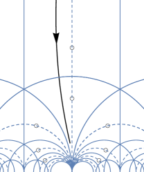
(a)		(b)

Figure 3: The paths $\tilde{\gamma}_{\tilde{\sigma}}$ and $\tilde{\gamma}_{\tilde{\sigma}^{-1}}$ are shown by the solid and dashed curves, respectively, in the ${\rm Im}(u)=0$ slice of the $(\rho,u)\in\mathbb{C}^{2}$ space in (a); the $u=\rho$ singularity is shown by the dot-dashed line. The panel (b) shows the path $\tilde{\gamma}_{\tilde{g}_{2(u)}}$ in the $\rho=\rho_{0}^{(u)}$ slice of the $(\rho,u)$ parameter space. The singularity at $u\in{\rm PSL}_{2}\mathbb{Z}\cdot\rho_{0}^{(u)}$ are marked by the open circles.

The corresponding duality transformation (analytic continuation of the section $\Pi=(X,F)^{T}$ along those paths) are denoted by $\tilde{g}_{\infty,\rho}$, $\tilde{g}_{\infty,u}$, $\tilde{g}_{2,u}$, and $\tilde{\sigma}^{\pm 1}$, respectively.

The monodromy matrices for $\tilde{g}_{\infty(\rho)}$ and $\tilde{g}_{\infty(u)}$ are given by $g_{\infty(\rho)}$, $g_{\infty(u)}$ and (42). The effective theory parameters are subject to the conditions (44, 45), or more explicitly,

$$d_{\rho\rho\rho},\quad d_{\rho\rho u},\quad d_{\rho uu},\quad d_{uuu}\in\mathbb{Z},$$ (127)

$$(a_{\rho\rho})_{+\mathbb{Z}}=(d_{\rho\rho\rho}/2)+\mathbb{Z},\quad(a_{uu})_{+\mathbb{Z}}=(d_{uuu}/2)+\mathbb{Z},$$ (128)

$$(a_{\rho u})_{+\mathbb{Z}}=d_{\rho\rho u}/2+\mathbb{Z},$$ (129)

$$d_{\rho\rho u}\in d_{\rho uu}+2\mathbb{Z},$$ (130)

$$2d_{uuu}+b_{u}\in 12\mathbb{Z},\qquad 2d_{\rho\rho\rho}+b_{\rho}\in 12\mathbb{Z}.$$ (131)

Those conditions imply that the classification invariant $b_{\cal R}$ can take values only in

$$b_{\cal R}\in 6\mathbb{Z}_{\geq 0}$$ (132)

in a branch of theoretically consistent Het–IIA dual moduli space, not $2^{-1}\mathbb{Z}_{\geq 0}$. The values of $(a_{\rho\rho})_{+\mathbb{Z}}$ and $(a_{uu})_{+\mathbb{Z}}$ are also fixed, when combined with the parametrization (124). The values of $(b_{\rho})_{+24\mathbb{Z}}$ and $(b_{u})_{+24\mathbb{Z}}$ are determined only modulo $+12\mathbb{Z}$. At this level of precision,

$$(b_{\rho})_{+12\mathbb{Z}}=(-2d_{\rho\rho\rho})_{+12\mathbb{Z}}=-4+12\mathbb{Z}, \qquad(c_{2})_{\rho}\equiv-4\quad({\rm mod~{}}12\mathbb{Z}),$$ (133)

$$(b_{u})_{+12\mathbb{Z}}=(-2d_{uuu})_{+12\mathbb{Z}}=12\mathbb{Z}, \qquad(c_{2})_{u}\equiv 0\quad({\rm mod~{}}12\mathbb{Z}).$$ (134)

So, we are left with $(b_{a})_{+24\mathbb{Z}}\equiv(c_{2})_{a}$ mod 24, or $(c_{2})_{a}+12$ mod 24, chosen individually for $a=\rho$ and $a=u$.

The monodromy representation matrices $M_{\tilde{\sigma}^{\pm 1}}=M(\sigma,\Lambda_{\tilde{\sigma}^{\pm 1}})$ are given by computing the analytic continuation of ${\cal F}^{(1)}$ from $t_{0}=(\rho^{(u)}_{0},u^{(u)}_{0})$ to $t_{0}^{\sigma}=(u_{0}^{(u)},\rho_{0}^{(u)})$ along the paths $\tilde{\gamma}_{\tilde{\sigma}^{\pm 1}}$. In addition to the polynomial terms of ${\cal F}^{(1)}$, one more term $c(-1){\rm Li}_{3}(e^{2\pi i(u-\rho)})/(2\pi i)^{3}$ in ${\cal F}^{(1)}$ contributes to ${\cal F}^{(1)}(t^{\tilde{\sigma}^{\pm 1}})-{\cal F}^{(1)}(t)$ in (47). Using

$$\frac{\left[{\rm Li}_{3}(e^{2\pi i(u-\rho)})\right]_{{\rm along~{}}\tilde{\gamma}_{\tilde{\sigma}^{\pm 1}}}}{(2\pi i)^{3}}-\frac{{\rm Li}_{3}(e^{2\pi i(u-\rho)})}{(2\pi i)^{3}}=\frac{1}{3!}\left[(u-\rho)^{3}\mp\frac{3}{2}(u-\rho)^{2}+\frac{1}{2}(u-\rho)\right]$$ (135)

and $c(-1)=-2$ (see §A.2), one finds that

$${\cal F}^{(1)}(t^{\tilde{\sigma}^{\pm 1}})-{\cal F}^{(1)}(t) \;=\frac{\pm 1-a_{\rho\rho}+a_{uu}}{2}u^{2}+\frac{\pm 1+a_{\rho\rho}-a_{uu}}{2}\rho^{2}\mp\rho u+\frac{4+b_{\rho}-b_{u}}{24}(\rho-u);$$ (136)

cubic terms cancel when we use (124). The monodromy matrices $M_{\tilde{\sigma}}=M(\sigma,\Lambda_{\tilde{\sigma}})$ and $M_{\tilde{\sigma}^{-1}}=M(\sigma,\Lambda_{\tilde{\sigma}^{-1}})$ are now determined by (47).

$$\sigma=\left[\begin{array}[]{cc|cc}1&&&\\ &1&&\\ \hline\cr&&&1\\ &&1&\end{array}\right],\quad\Lambda_{\tilde{\sigma}^{\pm 1}}=\left[\begin{array}[]{cc|cc}0&0&\frac{4+b_{\rho}-b_{u}}{24}&-\frac{4+b_{\rho}-b_{u}}{24}\\ 0&0&0&0\\ \hline\cr&&\pm 1+a_{\rho\rho}-a_{uu}&\mp 1\\ &&\mp 1&\pm 1-a_{\rho\rho}+a_{uu}\end{array}\right]+\mathbb{Z}\widetilde{C};$$ (145)

the lower-left corner of the symmetric matrices $\Lambda_{\tilde{\sigma}^{\pm 1}}$ are omitted just to save space. The two matrices automatically satisfy the relations (cf footnotes 9, 22 and 27)

$$(M_{\tilde{\sigma}^{\pm 1}})^{2}\in M({\bf 1},\pm\Lambda_{\tilde{g}(X(v_{\rho u}))})\cdot(M_{D})^{n},\qquad n\in\mathbb{Z},$$ (146)

where $\pm v_{\rho u}=\pm(0,0,-1,1)\in\widetilde{\Lambda}_{S}^{\vee}$ are the charges of the states that become massless at $u=\rho$.

By demanding that the matrices $\Lambda_{\tilde{\sigma}^{\pm 1}}$ are $\mathbb{Z}$-valued, we obtain one more condition.

$$(b_{\rho})_{+24\mathbb{Z}}+4=(b_{u})_{+24\mathbb{Z}};$$ (147)

two choices are left, $b_{\rho}+4\equiv b_{u}\equiv 0$ mod 24 and $\equiv 12$ mod 24.

Finally, let us determine the monodromy matrix of the duality transformation $\tilde{g}_{2(u)}$. To find out how ${\cal F}^{(1)}(\rho_{0}^{(u)},-1/u_{0}^{(u)})$ is related to ${\cal F}^{(1)}(\rho_{0}^{(u)},u_{0}^{(u)})$, we use numerical evaluation of the period polynomial.

For $g_{(u)}\in{\rm PSL}_{2}^{(u)}\mathbb{Z}$ mapping $u\mapsto(au+b)/(cu+d)$, the relation (47) reads

$$(cu+d)^{2}{\cal F}^{(1)}(\rho,u^{\tilde{g}_{(u)}})={\cal F}^{(1)}(\rho,u)+\frac{1}{2}\mho(\rho,u)^{T}\Lambda_{\tilde{g}_{(u)}}\mho(\rho,u).$$ (148)

The 3rd derivative of ${\cal F}^{(1)}$ with respect to $u$ transforms as a modular form under ${\rm PSL}_{2}^{(u)}\mathbb{Z}$ of weight $(w=+4)$ [2], so we set

$$f_{*}(u;\rho):=\frac{1}{(2\pi i)^{3}}\partial_{u}^{3}{\cal F}^{(1)}(\rho,u).$$ (149)

This modular form $f_{*}(u;\rho)$ is determined uniquely by the unique $\Phi$ (independent of the classification invariant $b_{\cal R}\in 6\mathbb{Z}$), because [3, (2.15)] (note also (53))

$$-\rho_{2}^{2}[u_{2}^{-2}\partial_{u}u_{2}^{2}]\partial_{u}\bar{\partial}_{\bar{\rho}}\left(\hat{K}^{(0)a\bar{b}}G^{(1)}_{a\bar{b}}\right)=\cdots=\frac{i}{2}\partial_{u}^{3}{\cal F}^{(1)}(\rho,u)=\frac{i}{2}(2\pi i)^{3}f_{*}(u;\rho).$$ (150)

It is known [2, 3] that this uniquely determined $f_{*}(u;\rho)$ for all the $\Lambda_{S}=U$ cases is of the form (cf [32])

$$f_{*}(u;\rho) \;=\frac{1}{(2\pi i)^{3}}\frac{-i}{\pi}\frac{j_{u}(u)}{j(u)-j(\rho)}\frac{j(\rho)}{j(u)}\frac{j_{u}(u)}{j_{\rho}(\rho)}\frac{j(\rho)-j(i)}{j(u)-j(i)},$$ (151)

$$\;=\frac{1}{(2\pi i)^{3}}\frac{2}{j(\rho)-j(u)}E_{4}(u)\frac{E_{4}E_{6}}{\eta^{24}}(\rho).$$ (152)

Note that $f_{*}(u,\rho)$ for a fixed value of $\rho$ has the behavior $f_{*}(u)\simeq e^{2\pi iu}\times({\rm const}.)+{\cal O}(e^{2\pi i2u})$ at large ${\rm Im}(u)$, so this is a cusp form of weight $(w=4)$ with poles (at $u=\rho$ and its ${\rm PSL}_{2}\mathbb{Z}$ images) in the upper half plane of $u$.

The part of the prepotential ${\cal F}^{(1)}(\rho,u)$ should be reproduced from $f_{*}(u;\rho)$ by a $(w-1)=3$-fold integral with respect to the coordinate $2\pi iu$. The indefinite integral (the Eichler integral) $I[u;f_{*},\tilde{\gamma},\rho]=F_{\rm Eich}(u;f_{*},\tilde{\gamma},\rho)$ starting from $u=u_{0}^{(u)}\simeq i\infty$ converges (see the review in section 3.1.3), and makes sense uniquely when the path $\tilde{\gamma}$ stops at ${\rm Im}(u)\gg{\rm Im}(\rho)$; for this reason, the $(w-1)$-fold integral (75) is ready for an easy interpretation in the ${\rm Im}(u)>{\rm Im}(\rho)$ phase. The integration constant terms $Q(u;\rho)$ in (75) is a polynomial of $u$ of at most degree $(w-2)=2$, which should be of the form

$$Q(u;\rho) \;=\left(\frac{d_{\rho uu}}{2}\rho-\frac{a_{uu}}{2}\right)u^{2}+\left(\frac{d_{\rho\rho u}}{2}\rho^{2}-a_{\rho u}\rho-\frac{b_{u}}{24}\right)u$$ (153)

$$\quad+\left(\frac{d_{\rho\rho\rho}}{6}\rho^{3}-\frac{a_{\rho\rho}}{2}\rho^{2}-\frac{b_{\rho}}{24}-\frac{\zeta(3)}{(2\pi i)^{3}}\frac{\chi}{2}+\sum_{n\geq 1}\frac{n_{(n,0),0}}{(2\pi i)^{3}}{\rm Li}_{3}(e^{2\pi i\rho n})\right).$$

Neither the Eichler integral $F_{\rm Eich}(u;f_{*},\tilde{\gamma},\rho)$ nor the integration constant terms give rise to the $u^{3}$ term in the ${\rm Im}(u)>{\rm Im}(\rho)$ phase, but that is consistent with the known parametrization $d_{uuu}=0$ (for ${\rm Im}(u)>{\rm Im}(\rho)$) by the classification invariants (see (124)).

Now let us determine $\Lambda_{\tilde{g}_{2(u)}}$ in the monodromy matrix $M_{\tilde{g}_{2(u)}}=M(g_{2(u)},\Lambda_{\tilde{g}_{2(u)}})$, by using (148, 78). We evaluated the period polynomial $P_{\tilde{g}_{2(u)}}(u;f_{*},\rho)$ for several values of $\rho$ by carrying out numerical integrals just like in the $\Lambda_{S}=\left\langle{+2}\right\rangle$ cases. It turns out that there is a nice fitting formula for the numerical integrals. The $u$ and $(u^{2}+1)$ terms in the polynomial $P_{\tilde{g}_{2(u)}}(u;f_{*},\rho)$ are

$$[P_{\tilde{g}_{2(u)}}(u;f_{*},\rho)]_{u,(u^{2}+1)} \;\simeq-2(\rho^{2}+1)u+\frac{\rho^{2}+1}{2}(u^{2}+1),$$ (154)

and the $(u^{2}-1)$ term satisfies

$$[P_{\tilde{g}_{2(u)}}(u;f_{*},\rho)]_{(u^{2}-1)} \;+(u^{2}-1)\left[\frac{\zeta(3)}{(2\pi i)^{3}}\frac{480}{2}+\frac{480}{(2\pi i)^{3}}\sum_{n\geq 1}{\rm Li}_{3}(e^{2\pi i\rho n})\right]$$

$$\;\simeq(u^{2}-1)\left[\frac{5}{6}\rho-\frac{1}{3}\rho^{3}\right],$$ (155)

where we have used $\chi=-c(0)=-480$ and $n_{(n,0),0}=c(n\cdot 0)=c(0)=480$ from (11) (see §A.2). So, the deviation (78) from the modular transformation property for ${\cal F}^{(1)}(\rho,u)$ is now purely polynomial in both $\rho$ and $u$. Moreover, the $(u^{2}-1)\rho^{3}$ terms cancel because $d_{\rho\rho\rho}=2$ in (124). So, we obtain

$$\Lambda_{\tilde{g}_{2(u)}}=\left[\begin{array}[]{cc|cc}1-a_{uu}&0&\frac{b_{\rho}+12d_{\rho uu}-20}{24}&-2+\frac{b_{u}}{12}\\ &1-a_{\rho\rho}&-2-d_{\rho\rho u}&-\frac{b_{\rho}+12d_{\rho uu}-20}{24}\\ \hline\cr&&1+a_{\rho\rho}&2a_{\rho u}\\ &&&1+a_{uu}\end{array}\right]+\mathbb{Z}\widetilde{C}.$$ (160)

Almost all the entries of the matrix $\Lambda_{\tilde{g}_{2(u)}}$ are automatically integers based on the conditions that have been derived. One new condition is obtained, however, which determines $(b_{\rho})_{+24\mathbb{Z}}$ uniquely, and consequently also determines $(b_{u})_{+24\mathbb{Z}}$ because of (147).

$$(b_{\rho})_{+24\mathbb{Z}}=20+12n^{\prime}+24\mathbb{Z}, \qquad(c_{2})_{\rho}\equiv 20+12n^{\prime}\quad({\rm mod~{}}24\mathbb{Z}),$$ (161)

$$(b_{u})_{+24\mathbb{Z}}=(b_{\rho})_{+24\mathbb{Z}}, \qquad(c_{2})_{u}\equiv(c_{2})_{\rho}+4\quad({\rm mod~{}}24\mathbb{Z}).$$ (162)

So the uniquely determined $(b_{a})_{+24\mathbb{Z}}$’s agree with $(c_{2})_{a}$ mod $24\mathbb{Z}$.

Now that we have confirmed that $(b_{a})_{+24\mathbb{Z}}$ and $(c_{2})_{a}$’s allow a common thing interpreted as the 2nd Chern class, we can regard the conditions (127, 130, 131) as Wall’s necessary and sufficient condition for existence of a diffeomorphism class $[M]$ of real 6-dimensional manifolds, with the trilinear intersection of $H^{2}(M;\mathbb{Z})$ and the 2nd Chern class given by $d_{abc}$ and $(c_{2})_{a}$, respectively. In any one of the branches of Het–IIA moduli space with $\Lambda_{S}=U$, therefore, there is a region described by a non-linear sigma model with the target space $M$ in the Type IIA language (cf footnote 23). The properties (128, 129) and $(b_{a})\equiv(c_{2})_{a}$ mod 24 guarantee that necessary conditions (16, 17) for D-brane central charges in a geometric phase are satisfied.

Those branches of moduli space with $\Lambda_{S}=U$ come with the unique $\Phi$ and the invariant $b_{\cal R}\in 6\mathbb{Z}_{\geq 0}$. Two $b_{\cal R}$’s that differ by $12\mathbb{Z}$ (i.e., two $n^{\prime}$’s that differ by $2\mathbb{Z}$) result in an identical spectrum of 4d ${\cal N}=2$ BPS dyons. The two branches with distinct dyon spectra, one with $b_{\cal R}\equiv 0$ (12) and the other with $b_{\cal R}\equiv 6$ (12) (i.e., even $n^{\prime}$ and odd $n^{\prime}$) have known descriptions both in the Type IIA and Heterotic languages. In Type IIA, the corresponding Calabi–Yau threefold is the elliptic fibration over the Hirzebruch surface $F_{0}$ (or $F_{2}$) and $F_{1}$, respectively. In Heterotic language, the internal space is K3 $\times T^{2}$ and the 24 instantons on K3 are distributed by $12+12$ (or $10+14$) and $11+13$, respectively (cf footnote 24).

5 Discussion

In this article, we have given a proof of concept of computing the monodromy matrices directly to narrow down possible choices of classification invariants of Heterotic–IIA dual vacua; sometimes the computation involves numerical evaluation of period polynomials. Besides the obvious directions going beyond a proof of concept, there are a few questions of theoretical (mathematical) nature about period polynomials, which we note here.

One is about the $\zeta(3)\chi/[2(2\pi i)^{3}]$ term in the prepotential. The parameter $\chi$ in the effective theory prepotential (9) is determined, through (11) on one hand (which is based on computation of $G^{(1)}$ through $\tilde{I}[F]$ in (52)), and also through the imaginary coefficients in the period polynomial (95, 114) and (155) on the other. In both reasonings, the parameter $\chi$ is determined from the data $\{\Phi_{\gamma}\}$. If a given $\{\Phi_{\gamma}\}$ is for a theoretically consistent branch of the Heterotic–IIA dual moduli space, then the two procedures should result in the same value of $\chi$. At this moment, however, the authors do not have an idea how to prove mathematically that the two procedures yield the same value of $\chi$ for any $\{\Phi_{\gamma}\}$.

The other is about the overall transcendental factors of period polynomials. Even for a Hecke-eigen cusp form $f$ with integral Fourier coefficients that is without a pole in the interior of the complex upper half plane, the period polynomial $P_{g_{2}}(\sigma,f)$ do not always have coefficients in $\mathbb{Q}$; the polynomial $P_{g_{2}}(\sigma,f)$ may be split into even-power terms and odd-power terms, and then the ratio of coefficients among the even-power terms and also the ratio of those among the odd-power terms are known to be in $\mathbb{Q}$, but there is a common factor for the even-degree terms and another common factor for the odd-degree terms, which are not even necessarily algebraic (they are given by special values of $L$-functions, more general than the special values of the zeta function) [26, 33]. In the applications in this article, $f=f_{*}$ is chosen from a more general class, in that $f_{*}$ has poles in the upper half plane, and is not guaranteed to be a Hecke eigenform. In light of these general expectations for period polynomials, the fact that the coefficients of the odd degree terms in (114, 154, 155) are in $\mathbb{Q}$—not just their ratios are—hints that there are still things to be understood. For $\{\Phi_{\gamma}\}$ to be for a theoretically consistent branch of the Heterotic–IIA dual moduli space, the overall transcendental factors of the odd part of the period polynomial $P_{\tilde{g}}(t,f_{*})$ cannot be transcendental, or even algebraic outside of $\mathbb{Q}$. Either there are more math to be understood, or only finite number of $\{\Phi_{\gamma}\}$’s have the overall transcendental factor in $\mathbb{Q}$ in the odd part and are for the theoretically consistent dual moduli space, we do not speculate in this article.

Acknowledgments

We thank I. Antoniadis for kindly explaining derivations in Ref. [6] to one of the authors. We also thank Y. Sato for discussions. The study in this article was supported in part by JSPS Fellowship for Young Scientists (YE), Leading Graduate School FMSP program (YE), the brain circulation program (TW), a Grant-in-Aid for Scientific Research on Innovative Areas no. 6003 (TW), and by the WPI program (YE, TW), all from MEXT, Japan.

Appendix A Brief Notes on Modular Forms

In this appendix, we collect some conventions and facts from the literatures for convenience of readers.

A.1 Eisenstein Series etc.

Eisenstein series

$$E_{2}= 1-24\left(q+3q^{2}+\cdots\right)=1-24\sum_{n=1}^{\infty}q^{n}\sigma_{1}(n)=1-24\sum_{m=1}^{\infty}\frac{mq^{m}}{1-q^{m}},$$ (163)

$$E_{4}= 1+240\left(q+9q^{2}+\cdots\right)=1+240\sum_{n=1}^{\infty}q^{n}\sigma_{3}(n),=1+240\sum_{m=1}^{\infty}\frac{m^{3}q^{m}}{1-q^{m}},$$ (164)

$$E_{6}= 1-504\left(q+33q^{2}+\cdots\right)=1-504\sum_{n=1}q^{n}\sigma_{5}(n)=1-504\sum_{m=1}\frac{m^{5}q^{m}}{1-q^{m}},$$ (165)

where $q=e^{2\pi i\sigma}$, with the argument $\sigma$ taking value in the complex upper half plane ${\cal H}$. The Eisenstein series $E_{4}(\sigma)$ and $E_{6}(\sigma)$ are modular forms of weight 4 and 6, respectively, for ${\rm SL}(2;\mathbb{Z})$, but $E_{2}(\tau)$ is not modular (it is Mock modular). The space of scalar-valued modular forms can be identified with the polynomial ring $\mathbb{C}[E_{4},E_{6}]$.

In the main text, we will also use the Dedekind Eta function $\eta$ and the $j$-invariant

$$\eta:=q^{1/24}\prod_{n=1}^{\infty}(1-q^{n}),\qquad j:=\frac{E_{4}^{3}}{\eta^{24}},$$ (166)

which are of weight $+1/2$ and $0$, respectively. There is a relation $E_{4}^{3}-E_{6}^{2}=1728\eta^{24}$.

Ramanujan–Serre derivative

For a modular form $F$ of weight $k$, the Ramanujan–Serre derivative $\partial^{S}$ is defined by

$$\partial^{S}F:=\left(\frac{1}{2\pi i}\frac{\partial}{\partial\sigma}-\frac{k}{12}E_{2}\right)F=\eta^{2k}q\partial_{q}\left(\frac{F}{\eta^{2k}}\right).$$ (167)

$\partial^{S}F$ is a modular form of weight $k+2$. It is useful to know that $\partial^{S}E_{4}=(-1/3)E_{6}$ and $\partial^{S}E_{6}=(-1/2)E_{4}^{2}$.

A.2 Explicit Formulae of the Modular Forms $\{\Phi_{\gamma}\}$

We will use some of the Fourier coefficients of $\{\Phi_{\gamma}\}_{\gamma\in G_{S}}$ in the main text, so here is the data. For more information, readers are referred to the literatures cited in [10].

The case $\Lambda_{S}=U$:

In this case, the group $G_{S}$ is trivial, and $\{\Phi_{\gamma}\}$ consists of single component $\Phi$, which is equal to $n_{0}E_{4}E_{6}=-2E_{4}E_{6}$, without any free parameters.

$$F=\frac{\Phi}{\eta^{24}}=\frac{-2}{q}+480+282888q+17058560q^{2}+\cdots;$$ (168)

the Fourier coefficients $c(-1)=-2$ and $c(0)=480$ are used in (136, 155) along with (11); $c(1)=282888$ and $c(2)=17,058,560$ can also be used to verify that $f_{*}$ in (152) satisfies (149, 11).

The case $\Lambda_{S}=\left\langle{+2}\right\rangle$:

In this case, $G_{S}\cong\mathbb{Z}_{2}$, so $\{\Phi_{\gamma}\}$ consists of two components, $\Phi_{0}$ and $\Phi_{1/2}$. It is known that [29, 34, 35]

$$\Phi_{0} \;=-2+(300-56n_{1/2})q+(217200-13680n_{1/2})q^{2}+\cdots$$

$$\Phi_{1/2} \;=n_{1/2}q^{\frac{1}{4}}+(2496+360n_{1/2})q^{\frac{5}{4}}+(665600+30969n_{1/2})q^{\frac{9}{4}}+\cdots;$$ (169)

we have chosen a parametrization so that the coefficients of the leading terms of $\Phi_{0}$ and $\Phi_{1/2}$ are $n_{0}=-2$ and $n_{1/2}$, respectively. It is straightforward to compute $F_{\gamma}=\Phi_{\gamma}/\eta^{24}$. Let us just note that

$$c_{0}(0)=252-56n_{1/2},\quad c_{1/2}(1/4)=2496+384n_{1/2},\quad c_{0}(1)=223,752-15,042n_{1/2},$$ (170)

$$c_{1/2}(9/4)=38,637,504+1,129,856n_{1/2},\quad c_{0}(4)=9,100,224,984-115,446,576n_{1/2}.$$

Those facts are used in (119, 11) and also in determining $f_{*}$ in (91, 112, 113).

Appendix B Eichler Cohomology and Coarse/Fine Classification

Here we leave a brief note on how the Eichler cohomology is related to the coarse versus fine classifications of branches of the Heterotic–IIA dual moduli space discussed in [10]. The following discussion is written for the cases with ${\rm rank}(\Lambda_{S})=1$; some kinds of generalization for higher-rank cases may be possible, but we will not try to cover the higher rank cases here.

The Eichler cohomology is often formulated in the literatures as follows. For a group $G$ such as ${\rm PSL}_{2}\mathbb{Z}$, $\Gamma_{0}(k)_{+}$ and their finite index subgroups that acts on the complex upper half plane ${\cal H}$, and for a cusp form $f$ of weight $w$ under the group $G$, the period polynomials can be used to think of an assignment

$$P_{f}:G\ni g\longmapsto P_{g}(t,f)\in\mathbb{C}[t]_{{\rm deg}=w-2}.$$ (171)

On the abelian group $\mathbb{C}[t]_{{\rm deg}=w-2}$ of the $\mathbb{C}$-coefficient polynomials of degree $(w-2)$, the group $G$ acts as

$$\mathbb{C}[t]_{{\rm deg}=w-2}\ni\chi(t)\longmapsto g\cdot(\chi(t)))=\frac{(\varphi_{g}(t))^{w-2}}{k_{1}^{\frac{w}{2}-1}}\chi(t^{g})\in\mathbb{C}[t]_{{\rm deg}=w-2}.$$ (172)

The assignment $P_{f}$ for $f$ in (171) is regarded as a 1-cocycle

$$P_{f}\in Z^{1}(G,\mathbb{C}[t]_{{\rm deg}=w-2})$$ (173)

in the sense of group cohomology. The integration constant terms $Q(t)$ to be added to the Eichler integral (cf (75)) gives rise to the ambiguity to be added to $P_{g}(t,f)$ as in (78). This additional ambiguity is interpreted as the coboundary from 0-cochains in group cohomology, so a cusp form $f$ of weight $w$ determines an element in the group cohomology

$$[P_{f}]\in H^{1}(G,\mathbb{C}[t]_{{\rm deg}=w-2}).$$ (174)

In this article, we had to deal with modular forms $f_{*}$ that may have a pole in the interior of the complex upper half plane. Now, the group $G=[\Gamma_{S}]$ such as ${\rm PSL}_{2}\mathbb{Z}$ (for $\Lambda_{S}=\left\langle{+2}\right\rangle$) and a finite index subgroup of $\Gamma_{0}(k)_{+}$ (for $\left\langle{+2k}\right\rangle$) is replaced by

$$\pi_{1}\left((D(\widetilde{\Lambda}_{S})\backslash X_{\rm singl})/[\Gamma_{S}],\;[t_{0}]\right),$$ (175)

and the period polynomials allow us to think of an assignment

$$P_{f_{*}}:\pi_{1}\ni\gamma_{\tilde{g}}\longmapsto P_{\tilde{g}}(t,f_{*})\in\mathbb{C}[t]_{{\rm deg}=w-2},$$ (176)

where we use an abbreviated notation $\pi_{1}$ for the group in (175). The condition (79) implies that this assignment is a 1-cocycle of the group $\pi_{1}$ (be aware that we use the standard loop composition law in the group $\pi_{1}$ here, whereas the composition of the duality transformation $\tilde{g}_{a}\cdot\tilde{g}_{b}$ corresponds to (36)).

It has been explained in this article that the modular form $f_{*}$ is determined uniquely by the indices (elliptic genus) $\{\Phi_{\gamma}\}$. This fact means that the classification of branches of moduli space by (implicit $\Lambda_{S}$ and) $\{\Phi_{\gamma}\}$—referred to as the coarse classification in [10]—is equivalent to classification by the Eichler cohomology

$$P_{f_{*}}+B^{1}(\pi_{1},\;\mathbb{C}[t]_{{\rm deg}=4})\in H^{1}(\pi_{1},\mathbb{C}[t]_{{\rm deg}=4}).$$ (177)

On the other hand, we also studied the monodromy representations that are formulated by using the BPS dyon spectrum of branches of moduli space. The diagonal part of the monodromy matrices is in $[\Gamma_{S}]$, and is determined by the lattice $\Lambda_{S}$; the off-diagonal part (the matrices $\Lambda_{\tilde{g}}$) carry more detailed information of the branches of the moduli space. We have seen in this article that one can think of the assignment

$$\Lambda:\pi_{1}\ni\gamma_{\tilde{g}}\longmapsto\Lambda_{\tilde{g}}+\mathbb{Z}\widetilde{C}\in{\rm Sym}^{2}(\mathbb{Z}^{\oplus(2+\rho)})/\mathbb{Z}\widetilde{C}.$$ (178)

The group $[\Gamma_{S}]$ acts on the abelian group ${\rm Sym}^{2}(\mathbb{Z}^{\oplus(2+\rho)})/\mathbb{Z}\widetilde{C}$ as

$$(\Lambda+\mathbb{Z}\widetilde{C})\longmapsto g^{T}\cdot(\Lambda+\mathbb{Z}\widetilde{C})\cdot g.$$ (179)

The condition (81) implies that the assignment $\Lambda$ above is a 1-cocycle of the group $\pi_{1}$ (be aware of the composition law, once again).

There is no unique choice of a symplectic frame at the base point $t_{0}$. The ambiguity in the choice of a frame discussed in footnote 5 is parametrized by just one matrix

$$\Lambda_{0}\in{\rm Sym}^{2}(\mathbb{Z}^{\oplus(2+\rho)}),\qquad(\Lambda_{0})_{00}=(\Lambda_{0})_{0\sharp}=(\Lambda_{0})_{\sharp\sharp}=0.$$ (180)

This can be seen as a 0-cochain, and the change in the matrix $\Lambda_{\tilde{g}}$ under the change in the choice of a symplectic frame at the base point is regarded as the coboundary of a 0-cochain of the form above. So, one may say that the main text of this article classified branches of the Heterotic–IIA moduli space by using

$$\Lambda+B^{1}(\pi_{1},\;{\rm Sym}^{2}(\mathbb{Z}^{\oplus(2+\rho)})_{{\rm condt^{\prime}n}(\ref{eq:restrict-symp-frame-choice})}/\mathbb{Z}\widetilde{C}).$$ (181)

Now, we are ready to describe a role played by the invariants $\{\Psi_{\gamma}\}$ for finer classification in [10], using the language of group cohomology. For branches of the moduli space that share the same $\{\Phi_{\gamma}\}$, and hence the same $f_{*}$, there are still distinct dyon spectra and their monodromy characterized by (181). Such branches distinguished by (181) are one-to-one with the set

$$\left[\left(P_{f_{*}}+B^{1}(\pi_{1},\;\mathbb{C}[t]_{{\rm deg}=4})\right)\cap Z^{1}(\pi_{1},\;\mathbb{Z}[t]_{{\rm deg}=4})\right]/B^{1}(\pi_{1},\;\mathbb{Z}[t]_{{\rm deg}=4,\;{\rm condt^{\prime}n}(\ref{eq:restrict-symp-frame-choice})});$$ (182)

symmetric matrices $\Lambda$ (mod $+\mathbb{Z}\widetilde{C}$) have been converted to polynomials through $\mho^{T}(t)\cdot\Lambda\cdot\mho(t)$ as we have done in the main text. The set (182) is not necessarily of single element (e.g.[36, 27]); the classification invariant $\{\Psi_{\gamma}\}$ was introduced in [10] so that elements in this set are distinguished. Presumably the authors of [3, 5] anticipated classification by something like (182); to get it done, we had to deal with integers (rather than $\mathbb{Q}$, $\mathbb{R}$ or $\mathbb{C}$) by paying enough attention to normalizations in this article; direct computation of period polynomials made a systematic study of the set (182) possible.

References

- [1] S. Kachru and C. Vafa, “Exact results for N=2 compactifications of heterotic strings,” Nucl. Phys. B 450 (1995) 69 [hep-th/9505105].
- [2] B. de Wit, V. Kaplunovsky, J. Louis and D. Lust, “Perturbative couplings of vector multiplets in N=2 heterotic string vacua,” Nucl. Phys. B 451 (1995) 53 [hep-th/9504006].
- [3] I. Antoniadis, S. Ferrara, E. Gava, K. S. Narain and T. R. Taylor, “Perturbative prepotential and monodromies in N=2 heterotic superstring,” Nucl. Phys. B 447 (1995) 35 [hep-th/9504034].
- [4] V. Kaplunovsky, J. Louis and S. Theisen, “Aspects of duality in N=2 string vacua,” Phys. Lett. B 357 (1995) 71 [hep-th/9506110].
- [5] I. Antoniadis and H. Partouche, “Exact monodromy group of N=2 heterotic superstring,” Nucl. Phys. B 460, 470 (1996) [hep-th/9509009].
- [6] I. Antoniadis, E. Gava, K. S. Narain and T. R. Taylor, “Superstring threshold corrections to Yukawa couplings,” Nucl. Phys. B 407 (1993) 706 [hep-th/9212045].
- [7] I. Antoniadis, E. Gava, K. S. Narain and T. R. Taylor, “N=2 type II heterotic duality and higher derivative F terms,” Nucl. Phys. B 455 (1995) 109 [hep-th/9507115].
- [8] Y. Enoki, Y. Sato and T. Watari, “Witten anomaly in 4d heterotic compactifications with = 2 supersymmetry,” JHEP 07 (2020), 180 [arXiv:2005.01069 [hep-th]].
- [9] Y. Sato, Y. Tachikawa and T. Watari, to appear. IPMU21-0070.
- [10] Y. Enoki and T. Watari, “Modular forms as classification invariants of 4D = 2 Heterotic-IIA dual vacua,” JHEP 06 (2020), 021 [arXiv:1911.09934 [hep-th]].
- [11] T. Banks and L. J. Dixon, “Constraints on String Vacua with Space-Time Supersymmetry,” Nucl. Phys. B 307 (1988) 93. T. Banks, L. J. Dixon, D. Friedan and E. J. Martinec, “Phenomenology and Conformal Field Theory Or Can String Theory Predict the Weak Mixing Angle?,” Nucl. Phys. B 299 (1988) 613.
- [12] J. A. Harvey and G. W. Moore, “Algebras, BPS states, and strings,” Nucl. Phys. B 463 (1996) 315 [hep-th/9510182].
- [13] S. Stieberger, “(0,2) heterotic gauge couplings and their M theory origin,” Nucl. Phys. B 541 (1999) 109 [hep-th/9807124].
- [14] A. Ceresole, R. D’Auria, S. Ferrara and A. Van Proeyen, “On electromagnetic duality in locally supersymmetric N=2 Yang-Mills theory,” [arXiv:hep-th/9412200 [hep-th]]. A. Ceresole, R. D’Auria, S. Ferrara and A. Van Proeyen, “Duality transformations in supersymmetric Yang-Mills theories coupled to supergravity,” Nucl. Phys. B 444 (1995), 92-124 [arXiv:hep-th/9502072 [hep-th]].
- [15] L. J. Dixon, V. Kaplunovsky and J. Louis, “Moduli dependence of string loop corrections to gauge coupling constants,” Nucl. Phys. B 355 (1991) 649.
- [16] G. Lopes Cardoso, G. Curio and D. Lust, “Perturbative couplings and modular forms in N=2 string models with a Wilson line,” Nucl. Phys. B 491 (1997) 147 [hep-th/9608154].
- [17] J. A. Harvey and G. W. Moore, “Exact gravitational threshold correction in the FHSV model,” Phys. Rev. D 57 (1998) 2329 [hep-th/9611176].
- [18] J. A. Harvey and A. Strominger, “The heterotic string is a soliton,” Nucl. Phys. B 449 (1995), 535-552 [erratum: Nucl. Phys. B 458 (1996), 456-473] [arXiv:hep-th/9504047 [hep-th]]. J. M. Maldacena, A. Strominger and E. Witten, “Black hole entropy in M theory,” JHEP 12 (1997), 002 [arXiv:hep-th/9711053 [hep-th]]. D. Gaiotto, A. Strominger and X. Yin, “The M5-Brane Elliptic Genus: Modularity and BPS States,” JHEP 08 (2007), 070 [arXiv:hep-th/0607010 [hep-th]]. F. Denef and G. W. Moore, “Split states, entropy enigmas, holes and halos,” JHEP 11 (2011), 129 [arXiv:hep-th/0702146 [hep-th]].
- [19] M. Bershadsky, C. Vafa and V. Sadov, “D-branes and topological field theories,” Nucl. Phys. B 463 (1996), 420-434 [arXiv:hep-th/9511222 [hep-th]]. S. H. Katz, A. Klemm and C. Vafa, “M theory, topological strings and spinning black holes,” Adv. Theor. Math. Phys. 3 (1999), 1445-1537 [arXiv:hep-th/9910181 [hep-th]]. A. Dabholkar, F. Denef, G. W. Moore and B. Pioline, “Exact and asymptotic degeneracies of small black holes,” JHEP 08 (2005), 021 [arXiv:hep-th/0502157 [hep-th]].
- [20] A. Klemm, W. Lerche and P. Mayr, “K3 Fibrations and heterotic type II string duality,” Phys. Lett. B 357 (1995) 313 [hep-th/9506112].
- [21] I. Antoniadis, E. Gava, K. S. Narain and T. R. Taylor, “Topological amplitudes in string theory,” Nucl. Phys. B 413 (1994) 162 [hep-th/9307158].
- [22] M. Bershadsky, S. Cecotti, H. Ooguri and C. Vafa, Commun. Math. Phys. 165 (1994), 311-428 [arXiv:hep-th/9309140 [hep-th]].
- [23] M. Bershadsky, S. Cecotti, H. Ooguri and C. Vafa, “Holomorphic anomalies in topological field theories,” Nucl. Phys. B 405 (1993), 279-304 [arXiv:hep-th/9302103 [hep-th]].
- [24] Y. K. E. Cheung and Z. Yin, “Anomalies, branes, and currents,” Nucl. Phys. B 517 (1998), 69-91 [arXiv:hep-th/9710206 [hep-th]]. I. Brunner, M. R. Douglas, A. E. Lawrence and C. Romelsberger, “D-branes on the quintic,” JHEP 08 (2000), 015 [arXiv:hep-th/9906200 [hep-th]].
- [25] C. T. Wall, “Classification problems in differential topology V. On certain 6-manifolds.” Inv. Math. 1 (1966) 355.
- [26] S. Lang, “Introduction to Modular Forms,” Springer, 1976. Chapt. V and VI.
- [27] A. P. Braun and T. Watari, “Heterotic-Type IIA Duality and Degenerations of K3 Surfaces,” JHEP 1608 (2016) 034 [arXiv:1604.06437 [hep-th]].
- [28] S. Kachru, A. Klemm, W. Lerche, P. Mayr and C. Vafa, “Nonperturbative results on the point particle limit of N=2 heterotic string compactifications,” Nucl. Phys. B 459 (1996) 537 [hep-th/9508155].
- [29] A. Klemm, M. Kreuzer, E. Riegler and E. Scheidegger, “Topological string amplitudes, complete intersection Calabi-Yau spaces and threshold corrections,” JHEP 0505 (2005) 023 [hep-th/0410018].
- [30] G. W. Moore, “Finite in all directions,” [arXiv:hep-th/9305139 [hep-th]].
- [31] S. Hosono, B. H. Lian, K. Oguiso and S. T. Yau, “Classification of c = 2 rational conformal field theories via the Gauss product,” Commun. Math. Phys. 241 (2003), 245-286 [arXiv:hep-th/0211230 [hep-th]].
- [32] S. Hosono, A. Klemm, S. Theisen and S. T. Yau, “Mirror symmetry, mirror map and applications to Calabi-Yau hypersurfaces,” Commun. Math. Phys. 167 (1995), 301-350 [arXiv:hep-th/9308122 [hep-th]].
-
[33]
D. Zagier,
“Periods of modular forms and Jacobi theta functions,”
Invent. math. 104, (1991) 449–465.
W. Kohnen and D. Zagier, “Modular Forms with Rational Periods,” Chap. 9 (pp.197–249) in Modular Forms (in Ellis Horwood series in mathematics and its applications) by R.A. Rankin (ed.), Halsted Press, 1984. - [34] D. Maulik and R. Pandharipande, “Gromov–Witten theory and Noether–Lefschetz theory,” arXiv:0705.1653.
- [35] B. Haghighat and A. Klemm, “Solving the Topological String on K3 Fibrations,” JHEP 1001 (2010) 009 [arXiv:0908.0336 [hep-th]].
- [36] D. R. Morrison and C. Vafa, “Compactifications of F theory on Calabi-Yau threefolds. 2.,” Nucl. Phys. B 476 (1996), 437-469 [arXiv:hep-th/9603161 [hep-th]].