MultiplexNet: Towards Fully Satisfied Logical Constraints in Neural Networks
Abstract
We propose a novel way to incorporate expert knowledge into the training of deep neural networks. Many approaches encode domain constraints directly into the network architecture, requiring non-trivial or domain-specific engineering. In contrast, our approach, called MultiplexNet, represents domain knowledge as a logical formula in disjunctive normal form (DNF) which is easy to encode and to elicit from human experts. It introduces a Categorical latent variable that learns to choose which constraint term optimizes the error function of the network and it compiles the constraints directly into the output of existing learning algorithms. We demonstrate the efficacy of this approach empirically on several classical deep learning tasks, such as density estimation and classification in both supervised and unsupervised settings where prior knowledge about the domains was expressed as logical constraints. Our results show that the MultiplexNet approach learned to approximate unknown distributions well, often requiring fewer data samples than the alternative approaches. In some cases, MultiplexNet finds better solutions than the baselines; or solutions that could not be achieved with the alternative approaches. Our contribution is in encoding domain knowledge in a way that facilitates inference that is shown to be both efficient and general; and critically, our approach guarantees 100% constraint satisfaction in a network’s output.
Introduction
An emerging theme in the development of deep learning is to provide expressive tools that allow domain experts to encode their prior knowledge into the training of neural networks. For example, in a manufacturing setting, we may wish to encode that an actuator for a robotic arm does not exceed some threshold (e.g., causing the arm to move at a hazardous speed). Another example is a self-driving car, where a controller should be known to operate within a predefined set of constraints (e.g., the car should always stop completely at a stop street). In such safety critical domains, machine learning solutions must guarantee to operate within distinct boundaries that are specified by experts (Amodei et al. 2016).
One possible solution is to encode the relevant domain knowledge directly into a network’s architecture which may require non-trivial and/or domain-specific engineering (Goodfellow et al. 2016). An alternative approach is to express domain knowledge as logical constraints which can then be used to train neural networks (Xu et al. 2018; Fischer et al. 2019; Allen, Balažević, and Hospedales 2020). These approaches compile the constraints into the loss function of the training algorithm, by quantifying the extent to which the output of the network violates the constraints. This is appealing as logical constraints are easy to elicit from people. However, the solution outputted by the network is designed to minimize the loss function — which combines both data and constraints — rather than to guarantee the satisfaction of the domain constraints. Thus, representing constraints in the loss function is not suitable for safety critical domains where 100% constraint satisfaction is desirable.
Safety critical settings are not the only application for domain constraints. Another common problem in the training of large networks is that of data inefficiency. Deep models have shown unprecedented performance on a wide variety of tasks but these come at the cost of large data requirements.111For instance OpenAI’s GPT-3 (Brown et al. 2020) was trained on about billion tokens and ImageNet-21k, used to train the ViT network (Dosovitskiy et al. 2020), consists of 14 million images. For tasks where domain knowledge exists, learning algorithms should also use this knowledge to structure a network’s training to reduce the data burden that is placed on the learning process (Fischer et al. 2019).
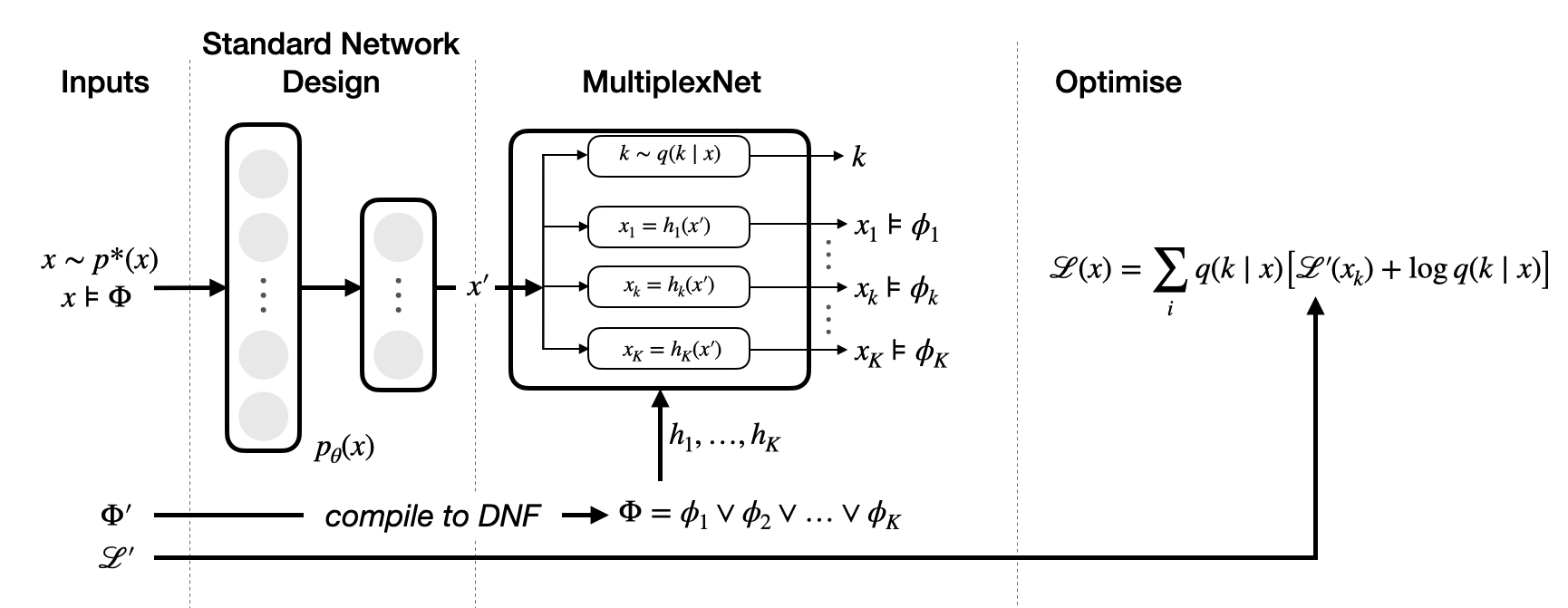
This paper directly addresses these challenges by providing a new way of representing domain constraints directly in the output layer of a network that guarantees constraint satisfaction. The proposed approach represents domain knowledge as a logical formula in disjunctive normal form (DNF). It augments the output layer of an existing neural network to include a separate transformation for each term in the DNF formula. We introduce a latent Categorical variable that selects the best transformation that optimizes the loss function of the data. In this way, we are able to represent arbitrarily complex domain constraints in an automated manner, and we are also able to guarantee that the output of the network satisfies the specified constraints.
We show the efficacy of this MultiplexNet approach in three distinct experiments. First, we present a density estimation task on synthetic data. It is a common goal in machine learning to draw samples from a target distribution, and deep generative models have shown to be flexible and powerful tools for solving this problem. We show that by including domain knowledge, a model can learn to approximate an unknown distribution on fewer samples, and the model will (by construction) only produce samples that satisfy the domain constraints. This experiment speaks to both the data efficiency and the guaranteed constraint satisfaction desiderata. Second, we present an experiment on the popular MNIST data set (LeCun, Cortes, and Burges 2010) which combines structured data with domain knowledge. We structure the digits in a similar manner to the MNIST experiment from Manhaeve et al. (2018); however, we train the network in an entirely label-free manner (Stewart and Ermon 2017). In our third experiment, we apply our approach to the well known image classification task on the CIFAR100 data set (Krizhevsky, Hinton et al. 2009). Images are clustered according to “super classes” (e.g., both maple tree and oak tree fall under the super class tree). We follow the example of Fischer et al. (2019) and show that by including the knowledge that images within a super class are related, we can increase the classification accuracy at the super class level.
The paper contributes a novel and general way to integrate domain knowledge in the form of a logical specification into the training of neural networks. We show that domain knowledge may be used to restrict the network’s operating domain such that any output is guaranteed to satisfy the constraints; and in certain cases, the domain knowledge can help to train the networks on fewer samples of data.
Problem Specification
We consider a data set of i.i.d. samples from a hybrid (some mixture of discrete and/or continuous variables) probability density (Belle, Passerini, and Van den Broeck 2015). Moreover, we assume that: (1) the data set was generated by some random process ; and (2) there exists domain or expert knowledge, in the form of a logical formula , about the random process that can express the domain where is feasible (non-zero). Both of these assumptions are summarised in Eq. 1. In Eq. 1, the notation , denotes that the sample satisfies the formula (Barrett et al. 2009). For example, if , and given some sample , we denote: .
| (1) |
Our aim is to approximate with some parametric model and to incorporate the domain knowledge into the maximum likelihood estimation of , on the available data set.
Given knowledge of the constraints , we are interested in ways of integrating these constraints into the training of a network that approximates . We desire an algorithm that does not require novel engineering to solve a reparameterisation of the network and moreover, especially salient for safety-critical domains, any sample from the model, , should imply that the constraints are satisfied. This is an especially important aspect to consider when comparing this method to alternative approaches, namely Fischer et al. (2019) and Xu et al. (2018), that do not give this same guarantee.
Related Work
The integration of domain knowledge into the training of neural networks is an emerging area of focus. Many previous studies attempt to translate logical constraints into a numerical loss. The two most relevant works in this line are the DL2 framework by Fischer et al. (2019) and the Semantic Loss approach by Xu et al. (2018). DL2 uses a loss term that trades off data with the domain knowledge. It defines a non-negative loss by interpreting the logical constraints using fuzzy logic and defining a measure that quantifies how far a network’s output is from the nearest satisfying solution. Semantic Loss also defines a term that is added to the standard network loss. Their loss function uses weighted model counting (Chavira and Darwiche 2008) to evaluate the probability that a sample from a network’s output satisfies some Boolean constraint formulation. We differ from both of these approaches in that we do not add a loss term to the network’s loss function, rather we compile the constraints directly into its output. Furthermore, in contrast to the works above, any network output from MultiplexNet will satisfy the domain constraints, which is crucial in safety critical domains.
It is also important to compare the expressiveness of the MultiplexNet constraints to those permitted by Fischer et al. (2019) and Xu et al. (2018). In MultiplexNet, the constraints can consist of any quantifier-free linear arithmetic formula over the rationals. Thus, variables can be combined over and , and formulae over , and . For example, but also are well defined formulae and therefore well defined constraints in our framework. The expressiveness is significant — for example, Xu et al. (2018) only allow for Boolean variables over . While Fischer et al. (2019) allow non-Boolean variables to be combined over and formulae to be used over , it is not a probabilistic framework, but one that is based on fuzzy logic. Thus, our work is probabilistic like the Semantic Loss (Xu et al. 2018), but it is more expressive in that it also allows real-valued variables over summations too.
Hu et al. (2016) introduce “iterative rule knowledge distillation” which uses a student and teacher framework to balance constraint satisfaction on first order logic formulae with predictive accuracy on a classification task. During training, the student is used to form a constrained teacher by projecting its weights onto a subspace that ensures satisfaction of the logic. The student is then trained to imitate the teacher’s restricted predictions. Hu et al. (2016) use soft logic (Bach et al. 2017) to encode the logic, thereby allowing gradient estimation; however, the approach is unable to express rules that constrain real-valued outputs. Xsat (Fu and Su 2016) focuses on the Satisfiability Modulo Theory (SMT) problem, which is concerned with deciding whether a (usually a quantifier-free form) formula in first-order logic is satisfied against a background arithmetic theory; similar to what we consider. They present a means for solving SMT formulae but this is not differentiable. Manhaeve et al. (2018) present a compelling method for integrating logical constraints, in the form of a ProbLog program, into the training of a network. However, the networks are embedded into the logic (represented by a Sentential Decision Diagram (Darwiche 2011)), as “neural predicates” and thus it is not clear how to handle the real-valued arithmetic constraints that we represent in MultiplexNet.
We also relate to work on program synthesis (Solar-Lezama 2009; Jha et al. 2010; Feng et al. 2017; Osera 2019) where the goal is to produce a valid program for a given set of constraints. Here, the output of a program is designed to meet a given specification. These works differ from this paper as they don’t focus on the core problem of aiding training with the constraints and ensuring that the constraints are fully satisfied.
Other recent works have also explored how human expert knowledge can be used to guide a network’s training. Ross and Doshi-Velez (2018); Ross, Hughes, and Doshi-Velez (2017) explore how the robustness of an image classifier can be improved by regularizing input gradients towards regions of the image that contain information (as identified by a human expert). They highlight the difficulty in eliciting expert knowledge from people but their technique is similar to the other works presented here in that the knowledge loss is still represented as an additive term to the standard network loss. Takeishi and Kawahara (2020) present an example of how the knowledge of relations of objects can be used to regularise a generative model. Again, the solution involves appending terms to the loss function, but they demonstrate that relational information can aid a learning algorithm. Alternative works have also explored means for constraining the latent variables in a latent variable model (Ganchev et al. 2010; Graça, Ganchev, and Taskar 2007). In contrast to this, we focus on constraining the output space of a generative model, rather than the latent space.
Finally, we mention work on the post-hoc verification of networks. Examples include the works of Katz et al. (2017) and Bunel et al. (2018) who present methods for validating whether a network will operate within the bounds of pre-defined restrictions. Our own work focuses on how to guarantee that the networks operate within given constraints, rather than how to validate their output.
Incorporating Domain Constraints into Model Design
We begin by describing how a satisfiability problem can be hard coded into the output of a network. We then present how any specification of knowledge can be compiled into a form that permits this encoding. An overview of the proposed architecture with a general algorithm that details how to incorporate domain constraints into training a network can be found in Appendix B in the supplementary material.
Satisfiability as Reparameterisation
Let denote the unconstrained output of a network. Let be a network activation that is element-wise non-negative (for example an exponential function, or a ReLU (Nair and Hinton 2010) or Softplus (Dugas et al. 2001) layer). If the property to be encoded is a simple inequality , it is sufficient to constrain to be non-negative by applying and thereafter applying a linear transformation such that: . In this case, can implement the transformation where is the operator that returns the sign of . By construction we have:
| (2) |
It follows that more complex conjunctions of constraints can be encoded by composing transformations of the form presented in Eq. 2. We present below a few examples to demonstrate how this can be achieved for a number of common constraints (where always refers to the unconstrained output of the network):
| (3) | ||||
| (4) | ||||
| (5) |
In Eq 3, we introduce the function . This is merely a function to compute the correct offset for a given activation . In the case of the Softplus function, which is the function used in all of our experiments, .
In Section: Experiments, we implement three varied experiments that demonstrate how complex constraints can be constructed from this basic primitive in Eq. 2. Conceptually, appending additional conjunctions to serves to restrict the space that the output can represent. However, in many situations domain knowledge will consist of complicated formulae that exist well beyond mere conjunctions of inequalities.
While conjunctions serve to restrict the space permitted by the network’s output, disjunctions serve to increase the permissible space. For two terms and in there exist three possibilities: namely, that or or . Given the fact that any unconstrained network output can be transformed to satisfy some term , we propose to introduce multiple transformations of a network’s unconstrained output, each to model the different terms . In this sense, the network’s output layer can be viewed as a multiplexor in a logical circuit that permits for a branching of logic. If represents the transformation of that satisfies and then we know the output must also satisfy by choosing either or . It is this branching technique for dealing with disjunctions that gives rise to the name of the approach: MultiplexNet.
We finally turn to the desideratum of allowing any Boolean formula over linear inequalities as the input for the domain constraints. The suggested approach can represent conjunctions of constraints and disjunctions between these conjunctive terms, which is exactly a DNF representation. Thus, the approach can be used with any transformed version of that is in DNF (Darwiche and Marquis 2002). We propose to use an off-the-shelf solver, e.g., Z3 (De Moura and Bjørner 2008), to provide the logical input to the algorithm that is in DNF. We thus assume the domain knowledge is expressed as:
| (6) |
If is the branch of MultiplexNet that ensures the output of the network then it follows by construction that for all . For example, consider a network with a single real-valued output . If the knowledge , we would then have the two terms and . Here, is the network activation that is element-wise non-negative that was referred to in Section: Satisfiability as Reparameterisation. It is clear that both and satisfy the formula .
Lemma 0.1
Suppose is a quantifier free first-order formula in DNF over consisting of terms . Since each branch of MultiplexNet () is constructed to satisfy a specific term (), by construction, the output of MultiplexNet will satisfy : .
MultiplexNet as a Latent Variable Problem
MultiplexNet introduces a latent Categorical variable that selects among the different terms . The model then incorporates a constraint transformation term conditional on the value of the Categorical variable.
| (7) |
A lower bound on the likelihood of the data can be obtained by introducing a variational approximation to the latent Categorical variable . This standard form of the variational lower bound (ELBO) is presented in Eq. 8.
| (8) |
Gradient based methods require calculating the derivative of Eq. 8. However, as is a Categorical distribution, the standard reparameterisation trick cannot be applied (Kingma and Welling 2014). One possibility for dealing with this expectation is to use the score function estimator, as in REINFORCE (Williams 1992); however, while the resulting estimator is unbiased, it has a high variance (Mnih and Gregor 2014). It is also possible to replace the Categorical variable with a continuous approximation as is done by Maddison, Mnih, and Teh (2017) and Jang, Gu, and Poole (2016); or, if the dimensionality of the Categorical variable is small, it can be marginalised out as in (Kingma et al. 2014). In the experiments in Section: Experiments, we follow Kingma et al. (2014) and marginalise this variable,222Although we note that the alternatives should also be explored. leading to the following learning objective:
| (9) |
We show in Section: Experiments that this approach can be applied equally successfully for a generative modeling task (where the goal is density estimation) as for a discriminative task (where the goal is structured classification). This helps to demonstrate the universal applicability of incorporating domain knowledge into the training of networks.
Experiments
We apply MultiplexNet to three separate experimental domains. The first domain demonstrates a density estimation task on synthetic data when the number of available data samples are limited. We show how the value of the domain constraints improves the training when the number of data samples decreases; this demonstrates the power of adding domain knowledge into the training pipeline. The second domain applies MultiplexNet to labeling MNIST images in an unsupervised manner by exploiting a structured problem and data set. We use a similar experimental setup to the MNIST experiment from DeepProbLog (Manhaeve et al. 2018); however, we present a natural integration with a generative model that is not possible with DeepProbLog. The third experiment uses hierarchical domain knowledge to facilitate an image classification task taken from Fischer et al. (2019) and Xu et al. (2018). We show how the use of this knowledge can help to improve classification accuracy at the super class level.
Synthetic Data
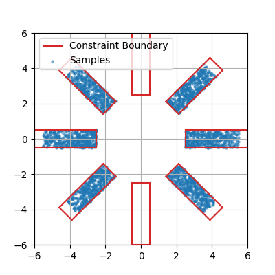
In this illustrative experiment, we consider a target data set that consists of the six rectangular modes that are shown in Figure 1. The samples from the true target density are shown, along with rectangular boxes in red. The rectangular boxes represent the domain constraints for this experiment. Here, we show that an expert might know where the data can exist but that the domain knowledge does not capture all of the details of the target density. Thus, the network is still tasked with learning the intricacies of the data that the domain constraints fail to address (e.g., not all of the area within the constraints contains data). However, we desire that the knowledge leads the network towards a better solution, and also to achieve this on fewer data samples from the true distribution.
This experiment represents a density estimation task and thus we use a likelihood-based generative model to represent the unknown target density, using both data samples and domain knowledge. We use a variational autoencoder (VAE) which optimizes a lower bound to the marginal log-likelihood of the data. However, a different generative model, for example a normalizing flow (Papamakarios et al. 2019) or a GAN (Goodfellow et al. 2014), could as easily be used in this framework. We optimize Eq. 9 where, for this experiment, the likelihood term is replaced by the standard VAE loss. Additional experimental details, as well as the full loss function, can be found in Appendix A.
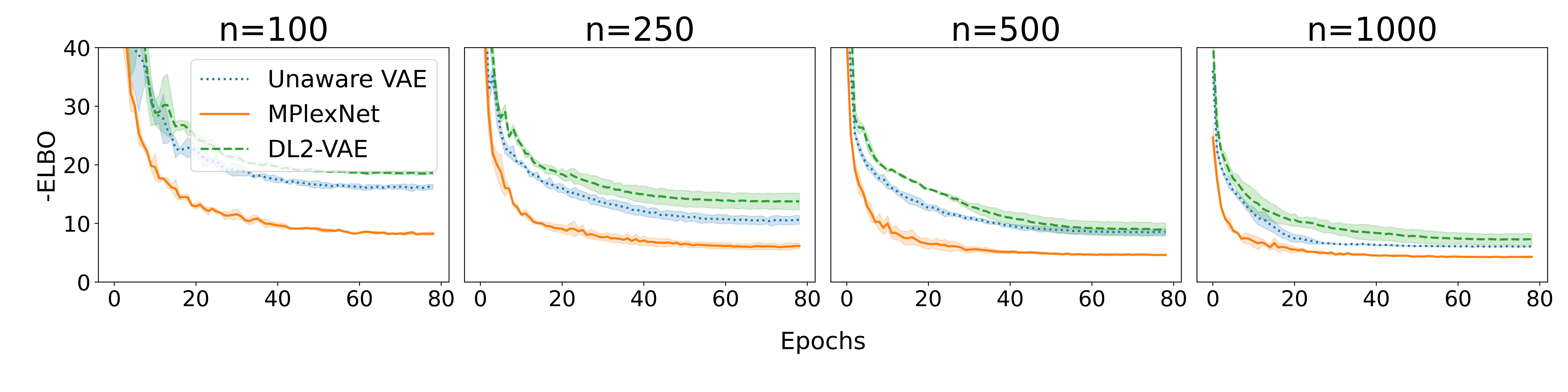
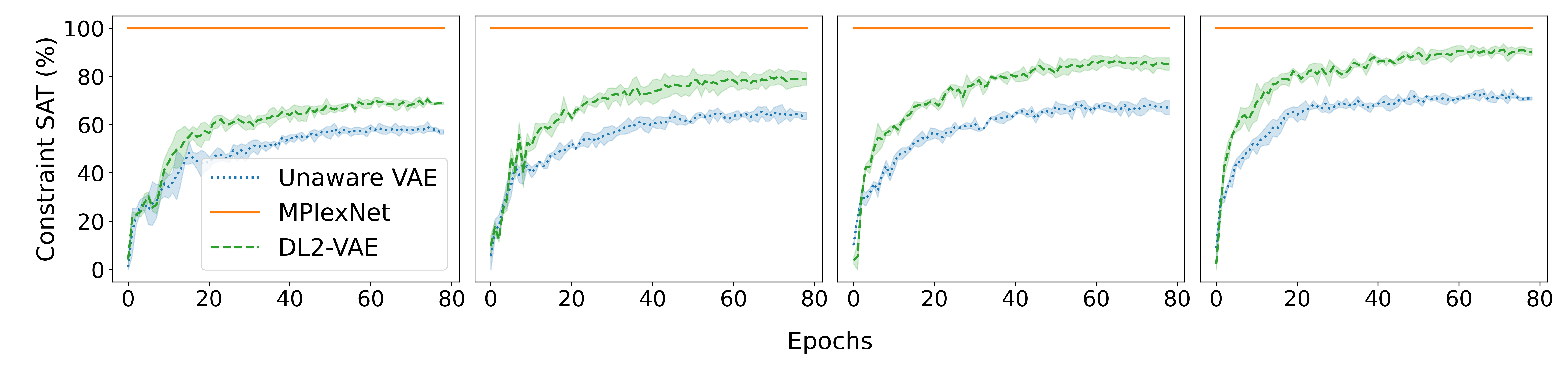
We vary the size of the training data set with as the four experimental conditions. We compare the lower bound to the marginal log-likelihood under three conditions: the MultiplexNet approach, as well as two baselines. The first baseline (Unaware VAE) is a vanilla VAE that is unaware of the domain constraints. This scenario represents the standard setting where domain knowledge is simply ignored in the training of a deep generative network. The second baseline (DL2-VAE) represents a method that appends a loss term to the standard VAE loss. It is important to note that this approach, from DL2 (Fischer et al. 2019), does not guarantee that the constraints are satisfied (clearly seen in Figure 2(b)).
Figure 2 presents the results where we run the experiment on the specified range of training data set sizes. The top plot shows the variational loss as a function of the number of epochs. For all sizes of training data, the MultiplexNet loss on a test set can be seen to outperform the baselines. By including domain knowledge, we can reach a better result, and on fewer samples of data, than by not including the constraints. More important than the likelihood on held-out data is that the samples from the models’ posterior should conform with the constraints. Figure 2(b) shows that the baselines struggle to learn the structure of the constraints. While the MultiplexNet solution is unsurprising, the constraints are followed by construction, the comparison to the baselines is stark. We also present samples from both the prior and the posterior for all of these models in Appendix A. In all of these, MultiplexNet learns to approximate the unknown density within the predefined boundaries of the provided constraints.
MNIST - Label-free Structured Learning
We demonstrate how a structured data set, in combination with the relevant domain knowledge, can be used to make novel inferences in that domain. Here, we use a similar experiment to that from Kingma et al. (2014) where we model the MNIST digit data set in an unsupervised manner. Moreover, we take inspiration from Manhaeve et al. (2018) for constructing a structured data set were the images represent the terms in a summation (e.g., ). However, we add to the complexity of the task by (1) using no labels for any of the images;333In the MNIST experiment from Manhaeve et al. (2018), the authors use the result of the summation as labels for the algorithm. We have no such analogy in this experiment and thus cannot use their DeepProbLog implementation as a baseline. and, (2) considering a generative task.
Kingma et al. (2014) propose a generative model that reasons about the cluster assignment of a data point (a single image). In particular, in their popular “Model 2,” they describe a generative model for an image such that the probability of the image pixel values are conditioned on a latent variable () and a class label (): . We can interpret this model using the MultiplexNet framework where the cluster assignment label implies that the image was generated from cluster . Given a reconstruction loss for image , conditioned on class label (), the domain knowledge in this setting is: . We can successfully model the clustering of the data using this setup but there is no means for determining which label corresponds to which cluster assignment.
We therefore propose to augment the data set such that each input is a quintuple of four images in the form . Here, the inputs and can be any integer from to and the result is a two digit number from to . While we do not know explicitly any of the cluster labels, we do know that the data conform to this standard. Thus for all where , the domain knowledge is of the form:
| (10) |
In this setting, the categorical variable in the MultiplexNet chooses among the combinations that satisfy . This experiment has similarities to DeepProbLog (Manhaeve et al. 2018) as the primitive is repeated for each digit. In this sense, it is similar to the “neural predicate” used by Manhaeve et al. (2018), and the MultiplexNet output layer implements what would be the logical program from DeepProbLog. However, it is not clear how to implement this label-free, generative task within the DeepProbLog framework.
In Figure 3, we present samples from the prior, conditioned on the different class labels. The model is able to learn a class-conditional representation for the data, given no labels for the images. This is in contrast to a vanilla model (from Kingma et al. (2014)) which does not use the structure of the data set to make inferences about the class labels. We present these baseline samples as well as the experimental details and additional notes in Appendix A. Empirically, the results from this experiment were sensitive to the network’s initialisation and thus we report the accuracy of the top runs. We selected the runs based on the loss (the ELBO) on a validation set (i.e., the labels were still not used in selecting the run). The accuracy of the inferred labels on held out data is .
Hierarchical Domain Knowledge on CIFAR100
| Model | Class Accuracy | Super-class Accuracy | Constraint Satisfaction |
|---|---|---|---|
| Vanilla ResNet | |||
| Vanilla ResNet (SC only) | NA | NA | |
| Hierarchical Model | |||
| DL2 | |||
| MultiplexNet |
The final experiment demonstrates how to encode hierarchical domain knowledge into the output layer of a network. The CIFAR100 (Krizhevsky, Hinton et al. 2009) data set consists of classes of images where the classes are in turn broken into super-classes (SC). We wish to encode the belief that images from the same SC are semantically related. Following the encoding in Fischer et al. (2019), we consider constraints which specify that groups of classes should together be very likely or very unlikely. For example, suppose that the SC label is trees and the class label is maple. Our domain knowledge should state that the trees group must be very likely even if there is uncertainty in the specific label maple. Intuitively, it is egregious to misclassify this example as a tractor but it would be acceptable to make the mistake of oak. This can be implemented by training a network to predict first the SC for an unknown image and thereafter the class label, conditioned on the value for the SC.
We chose rather to implement this same knowledge using the MultiplexNet framework. Let denote the output of a network that predicts the class label within the SC. Let denote the minimum requirement for a SC prediction (e.g., if , we require that a SC be predicted with probability or more). The domain knowledge is:
| (11) |
Eq. 11 states that for all labels within a SC group, the unnormalised logits of the network should be greater than the normalised sum of the other labels belonging to the other SCs with a margin of . We explain Eq. 11 further and present other experimental details in Appendix A. This constraint places a semantic grouping on the data as the network is forced into a low entropy prediction at the super class level.
We compare the performance of MultiplexNet to three baselines and report the prediction accuracy on the fine class label as well that on the super class label. We use a Wide ResNet 28-10 (Zagoruyko and Komodakis 2016) model in all of the experimental conditions. The first two baselines (Vanilla) only use the Wide ResNet model and are trained to predict the fine class and the super class labels respectively. The second baseline (Hierarchical) is trained to predict the super class label and thereafter the fine class label, conditioned on the value for the super class label. This represents the bespoke engineering solution to this hierarchical problem. The final baseline (DL2) implements the same logical specification that is used for MultiplexNet but uses the DL2 framework to append to the standard cross-entropy loss function.
Table 1 presents the results for this experiment. Firstly, it is important to note the difficulty of this task. The Vanilla ResNet that predicts only the super-class labels for the images under performs the baseline that is tasked with predicting the true class label. Moreover, while the hierarchical baseline does outperform the vanilla models on the task of super-class prediction, this comes at a cost to the true class accuracy. As the hierarchical baseline represents the bespoke engineering solution to the problem, it also achieves constraint satisfaction, but this comes at the cost of domain specific and custom implementation. The MultiplexNet approach provides a slight improvement at the SC classification accuracy and importantly, the domain constraints are always met. As the domain knowledge prioritizes the accuracy at the SC level, we note that the MultiplexNet approach does not outperform the Vanilla ResNet at the class accuracy. Surprisingly, the DL2 baseline improves upon the class accuracy but it has a limited impact on the super class accuracy and on the constraint satisfaction.
Limitations and Discussion
The limitations of the suggested approach relate to the technical specification of the domain knowledge and to the practical implementation of this knowledge. We discuss first these two aspects and then we discuss a potential negative societal impact.
First, we require that experts be able to express precisely, in the form of a logical formula, the constraints that are valid for their domain. This may not always be possible. For example, given an image classification task, we may wish to describe our knowledge about the content of the images. Consider an example where images contain pictures of dogs and fish and that we wish to express the knowledge that dogs must have four legs and fish must be in water. It is not clear how these conceptual constraints would then be mapped to a pixel level for actual specification. Moreover, it is entirely plausible to have images of dogs that do not include their legs, or images of fish where the fish is out of the water. The logical statement itself is brittle in these instances and would serve to hinder the training, rather than to help it. This example serves to present the inherent difficulty that is present when actually expressing robust domain knowledge in the form of logical formulae.
The second major limitation of this approach deals with the DNF requirement on the input formula. We require that knowledge be expressed in this form such that the “or” condition is controlled by the latent Categorical variable of MultiplexNet. It is well known that certain formulae have worst case representations in DNF that are exponential in the number of variables. This is clearly undesirable in that the network would have to learn to choose among the exponentially many terms.
One of the overarching motivations for this work is to constrain networks for safety critical domains. While constrained operation might be desired on many accounts, there may exist edge cases where an autonomously acting agent should act in an undesirable manner to avoid an even more undesirable outcome (a thought experiment of this spirit is the well known Trolley Problem (Hammond and Belle 2021)). By guaranteeing that the operating conditions of a system be restricted to some range, our approach does encounter vulnerability with respect to edge, and unforeseen, cases. However, to counter this point, we argue it is still necessary for experts to define the boundaries over the operation domain of a system in order to explicitly test and design for known worst case scenario settings.
Conclusions and Future Work
This work studied how logical knowledge in an expressive language could be used to constrain the output of a network. It provides a new and general way to encode domain knowledge as logical constraints directly in the output layer of a network. Compared to alternative approaches, we go beyond propositional logic by allowing for arithmetic operators in our constraints. We are able to guarantee that the network output is 100% compliant with the domain constraints, which the alternative approaches, which append a “constraint loss,” are unable to match. Thus our approach is especially relevant for safety critical settings in which the network must guarantee to operate within predefined constraints. In a series of experiments we demonstrated that our approach leads to better results in terms of data efficiency (the amount of training data that is required for good performance), reducing the data burden that is placed on the training process. In the future, we are excited about exploring the prospects for using this framework on downstream tasks, such as robustness to adversarial attacks.
References
- Allen, Balažević, and Hospedales (2020) Allen, C.; Balažević, I.; and Hospedales, T. 2020. A Probabilistic Framework for Discriminative and Neuro-Symbolic Semi-Supervised Learning. arXiv preprint arXiv:2006.05896.
- Amodei et al. (2016) Amodei, D.; Olah, C.; Steinhardt, J.; Christiano, P.; Schulman, J.; and Mané, D. 2016. Concrete problems in AI safety. arXiv preprint arXiv:1606.06565.
- Bach et al. (2017) Bach, S. H.; Broecheler, M.; Huang, B.; and Getoor, L. 2017. Hinge-Loss Markov Random Fields and Probabilistic Soft Logic. J. Mach. Learn. Res., 18(1): 3846–3912.
- Barrett et al. (2009) Barrett, C.; Sebastiani, R.; Seshia, S. A.; Tinelli, C.; Biere, A.; Heule, M.; van Maaren, H.; and Walsh, T. 2009. Handbook of satisfiability. Satisfiability modulo theories, 185: 825–885.
- Belle, Passerini, and Van den Broeck (2015) Belle, V.; Passerini, A.; and Van den Broeck, G. 2015. Probabilistic inference in hybrid domains by weighted model integration. In Proceedings of 24th International Joint Conference on Artificial Intelligence (IJCAI), volume 2015, 2770–2776.
- Brown et al. (2020) Brown, T. B.; Mann, B.; Ryder, N.; Subbiah, M.; Kaplan, J.; Dhariwal, P.; Neelakantan, A.; Shyam, P.; Sastry, G.; Askell, A.; et al. 2020. Language models are few-shot learners. arXiv preprint arXiv:2005.14165.
- Bunel et al. (2018) Bunel, R.; Turkaslan, I.; Torr, P. H. S.; Kohli, P.; and Mudigonda, P. K. 2018. A Unified View of Piecewise Linear Neural Network Verification. Advances in Neural Information Processing Systems, 4795–4804.
- Chavira and Darwiche (2008) Chavira, M.; and Darwiche, A. 2008. On probabilistic inference by weighted model counting. Artificial Intelligence, 172(6-7): 772–799.
- Darwiche (2011) Darwiche, A. 2011. SDD: A new canonical representation of propositional knowledge bases. In Twenty-Second International Joint Conference on Artificial Intelligence.
- Darwiche and Marquis (2002) Darwiche, A.; and Marquis, P. 2002. A knowledge compilation map. Journal of Artificial Intelligence Research, 17: 229–264.
- De Moura and Bjørner (2008) De Moura, L.; and Bjørner, N. 2008. Z3: An efficient SMT solver. In International conference on Tools and Algorithms for the Construction and Analysis of Systems, 337–340. Springer.
- Dosovitskiy et al. (2020) Dosovitskiy, A.; Beyer, L.; Kolesnikov, A.; Weissenborn, D.; Zhai, X.; Unterthiner, T.; Dehghani, M.; Minderer, M.; Heigold, G.; Gelly, S.; et al. 2020. An image is worth 16x16 words: Transformers for image recognition at scale. arXiv preprint arXiv:2010.11929.
- Dugas et al. (2001) Dugas, C.; Bengio, Y.; Bélisle, F.; Nadeau, C.; and Garcia, R. 2001. Incorporating second-order functional knowledge for better option pricing. Advances in neural information processing systems, 472–478.
- Feng et al. (2017) Feng, Y.; Martins, R.; Wang, Y.; Dillig, I.; and Reps, T. W. 2017. Component-Based Synthesis for Complex APIs. In Proceedings of the 44th ACM SIGPLAN Symposium on Principles of Programming Languages, 599–612.
- Fischer et al. (2019) Fischer, M.; Balunovic, M.; Drachsler-Cohen, D.; Gehr, T.; Zhang, C.; and Vechev, M. 2019. DL2: Training and Querying Neural Networks with Logic. In Proceedings of the 36th International Conference on Machine Learning, 1931–1941.
- Fu and Su (2016) Fu, Z.; and Su, Z. 2016. XSat: A Fast Floating-Point Satisfiability Solver. In Proceedings of the 28th International Conference on Computer Aided Verification, Part II, 187–209. Springer. ISBN 978-3-319-41539-0.
- Ganchev et al. (2010) Ganchev, K.; Graça, J.; Gillenwater, J.; and Taskar, B. 2010. Posterior regularization for structured latent variable models. The Journal of Machine Learning Research, 11: 2001–2049.
- Goodfellow et al. (2016) Goodfellow, I.; Bengio, Y.; Courville, A.; and Bengio, Y. 2016. Deep learning, volume 1. MIT press Cambridge.
- Goodfellow et al. (2014) Goodfellow, I.; Pouget-Abadie, J.; Mirza, M.; Xu, B.; Warde-Farley, D.; Ozair, S.; Courville, A.; and Bengio, Y. 2014. Generative adversarial nets. In Advances in neural information processing systems, 2672–2680.
- Graça, Ganchev, and Taskar (2007) Graça, J. V.; Ganchev, K.; and Taskar, B. 2007. Expectation maximization and posterior constraints.
- Hammond and Belle (2021) Hammond, L.; and Belle, V. 2021. Learning tractable probabilistic models for moral responsibility and blame. Data Mining and Knowledge Discovery, 35(2): 621–659.
- Hu et al. (2016) Hu, Z.; Ma, X.; Liu, Z.; Hovy, E.; and Xing, E. 2016. Harnessing Deep Neural Networks with Logic Rules. In Proceedings of the 54th Annual Meeting of the Association for Computational Linguistics (Volume 1: Long Papers), 2410–2420.
- Jang, Gu, and Poole (2016) Jang, E.; Gu, S.; and Poole, B. 2016. Categorical reparameterization with gumbel-softmax. arXiv preprint arXiv:1611.01144.
- Jha et al. (2010) Jha, S.; Gulwani, S.; Seshia, S. A.; and Tiwari, A. 2010. Oracle-Guided Component-Based Program Synthesis. In Proceedings of the 32nd ACM/IEEE International Conference on Software Engineering - Volume 1, 215–224.
- Katz et al. (2017) Katz, G.; Barrett, C.; Dill, D. L.; Julian, K.; and Kochenderfer, M. J. 2017. Reluplex: An efficient SMT solver for verifying deep neural networks. In International Conference on Computer Aided Verification, 97–117. Springer.
- Kingma et al. (2014) Kingma, D. P.; Mohamed, S.; Rezende, D. J.; and Welling, M. 2014. Semi-supervised learning with deep generative models. In Advances in neural information processing systems, 3581–3589.
- Kingma and Welling (2014) Kingma, D. P.; and Welling, M. 2014. Auto-encoding variational bayes. In 2nd International Conference on Learning Representations (ICLR).
- Krizhevsky, Hinton et al. (2009) Krizhevsky, A.; Hinton, G.; et al. 2009. Learning multiple layers of features from tiny images.
- LeCun, Cortes, and Burges (2010) LeCun, Y.; Cortes, C.; and Burges, C. 2010. MNIST handwritten digit database. ATT Labs [Online]. Available: http://yann.lecun.com/exdb/mnist, 2.
- Maddison, Mnih, and Teh (2017) Maddison, C. J.; Mnih, A.; and Teh, Y. W. 2017. The concrete distribution: A continuous relaxation of discrete random variables. In 5th International Conference on Learning Representations (ICLR).
- Manhaeve et al. (2018) Manhaeve, R.; Dumancic, S.; Kimmig, A.; Demeester, T.; and De Raedt, L. 2018. Deepproblog: Neural probabilistic logic programming. Advances in Neural Information Processing Systems, 31: 3749–3759.
- Mnih and Gregor (2014) Mnih, A.; and Gregor, K. 2014. Neural variational inference and learning in belief networks. In International Conference on Machine Learning, 1791–1799. PMLR.
- Nair and Hinton (2010) Nair, V.; and Hinton, G. E. 2010. Rectified Linear Units Improve Restricted Boltzmann Machines. In Proceedings of the 27th International Conference on International Conference on Machine Learning, ICML’10, 807–814.
- Osera (2019) Osera, P.-M. 2019. Constraint-Based Type-Directed Program Synthesis. In Proceedings of the 4th ACM SIGPLAN International Workshop on Type-Driven Development, 64–76.
- Papamakarios et al. (2019) Papamakarios, G.; Nalisnick, E.; Rezende, D. J.; Mohamed, S.; and Lakshminarayanan, B. 2019. Normalizing Flows for Probabilistic Modeling and Inference. arXiv preprint arXiv:1912.02762.
- Ross and Doshi-Velez (2018) Ross, A.; and Doshi-Velez, F. 2018. Improving the adversarial robustness and interpretability of deep neural networks by regularizing their input gradients. In Proceedings of the AAAI Conference on Artificial Intelligence, volume 32.
- Ross, Hughes, and Doshi-Velez (2017) Ross, A. S.; Hughes, M. C.; and Doshi-Velez, F. 2017. Right for the Right Reasons: Training Differentiable Models by Constraining their Explanations. In Proceedings of the Twenty-Sixth International Joint Conference on Artificial Intelligence, IJCAI, 2662–2670.
- Solar-Lezama (2009) Solar-Lezama, A. 2009. The Sketching Approach to Program Synthesis. In Proceedings of the 7th Asian Symposium on Programming Languages and Systems, 4–13.
- Stewart and Ermon (2017) Stewart, R.; and Ermon, S. 2017. Label-free supervision of neural networks with physics and domain knowledge. In Proceedings of the AAAI Conference on Artificial Intelligence, volume 31.
- Takeishi and Kawahara (2020) Takeishi, N.; and Kawahara, Y. 2020. Knowledge-Based Regularization in Generative Modeling. In Proceedings of the Twenty-Ninth International Joint Conference on Artificial Intelligence, IJCAI, 2390–2396.
- Williams (1992) Williams, R. J. 1992. Simple statistical gradient-following algorithms for connectionist reinforcement learning. Machine learning, 8(3-4): 229–256.
- Xu et al. (2018) Xu, J.; Zhang, Z.; Friedman, T.; Liang, Y.; and Van den Broeck, G. 2018. A Semantic Loss Function for Deep Learning with Symbolic Knowledge. In Proceedings of the 35th International Conference on Machine Learning, 5502–5511.
- Zagoruyko and Komodakis (2016) Zagoruyko, S.; and Komodakis, N. 2016. Wide Residual Networks. In British Machine Vision Conference.
Appendix A Appendix A: Additional Experimental Details
All code and data for repeating the experiments can be found at the repository at: https://github.com/NickHoernle/semantic_loss. The image experiments (on MNIST and CIFAR100) were run on Nvidia GeForce RTX 2080 Ti devices and the synthetic data experiment was run on a 2015 MacBook Pro with processor specs: 2.2 GHz Quad-Core Intel Core i7. The MNIST data set is available under the Creative Commons Attribution-Share Alike 3.0 license; and CIFAR100 is available under the Creative Commons Attribution-Share Alike 4.0 license. The DL2 framework (available under an MIT License), used in the baselines, is available from https://github.com/eth-sri/dl2.
In all experiments, the data were split into a train, validation and test set where the test set was held constant across the experimental conditions (e.g., in the CIFAR100 experiment, the same test set was used to compare MultiplexNet vs the vanilla models vs the DL2 model). In cases where model selection was performed (early stopping on CIFAR100 and selection of the best runs from the MNIST experiment, we used the validation set to choose the best runs and/or models). In these cases the validation set was extracted from the training data set prior to training (with of the data used for validation). The standard test sets, given by MNIST and CIFAR100 were used for those experiments and an additional test set was generated for the synthetic experiment.
Synthetic Data
Deriving the Loss
We first present the full derivation of the loss function that was used for this experiment. We used a variational autoencoder (VAE) with a standard isotropic Gaussian prior. The standard VAE loss is presented in Eq. 12. In the below formulation, is a datapoint, is a minibatch size, and is a sample from the approximate posterior .
| (12) |
We use an isotropic Gaussian likelihood for and an isotropic Gaussian for the posterior. Standard derivations (see Kingma and Welling (2014) for more details) allow the loss to be expressed as in Eq.13. In this equation, is the decoder model and it predicts the mean of the likelihood term. A tunable parameter controls the precision of the reconstructions – this parameter was held constant for all experimental conditions. The posterior distribution is a Gaussian with parameters and that are output from the encoding network .
| (13) |
Finally, we present how the MultiplexNet loss uses in the transformation of the output layer of the network. MultiplexNet takes as input the unconstrained network output and it outputs the transformed (constrained) terms (for terms in the DNF constraint formulation) and the probability of each term . Let denote the same loss from Eq. 13 but with the raw output of the network constrained by the constraint transformation (i.e., the likelihood term becomes: ) The final loss then is presented in Eq. 14.
| (14) |
Samples from the Posterior
Fig. 4 shows samples from the posterior of the two models – these are the attempts of the VAE to reconstruct the input data. It can clearly be seen that while MultiplexNet strictly adheres to the constraints, the baseline VAE approach fails to capture the constraint boundaries.
Samples from the Prior
Samples from the prior (Fig. 5) show how well a generative model has learnt the data manifold that it attempts to represent. We show these to demonstrate that in this case, the vanilla VAE fails to capture many of the complexities in the data distribution. To sample from the prior for MultiplexNet, we randomly sample from the latent Categorical variable from MultiplexNet. Hence, the two vertical modes (that contain no data in reality) have samples here. This can easily be solved by introducing a trainable prior parameter over the Categorical variable as well – an easy extension that we do not implement in this work.
Network Architecture
The default network used in these experiments was a feed-forward network with a single hidden layer for both the decoder and the encoder models. The dimensionality of the latent random variable was 15 and the hidden layer contained units. ReLU activations were used unless otherwise stated.
MNIST - Label-free Structured Learning
Deriving the Loss
We follow the specification from Kingma et al. (2014) where the likelihood of a single image, , conditioned on a cluster assignment label , is shown in Eq. 15. Again, is a latent parameter, again assumed to follow an isotropic Gaussian distribution.
| (15) |
We refer to the right hand side of Eq. 15 as . Eq. 15 assumes knowledge of the label , but this is unknown for our domain. However, we can implement the knowledge from Eq. 10 (in the main text) that specifies all possibilities for the image inference task. Below we assume the data is of the form where , , and . Finally, we let refer to the MultiplexNet Categorical selection variable that chooses which of the possible terms for are present. Following the MultiplexNet framework, the loss is then presented in Eq 16:
| (16) |
Samples from the Vanilla VAE prior from Kingma et al. (2014)
We repeat the mnist experiment with a vanilla VAE model (“Model 2” from Kingma et al. (2014)). Here we simply show that the model can capture the label clustering of the data but that it cannot, unsurprisingly, infer the class labels correctly from the data without considering the fact that the data set has been structured:
Network Architecture
The default network used in these experiments was a feed-forward network with two hidden layers for both the decoder and the encoder models. The first hidden layer contained units and the second units. The dimensionality of the latent random variable was . ReLU activations were used unless otherwise stated.
Hierarchical Domain Knowledge on CIFAR100
Deriving the Loss
Following the encoding in (Fischer et al. 2019), we consider constraints which specify that groups of classes should together be very likely or very unlikely. For example, suppose that the SC label is trees and the class label is maple. Our domain knowledge should state that the trees group must be very likely even if there is uncertainty in the specific label maple. Fischer et al. (2019) use the following logic to encode this belief (for the super classes that are present in CIFAR100):
| (17) |
This encoding is exactly the same as that presented in Eq 18. However, we re-write this encoding in DNF such that it is compatible with MultiplexNet.
| (18) |
A simplification on the above, as the classes and thus the super classes lie on a simplex, is the specification that necessarily implies that holds too. Thus the logic can again be simplified to:
| (19) |
Again, as the probability values here lie on a simplex, we can represent a single constraint as in Eq 20. Here, is the normalizing constant that ensures the final output values are a valid probability distribution over the class labels (computed with a softmax layer in practice). for all class labels in CIFAR100.
| (20) |
Finally, we can simplify the right hand side of Eq 20 to obtain the following specification (for the super class, but the other SCs all follow via symmetry):
| (21) |
Note that the right hand side of Eq 21 contains the classes for all the other super classes but not including . It thus contains labels in this example.
Studying each of the terms in separately, and noting that is strictly positive, we obtain Eq 22. We use to denote a class label in the target super class (in this case ) and to refer to all other labels in all other super classes (SC).
| (22) |
As we are interested in constraining the unnormalized output of the network () in MultiplexNet, it is clear that we can take the logarithm of both sides of Eq 22 to obtain the final objective for one class label. Together with Eq 19, we then obtain the final logical constraint in the main text in Eq 11.
| (23) |
This implementation can then be directly encoded into the MultiplexNet loss as usual (where refer to the constrained output of the network for each of the super classes, is the MultiplexNet probability for selecting logic term , and is the standard cross entropy loss that is used in image classification.
| (24) |
Network Architecture
We use a Wide ResNet 28-10 (Zagoruyko and Komodakis 2016) in all of the experimental conditions for this CIFAR100 experiment. We build on top of the pytorch implementation of the Wide ResNet that is available here: https://github.com/xternalz/WideResNet-pytorch. This implementation is available under an MIT License.
Appendix B Appendix B: MultiplexNet Architecture Overview
MultiplexNet accepts as input a data set consisting of samples from some target distribution, , and some constraints, that are known about the data set. We assume that the constraints are correct, in that Eq. 1 (main text) holds for all . We aim to model the unknown density, , by maximising the likelihood of a parameterised model, on the given data set. Moreover, our goal is to incorporate the domain constraints, , into the training of this model.
We first assume that the domain constraints are provided in DNF. This is a reasonable assumption as any logical formula can be compiled to DNF, although there might be an exponential number of terms in worst case scenarios (as discussed in Section: Limitations). For each term in the DNF representation of , we then introduce a transformation, , that ensures any real-valued input is transformed to satisfy that term. Given a Softplus transformation , we can suitably restrict the domain of any real-valued variable such that the output satisfies . For example, consider the constraint, e.g., . The transformation will constrain the real-valued variable such that is satisfied. In this example, does not need to be constrained. Here and . Any combination of inequalities can be suitably restricted in this way. Equality constraints, can be handled by simply setting the output to the value that is specified.
MultiplexNet therefore accepts the unconstrained output of a network, , and introduces constraint terms that each guarantee the constrained output will satisfy a term, , in the DNF representation of the constraints. The output of the network is then transformed versions of where each output is guaranteed to satisfy . The Categorical selection variable can be marginalised out leading to the following objective:
| (25) |
In Eq. 25, refers to the observation likelihood that would be used in the absence of any constraint. is the constrained term of the unconstrained output of the network: . This architecture is represented pictorially in Fig. 7.