Evaluating deep transfer learning for
whole-brain cognitive decoding
Abstract
Research in many fields has shown that transfer learning (TL) is well-suited to improve the performance of deep learning (DL) models in datasets with small numbers of samples. This empirical success has triggered interest in the application of TL to cognitive decoding analyses with functional neuroimaging data. Here, we systematically evaluate TL for the application of DL models to the decoding of cognitive states (e.g., viewing images of faces or houses) from whole-brain functional Magnetic Resonance Imaging (fMRI) data. We first pre-train two DL architectures on a large, public fMRI dataset and subsequently evaluate their performance in an independent experimental task and a fully independent dataset. The pre-trained models consistently achieve higher decoding accuracies and generally require less training time and data than model variants that were not pre-trained, clearly underlining the benefits of pre-training. We demonstrate that these benefits arise from the ability of the pre-trained models to reuse many of their learned features when training with new data, providing deeper insights into the mechanisms giving rise to the benefits of pre-training. Yet, we also surface nuanced challenges for whole-brain cognitive decoding with DL models when interpreting the decoding decisions of the pre-trained models, as these have learned to utilize the fMRI data in unforeseen and counterintuitive ways to identify individual cognitive states.
Keywords: cognitive decoding, neuroimaging, deep learning, transfer learning, explainable artificial intelligence
1 Introduction
One of the key challenges for the analysis of functional Magnetic Resonance Imaging (fMRI) data is the high dimensionality and low sample size of conventional fMRI datasets. These datasets typically contain several hundred thousand dimensions (or voxels) for each fMRI volume, while containing only up to a few hundred volumes for each of up to a hundred individuals. To prevent overfitting in these high-dimensional and low-sample size settings, allowing for generalizable statistical inference, conventional approaches for the analysis of fMRI data often include restricting assumptions, by analyzing the data of individual voxels or groups of voxels independent of one another, using simple linear mappings between the cognitive states and brain activity, or by solely focusing on the group level (e.g., Friston et al.,, 1994, Kriegeskorte et al.,, 2006). While these restrictions are well justified for many research questions (e.g., to test whether a specific region-of-interest exhibits more activity in one experimental condition than in another), they also limit the ability of these approaches to capture the temporal and spatial variability of the mapping between a cognitive state (e.g., deciding whether to accept or reject a risky gamble) and the underlying whole-brain brain activity within and between individuals.
Research in many other fields has shown that deep learning (DL; LeCun et al.,, 2015, Goodfellow et al.,, 2016, Schmidhuber,, 2015) methods are generally well-suited to capture complex nonlinear mappings between a target signal (e.g., a cognitive state) and highly variable patterns in the data. For this reason, researchers have started exploring their application to cognitive decoding (e.g., Thomas et al., 2019a, , Abrol et al.,, 2021, Wang et al.,, 2020, Zhang et al.,, 2021, Riaz et al.,, 2020, Suk et al.,, 2016, Schirrmeister et al.,, 2017, Mahmood et al.,, 2020), by training these models to identify (or decode) a set of cognitive states from fMRI data. To subsequently identify an association between the decoded cognitive states and measured brain activity, researchers have turned towards research on explainable artificial intelligence (XAI; Samek et al.,, 2021, Montavon et al.,, 2018, Samek et al., 2017b, ). First empirical work has demonstrated that this combination of DL and XAI is well-suited for the analysis of fMRI data, by accurately decoding cognitive states and identifying biologically plausible associations between the decoded cognitive states and brain activity through the interpretation of a model’s decoding decisions (Thomas et al., 2019a, , Zhang et al.,, 2021, McClure et al.,, 2020, Koyamada et al.,, 2015, Dinsdale et al.,, 2021, Nguyen et al.,, 2020). Yet, many of these studies have also demonstrated that the advantages of DL methods over conventional approaches for the analysis of fMRI data are generally limited to sufficiently large training datasets (Thomas et al., 2019a, , Abrol et al.,, 2021, Schulz et al.,, 2020).
The problem of limited data is not new to the field of machine learning (ML), where researchers have discovered that transfer learning can generally improve the performance of DL models in small datasets. The goal of transfer learning is to leverage the knowledge about the mapping between input data and a target signal that can be learned from one dataset to subsequently improve the learning of a similar mapping in another dataset of a related domain. Transfer learning has been particularly successful in computer vision and natural language processing, where large, publicly available datasets exist (Deng et al.,, 2009, Bowman et al.,, 2015, Rajaraman et al.,, 2018). These datasets are used to first pre-train DL models (e.g., to identify the objects in an image), before fine-tuning them on smaller datasets of a related domain (e.g., to detect breast cancer in medical imaging; Khan et al.,, 2019). When compared to models that are trained from scratch, pre-trained models generally exhibit faster learning and achieve higher predictive accuracies, while also requiring less training data (Yosinski et al.,, 2014, Raffel et al.,, 2020, Kolesnikov et al.,, 2020, Chen et al.,, 2020, Bengio et al.,, 2006, Erhan et al.,, 2010).
Over recent years, neuroimaging research has experienced a strong increase in the availability of public datasets. These datasets are provided by large neuroimaging initiatives (e.g., Van Essen et al.,, 2013, Casey et al.,, 2018, Sudlow et al.,, 2015, Poldrack et al.,, 2016) and individual researchers (e.g., Markiewicz et al.,, 2021). Due to the availability of these datasets, researchers have started exploring whether transfer learning can be beneficial for cognitive decoding analysis with fMRI data. This work generally indicates that the pre-trained models similarly achieve higher decoding accuracies, and require less training time and data, when compared to models that are trained from scratch (Zhang et al.,, 2021, Koyamada et al.,, 2015, Svanera et al.,, 2019, Mahmood et al.,, 2019, Thomas et al., 2019b, , Oh et al.,, 2019, Deepak and Ameer,, 2019, Mensch et al.,, 2021). Yet, this work has often been limited by not evaluating the performance of the pre-trained models in fully independent datasets (e.g., by pre-training on some part of a large dataset and evaluating on another part of the same dataset; Zhang et al.,, 2021, Koyamada et al.,, 2015, Thomas et al., 2019b, ), by using very simple decoding tasks (e.g., by only identifying the dataset or experimental task underlying the fMRI data; Koyamada et al.,, 2015) and experiments (e.g., requiring the experiment to use visual image stimuli; Svanera et al.,, 2019), and by applying strong feature preprocessing to the fMRI data (e.g., independent component, general linear model, and connectivity analyses; Mahmood et al.,, 2019, Mensch et al.,, 2021, Schulz et al.,, 2020, Mahmood et al.,, 2020). Further, many studies have not made their pre-trained DL models available to the public, making it difficult to evaluate the performance of these models in other datasets.
Here, we systematically evaluate deep transfer learning for whole-brain cognitive decoding, by first pre-training two DL architectures on a large whole-brain fMRI dataset and subsequently comparing their performances on an independent experimental task and a fully independent fMRI dataset. We also provide detailed insights into the mechanisms giving rise to the advantages of the pre-trained models, bring forward nuanced challenges for whole-brain cognitive decoding with DL models, and make our pre-trained models available to the public.
Specifically, we train two distinct DL architectures on task-fMRI data from the Human Connectome Project (HCP; Van Essen et al.,, 2013), spanning six experimental tasks and 16 distinct cognitive states. We demonstrate that the pre-trained DL models learn quicker, achieve higher decoding accuracies, and require less training data than model variants that were not pre-trained, when applied to the fMRI data of the left-out seventh HCP experimental task. We further evaluate the performance of the pre-trained models in a fully independent fMRI dataset that is not part of the HCP. Again, the pre-trained models outperform model variants that were not pre-trained by achieving overall higher decoding accuracies and generally learning quicker. To better understand the mechanisms giving rise to the advantages of the pre-trained models, we perform an analysis of their learned hidden representations. This analysis reveals that these advantages generally arise from the ability of the pre-trained models to reuse many of their learned features when training with new data. To also understand the models’ learned mappings between brain activity and cognitive state, we next interpret their cognitive decoding decisions for the fMRI data of the different HCP experimental tasks. We find that the pre-trained models generally associate a similar set of brain regions with the cognitive states of these tasks as a standard general linear model (GLM; Holmes and Friston,, 1998) analysis of the same data. Interestingly, the models identify individual cognitive states by combining activity from brain regions that are generally more active in these states, when compared to other states, with the activity of brain regions that are generally less active in these states. While this represents a biologically plausible solution for the underlying decoding task, the resulting brain maps are, at first sight, surprising, as the models assign high relevance to brain regions that the GLM analysis associates negatively with the decoded cognitive states. Importantly, this pattern only then becomes apparent, when interpreting the models’ decoding decisions in light of the results of the GLM analysis.
In sum, our results highlight that DL models are capable of learning versatile representations of large fMRI datasets, which generalize well to new data and thus allow for successful transfer learning. Yet, these benefits come at a cost, as the underlying learned mappings between brain activity and cognitive states can be complex, unforeseen, and counterintuitive, requiring careful additional analyses to be understood well.
2 Results
2.1 The DeepLight framework
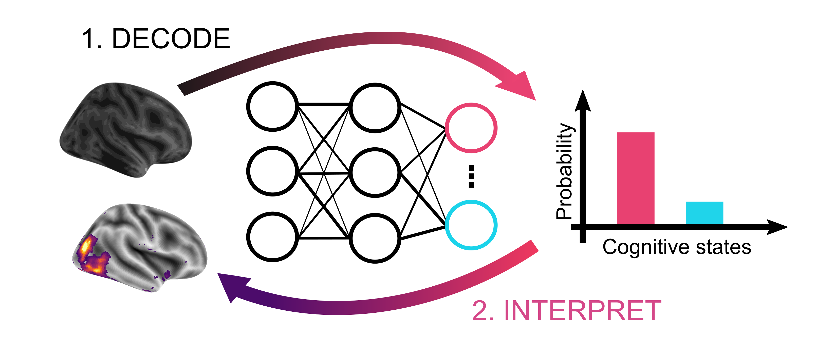
To evaluate the benefits of deep transfer learning for whole-brain cognitive decoding, we utilize the DeepLight framework (Thomas et al., 2019a, , Thomas et al., 2019b, ). DeepLight is defined by two central components (see Fig. 1): It first trains a DL model to decode a set of cognitive states from a single whole-brain fMRI volumes (e.g., single TRs) and subsequently relates the decoded cognitive states and brain activity by interpreting the decoding decisions with methods from XAI. Here, we use the layer-wise relevance propagation (LRP; Bach et al.,, 2015, Montavon et al.,, 2017) technique, which decomposes individual decoding decisions of a DL model into the contributions of the activity of each input voxel to the decisions.
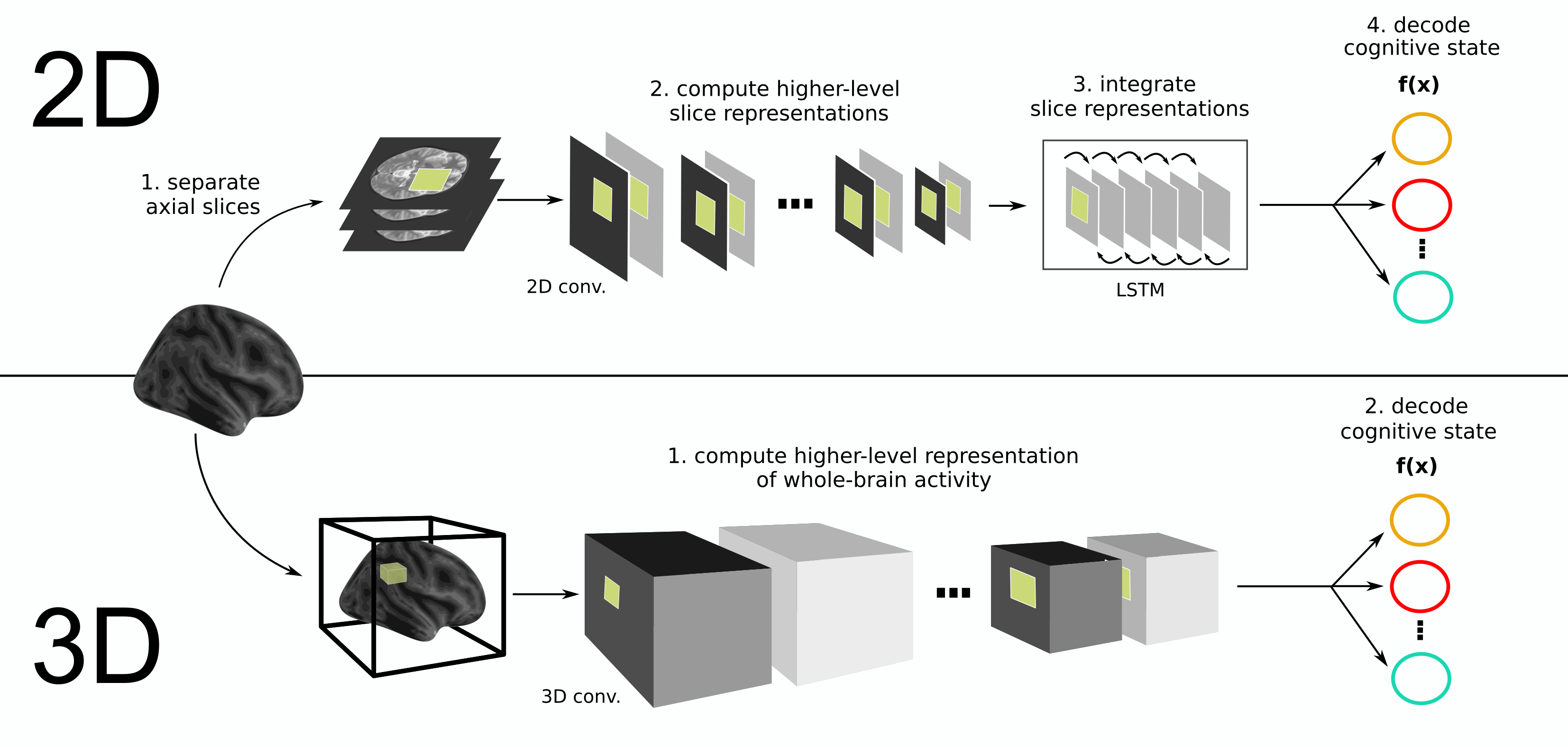
Note that DeepLight is not restricted to any specific DL model architecture. In this work, we explore and compare the performance of two distinct DL model architectures (here abbreviated as ”2D-DeepLight” and ”3D-DeepLight”; see Fig. 2 and section 4.2), which are based on recent empirical work in computer vision (Donahue et al.,, 2017, Marban et al.,, 2019, Tran et al.,, 2015).
2.2 DeepLight accurately decodes cognitive states of the pre-training data
We first pre-trained a variant of each DeepLight architecture (2D and 3D; see Fig. 2 and section 4.2) to identify the cognitive states underlying the individual TRs of a large whole-brain fMRI dataset (for details on the training procedures, see section 4.3), spanning 450 participants in six of the seven HCP experimental tasks (all tasks except for the working memory task; for an overview of the individual experimental tasks, see section 4.1.1 and Appendix A.1). Importantly, all TRs of an experimental block were included in our analyses, except for the first TR of each block, which we excluded.
To evaluate the ability of the 2D- and 3D-DeepLight architectures to identify the cognitive states from individual fMRI volumes (i.e., TRs), we further divided the data within each pre-training task into distinct training and validation datasets, by designating the fMRI data of 400 randomly selected subjects as training data and the data of the remaining 50 subjects as a validation dataset.
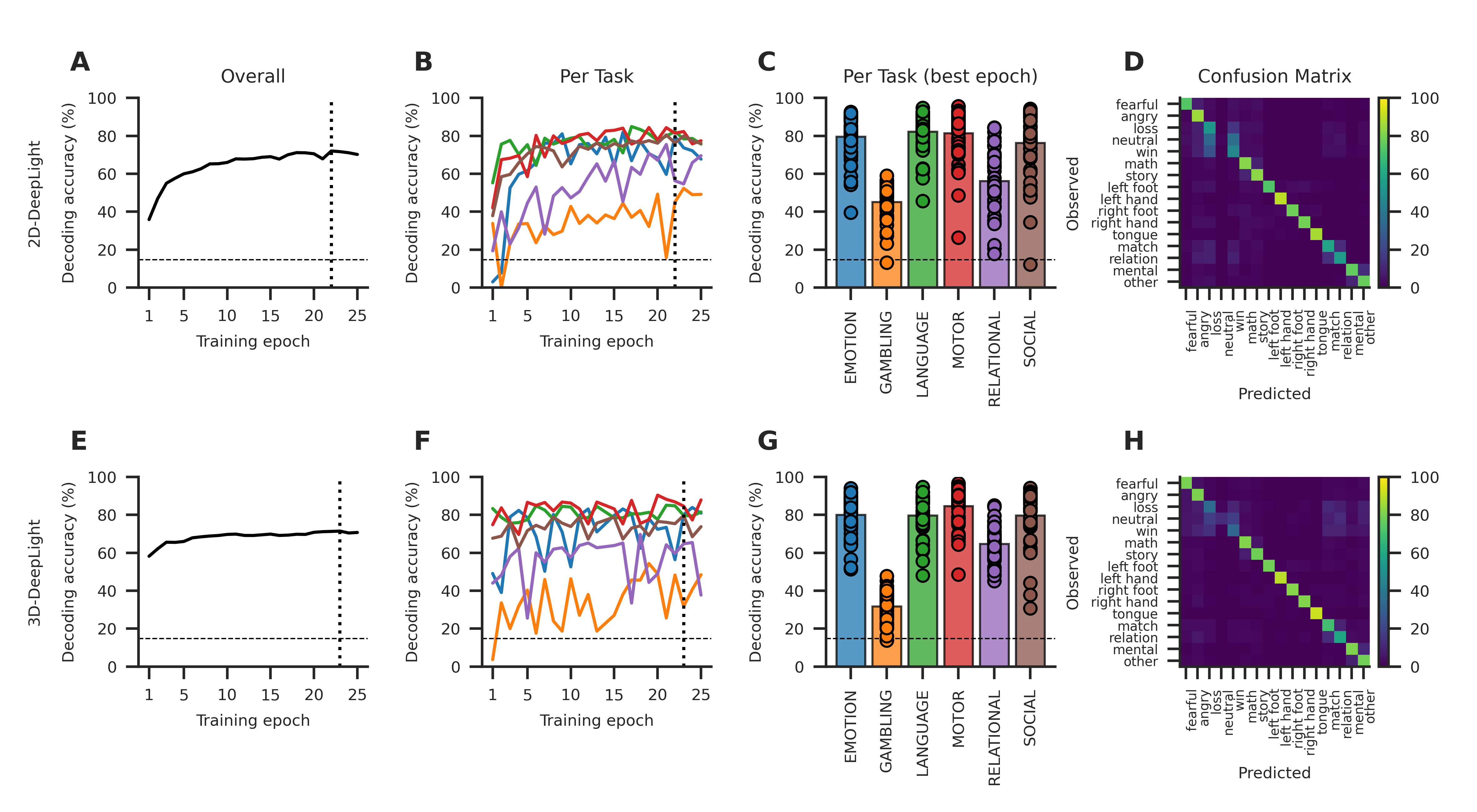
During pre-training, the output layer of both DeepLight architectures contained 16 units, one for each cognitive state of each task in the pre-training dataset (for an overview of the individual cognitive states, see Table 1). The DeepLight architectures therefore had no knowledge of the number of experimental tasks in the dataset and the assignment of cognitive states to each task. Both architectures were solely trained to identify the 16 cognitive states from single TRs. We trained each DeepLight architecture for a period of 25 epochs of stochastic gradient descent (Fig. 3 A, E; for details on the training procedures, see section 4.3). Each epoch was defined as an iteration over the entire training data of the pre-training dataset.
Both DeepLight architectures performed well in decoding the cognitive states from the fMRI data of the pre-training dataset (at a chance level decoding accuracy of ; Fig. 3 A, E): 2D-DeepLight achieved its highest decoding accuracy in the validation data after 22 training epochs (; Fig. 3 A), whereas 3D-DeepLight achieved its highest validation decoding accuracy after 23 training epochs (; Fig. 3 E). Note that these performances were statistically not meaningfully different from one another for the 50 subjects in the validation data of each of the six experimental tasks in the pre-training dataset (). Importantly, we used the parameter estimates from the training epochs at which each DeepLight architecture performed best in the validation data (i.e., 22 for 2D-DeepLight and 23 for 3D-DeepLight; Fig. 3 A, E) for all subsequent analyses involving the pre-trained models.
Both DeepLight architectures generally performed best at identifying the cognitive states of the ”motor” (2D: , 3D: ; Fig. 3 B-C, F-G), ”language” (2D: , 3D: ; Fig. 3 B-C, F-G), ”emotion” (2D: , 3D: ; Fig. 3 B-C, F-G), and ”social” (2D: , 3D: ; Fig. 3 B-C, F-G) HCP experimental tasks (see Fig. 3 B-C, F-G). They did not perform as well in the ”relational” experimental task (2D: , 3D: ; Fig. 3 B-C, F-G) and generally struggled to accurately decode the cognitive states of the ”gambling” task (2D: , 3D: ; Fig. 3 B-C, F-G).
Interestingly, both architectures exhibited little confusion between the cognitive states of different experimental tasks (with the exception of the gambling task; see Fig. 3 D, H), indicating that they were able to correctly group the cognitive states of the tasks without receiving any explicit information about the task structure during training.
2.3 Pre-trained models transfer well to an independent experimental task
Both pre-trained DeepLight architectures (2D and 3D; see Fig. 2) accurately decode the cognitive states of the pre-training dataset (see Fig. 3 C, G). Next we were therefore interested in evaluating whether they perform better at identifying the four cognitive states of the left-out HCP experimental task (the ”working memory” task; see section 4.1.1) when compared to respective model variants that are trained from scratch. In the HCP-working memory task (HCP-WM), individuals viewed images of body parts, faces, places, and tools in the fMRI. The target of the decoding analysis was to identify these four cognitive states from individual TRs.
2.3.1 Allowing the pre-trained weights to change during fine-tuning is beneficial
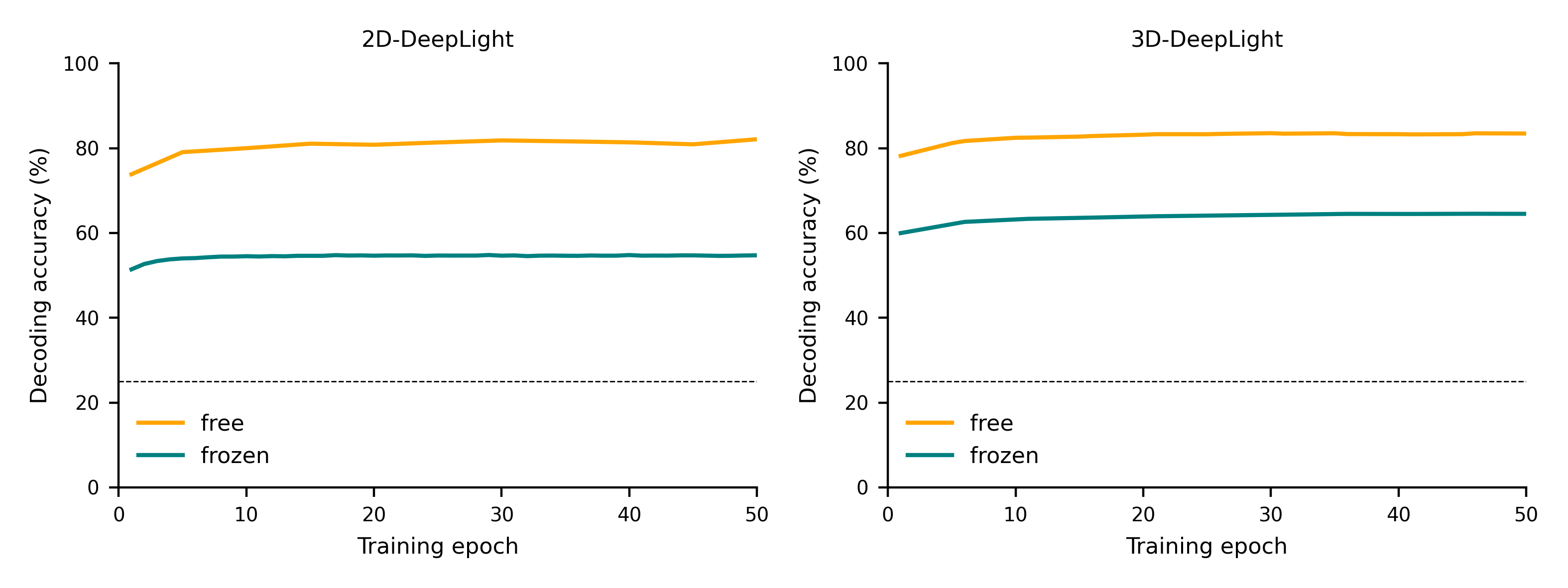
In a first step of this analysis, we compared the performance of two common fine-tuning approaches, by testing whether a model that freezes the pre-trained weights during fine-tuning (e.g., Rajaraman et al.,, 2018) performs better than a model variant that continues to train these weights (e.g., Samek et al., 2017a, , Thomas et al., 2019b, ). To do this, we first initialized the weights of two identical variants of each architecture (for an overview of the model architectures, see Fig. 2 and section 4.2) to the weights of the pre-trained models (except for weights of the output layers, which now included four instead of 16 units; see section 4.2). We then held the pre-trained weights of one variant of each architecture constant during fine-tuning, while we allowed the weights of the respective other variant to change.
After 50 training epochs (for an overview of the training procedures, see section 4.3), the model variants whose weights were allowed to change clearly outperformed the model variants with frozen weights (see Appendix Fig. B.1): While the models with frozen weights achieved final decoding accuracies of (2D) and (3D) in the validation data of the HCP-WM task, model variants that were allowed to change these weights achieved a final decoding accuracy of (2D) and (3D). We therefore allowed the pre-trained models to change their weights during fine-tuning in all further transfer learning analyses.
2.3.2 Pre-trained models decode more accurately than models trained from scratch
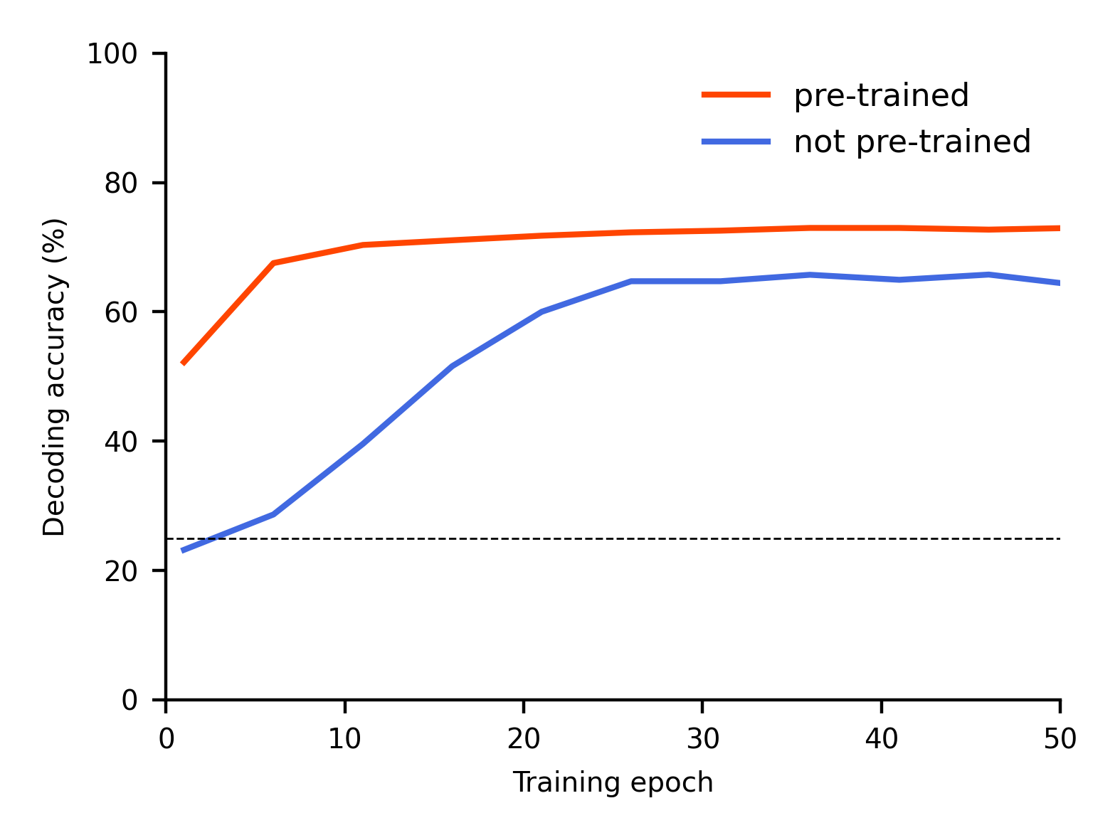
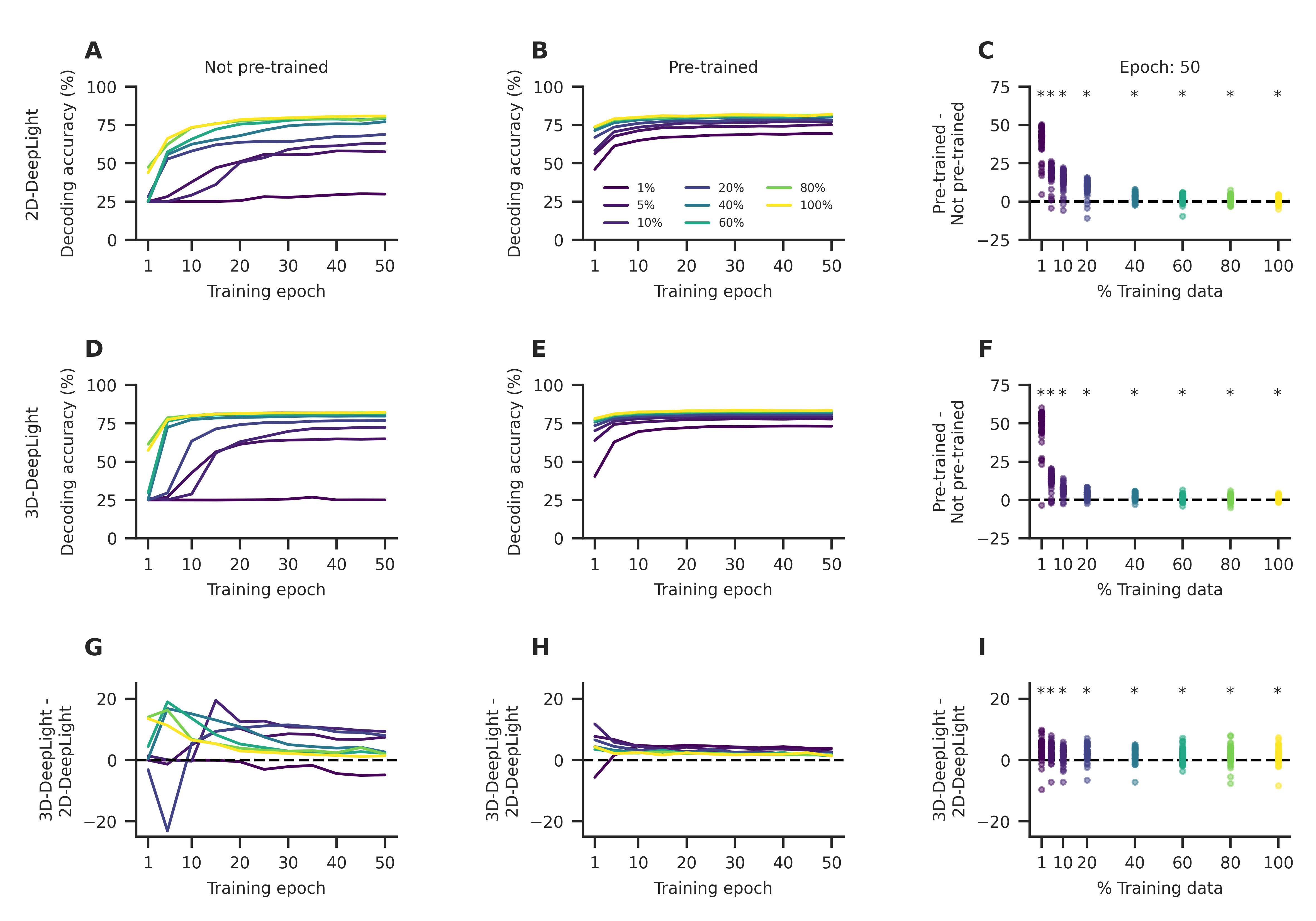
In a second step of this analysis, we then compared the performance of the pre-trained models to those of two model variants that were trained from scratch (with weights initialized according to the random uniform initialization scheme proposed by Glorot and Bengio,, 2010). After 50 training epochs, the model variants that were not pre-trained achieved a final decoding accuracy of (2D; Fig. 4 A) and (3D; Fig. 4 D) in the validation data of the HCP-WM task, thereby performing () and () worse than their pre-trained counterparts (Fig. 4 C, F)).
To also test how the pre-trained and not pre-trained model variants compared when applied to smaller fractions of the full training dataset of the HCP-WM task (N = 400), we trained both variants of each architecture on the data of 1%, 5%, 10%, 20%, 40%, 60%, and 80% of the full training dataset. Importantly, we always evaluated the decoding performance of each model on the data of all 50 subjects in the validation dataset.
The pre-trained DeepLight variants consistently achieved higher decoding accuracies than the models that were not pre-trained (Fig. 4 C, F). Note that the pre-trained models were able to correctly identify the cognitive state underlying (2D) and (3D) of the fMRI volumes of the validation dataset, when they were trained with only 1% of the training dataset (equal to a dataset of four subjects). The DeepLight variants that were not pre-trained, on the other hand, achieved a decoding accuracy of (2D) and (3D) when trained on 1% of the training data (thereby performing meaningfully worse than their pre-trained counterparts; the difference in decoding accuracy between the pre-trained and not pre-trained models was , () and () for the 2D- and 3D architectures respectively).
Similarly, the pre-trained DeepLight variants that were fine-tuned on 40% of the training dataset achieved a final decoding performance that was as good as the performance of the DeepLight variants that were trained from scratch on the data of all 400 subjects in the training dataset (2D: (not pre-trained; 100%) (pre-trained; 40%) = (), 3D: (not pre-trained; 100%) (pre-trained; 40%) = (); Fig. 4 A-B, D-E)
Overall, the 3D-DeepLight variants were slightly more accurate in identifying the cognitive states from the fMRI data than their 2D counterparts (Fig. 4 G - I). While the 3D-DeepLight variants generally also learned faster (by achieving higher decoding accuracies earlier in the training; Fig. 4 G-H), we refrain from interpreting this finding further, as we used slightly different learning rates to train the two DeepLight architectures (for details on the training procedures, see section 4.3).
2.4 Pre-trained models transfer well to an independent fMRI dataset
Our analyses have shown that the pre-trained DeepLight variants consistently achieve higher decoding accuracies than model variants that were not pre-trained when both are applied to the fMRI data of the HCP-WM task. To also test whether the pre-trained models exhibit a similar advantage in decoding performance when applied to an independent fMRI dataset that is not part of the HCP, we performed a similar transfer learning analysis on a dataset that was originally published by by Nakai and Nishimoto (the ”Multi-task” dataset; Nakai and Nishimoto,, 2020). In this dataset, six participants repeatedly performed 103 simple naturalistic tasks in the fMRI (e.g., deciding whether the music that is currently being played is Jazz or whether there is a penguin on a presented image; for further details on the tasks and dataset, see section 4.1.2 and Nakai and Nishimoto,, 2020). In total, the Multi-task dataset contains the fMRI data of 18 runs for each individual and is split into a training dataset (containing the data of 12 runs per individual) and a test dataset (containing the data of the remaining six runs per individual). In the test runs, participants performed versions of the 103 tasks that were not included in the training runs (for example, by utilizing different music or images). Similar to our previous analyses, we evaluated the performance of a pre-trained and not pre-trained variant of each DeepLight architecture (2D and 3D; see Fig. 2) in identifying the 103 tasks (i.e., cognitive states) from the fMRI data of this dataset (for an overview of the training procedures, see section 4.3).
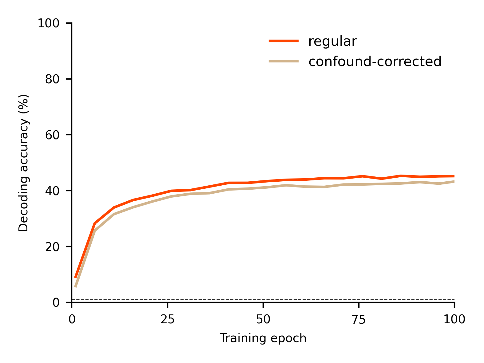
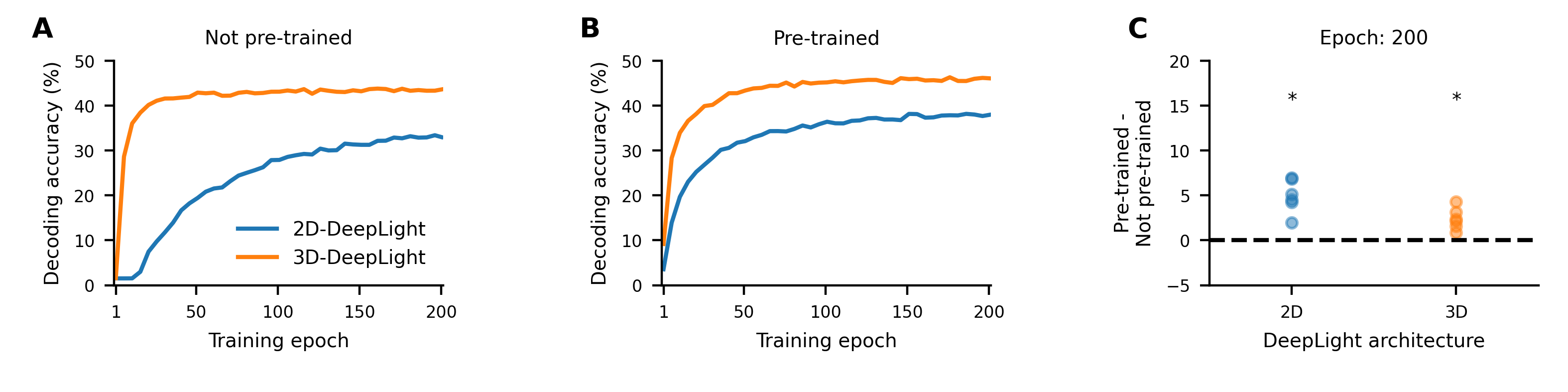
Both pre-trained DeepLight variants again outperformed their not pre-trained counterparts at identifying the 103 tasks from the fMRI data (Fig. 5), while the 3D-DeepLight variants performed better than the respective 2D-DeepLight variants (Fig. 5 A-B). After 200 training epochs, the 2D-DeepLight variant that was not pre-trained achieved a final decoding accuracy of in the test runs of the Multi-task dataset (blue line in Fig. 5 A), while the not pre-trained 3D-DeepLight variant achieved a final decoding accuracy of (orange line in Fig. 5 A). The pre-trained DeepLight variants, in contrast, achieved a final decoding accuracy of (2D; Fig. 5 B) and (3D; Fig. 5 B) respectively. The pre-trained variants therefore outperformed their not pre-trained counterparts by (; 2D) and (; 3D), while the 3D-DeepLight variants outperformed the 2D variants by (; not pre-trained) and (; pre-trained).
Interestingly, the pre-trained 3D-DeepLight variant did not exhibit the same advantages in learning speed over its not pre-trained counterpart that we observed in our previous analyses, as both exhibited similar increases in decoding accuracy per training epoch (Fig. 5 A-B). We thus confirmed in a sequence of additional analyses that the transfer performance of the pre-trained 3D-DeepLight variant to the Multi-task dataset was not affected by any basic differences in the statistical properties, noise or preprocessing between the HCP and Multi-task datasets (see Appendix B.1).
2.5 Pre-trained models reuse features when trained on new data
To better understand the mechanisms giving rise to the advantages in decoding performance and learning speeds of the pre-trained models that we observed (see Fig. 4 and Fig. 5), we next analyzed their hidden layer representations. We would assume that the pre-trained models are generally able to learn quicker and from less data because they reuse many of their learned features when training on a new dataset (c.f., Neyshabur et al.,, 2020). Accordingly, the hidden layer representations of the pre-trained models should be highly similar for a new dataset before and after training on the dataset. In contrast, the hidden representations of models that were not pre-trained should be more dissimilar, as their learned features are solely informed by the dataset at hand.
To test these hypotheses, we compared the similarity of the hidden layer representations between three types of models: those that were pre-trained on the data of the six HCP pre-training tasks (see section 2.2), those that were pre-trained and then fine-tuned on either of the two fine-tuning datasets (namely the HCP-WM and Multi-task datasets; see section 2.3), and those that were trained on these fine-tuning datasets without any pre-training (thus with randomly initialized weights). In the following, we will indicate these three different model types with P (pre-trained), P-F (pre-trained and fine-tuned), and R-F (trained with randomly initialized weights).
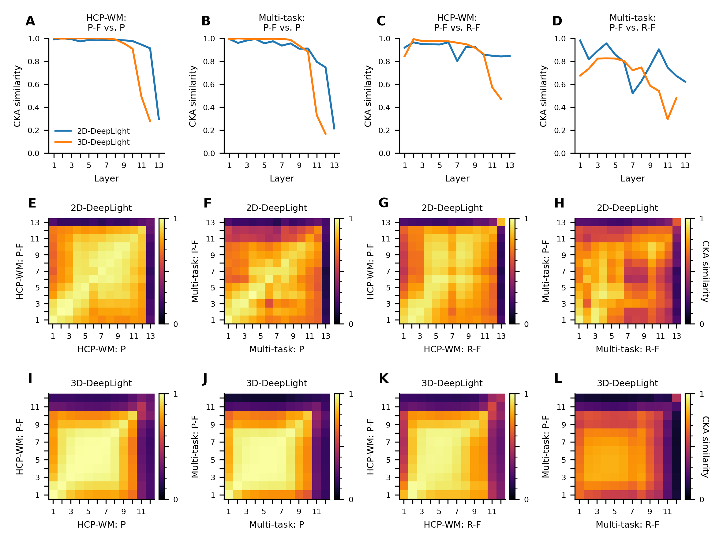
To quantify the similarity between the hidden layer representations of two models, we utilized the centered kernel alignment index (CKA; using a linear kernel), which was recently proposed by Kornblith et al., (2019) (see also Braun et al.,, 2008, Cristianini et al.,, 2001, Montavon et al.,, 2011). By the use of this similarity index, we computed a similarity matrix for each model comparison, indicating the similarity between the hidden representations of each pair of layers from the two models (see Fig. 6 E-L). To compute the similarity of two layers’ representations, we first extracted their representations of each fMRI volume of a subject in a dataset and then used these representations to compute the CKA similarity for the data of that subject. To obtain an overall estimate of representation similarity, we next averaged these individual subject similarities over all subjects in a dataset. Note that we restricted this analysis to only those model layers whose weights were also transferred from the pre-trained models during fine-tuning (thus excluding the output layers of both DeepLight architectures; see Fig. 2 and section 4.2). We also averaged the representations of convolution layers over their kernel dimension to compensate for their otherwise very high dimensionality.
By the use of this analysis strategy, we first compared the hidden layer representations of P and P-F models for the data of the HCP-WM (Fig. 6 A, E, I) and Multi-task datasets (Fig. 6 B, F, J). This comparison revealed that the hidden representations of P models are generally very similar to those of P-F models in both datasets, indicating that P models reuse many of their learned features during fine-tuning; as we hypothesized.
In contrast, the hidden representations of R-F models are generally more dissimilar to those of P-F models (Fig. 6 C-D), demonstrating that R-F models use a more dissimilar set of features to decode the cognitive states of the two datasets; Again, as we hypothesized.
Interestingly, the similarity of the hidden representations in all model comparisons generally decreased for later layers of both DeepLight architectures (i.e., 2D-DeepLight’s LSTM layer and 3D-DeepLight’s last two layers of the convolutional feature extractor; Fig. 6 A-D). The representations of these layers were also highly dissimilar to the representations of all other model layers (Fig. 6 E-L). This suggests that these higher-level features are more specific to each model and set of cognitive states in a dataset and that they therefore do not generalize as well across datasets as the lower-level features which are closer to the input data.
2.6 Pre-trained models utilize unforeseen mappings between cognitive states and brain activity
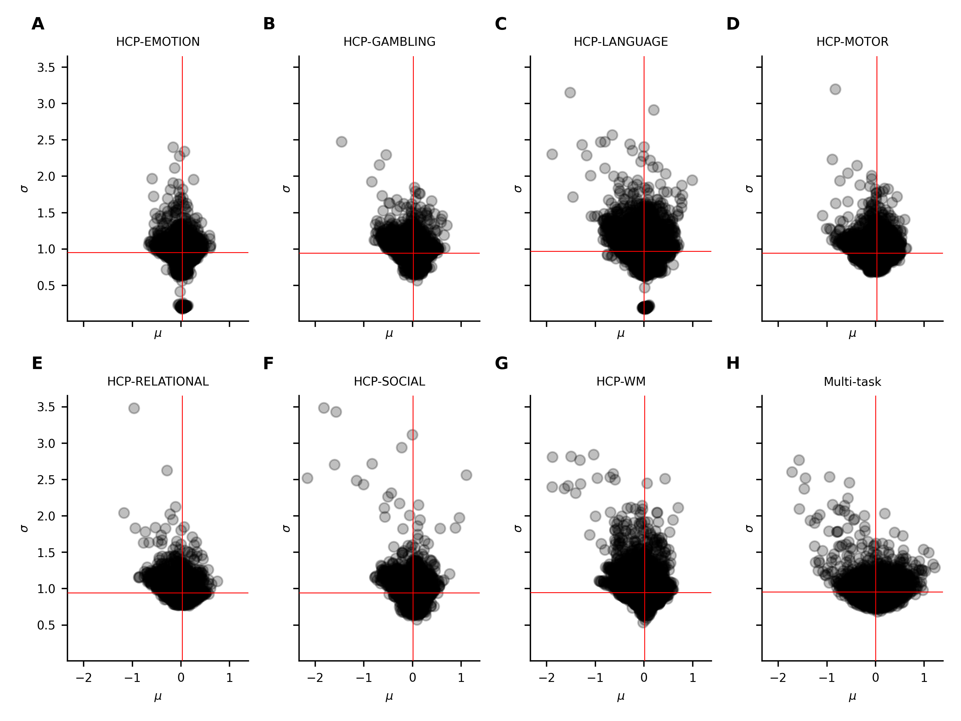
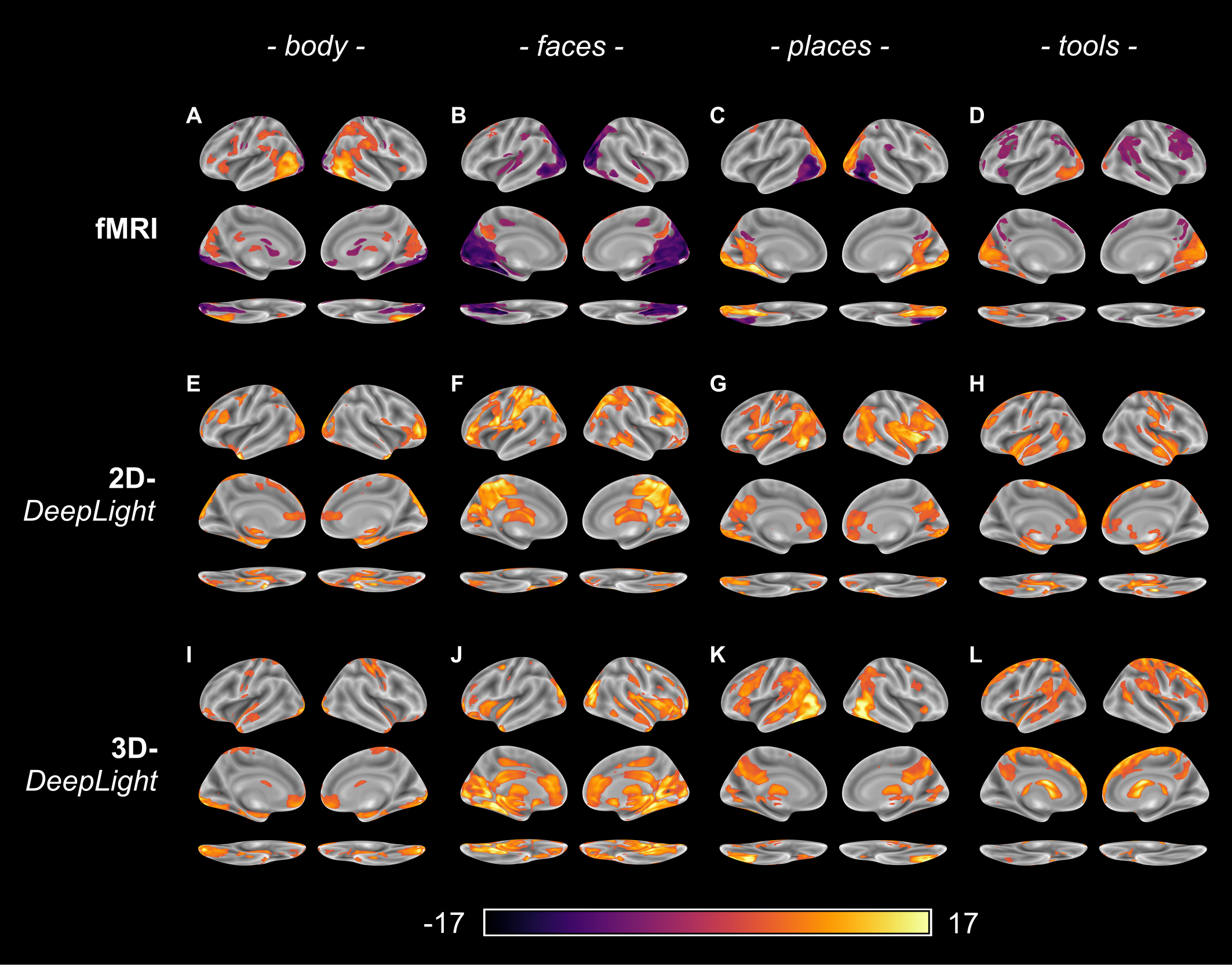
Our findings demonstrate that the two pre-trained DeepLight variants consistently achieve higher decoding accuracies than their not pre-trained counterparts, while generally also learning quicker and requiring less training data (see sections 2.2, 2.3, and 2.4). Our results also indicate that these advantages arise from the ability of the pre-trained models to reuse many of their learned features when training with new data. To better understand the mappings between brain activity and cognitive states that the pre-trained models utilize, we next interpreted their decoding decisions with the LRP technique (for details on the LRP interpretation, see section 4.4) for the validation data of the pre-training dataset (comprising 50 subjects in each of six HCP experimental tasks; see section 4.1.1). For comparison, we also performed a standard two-stage GLM analysis (Holmes and Friston,, 1998) of the same fMRI data, contrasting each cognitive state of an experimental task against all other states of the task (for details on the GLM analysis, see Appendix A.2). Since LRP interpretation results in a dataset of equal dimension as the original input data (with one relevance value for each input voxel), we performed a similar two-stage GLM analysis of the relevance data of each experimental task to identify the brain regions that the pre-trained models associate most strongly with each cognitive state (thus restricting the results of this analysis to only positive z-scores) (for details on the GLM analysis, see Appendix A.2). All GLM analyses were performed on parcellated brain data, comprising a set of 256 brain networks that were extracted from each fMRI volume by the use of the dictionaries of functional modes (DiFuMo) atlas. These 256 brain networks are optimized to represent fMRI data well across a wide range of experimental conditions (for methodological details on the DiFuMo atlas, see Dadi et al., (2020)). Note that we excluded the data of the HCP-gambling task from this analysis, as the pre-trained models did not perform well in decoding the cognitive states of this task (see Fig. 3 C,G).
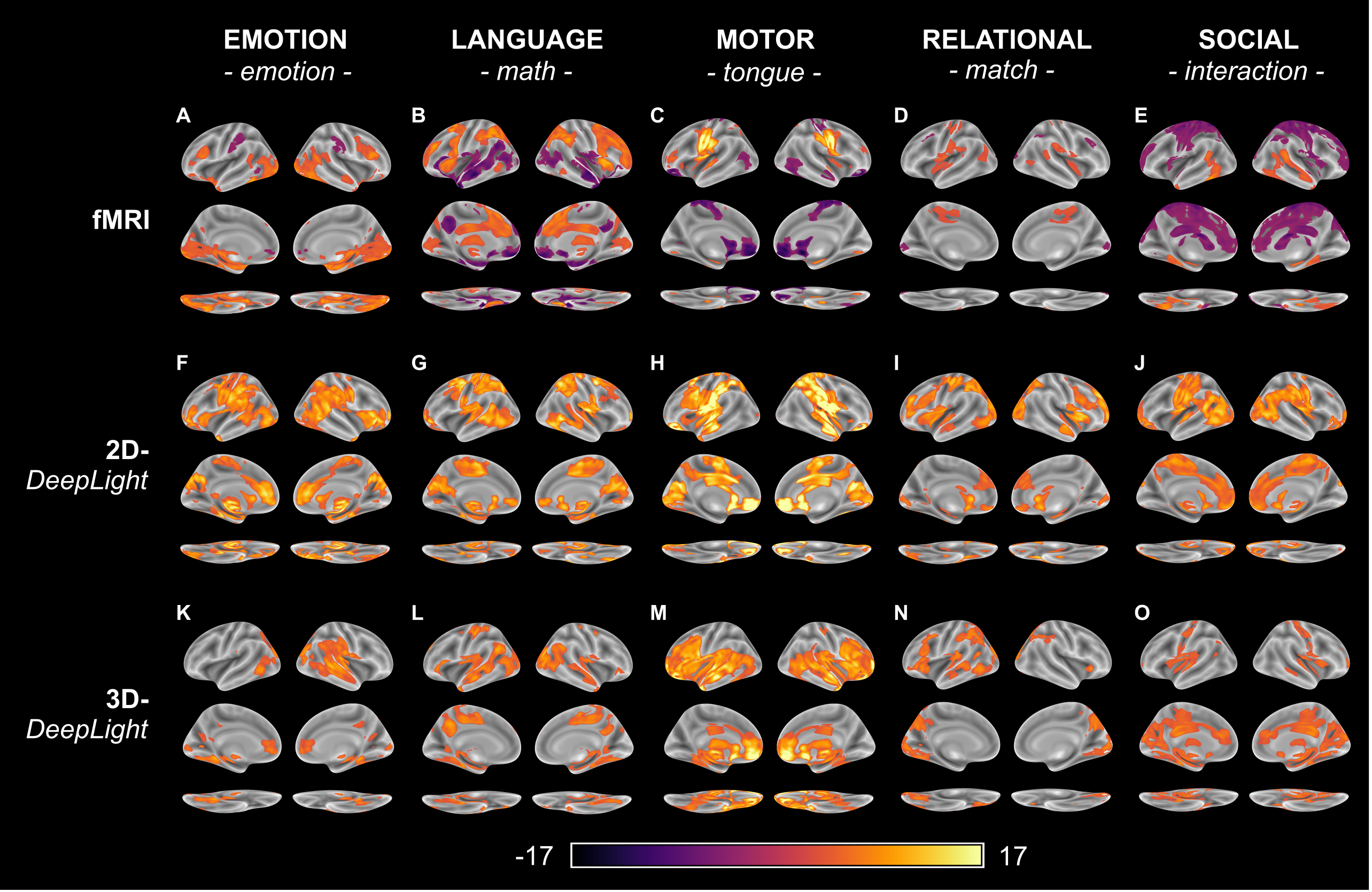
Figure 7 provides an overview of the results of this analysis and depicts the brain maps (thresholded at a false-discovery rate of 0.001) for one exemplary cognitive state of each experimental task, namely, the ”emotion” state of the HCP-emotion task, in which individuals see images of angry or fearful faces, the ”math” state of the HCP-language task, in which individuals solve arithmetic problems, the ”tongue” state of the HCP-motor task, in which individuals move their tongue, the ”match” state of the HCP-relational task, in which individuals decide if visually presented objects match on a given dimension, and the ”interaction” state of the HCP-social task, in which individuals saw objects in a video clip that interacted in some way (for further details on the HCP experimental tasks, see section 4.1.1 and Appendix A.1).
In general, the two pre-trained DeepLight variants associated a similar overall set of brain regions with these cognitive states as our GLM analysis of the fMRI data. Yet, their learned mappings between brain activity and the individual cognitive states are, at first sight, surprising and counterintuitive given the results of the fMRI-GLM analysis (Fig. 7 A-E). Take as an example the ”tongue” state of the HCP-motor task (Fig. 7 C,H,M). The fMRI-GLM analysis (Fig. 7 C) indicates that the lower parts of the primary motor and somatosensory cortices exhibit overall stronger activation in this state when compared to movements of fingers or toes (the other cognitive states of the HCP-motor ask). While 2D-DeepLight (Fig. 7 H) also utilizes the activity of these regions to identify tongue movements, 3D-DeepLight (Fig. 7 M) does not take the activity of these regions into account when identifying movements of the tongue. Instead, both DeepLight variants focus more strongly on the activity of the ventromedial prefrontal and anterior cingulate cortices when decoding tongue movements. These regions are, however, not positively associated with tongue movements in the fMRI-GLM analysis (Fig. 7 C). To make sense of this mapping, we need to look back at the results of the fMRI-GLM analysis (Fig. 7 C), which indicate that the ventromedial prefrontal and anterior cingulate cortices exhibit overall less activation during tongue movements relative to the other movements of the HCP-motor task. The two pre-trained DeepLight variants have thus learned to associate the relatively lessened activity of these regions with movements of the tongue.
A similar pattern can be observed for the ”math” state of the HCP-language task (Fig. 7 B,G,L). The fMRI-GLM analysis (Fig. 7 B) indicates that the superior temporal gyrus is generally less active when individuals solve arithmetic problems, when compared to answering questions about brief fables (the other cognitive state of the HCP-language task). Again, both DeepLight variants (Fig. 7 G,L) interpret this lessened activity as evidence for the presence of the ”math” state, as indicated by the generally higher relevance values in this region. Interestingly, both DeepLight variants do not take into account the generally higher activation of the anterior cingulate cortex in this cognitive state (Fig. 7 B), demonstrating that the set of brain regions that the models associate with individual cognitive states does not fully overlap with the set of brain regions identified by the fMRI-GLM analysis.
Note that the two DeepLight variants also slightly differ in the specific set of brain regions whose activity they associate with the individual cognitive states. For example, when decoding the ”interaction” state of the HCP-social task (Fig. 7 E,J,O), 2D-DeepLight (Fig. 7 J) focuses on activity of the posterior parts of the superior and medial temporal gyri as well as the lateral occipital cortex, whereas 3D-DeepLight (Fig. 7 O) does not associate these brain regions with this state and instead focuses on activity of the medial parts of the occipital cortex as well as the posterior cingulate cortex.
Summarizing, this analysis shows that while the two pre-trained DeepLight variants associate a similar overall set of brain regions with the cognitive states of the HCP experimental tasks as a standard GLM analysis of the same data, the specifics of their learned mapping between individual states and brain activity are unforeseen and counterintuitive, as they have learned to identify individual cognitive states through the combined activity of brain regions that are generally less active in these states relative to other cognitive states and regions that are relatively more active (much like a ”Clever Hans”; Lapuschkin et al.,, 2019). In addition, our results show that two DL models can differently utilize the activity of the same set of brain regions to decode the same set of cognitive states with similar accuracy.
To ensure that these findings are not specific to the pre-training dataset, we replicated this analysis for the data of the 50 subjects in the validation dataset of the HCP-WM task (see Appendix Fig. B.5), using the pre-trained models that were fine-tuned on the full training dataset of that task (see section 2.3). This analysis revealed similar patterns in the model’s learned mappings between brain activity and cognitive states, as both pre-trained DeepLight variants associate a similar overall set of brain regions with the cognitive states of the HCP-WM task as a standard GLM analysis of the fMRI data, while identifying individual cognitive states through the combined activity of brain regions that are relatively more active in these states and regions that are relatively less active. For example, the fMRI-GLM analysis (Appendix Fig. B.5 B-C) indicates generally reduced activation of the parahippocampal gyrus (also known as the parahippocampal place area PPA; Heekeren et al., (2004)) in the ”faces” state, relative to the other cognitive states of the HCP-WM task, and similarly reduced activation of the fusiform gyrus (also known as the fusiform face area FFA; Heekeren et al., (2004)) in the ”places” state. In line with this activity pattern, 3D-DeepLight (Appendix Fig. B.5 J-K) associates the ”faces” state with reduced activation of the PPA and the ”places” state with reduced activation of the FFA, assigning higher relevance values to these regions when decoding these states. At first sight, 3D-DeepLight’s brain maps therefore seem directly at odds with the results of the fMRI-GLM analysis and a wealth of other empirical findings for this task (e.g., Heekeren et al.,, 2004, Haxby et al.,, 2000), which clearly associate stronger activity of the FFA with the viewing of faces and stronger activity of the PPA with the viewing of places. Only by interpreting 3D-DeepLight’s brain maps in the context of the results of the GLM analysis of the underlying fMRI data, we can uncover that this seemingly contradictory mapping is in fact biologically plausible and in line with the activity patterns of the fMRI data.
3 Discussion
In this work, we systematically evaluated deep transfer learning for cognitive decoding from whole-brain functional neuroimaging data. We first trained two distinct DL model architectures on a large whole-brain fMRI dataset of the HCP (Uğurbil et al.,, 2013) and subsequently evaluated their performance in decoding the cognitive states of an independent experimental task and dataset. The pre-trained models consistently achieved higher decoding accuracies than model variants that were not pre-trained while generally also learning quicker and requiring less training data, underlining the overall benefits of pre-training.
Our findings suggest that these advantages result from the ability of the pre-trained models to reuse the features that they have learned during pre-training when training on a new dataset. This finding is in line with recent empirical work in computer vision, demonstrating that DL models, which start their training from pre-trained weights, generally exhibit highly similar features before and after training on other datasets (Neyshabur et al.,, 2020). Here, researchers assume that the pre-trained models stay in the same basin of the loss function when trained on new data, leading to similar learned features and overall quicker convergence on a solution to the learning task. Models that are trained from scratch, on the other hand, start their training with randomly initialized weights and thus generally require more training time to learn a set of viable features, as these features are solely informed by the training dataset at hand. Our findings generally support these notions, as the pre-trained models achieve higher overall decoding accuracies in the two validation datasets, generally learn quicker, and exhibit highly similar features before and after training on the two validation datasets, when compared to model variants that are not pre-trained.
In our analyses, the feature reuse of the pre-trained models was mostly restricted to lower-level features, which are closer to the input data, as the hidden representations of layers that are deeper in the models differed more strongly between the different applications of the models. This indicates that these lower-level features generalize better between datasets by providing a more general projection of the fMRI data into a lower-dimensional space, which preserves important variance of the brain activity (c.f., Braun et al.,, 2008, Montavon et al.,, 2011). The higher-level features, in contrast, are aimed at discriminating a specific set of cognitive states from this lower-dimensional representation (e.g., by suppressing features that are not of interest; Haufe et al.,, 2014) and are therefore more specific to a dataset and model.
We also found that the 2D-DeepLight architecture consistently achieved slightly lower decoding accuracies than its 3D counterpart. 2D-DeepLight is inspired by recent work in computer vision for video data (e.g., Donahue et al.,, 2017, Marban et al.,, 2019), where the combination of 2D-convolution and recurrent neural network unit is often beneficial over the application of 3D-convolutions to the image sequences. Here, such 2D-architectures can explicitly account for the contents of each image of a sequence, while also accounting for the changes from each image to the next. For fMRI data, however, 2D-DeepLight creates an artificial separation between the axial slices of an fMRI volume. This makes the decoding of cognitive states potentially more challenging than for 3D-DeepLight, which directly operates in the volumetric space of fMRI.
In contrast to other recent empirical work utilizing DL models for the decoding of fMRI data (e.g., Zhang et al.,, 2021), DeepLight does not specifically account for the temporal evolution of brain activity, as it processes individual fMRI volumes independently from one another. In theory, this is a strongly limiting assumption, as understanding the temporal dynamics of brain activity is fundamental to understanding the dynamics of the brain. To explicitly account for the temporal evolution of brain activity, DeepLight can be extended with another recurrent network layer, which takes as input the higher-level representations of whole-brain activity resulting from any of the two DeepLight architectures used in this work. Recent empirical work has already demonstrated that 2D-DeepLight’s relevance values follow the temporal evolution of the haemodynamic response measured by fMRI Thomas et al., 2019a , suggesting that it captures the measured brain signal well at each time point. The two pre-trained DeepLight architectures that we publish with this work thus provide promising starting points for such an extended DeepLight architecture that specifically accounts for the temporal evolution of the fMRI signal.
Our findings also point towards nuanced challenges for the application of DL models to the decoding of cognitive states from whole-brain functional neuroimaging data. When interpreting the decoding decisions of the two pre-trained DeepLight variants for the fMRI data of six out of the seven HCP experimental tasks (excluding the HCP-gambling task), we found that both models generally associated a similar overall set of brain regions with the cognitive states of these tasks as a standard two-stage GLM analysis of the fMRI data (see Fig. 7 and Appendix Fig. B.5). Surprisingly, they learned to identify individual cognitive states through the activity of brain regions that are generally less active in these states in combination with the activity of regions that are generally more active in these states. At first sight, the resulting brain maps can therefore seem at odds with the results of the standard GLM analysis of the same data, as the pre-trained models assign high relevance to brain regions that the GLM analysis negatively associates with these states. Yet, the learned mappings of the pre-trained models are in fact biologically plausible, given the underlying decoding task. Cognitive decoding analyses are aimed at characterizing the representations of a brain region by identifying the cognitive states that can be reliably identified from the activity of the region (c.f. Norman et al.,, 2006). Knowing that a particular brain region is consistently less active in a particular cognitive state (relative to other states) is therefore similarly informative about the representations of this region as knowing that it is consistently more active in other states.
More generally, an interpretation of the cognitive decoding decisions of DL models allows us to identify brain networks whose activity is associated with the decoded cognitive states. Yet, the interpretation does not necessarily indicate the characteristics of the mapping between the activity of these networks and the cognitive states. To accurately characterize this mapping, it is essential to compare the results of the interpretation analysis to those of other analysis approaches for the same data as well as related empirical findings. DL models are extremely powerful representation learners (for a detailed discussion, see Goodfellow et al.,, 2016, LeCun et al.,, 2015), which have been shown to often learn mappings between input data and target signal that are not foreseen by the researchers training these models (e.g., Geirhos et al.,, 2020, Lapuschkin et al.,, 2019, Oakden-Rayner et al.,, 2020, McCoy et al.,, 2019, Zech et al.,, 2018). Their learned mappings therefore need to be interpreted with caution, when aiming to draw inferences about the association between brain activity and cognitive states.
Relatedly, our analyses have shown that two DL models, which achieve similar overall decoding performances, can differ in how they combine the activity of the same set of brain regions to distinguish the same set of cognitive states. This suggests that DL models are able to adopt multiple different solutions for the mapping between a set of cognitive states and brain activity that allow them to perform similarly well on average. While this finding might seem trivial at first, it has far-reaching consequences, as it brings forward questions about the reproducibility of inferences about the mapping between brain activity and cognitive states that are drawn from the interpretation of cognitive decoding decisions of DL models. Recent empirical work in DL research has demonstrated that the convergence of DL models, and thereby the specifics of their learned mapping between input data and target signal, is dependent on many non-deterministic aspects of the training process, such as random seeds and random weight initializations (Henderson et al.,, 2018, Lucic et al.,, 2018, Reimers and Gurevych,, 2017, Dodge et al.,, 2019) as well as the specific choices for other hyper-parameters, such as individual layer specifications and optimization algorithms Melis et al., (2017), Zoph and Le, (2017), Lucic et al., (2018). It is thus possible that the mapping between cognitive states and brain activity that a DL model learns can change with these factors of the training. In line with other researchers (Bouthillier et al.,, 2021, Dodge et al.,, 2019, Thomas et al.,, 2021), we therefore urge researchers who are interested in drawing inferences about the mapping between cognitive states and brain activity from an interpretation of the cognitive decoding decisions of DL models to test for the influence of convergence on the models’ learned mappings, for example, by repeatedly training the same model on the same dataset while varying different non-deterministic aspects of the training (e.g., random seeds, random weight initialzations, and random shufflings and augmentations of the training data) as well as other hyper-parameters (e.g., batch sizes, individual layer specifications, learning rates), and to study the effect of these variations on the model’s learned mapping between brain activity and cognitive states.
In conclusion, this work clearly underlines the overall benefits of pre-training for the application of DL models to cognitive decoding from whole-brain fMRI data, as pre-trained models generally exhibit higher decoding accuracies and require less training time and data when compared to model variants that are not pre-trained. Yet, this work also surfaces nuanced challenges that arise for the application of DL models to whole-brain decoding, as the mappings between brain activity and cognitive states that DL models learn can be unforeseen and counterintuitive, and thus require careful additional analysis to be understood well.
4 Methods
4.1 Overview of datasets and experimental tasks
4.1.1 Human Connectome Project
| Task | Cognitive states | Count | Duration (min) |
|---|---|---|---|
| WM | body, face, place, tool | 4 | 5:01 |
| Gambling | win, loss, neutral | 3 | 3:12 |
| Motor | left/right finger, left/right toe, tongue | 5 | 3:34 |
| Language | story, math | 2 | 3:57 |
| Social | interaction, no interaction | 2 | 3:27 |
| Relational | relational, matching | 2 | 2:56 |
| Emotion | emotion, neutral | 2 | 2:16 |
| Total | 20 | 23:03 |
The task-fMRI data of the Human Connectome Project (Barch et al.,, 2013) includes seven tasks that were each performed in two separate runs (for a general overview, see Table 1). For each task, participants were first provided with detailed instructions outside of the fMRI and only given a very brief reminder of the task and a refresher on the response button box mappings before the start of each task in the fMRI. We briefly summarize each experimental task in the following, while a more detailed description of the tasks can be found in Appendix A.1.
Working memory (WM):
Participants were asked to decide in an N-back task whether a currently presented image (of body parts, faces, places or tools) is the same as a previously presented target image. The target image was either presented at the beginning of the experimental block (0-back) or participants were asked to decide whether the currently presented image is the same as the one presented two before (2-back).
Gambling:
Participants were asked to guess whether the value of a card (with values between 1-9) is below or above 5. Participants won or lost if they guessed correctly/incorrectly. Trials were neutral if the value of the card was 5. The number on the card was dependent on whether the respective trial belonged to the reward, loss, or neutral task condition.
Motor:
Participants were presented with visual cues asking them to tap their left or right fingers, squeeze their left or right toes, or move their tongue.
Language:
Participants either heard a brief fable (story trials) or an arithmetic problem (math trials) and were subsequently given a two-alternative question about the story or arithmetic problem.
Social:
Participants were presented with short video clips of objects that either interacted in some way (interaction trials) or moved randomly (no interaction trials). Subsequently, participants were asked to decide whether the objects interacted with one another, did not have an interaction, or if they are not sure.
Relational:
Participants were presented with different shapes, filled with different textures. In relational trials, participants saw a pair of objects at the top of the screen and a pair at the bottom. They were then asked to decide whether the bottom pair differs along the same dimension (shape or texture) as the top pair. In match trials, participants saw one object at the top and bottom and were asked to decide whether the objects matched on a given dimension.
Emotion:
In emotion trials, participants were asked to decide which of two faces presented on the bottom of the screen matches the face at the top of the screen (faces had an either angry or fearful expression). In neutral trials, participants were asked to to decide which of two shapes at the bottom of the screen matches a shape that is presented at the top.
fMRI data for each task were provided in a preprocessed format by the Human Connectome Project (HCP S1200 release), WU Minn Consortium (Principal Investigators: David Van Essen and Kamil Ugurbil; 1U54MH091657) funded by the 16 NIH Institutes and Centers that support the NIH Blueprint for Neuroscience Research; and by the McDonnell Center for Systems Neuroscience at Washington University. Whole-brain EPI acquisitions were acquired with a 32 channel head coil on a modified 3T Siemens Skyra with TR = 720 ms, TE = 33.1 ms, flip angle = 52 deg, BW = 2,290 Hz/Px, in-plane FOV = 208 x 180 mm, 72 slices, 2.0 mm isotropic voxels with a multi-band acceleration factor of 8. Two runs were acquired, one with a right-to-left and the other with a left-to-right phase encoding (for further methodological details on fMRI data acquisition, see Uğurbil et al.,, 2013).
The Human Connectome Project preprocessing pipeline for functional MRI data (“fMRIVolume”; Glasser et al.,, 2013) includes the following steps: gradient unwarping, motion correction, fieldmap-based EPI distortion correction, brain-boundary based registration of EPI to structural T1-weighted scan, non-linear registration to MNI152 space, and grand-mean intensity normalization (for further details, see Glasser et al.,, 2013, Uğurbil et al.,, 2013).
In addition to the minimal preprocessing of the fMRI data that was performed by the Human Connectome Project, we applied the following preprocessing steps to the fMRI data for our decoding analyses: volume-based smoothing of the fMRI sequences with a 3mm FWHM Gaussian kernel, linear detrending and standardization of the single voxel signal time-series (resulting in a zero-centered voxel time-series with unit variance) and temporal filtering of the single voxel time-series with a butterworth highpass filter and a cutoff of 128 s, as implemented in Nilearn (Abraham et al.,, 2014).
4.1.2 Multi-task dataset
This dataset was first published by Nakai and Nishimoto, (2020) and contains the data of six healthy human participants (22-33 yrs, two female, normal vision and hearing, all right-handed) who repeatedly performed 103 simple naturalistic tasks in the fMRI (hence ”Multi-task”). These tasks were selected such that they include a variety of different cognitive domains and can be performed without previous experimental training (e.g., participants were asked whether a piece of music is Jazz or whether a penguin is shown on a a presented image; for an overview of all tasks and instructions, see Nakai and Nishimoto,, 2020). The experiment consisted of 18 fMRI runs of which 12 were designated as training runs and six as test runs. In each run, 77-83 trials were presented with a duration of 6-12 s per trial. Additionally, a two second feedback (correct, incorrect) for the preceding task was presented 9-13 times per run. Each task had 12 different instances of which eight were used in the training runs and four in the test runs. Importantly, there was no overlap between the training and test instances of each task. The task order was pseudorandomized during the training runs, as some tasks depended on one another. In the six test runs, all tasks were presented in the exact same order. Subjects did not receive any explanation of the tasks prior to the experiment and only underwent a small training on how to use the buttons in the fMRI to indicate their responses (with one response pad with two buttons for each hand). The instruction text of each task was presented with the respective stimuli as a single image during the experiment. All stimuli were shown on a projector screen (21.0 x 15.8° of visual angle at 30 Hz). The experiment was performed over three days, with six runs on each day.
The unprocessed fMRI data for this experiment were obtained from the original authors (Nakai and Nishimoto,, 2020) through OpenNeuro (Markiewicz et al.,, 2021). Whole-brain EPI acquisitions were acquired with a 32 channel head coil on a 3T Siemens TIM Trio with TR = 2000 ms, TE = 30 ms, flip angle = 62 ° , FOV = 192 x 192 mm, resolution = 2 x 2 mm, MB factor = 3. 72 interleaved axial slices were scanned parallel to the anterior and posterior commissure line (that were each 2.0-mm thick without a gap), using a T2*-weighted gradient-echo multiband echo-planar imaging (MB-EPI) sequence. 275 volumes were obtained for each run. In addition, high-resolution T1-weighted images of the whole brain were acquired from all subjects with a magnetization-prepared rapid acquisition gradient echo sequence (MPRAGE, TR = 2530 ms, TE = 3.26 ms, FA = 9 °, FOV = 256 x 256 mm, voxel size = 1 x 1 x 1 mm).
We preprocessed these data using fMRIPrep 20.0.5 (Esteban et al., (2019); Esteban et al., (2018); RRID:SCR_016216), which is based on Nipype 1.4.2 (Gorgolewski et al., (2011); Gorgolewski et al., (2018); RRID:SCR_002502). All details on the individual preprocessing steps for this dataset are reported in Appendix A.3.
4.2 DeepLight architectures
We used two distinct DL model architectures in this work, which we refer to as 2D- and 3D-DeepLight:
2D-DeepLight
The 2D-DeepLight architecture is based on the model used in Thomas et al., 2019a , Thomas et al., 2019b and is composed of three distinct computational modules, namely, a 2D-convolutional feature extractor, an LSTM, and an output layer (for an overview, see Fig. 2). First, 2D-DeepLight separates each fMRI volume into a sequence of 2D axial brain slices. These slices are then processed by a 2D-convolutional feature extractor (LeCun et al.,, 1998), resulting in a sequence of higher-level, and lower-dimensional, slice representations. These higher-level slice representations are fed to an LSTM (Hochreiter and Schmidhuber,, 1997), integrating the spatial dependencies of the observed brain activity within and across the axial slices. Lastly, the output layer makes a decoding decision, by projecting the output of the LSTM into a lower-dimensional space, which spans the cognitive states in the data. Here, a probability for each cognitive state is estimated, indicating whether the fMRI volume belongs to each of these states. This combination of convolutional and recurrent DL elements is inspired by previous research demonstrating that is well-suited to learn the spatial dependency structure of long sequences of input data (e.g., Donahue et al.,, 2017, Marban et al.,, 2019).
The 2D-convolutional feature extractor of this 2D-DeepLight variant is composed of a sequence of 2D-convolution layers (LeCun et al.,, 1998). A 2D-convolution layer consists of a set of kernels (or filters) that each learns local features of an input image . These local features are then convolved over the input, resulting in an activation map , indicating whether a feature is present at each given location of the input:
| (1) |
Here, represents the bias of the kernel, while represents the activation function (see eq. 2). The indices and represent the row and column index of the kernel matrix, whereas and represent the coronal (i.e., row) and saggital (i.e., column) dimensions of the activation map.
Specifically, we used the following sequence of 12 2D-convolution layers for the 2D-convolutional feature extractor (notation: conv(kernel size) - (number of kernels)(stride size)): conv3-8(1), conv3-8(1), conv3-16(2), conv3-16(1), conv3-32(2), conv3-32(1), conv3-32(2), conv3-32(1), conv3-64(2), conv3-64(1), conv3-64(2), conv3-64(1).
Generally, lower-level convolution kernels (closer to the input data) have small receptive fields and are only sensitive to local features of small patches of the input data (e.g., contrasts and orientations). Higher-level convolution kernels, on the other hand, act upon a higher-level representation of the input data, which has already been transformed by a sequence of preceding lower-level convolution kernels. Higher-level kernels thereby integrate the information provided by lower-level convolution kernels, allowing them to identify larger and more complex patterns in the data.
All convolution kernels in 2D-DeepLight are activated through a rectified linear unit function (ReLU):
| (2) |
All convolution kernels of the odd-numbered layers are moved over the input fMRI data with a stride size of one voxel while all kernels of even-numbered layers are moved with a stride size of two voxels. An increasing stride indicates more distance between the applications of the convolution kernels to the input data, thereby reducing the dimensionality of the output representation at the cost of a decreasing sensitivity to differences in the activity patterns of neighboring voxels. As the activity patterns of neighboring voxels are known to be highly correlated, the overall loss of information through a reasonable increase in stride size is generally low. We further applied zero-padding to the inputs of each convolution layer, such that the outputs of the convolution layers have the same dimensionality as their inputs, if a stride of one voxel is applied, and only decrease in size when larger strides are used.
To integrate the information provided by the resulting sequence of slice representations into a higher-level representation of the observed whole-brain activity, 2D-DeepLight applies a bi-directional LSTM unit (Hochreiter and Schmidhuber,, 1997), which contains two independent LSTM units. Each of the two units iterates over the entire sequence of input slices, but in reverse order (one from bottom-to-top and the other from top-to-bottom). An LSTM unit contains a hidden cell state , storing information over an input sequence of length with elements and outputs a vector for each input at sequence step . The unit has the ability to add and remove information from through a series of gates. In a first step, the LSTM unit decides which information from the cell state is removed. This is done by a fully-connected logistic layer, the forget gate :
| (3) | |||
| (4) |
Here, indicates the logistic function, the weight matrices of the forget gate, and the gate’s bias. The forget gate outputs a number between 0 and 1 for each entry in the cell state . Next, the LSTM unit decides which information is stored in the cell state. This operation contains two elements: the input gate , which decides which values of will be updated, and a layer, which creates a new vector of candidate values :
| (5) | |||
| (6) | |||
| (7) |
Subsequently, the old cell state is updated into the new cell state :
| (8) |
Lastly, the LSTM computes its output . Here, the output gate , decides what part of will be outputted. Subsequently, is multiplied by another layer to make sure that is scaled between -1 and 1:
| (9) | |||
| (10) |
To make a decoding decision, both LSTM units forward their output for the last sequence element to a fully-connected softmax output layer, with one unit for each of the cognitive states in the data:
| (11) |
3D-DeepLight
3D-DeepLight replaces the combination of 2D-convolution and LSTM that is used by 2D-DeepLight (see Fig. 2) with a 3D-convolutional feature extractor that directly accounts for the three spatial dimensions of whole-brain fMRI data.
A 3D-convolution layer consists of a set of 3D-kernels that each learn specific features of an input volume . In contrast to the features learned by 2D-convolution kernels, these features can be three-dimensional (or volumetric). Similar to 2D-convolutions, these features are convolved over the input, resulting in a set of activation maps , indicating the presence of each of these features at each spatial location of the input volume:
| (12) |
Again, represents the bias of the kernel, while represents the rectified linear unit activation function (see eq. 2). The indices , , and index the row, column, and height of the 3D-convolution kernel, while , , and indicate the coronal (i.e., row), saggital (i.e., column), and axial (i.e., height) dimension of the activation map .
We used the following sequence of 12 3D-convolution layers for the convolutional feature extractor of 3D-DeepLight (notation: conv(kernel size) - (number of kernels)(stride size)): conv3-8(1), conv3-8(1), conv3-8(2), conv3-8(1), conv3-16(2), conv3-16(1), conv3-32(2), conv3-32(1), conv3-64(2), conv3-64(1), conv3-128(2), conv3-128(1). Similar to 2D-DeepLight, this configuration moves all convolution kernels of the even-numbered layers over the input fMRI volume with a stride size of one voxel and all kernels of odd-numbered layers with a stride size of two voxels, with the exception of the first layer, which applies a stride size of 1 voxel. Similar to 2D-DeepLight, 3D-DeepLight utilizes zero padding, such that the dimensionality of the activation map only decreases when a stride of more than one voxel is used.
To make a decoding decision, 3D-DeepLight passes the representation of the feature extractor to an output layer. The output layer is composed of a 1D-convolution layer (with one kernel for each of the cognitive states in the data) as well as a global average pooling layer and softmax function. The purpose of the 1D-convolution layer is to aggregate the information of the channels of the activation maps , resulting from the 3D-convolutional feature extractor, to one activation map for each of the cognitive states in the data. These aggregate activation maps are then used to compute one probability estimate for each cognitive state in the data by the application of global average pooling and softmax scaling:
| (13) | |||
| (14) | |||
| (15) |
Here, again indicates the rectified linear unit function (see. eq. 2).
4.3 DeepLight training
We iteratively trained both DeepLight architectures through backpropagation (Hecht-Nielsen,, 1992) by the use of the ADAM optimization algorithm as implemented in tensorflow 1.12 (Abadi et al.,, 2016). Each training epoch was defined as a complete iteration over all samples in the respective training dataset with a batch size of 32. Weights were initialized by the use of a normal-distributed random initialization scheme (Glorot and Bengio,, 2010) (if not noted otherwise).
2D-DeepLight
For 2D-DeepLight, we applied dropout regularization to the different model layers (Srivastava et al.,, 2014) and global gradient norm clipping (with a clipping threshold of 5; Pascanu et al.,, 2013) to prevent overfitting. Specifically, we set the dropout probability to 0% for the first four convolution layers, 20% for the next four convolution layers, and 40% for the last four convolution layers during training. We trained 2D-DeepLight with a learning rate of 0.0001.
3D-DeepLight
Similar to 2D-DeepLight, we applied dropout regularization to 3D-DeepLight’s convolution layers (Srivastava et al.,, 2014) by setting the dropout probability to 20% during training for these layers. We trained 3D-DeepLight with a learning rate of 0.001.
4.4 Layer-wise relevance propagation
To relate the decoded cognitive state and brain activity, we here used the layer-wise relevance propagation technique (LRP; Bach et al.,, 2015, Montavon et al.,, 2017). The goal of LRP is to identify the contribution of each dimension of an input to prediction of a linear or non-linear predictive function . In the following, the contribution of a single input dimension to the decoding decision is denoted by its relevance . The prediction can then be decomposed into the sum of the relevance values of each dimension of the input:
| (16) |
Importantly, LRP assumes that indicates evidence for the presence of a target, while indicates evidence against the presence of the target. Accordingly, any can qualitatively be interpreted as evidence in the data that sees in favor of the presence of the target, while indicates evidence that sees against the presence of the target.
The relevance of the output unit at the last model layer is indicated by and the dimension-wise relevance scores on the input units are indicated by . The relevance of any other unit in any other layer can then be decomposed into the relevance contributions of those units in layer which provide inputs to unit in layer :
| (17) |
To satisfy eq. 16, any definition of the relevance contributions needs to satisfy the following relevance conservation property between layers and :
| (18) |
For an overview of the different rules that have been proposed to define the relevance contributions , see Bach et al., (2015), Kohlbrenner et al., (2020), and Samek et al., (2021).
Note that in a linear network , in which , the relevance contributions are directly given by . However, in most DL models, the unit activation follows a non-linear function of , such that . Importantly, for two of the prominent activation functions, namely, the rectified linear unit function (see eq. 2) and hyperbolic tangent, the pre-activations provide a sensible way of measuring the contribution of each unit to (for a more detailed discussion on this issue, see Bach et al.,, 2015).
LRP for 2D-DeepLight
In the context of this work, and in line with the recommendations by Arras et al., 2017b , Arras et al., 2017a , the contributions for all weighted connections of 2D-DeepLight (see, for example, eq. 3, 5, 9) are defined as:
| (19) |
Here, (with indicating the weights and the input of layer ) and (with indicating the bias of unit ). represents a stabilizer term that is necessary to avoid numerical degenerations when is close to 0, which we set (in line with Thomas et al., 2019a, ).
Importantly, the LSTM unit of 2D-DeepLight also applies another, multiplicative type of connection (see eq. 8 and 9). Let be an upper-layer unit whose value in the forward pass is computed by multiplying two lower-layer unit values and such that . These multiplicative connections occur when one multiplies the outputs of a gate unit, whose values range between 0 and 1, with an instance of the hidden cell state, which we refer to as source unit in the following. For these types of connections, we set the relevances of the gate unit and the relevances of the source unit , where denotes the relevances of the upper layer unit (as proposed in Arras et al., 2017b, ). The reasoning behind this rule is that the gate unit already decides in the forward pass how much of the information contained in the source unit should be retained to make the classification; thereby controls how much relevance will be attributed to from upper-layer units. Therefore, while this redistribution scheme seems to ignore the values of the units and for the redistribution of relevance, these are actually taken into account when computing the value from the relevances of the units of the next upper layers to which is connected.
LRP for 3D-DeepLight
3D-DeepLight represents a fully-convolutional neural network, in which the convolution kernels are activated through ReLU functions (see eq. 2). Based on recent empirical work in computer vision (Kohlbrenner et al.,, 2020), which has shown that class discriminability and object localization of the LRP technique can be increased for these types of networks, we define the relevance contributions of all weighted connections of unit in layer to unit in layer as follows:
| (20) |
Here, and , where ”” and ”” indicate the respective positive and negative parts of and . and represent two weighting parameters, which allow to scale the contribution of and to . To satisfy the local conservation property (see eq. 18) and are restricted to (we set , in line with Kohlbrenner et al., (2020), Samek et al., (2021)).
4.5 Code availability
The code and parameter estimates of the pre-trained DeepLight architectures can be found at: https://github.com/athms/evaluating-deeplight-transfer
All data analyses were performed in Python 3.6.8 (Python Software Foundation) by the use of the SciPy 1.5.4 (Virtanen et al.,, 2020), NumPy 1.19.5 (Oliphant,, 2015), Matplotlib 3.3.4 (Hunter,, 2007), Pandas 1.1.5 (McKinney,, 2010), Nilearn 0.8.0 (Abraham et al.,, 2014), Tensorflow 1.12 (Abadi et al.,, 2016), interprettensor (https://github.com/VigneshSrinivasan10/interprettensor), and iNNvestigate 1.0.8 (Alber et al.,, 2019) packages.
4.6 Data availability
The data that support the findings of this study are openly available at the ConnectomeDB S1200 Project page of the HCP (https://db.humanconnectome.org/data/projects/HCP1200) as well as through OpenNeuro (https://openneuro.org/datasets/ds002306). No experimental activity involving the human participants took place at the authors’ institutions. Only de-identified, publicly released data were used in this study.
4.7 Ethics statement
HCP:
Scanning protocols involving human participants were reviewed and approved by Washington University in St. Louis’s Human Research Protection Office (HRPO), IRB 201204036. The participants provided their written informed consent to participate in the study.
Multi-task:
The experiment was approved by the ethics and safety committee of the National Institute of Information and Communications Technology in Osaka, Japan. All participants provided written consent prior to their participation in the study.
References
- Abadi et al., (2016) Abadi, M., Barham, P., Chen, J., Chen, Z., Davis, A., Dean, J., Devin, M., Ghemawat, S., Irving, G., Isard, M., Kudlur, M., Levenberg, J., Monga, R., Moore, S., Murray, D. G., Steiner, B., Tucker, P., Vasudevan, V., Warden, P., Wicke, M., Yu, Y., and Zheng, X. (2016). TensorFlow: A system for large-scale machine learning. arXiv:1605.08695 [cs]. arXiv: 1605.08695.
- Abraham et al., (2014) Abraham, A., Pedregosa, F., Eickenberg, M., Gervais, P., Mueller, A., Kossaifi, J., Gramfort, A., Thirion, B., and Varoquaux, G. (2014). Machine learning for neuroimaging with scikit-learn. Frontiers in Neuroinformatics, 8.
- Abrol et al., (2021) Abrol, A., Fu, Z., Salman, M., Silva, R., Du, Y., Plis, S., and Calhoun, V. (2021). Deep learning encodes robust discriminative neuroimaging representations to outperform standard machine learning. Nature Communications, 12(1):353.
- Alber et al., (2019) Alber, M., Lapuschkin, S., Seegerer, P., Hägele, M., Schütt, K. T., Montavon, G., Samek, W., Müller, K.-R., Dähne, S., and Kindermans, P.-J. (2019). iNNvestigate Neural Networks! Journal of Machine Learning Research, 20(93):1–8.
- (5) Arras, L., Horn, F., Montavon, G., Müller, K.-R., and Samek, W. (2017a). ”What is relevant in a text document?”: An interpretable machine learning approach. PLOS ONE, 12(8):e0181142.
- (6) Arras, L., Montavon, G., Müller, K.-R., and Samek, W. (2017b). Explaining Recurrent Neural Network Predictions in Sentiment Analysis. In Proceedings of the 8th Workshop on Computational Approaches to Subjectivity, Sentiment and Social Media Analysis, pages 159–168.
- Avants et al., (2008) Avants, B., Epstein, C., Grossman, M., and Gee, J. (2008). Symmetric diffeomorphic image registration with cross-correlation: Evaluating automated labeling of elderly and neurodegenerative brain. Medical Image Analysis, 12(1):26–41.
- Bach et al., (2015) Bach, S., Binder, A., Montavon, G., Klauschen, F., Müller, K.-R., and Samek, W. (2015). On Pixel-Wise Explanations for Non-Linear Classifier Decisions by Layer-Wise Relevance Propagation. PLOS ONE, 10(7):e0130140.
- Barch et al., (2013) Barch, D. M., Burgess, G. C., Harms, M. P., Petersen, S. E., Schlaggar, B. L., Corbetta, M., Glasser, M. F., Curtiss, S., Dixit, S., Feldt, C., Nolan, D., Bryant, E., Hartley, T., Footer, O., Bjork, J. M., Poldrack, R., Smith, S., Johansen-Berg, H., Snyder, A. Z., and Van Essen, D. C. (2013). Function in the human connectome: Task-fMRI and individual differences in behavior. NeuroImage, 80:169–189.
- Behzadi et al., (2007) Behzadi, Y., Restom, K., Liau, J., and Liu, T. T. (2007). A component based noise correction method (CompCor) for BOLD and perfusion based fmri. NeuroImage, 37(1):90–101.
- Bengio et al., (2006) Bengio, Y., Lamblin, P., Popovici, D., and Larochelle, H. (2006). Greedy Layer-Wise Training of Deep Networks. Advances in Neural Information Processing Systems, 19.
- Bouthillier et al., (2021) Bouthillier, X., Delaunay, P., Bronzi, M., Trofimov, A., Nichyporuk, B., Szeto, J., Mohammadi Sepahvand, N., Raff, E., Madan, K., Voleti, V., Ebrahimi Kahou, S., Michalski, V., Arbel, T., Pal, C., Varoquaux, G., and Vincent, P. (2021). Accounting for Variance in Machine Learning Benchmarks. In Proceedings of Machine Learning and Systems, volume 3.
- Bowman et al., (2015) Bowman, S. R., Angeli, G., Potts, C., and Manning, C. D. (2015). A large annotated corpus for learning natural language inference. In Proceedings of the 2015 Conference on Empirical Methods in Natural Language Processing, pages 632–642, Lisbon, Portugal. Association for Computational Linguistics.
- Braun et al., (2008) Braun, M. L., Buhmann, J. M., and Müller, K.-R. (2008). On Relevant Dimensions in Kernel Feature Spaces. Journal of Machine Learning Research, 9:1875–1908.
- Casey et al., (2018) Casey, B. J., Cannonier, T., Conley, M. I., Cohen, A. O., Barch, D. M., Heitzeg, M. M., Soules, M. E., Teslovich, T., Dellarco, D. V., Garavan, H., Orr, C. A., Wager, T. D., Banich, M. T., Speer, N. K., Sutherland, M. T., Riedel, M. C., Dick, A. S., Bjork, J. M., Thomas, K. M., Chaarani, B., Mejia, M. H., Hagler, D. J., Daniela Cornejo, M., Sicat, C. S., Harms, M. P., Dosenbach, N. U. F., Rosenberg, M., Earl, E., Bartsch, H., Watts, R., Polimeni, J. R., Kuperman, J. M., Fair, D. A., and Dale, A. M. (2018). The Adolescent Brain Cognitive Development (ABCD) study: Imaging acquisition across 21 sites. Developmental Cognitive Neuroscience, 32:43–54.
- Chen et al., (2020) Chen, T., Kornblith, S., Swersky, K., Norouzi, M., and Hinton, G. E. (2020). Big Self-Supervised Models are Strong Semi-Supervised Learners. In Advances in Neural Information Processing Systems, volume 33, pages 22243–22255.
- Cox and Hyde, (1997) Cox, R. W. and Hyde, J. S. (1997). Software tools for analysis and visualization of fmri data. NMR in Biomedicine, 10(4-5):171–178.
- Cristianini et al., (2001) Cristianini, N., Shawe-taylor, J., Elisseeff, A., and Kandola, J. (2001). On Kernel-Target Alignment. In Advances in Neural Information Processing Systems, volume 14, pages 367–373.
- Dadi et al., (2020) Dadi, K., Varoquaux, G., Machlouzarides-Shalit, A., Gorgolewski, K. J., Wassermann, D., Thirion, B., and Mensch, A. (2020). Fine-grain atlases of functional modes for fMRI analysis. NeuroImage, 221:117126.
- Deepak and Ameer, (2019) Deepak, S. and Ameer, P. M. (2019). Brain tumor classification using deep CNN features via transfer learning. Computers in Biology and Medicine, 111:103345.
- Deng et al., (2009) Deng, J., Dong, W., Socher, R., Li, L.-J., Li, K., and Fei-Fei, L. (2009). ImageNet: A large-scale hierarchical image database. In 2009 IEEE Conference on Computer Vision and Pattern Recognition (CVPR), pages 248–255.
- Dinsdale et al., (2021) Dinsdale, N. K., Bluemke, E., Smith, S. M., Arya, Z., Vidaurre, D., Jenkinson, M., and Namburete, A. I. L. (2021). Learning patterns of the ageing brain in MRI using deep convolutional networks. NeuroImage, 224:117401.
- Dodge et al., (2019) Dodge, J., Gururangan, S., Card, D., Schwartz, R., and Smith, N. A. (2019). Show Your Work: Improved Reporting of Experimental Results. In Proceedings of the 2019 Conference on Empirical Methods in Natural Language Processing and the 9th International Joint Conference on Natural Language Processing (EMNLP-IJCNLP), pages 2185–2194, Hong Kong, China. Association for Computational Linguistics.
- Donahue et al., (2017) Donahue, J., Hendricks, L. A., Rohrbach, M., Venugopalan, S., Guadarrama, S., Saenko, K., and Darrell, T. (2017). Long-Term Recurrent Convolutional Networks for Visual Recognition and Description. IEEE Transactions on Pattern Analysis and Machine Intelligence, 39(4):677–691.
- Downing et al., (2001) Downing, P. E., Jiang, Y., Shuman, M., and Kanwisher, N. (2001). A Cortical Area Selective for Visual Processing of the Human Body. Science, 293(5539):2470–2473.
- Erhan et al., (2010) Erhan, D., Courville, A., Bengio, Y., and Vincent, P. (2010). Why Does Unsupervised Pre-training Help Deep Learning? In Proceedings of the Thirteenth International Conference on Artificial Intelligence and Statistics, pages 201–208. JMLR Workshop and Conference Proceedings.
- Esteban et al., (2018) Esteban, O., Blair, R., Markiewicz, C. J., Berleant, S. L., Moodie, C., Ma, F., Isik, A. I., Erramuzpe, A., Kent, J. D., Goncalves, M., DuPre, E., Sitek, K. R., Gomez, D. E. P., Lurie, D. J., Ye, Z., Poldrack, R. A., and Gorgolewski, K. J. (2018). fmriprep. Software.
- Esteban et al., (2019) Esteban, O., Markiewicz, C. J., Blair, R. W., Moodie, C. A., Isik, A. I., Erramuzpe, A., Kent, J. D., Goncalves, M., DuPre, E., Snyder, M., Oya, H., Ghosh, S. S., Wright, J., Durnez, J., Poldrack, R. A., and Gorgolewski, K. J. (2019). fMRIPrep: a robust preprocessing pipeline for functional MRI. Nature Methods, 16(1):111–116.
- Evans et al., (2012) Evans, A., Janke, A., Collins, D., and Baillet, S. (2012). Brain templates and atlases. NeuroImage, 62(2):911–922.
- Fischl, (2012) Fischl, B. (2012). FreeSurfer. NeuroImage, 62(2):774–781.
- Fonov et al., (2009) Fonov, V., Evans, A., McKinstry, R., Almli, C., and Collins, D. (2009). Unbiased nonlinear average age-appropriate brain templates from birth to adulthood. NeuroImage, 47, Supplement 1:S102.
- Fox et al., (2009) Fox, C. J., Iaria, G., and Barton, J. J. S. (2009). Defining the face processing network: Optimization of the functional localizer in fMRI. Human Brain Mapping, 30(5):1637–1651.
- Friston et al., (1994) Friston, K. J., Holmes, A. P., Worsley, K. J., Poline, J.-P., Frith, C. D., and Frackowiak, R. S. J. (1994). Statistical parametric maps in functional imaging: A general linear approach. Human Brain Mapping, 2(4):189–210.
- Geirhos et al., (2020) Geirhos, R., Jacobsen, J.-H., Michaelis, C., Zemel, R., Brendel, W., Bethge, M., and Wichmann, F. A. (2020). Shortcut learning in deep neural networks. Nature Machine Intelligence, 2(11):665–673.
- Glasser et al., (2013) Glasser, M. F., Sotiropoulos, S. N., Wilson, J. A., Coalson, T. S., Fischl, B., Andersson, J. L., Xu, J., Jbabdi, S., Webster, M., Polimeni, J. R., Van Essen, D. C., and Jenkinson, M. (2013). The minimal preprocessing pipelines for the Human Connectome Project. NeuroImage, 80:105–124.
- Glorot and Bengio, (2010) Glorot, X. and Bengio, Y. (2010). Understanding the difficulty of training deep feedforward neural networks. In Proceedings of the Thirteenth International Conference on Artificial Intelligence and Statistics, pages 249–256. JMLR Workshop and Conference Proceedings.
- Goodfellow et al., (2016) Goodfellow, I., Bengio, Y., and Courville, A. (2016). Deep Learning. MIT Press.
- Gorgolewski et al., (2011) Gorgolewski, K., Burns, C. D., Madison, C., Clark, D., Halchenko, Y. O., Waskom, M. L., and Ghosh, S. S. (2011). Nipype: A Flexible, Lightweight and Extensible Neuroimaging Data Processing Framework in Python. Frontiers in Neuroinformatics, 5.
- Gorgolewski et al., (2018) Gorgolewski, K. J., Esteban, O., Markiewicz, C. J., Ziegler, E., Ellis, D. G., Notter, M. P., Jarecka, D., Johnson, H., Burns, Christopher, ., and Ghosh, S. (2018). Nipype. Software.
- Greve and Fischl, (2009) Greve, D. N. and Fischl, B. (2009). Accurate and robust brain image alignment using boundary-based registration. NeuroImage, 48(1):63–72.
- Haufe et al., (2014) Haufe, S., Meinecke, F., Görgen, K., Dähne, S., Haynes, J.-D., Blankertz, B., and Bießmann, F. (2014). On the interpretation of weight vectors of linear models in multivariate neuroimaging. NeuroImage, 87:96–110.
- Haxby et al., (2000) Haxby, J. V., Hoffman, E. A., and Gobbini, M. I. (2000). The distributed human neural system for face perception. Trends in Cognitive Sciences, 4(6):223–233.
- Hecht-Nielsen, (1992) Hecht-Nielsen, R. (1992). Theory of the Backpropagation Neural Network. In Wechsler, H., editor, Neural Networks for Perception, pages 65–93. Academic Press.
- Heekeren et al., (2004) Heekeren, H. R., Marrett, S., Bandettini, P. A., and Ungerleider, L. G. (2004). A general mechanism for perceptual decision-making in the human brain. Nature, 431(7010):859–862.
- Henderson et al., (2018) Henderson, P., Islam, R., Bachman, P., Pineau, J., Precup, D., and Meger, D. (2018). Deep Reinforcement Learning That Matters. In Proceedings of the AAAI Conference on Artificial Intelligence, volume 32.
- Hochreiter and Schmidhuber, (1997) Hochreiter, S. and Schmidhuber, J. (1997). Long Short-Term Memory. Neural Computation, 9(8):1735–1780.
- Holmes and Friston, (1998) Holmes, A. P. and Friston, K. J. (1998). Generalisability, Random Effects & Population Inference. NeuroImage, 7(4, Part 2):S754.
- Hunter, (2007) Hunter, J. D. (2007). Matplotlib: A 2D Graphics Environment. Computing in Science Engineering, 9(3):90–95.
- Jenkinson et al., (2002) Jenkinson, M., Bannister, P., Brady, M., and Smith, S. (2002). Improved optimization for the robust and accurate linear registration and motion correction of brain images. NeuroImage, 17(2):825–841.
- Jenkinson and Smith, (2001) Jenkinson, M. and Smith, S. (2001). A global optimisation method for robust affine registration of brain images. Medical Image Analysis, 5(2):143–156.
- Khan et al., (2019) Khan, S., Islam, N., Jan, Z., Ud Din, I., and Rodrigues, J. J. P. C. (2019). A novel deep learning based framework for the detection and classification of breast cancer using transfer learning. Pattern Recognition Letters, 125:1–6.
- Kohlbrenner et al., (2020) Kohlbrenner, M., Bauer, A., Nakajima, S., Binder, A., Samek, W., and Lapuschkin, S. (2020). Towards Best Practice in Explaining Neural Network Decisions with LRP. In 2020 International Joint Conference on Neural Networks (IJCNN), pages 1–7.
- Kolesnikov et al., (2020) Kolesnikov, A., Beyer, L., Zhai, X., Puigcerver, J., Yung, J., Gelly, S., and Houlsby, N. (2020). Big Transfer (BiT): General Visual Representation Learning. In Vedaldi, A., Bischof, H., Brox, T., and Frahm, J.-M., editors, Computer Vision – ECCV 2020, Lecture Notes in Computer Science, pages 491–507, Cham. Springer International Publishing.
- Kornblith et al., (2019) Kornblith, S., Norouzi, M., Lee, H., and Hinton, G. (2019). Similarity of Neural Network Representations Revisited. In International Conference on Machine Learning, pages 3519–3529.
- Koyamada et al., (2015) Koyamada, S., Shikauchi, Y., Nakae, K., Koyama, M., and Ishii, S. (2015). Deep learning of fMRI big data: a novel approach to subject-transfer decoding. arXiv:1502.00093 [cs, q-bio, stat]. arXiv: 1502.00093.
- Kriegeskorte et al., (2006) Kriegeskorte, N., Goebel, R., and Bandettini, P. (2006). Information-based functional brain mapping. Proceedings of the National Academy of Sciences, 103(10):3863–3868.
- Lanczos, (1964) Lanczos, C. (1964). Evaluation of noisy data. Journal of the Society for Industrial and Applied Mathematics Series B Numerical Analysis, 1(1):76–85.
- Lapuschkin et al., (2019) Lapuschkin, S., Wäldchen, S., Binder, A., Montavon, G., Samek, W., and Müller, K.-R. (2019). Unmasking Clever Hans predictors and assessing what machines really learn. Nature Communications, 10(1):1096.
- LeCun et al., (2015) LeCun, Y., Bengio, Y., and Hinton, G. (2015). Deep learning. Nature, 521(7553):436–444.
- LeCun et al., (1998) LeCun, Y., Bottou, L., Bengio, Y., and Haffner, P. (1998). Gradient-based learning applied to document recognition. Proceedings of the IEEE, 86:2278–2324.
- Lindquist et al., (2009) Lindquist, M. A., Meng Loh, J., Atlas, L. Y., and Wager, T. D. (2009). Modeling the hemodynamic response function in fMRI: Efficiency, bias and mis-modeling. NeuroImage, 45(1, Supplement 1):S187–S198.
- Lucic et al., (2018) Lucic, M., Kurach, K., Michalski, M., Gelly, S., and Bousquet, O. (2018). Are GANs Created Equal? A Large-Scale Study. In Advances in Neural Information Processing Systems, volume 31.
- Mahmood et al., (2019) Mahmood, U., Rahman, M. M., Fedorov, A., Fu, Z., Calhoun, V. D., and Plis, S. M. (2019). Learnt dynamics generalizes across tasks, datasets, and populations. arXiv:1912.03130 [cs]. arXiv: 1912.03130.
- Mahmood et al., (2020) Mahmood, U., Rahman, M. M., Fedorov, A., Lewis, N., Fu, Z., Calhoun, V. D., and Plis, S. M. (2020). Whole MILC: Generalizing Learned Dynamics Across Tasks, Datasets, and Populations. In Martel, A. L., Abolmaesumi, P., Stoyanov, D., Mateus, D., Zuluaga, M. A., Zhou, S. K., Racoceanu, D., and Joskowicz, L., editors, Medical Image Computing and Computer Assisted Intervention – MICCAI 2020, Lecture Notes in Computer Science, pages 407–417, Cham. Springer International Publishing.
- Marban et al., (2019) Marban, A., Srinivasan, V., Samek, W., Fernández, J., and Casals, A. (2019). A recurrent convolutional neural network approach for sensorless force estimation in robotic surgery. Biomedical Signal Processing and Control, 50:134–150.
- Markiewicz et al., (2021) Markiewicz, C. J., Gorgolewski, K. J., Feingold, F., Blair, R., Halchenko, Y. O., Miller, E., Hardcastle, N., Wexler, J., Esteban, O., Goncalves, M., Jwa, A., and Poldrack, R. A. (2021). OpenNeuro: An open resource for sharing of neuroimaging data. bioRxiv, page 2021.06.28.450168.
- McClure et al., (2020) McClure, P., Moraczewski, D., Lam, K. C., Thomas, A., and Pereira, F. (2020). Evaluating Adversarial Robustness for Deep Neural Network Interpretability in fMRI Decoding. arXiv:2004.11114 [cs, q-bio, stat]. arXiv: 2004.11114.
- McCoy et al., (2019) McCoy, T., Pavlick, E., and Linzen, T. (2019). Right for the Wrong Reasons: Diagnosing Syntactic Heuristics in Natural Language Inference. In Proceedings of the 57th Annual Meeting of the Association for Computational Linguistics, pages 3428–3448, Florence, Italy. Association for Computational Linguistics.
- McKinney, (2010) McKinney, W. (2010). Data Structures for Statistical Computing in Python. pages 56–61, Austin, Texas.
- Melis et al., (2017) Melis, G., Dyer, C., and Blunsom, P. (2017). On the State of the Art of Evaluation in Neural Language Models. arXiv:1707.05589 [cs]. arXiv: 1707.05589.
- Mensch et al., (2021) Mensch, A., Mairal, J., Thirion, B., and Varoquaux, G. (2021). Extracting representations of cognition across neuroimaging studies improves brain decoding. PLOS Computational Biology, 17(5):e1008795.
- Montavon et al., (2011) Montavon, G., Braun, M. L., and Müller, K.-R. (2011). Kernel Analysis of Deep Networks. Journal of Machine Learning Research, 12(78):2563–2581.
- Montavon et al., (2017) Montavon, G., Lapuschkin, S., Binder, A., Samek, W., and Müller, K.-R. (2017). Explaining nonlinear classification decisions with deep Taylor decomposition. Pattern Recognition, 65:211–222.
- Montavon et al., (2018) Montavon, G., Samek, W., and Müller, K.-R. (2018). Methods for interpreting and understanding deep neural networks. Digital Signal Processing, 73:1–15.
- Nakai and Nishimoto, (2020) Nakai, T. and Nishimoto, S. (2020). Quantitative models reveal the organization of diverse cognitive functions in the brain. Nature Communications, 11(1):1142.
- Neyshabur et al., (2020) Neyshabur, B., Sedghi, H., and Zhang, C. (2020). What is being transferred in transfer learning? In Advances in Neural Information Processing Systems, volume 33, pages 512–523.
- Nguyen et al., (2020) Nguyen, S., Ng, B., Kaplan, A. D., and Ray, P. (2020). Attend and Decode: 4D fMRI Task State Decoding Using Attention Models. In Proceedings of the Machine Learning for Health NeurIPS Workshop, pages 267–279. PMLR.
- Norman et al., (2006) Norman, K. A., Polyn, S. M., Detre, G. J., and Haxby, J. V. (2006). Beyond mind-reading: multi-voxel pattern analysis of fMRI data. Trends in Cognitive Sciences, 10(9):424–430.
- Oakden-Rayner et al., (2020) Oakden-Rayner, L., Dunnmon, J., Carneiro, G., and Re, C. (2020). Hidden stratification causes clinically meaningful failures in machine learning for medical imaging. In Proceedings of the ACM Conference on Health, Inference, and Learning, CHIL ’20, pages 151–159, New York, NY, USA. Association for Computing Machinery.
- Oh et al., (2019) Oh, K., Chung, Y.-C., Kim, K. W., Kim, W.-S., and Oh, I.-S. (2019). Classification and Visualization of Alzheimer’s Disease using Volumetric Convolutional Neural Network and Transfer Learning. Scientific Reports, 9(1):18150.
- Oliphant, (2015) Oliphant, T. E. (2015). Guide to NumPy. CreateSpace Independent Publishing Platform, North Charleston, SC, USA, 2nd edition.
- Pascanu et al., (2013) Pascanu, R., Mikolov, T., and Bengio, Y. (2013). On the difficulty of training recurrent neural networks. In International Conference on Machine Learning, pages 1310–1318. PMLR.
- Peelen and Downing, (2005) Peelen, M. V. and Downing, P. E. (2005). Within-subject reproducibility of category-specific visual activation with functional MRI. Human Brain Mapping, 25(4):402–408.
- Poldrack et al., (2016) Poldrack, R. A., Congdon, E., Triplett, W., Gorgolewski, K. J., Karlsgodt, K. H., Mumford, J. A., Sabb, F. W., Freimer, N. B., London, E. D., Cannon, T. D., and Bilder, R. M. (2016). A phenome-wide examination of neural and cognitive function. Scientific Data, 3(1):160110.
- Power et al., (2014) Power, J. D., Mitra, A., Laumann, T. O., Snyder, A. Z., Schlaggar, B. L., and Petersen, S. E. (2014). Methods to detect, characterize, and remove motion artifact in resting state fmri. NeuroImage, 84(Supplement C):320–341.
- Raffel et al., (2020) Raffel, C., Shazeer, N., Roberts, A., Lee, K., Narang, S., Matena, M., Zhou, Y., Li, W., and Liu, P. J. (2020). Exploring the Limits of Transfer Learning with a Unified Text-to-Text Transformer. Journal of Machine Learning Research, 21(140):1–67.
- Rajaraman et al., (2018) Rajaraman, S., Antani, S. K., Poostchi, M., Silamut, K., Hossain, M. A., Maude, R. J., Jaeger, S., and Thoma, G. R. (2018). Pre-trained convolutional neural networks as feature extractors toward improved malaria parasite detection in thin blood smear images. PeerJ, 6:e4568.
- Reimers and Gurevych, (2017) Reimers, N. and Gurevych, I. (2017). Reporting Score Distributions Makes a Difference: Performance Study of LSTM-networks for Sequence Tagging. In Proceedings of the 2017 Conference on Empirical Methods in Natural Language Processing, pages 338–348, Copenhagen, Denmark. Association for Computational Linguistics.
- Riaz et al., (2020) Riaz, A., Asad, M., Alonso, E., and Slabaugh, G. (2020). DeepFMRI: End-to-end deep learning for functional connectivity and classification of ADHD using fMRI. Journal of Neuroscience Methods, 335:108506.
- (90) Samek, W., Binder, A., Lapuschkin, S., and Müller, K.-R. (2017a). Understanding and Comparing Deep Neural Networks for Age and Gender Classification. In 2017 IEEE International Conference on Computer Vision Workshops (ICCVW), pages 1629–1638, Venice. IEEE.
- Samek et al., (2021) Samek, W., Montavon, G., Lapuschkin, S., Anders, C. J., and Müller, K.-R. (2021). Explaining Deep Neural Networks and Beyond: A Review of Methods and Applications. Proceedings of the IEEE, 109(3):247–278.
- (92) Samek, W., Wiegand, T., and Müller, K.-R. (2017b). Explainable Artificial Intelligence: Understanding, Visualizing and Interpreting Deep Learning Models. ITU Journal: ICT Discoveries - The Impact of Artifcial Intelligence (AI) on Communication Networks and Service, 1(1):39–48.
- Satterthwaite et al., (2013) Satterthwaite, T. D., Elliott, M. A., Gerraty, R. T., Ruparel, K., Loughead, J., Calkins, M. E., Eickhoff, S. B., Hakonarson, H., Gur, R. C., Gur, R. E., and Wolf, D. H. (2013). An improved framework for confound regression and filtering for control of motion artifact in the preprocessing of resting-state functional connectivity data. NeuroImage, 64(1):240–256.
- Schirrmeister et al., (2017) Schirrmeister, R. T., Springenberg, J. T., Fiederer, L. D. J., Glasstetter, M., Eggensperger, K., Tangermann, M., Hutter, F., Burgard, W., and Ball, T. (2017). Deep learning with convolutional neural networks for EEG decoding and visualization. Human Brain Mapping, 38(11):5391–5420.
- Schmidhuber, (2015) Schmidhuber, J. (2015). Deep learning in neural networks: An overview. Neural Networks, 61:85–117.
- Schulz et al., (2020) Schulz, M.-A., Yeo, B. T. T., Vogelstein, J. T., Mourao-Miranada, J., Kather, J. N., Kording, K., Richards, B., and Bzdok, D. (2020). Different scaling of linear models and deep learning in UK Biobank brain images versus machine-learning datasets. Nature Communications, 11(1):4238.
- Srivastava et al., (2014) Srivastava, N., Hinton, G., Krizhevsky, A., Sutskever, I., and Salakhutdinov, R. (2014). Dropout: A Simple Way to Prevent Neural Networks from Overfitting. Journal of Machine Learning Research, 15(56):1929–1958.
- Sudlow et al., (2015) Sudlow, C., Gallacher, J., Allen, N., Beral, V., Burton, P., Danesh, J., Downey, P., Elliott, P., Green, J., Landray, M., Liu, B., Matthews, P., Ong, G., Pell, J., Silman, A., Young, A., Sprosen, T., Peakman, T., and Collins, R. (2015). UK Biobank: An Open Access Resource for Identifying the Causes of a Wide Range of Complex Diseases of Middle and Old Age. PLOS Medicine, 12(3):e1001779.
- Suk et al., (2016) Suk, H.-I., Wee, C.-Y., Lee, S.-W., and Shen, D. (2016). State-space model with deep learning for functional dynamics estimation in resting-state fMRI. NeuroImage, 129:292–307.
- Svanera et al., (2019) Svanera, M., Savardi, M., Benini, S., Signoroni, A., Raz, G., Hendler, T., Muckli, L., Goebel, R., and Valente, G. (2019). Transfer learning of deep neural network representations for fMRI decoding. Journal of Neuroscience Methods, 328:108319.
- (101) Thomas, A. W., Heekeren, H. R., Müller, K.-R., and Samek, W. (2019a). Analyzing Neuroimaging Data Through Recurrent Deep Learning Models. Frontiers in Neuroscience, 13:1321.
- (102) Thomas, A. W., Müller, K.-R., and Samek, W. (2019b). Deep Transfer Learning for Whole-Brain FMRI Analyses. In OR 2.0 Context-Aware Operating Theaters and Machine Learning in Clinical Neuroimaging, Lecture Notes in Computer Science, pages 59–67, Cham. Springer International Publishing.
- Thomas et al., (2021) Thomas, A. W., Ré, C., and Poldrack, R. A. (2021). Challenges for cognitive decoding using deep learning methods. arXiv:2108.06896 [cs, stat]. arXiv: 2108.06896.
- Tran et al., (2015) Tran, D., Bourdev, L., Fergus, R., Torresani, L., and Paluri, M. (2015). Learning Spatiotemporal Features with 3D Convolutional Networks. In 2015 IEEE International Conference on Computer Vision (ICCV), pages 4489–4497.
- Tustison et al., (2010) Tustison, N. J., Avants, B. B., Cook, P. A., Zheng, Y., Egan, A., Yushkevich, P. A., and Gee, J. C. (2010). N4itk: Improved n3 bias correction. IEEE Transactions on Medical Imaging, 29(6):1310–1320.
- Uğurbil et al., (2013) Uğurbil, K., Xu, J., Auerbach, E. J., Moeller, S., Vu, A. T., Duarte-Carvajalino, J. M., Lenglet, C., Wu, X., Schmitter, S., Van de Moortele, P. F., Strupp, J., Sapiro, G., De Martino, F., Wang, D., Harel, N., Garwood, M., Chen, L., Feinberg, D. A., Smith, S. M., Miller, K. L., Sotiropoulos, S. N., Jbabdi, S., Andersson, J. L. R., Behrens, T. E. J., Glasser, M. F., Van Essen, D. C., and Yacoub, E. (2013). Pushing spatial and temporal resolution for functional and diffusion MRI in the Human Connectome Project. NeuroImage, 80:80–104.
- Van Essen et al., (2013) Van Essen, D. C., Smith, S. M., Barch, D. M., Behrens, T. E. J., Yacoub, E., and Ugurbil, K. (2013). The WU-Minn Human Connectome Project: An overview. NeuroImage, 80:62–79.
- Virtanen et al., (2020) Virtanen, P., Gommers, R., Oliphant, T. E., Haberland, M., Reddy, T., Cournapeau, D., Burovski, E., Peterson, P., Weckesser, W., Bright, J., van der Walt, S. J., Brett, M., Wilson, J., Millman, K. J., Mayorov, N., Nelson, A. R. J., Jones, E., Kern, R., Larson, E., Carey, C. J., Polat, l., Feng, Y., Moore, E. W., VanderPlas, J., Laxalde, D., Perktold, J., Cimrman, R., Henriksen, I., Quintero, E. A., Harris, C. R., Archibald, A. M., Ribeiro, A. H., Pedregosa, F., and van Mulbregt, P. (2020). SciPy 1.0: fundamental algorithms for scientific computing in Python. Nature Methods, 17(3):261–272.
- Wang et al., (2020) Wang, X., Liang, X., Jiang, Z., Nguchu, B. A., Zhou, Y., Wang, Y., Wang, H., Li, Y., Zhu, Y., Wu, F., Gao, J.-H., and Qiu, B. (2020). Decoding and mapping task states of the human brain via deep learning. Human Brain Mapping, 41(6):1505–1519.
- Yosinski et al., (2014) Yosinski, J., Clune, J., Bengio, Y., and Lipson, H. (2014). How transferable are features in deep neural networks? In Advances in Neural Information Processing Systems, volume 27, pages 3320–3328.
- Zech et al., (2018) Zech, J. R., Badgeley, M. A., Liu, M., Costa, A. B., Titano, J. J., and Oermann, E. K. (2018). Variable generalization performance of a deep learning model to detect pneumonia in chest radiographs: A cross-sectional study. PLOS Medicine, 15(11):e1002683.
- Zhang et al., (2001) Zhang, Y., Brady, M., and Smith, S. (2001). Segmentation of brain MR images through a hidden markov random field model and the expectation-maximization algorithm. IEEE Transactions on Medical Imaging, 20(1):45–57.
- Zhang et al., (2021) Zhang, Y., Tetrel, L., Thirion, B., and Bellec, P. (2021). Functional annotation of human cognitive states using deep graph convolution. NeuroImage, 231:117847.
- Zoph and Le, (2017) Zoph, B. and Le, Q. V. (2017). Neural Architecture Search with Reinforcement Learning. arXiv:1611.01578 [cs]. arXiv: 1611.01578.
Acknowledgements: This work was funded by the German Ministry for Education and Research as BIFOLD – Berlin Institute for the Foundations of Learning and Data (ref. 01IS18025A and ref. 01IS18037A), the German Research Foundation (DFG) as Math+: Berlin Mathematics Research Center (EXC 2046/1, project-ID: 390685689), and the European Union’s Horizon 2020 programme (grant no. 965221). This work was partly supported by the Institute of Information & Communications Technology Planning & Evaluation (IITP) grants funded by the Korea Government (No. 2019-0-00079, Artificial Intelligence Graduate School Program, Korea University and No. 2017-0-00451, Development of BCI based Brain and Cognitive Computing Technology for Recognizing User’s Intentions using Deep Learning). Armin W. Thomas is supported by Stanford Data Science. Correspondence for this article should be addressed to A.W.T., K.R.M., and W.S.
Author contributions: A.W.T., K.R.M., and W.S. conceived of DeepLight. A.W.T. implemented all visualizations of the experimental procedures, performed all formal data analyses, wrote the required software, and wrote the original draft of the manuscript. A.W.T., K.R.M., U.L., and W.S. reviewed and edited the manuscript. Funding for this work was acquired by K.R.M. The work was supervised by K.R.M. and W.S.
Competing interests: The authors declare no competing interests.
Appendix A Supplement to methods
A.1 HCP experimental task details
Working Memory
Each of the two runs of the working memory task consisted of eight task (25 s each) and four fixation blocks (15 s each). In each of the task blocks, particpants saw images of one of four different stimulus types (namely, images of body parts, faces, places or tools). These four stimulus types are known to reliably engage distinct cortical regions (Downing et al.,, 2001) across subjects Peelen and Downing, (2005) and time (Fox et al.,, 2009). Half of the task blocks used a 2-back working memory task (participants were asked to respond “target” when the current stimulus was the same as the stimulus 2 back) and the other half a 0-back working memory task (a target stimulus was presented at the beginning of each block and participants were asked to respond “target” whenever the target stimulus was presented in the block). Each task block consisted of 10 trials (2.5 s each). In each trial, a stimulus was presented for 2 s followed by a 500 ms interstimulus interval (ISI). We were not interested in identifying any effect of the N-back task condition on the evoked brain activity and therefore pooled the data of both N-back conditions.
Gambling
Participants played a card guessing game in which they were asked to guess the number on a mistery card. The potential card numbers ranged from 1 to 9 and participants were asked to indicate whether they think that the number is going to be above or below 5. Participants received feedback in form of a number on the card. Importantly, the number on the card was dependent on whether the respective trial was marked as a reward, loss, or neutral trial. In addition to the number, the feedback included a green arrow pointing upwards with ”” for reward trials or a red arrow pointing downwards next to ”” for loss trials or the number ”5” and a gray double headed arrow for neutral trials. Participants had 1.5 s to indicate a guess (during this time a ”?” was presented), while the subsequent feedback was presented for 1.0 s. In addition, there was a 1.0 s intertrial interval with a ”+” on the screen. The task was presented in blocks that each included eight trials that were either mostly reward (6 rewards trials that were pseudo-randomly interleaved with either 1 neutral and 1 loss trial, 2 neutral trials, or 2 loss trials) or mostly loss (6 loss trials interleaved with either 1 neutral and 1 reward trial, 2 neutral trials, or 2 reward trials) trials. In each of the two fMRI runs there were 2 mostly reward and 2 mostly loss blocks, interleaved with 4 fixation blocks (15 s each, during which a ”+” is presented on the screen). All participants were provided with money as a result of completing the experiment. The amount they received was standardized due to the fixed nature of the experiment.
Motor
Participants were presented with visual cues that asked them to tap their left or right fingers, squeeze their left or right toes, or move their tongue. The task was presented in blocks of 12 s that each included only one movement type (10 movements). Each block was preceded by a 3 s cue. In each of the two fMRI runs, 13 blocks were presented with 2 blocks for tongue movements, 4 blocks for hand movements (2 left, 2 right), and 4 blocks for foot movements (again, 2 left and 2 right). In addition, three 15 s fixation blocks were included in each run.
Language
This task consisted of two runs that each interleaved 4 blocks of a story task and 4 blocks of a math task. In the story task, participants were presented with brief auditory stories (5-9 sentences) that were adapted from Aesop’s fables. After each story, a 2-alternative forced-choice question asked the particpant about the topic of the story. In the math task, particpants were similarly presented with an auditory math problem that asked them to complete 2-alternative forced choice addition or subtraction problems. For example, participants heard the operation ”fourteen plus twelve”, followed by ”equals” and then two choice alternatives (”twenty-nine or twenty-six”). Participants indicated with a button press whether they choose the first or second answer. The lengths of the blocks varied (with an average of approximately 30 s per block), but the task was designed in such a way that the math task blocks matched the length of the story task blocks (with some additional math trials at the end of a block if needed to complete the 3.8min run).
Social
Participants were presented with video clips (20 s each) that showed objects (squares, circles, triangles) that either interacted in some way or were moving randomly. After each video clip, participants indicated whether they think that the objects had a social interaction (an interaction that appears as if the objects are taking into account each other’s feelings or thoughts), they are not sure, or they think the objects did not interact. Each of the two fMRI runs included 5 video blocks (2 with interaction and 3 without in one run and 3 with interaction and 2 without in the other run) as well as 5 15 s fixation blocks.
Relational
In this task, participants saw stimuli that were composed of six different shapes that were filled with one of six different textures. In the relational task condition, 2 pairs of objects were presented, one at the top of the screen and the other at the bottom. Participants were told that they should first decide what dimension (shape or texture) differs across the top pair of objects and then whether the bottom pair of objects differs along the same dimension. In the matching condition, participants were shown two objects at the top of the screen and one at the bottom. A word in the middle of the screen then indicated whether participants should decide if the bottom object matched either of the two top objects on the ”shape” or ”texture” dimension. In the relational condition, stimuli were presented for 3500 ms, with a 500 ms intertrial interval and four trials per block. In the matching condition, stimuli were presented for 2800 ms, with a 400 ms intertrial interval, and a total of five trials per block. Each block lasted a total of 18 s. In each of the two fMRI runs three relational blocks, three matching blocks and three fixation blocks (16 s each) were presented.
Emotion
In emotion trials, participants were presented with with two faces at the bottom of the screen and one face at the top. These faces had an either angry or fearful expression. The participants were asked to decide which of the two faces on the bottom matches the face at the top. In neutral trials, participants were asked to decide which of two shapes at the bottom of the screen matches a shape that is presented at the top. In this task, trials were presented in blocks of six trials of the same task (face or shape). In each trial, the stimulus was presented for 2 s in addition to a 1 s intertrial interval. Each block was further preceded by a 3 s cue for the task (shape or face). Each of the two fMRI runs included three face and three shape blocks. Due to a bug in the experiment script, the experiment stopped before the final three trials of the last block of each trial (for further details on this bug, see Barch et al., (2013)).
A.2 GLM analysis details
FMRI
Our GLM subject-level analyses of the fMRI data included one predictor for each of the four cognitive states in the design matrix (each representing a box-car function for the occurrence of a cognitive state). We convolved these predictors with a canonical glover haemodynamic response function (HRF; Lindquist et al.,, 2009) as implemented in Nilearn 0.8.0 (Abraham et al.,, 2014), to generate the model predictors. We added temporal derivative terms derived from each predictor, an intercept and an indicator of the experiment run to the design matrix, which we all treated as confounds of no interest. The derivative terms were computed by the use of the cosine drift model as implemented in Nilearn 0.8.0 (Abraham et al.,, 2014).
To generate a set of group-level brain maps with the GLM, we computed a second-level GLM contrast by the use of the standard two-stage procedure for a random-effects group-level analysis, as proposed by Holmes and Friston, (1998). Here, the subject-level regression coefficients are treated as random effects in a second-level linear contrast analysis, where the distribution of first-level -contrasts is assessed. Contrasts were computed between each cognitive state and all others. The resulting group-level brain maps show the z-scores resulting from this test.
Relevances
Our GLM analyses of the relevance data resulting from the application of the LRP technique to DeepLight’s decoding decisions (for an overview of the LRP technique, see section 4.4 of the main text) included one predictor for each of the four cognitive states in the data (each representing a box-car function for the occurrence of a cognitive state). Our previous analyses have indicated that DeepLight’s relevance data show a similar temporal evolution as the HRF (see Fig. 6 of Thomas et al., 2019a, ). For this reason, we next convolved the predictors with a canonical glover HRF (Lindquist et al.,, 2009), as implemented in Nilearn 0.8.0 (Abraham et al.,, 2014), to generate a set of model predictors.
We further added temporal derivative terms derived from each predictor, an intercept and an indicator of the experiment run to the design matrix. The temporal derivative terms were computed by the use of the cosine drift model as implemented in Nilearn 0.8.0 (Abraham et al.,, 2014). Additionally, we added one regressor to the design matrix indicating the total sum of relevance values contained in each fMRI volume (i.e., TR), to account for the variability in the sum of relevance values between TRs resulting from variability in the certainty of DeepLight’s predictions (for an overview of the LRP technique, see section 4.4 of the main text). To also account for non-linear relationships between this regressor and the relevance values, we added regressors for the first derivative of the relevance sums, the squared relevance sums, and the first derivative of the squared relevance sums to the design matrix. All of these predictors were treated as confounds of no interest.
Lastly, we added two regressors to the design matrix indicating whether DeepLight correctly or incorrectly identified the cognitive state of each TR (again in form of two box-car functions). Importantly, we included these two predictors in each computed contrast, by contrasting each cognitive state against all other states and by contrasting correct versus incorrect predictions (e.g., to compute a contrast for the body state in the HCP-WM task (see section 4.1.1 of the main text), we would set the contrast vector to: 3, -1, -1, -1, 1, -1 for the predictors: body, face, place, tool, correct, incorrect).
To generate a set of group-level brain maps with the GLM, we computed a second-level GLM contrast by the use of the standard two-stage procedure for a random-effects group-level analysis, as proposed by Holmes and Friston, (1998). Here, the subject-level regression coefficients are treated as random effects in a second-level linear contrast analysis, where the distribution of first-level -contrasts is assessed. The resulting group-level brain maps show the Z-values resulting from this test.
A.3 FMRIPrep details for Multi-task data
This dataset was processed using fMRIPrep 20.0.5 (Esteban et al., (2019); Esteban et al., (2018); RRID:SCR_016216), which is based on Nipype 1.4.2 (Gorgolewski et al., (2011); Gorgolewski et al., (2018); RRID:SCR_002502).
- Anatomical data preprocessing
-
The T1-weighted (T1w) image was corrected for intensity non-uniformity (INU) with N4BiasFieldCorrection (Tustison et al.,, 2010), distributed with ANTs 2.2.0 (Avants et al.,, 2008, RRID:SCR_004757), and used as T1w-reference throughout the workflow. The T1w-reference was then skull-stripped with a Nipype implementation of the antsBrainExtraction.sh workflow (from ANTs), using OASIS30ANTs as target template. Brain tissue segmentation of cerebrospinal fluid (CSF), white-matter (WM) and gray-matter (GM) was performed on the brain-extracted T1w using fast (FSL 5.0.9, RRID:SCR_002823, Zhang et al.,, 2001). Volume-based spatial normalization to two standard spaces (MNI152NLin6Asym, MNI152NLin2009cAsym) was performed through nonlinear registration with antsRegistration (ANTs 2.2.0), using brain-extracted versions of both T1w reference and the T1w template. The following templates were selected for spatial normalization: FSL’s MNI ICBM 152 non-linear 6th Generation Asymmetric Average Brain Stereotaxic Registration Model [Evans et al., (2012), RRID:SCR_002823; TemplateFlow ID: MNI152NLin6Asym], ICBM 152 Nonlinear Asymmetrical template version 2009c [Fonov et al., (2009), RRID:SCR_008796; TemplateFlow ID: MNI152NLin2009cAsym],
- Functional data preprocessing
-
For each of the 18 BOLD runs found per subject (across all tasks and sessions), the following preprocessing was performed. First, a reference volume and its skull-stripped version were generated using a custom methodology of fMRIPrep. Susceptibility distortion correction (SDC) was omitted. The BOLD reference was then co-registered to the T1w reference using flirt (FSL 5.0.9, Jenkinson and Smith,, 2001) with the boundary-based registration (Greve and Fischl,, 2009) cost-function. Co-registration was configured with nine degrees of freedom to account for distortions remaining in the BOLD reference. Head-motion parameters with respect to the BOLD reference (transformation matrices, and six corresponding rotation and translation parameters) are estimated before any spatiotemporal filtering using mcflirt (FSL 5.0.9, Jenkinson et al.,, 2002). BOLD runs were slice-time corrected using 3dTshift from AFNI 20160207 (Cox and Hyde,, 1997, RRID:SCR_005927). The BOLD time-series (including slice-timing correction when applied) were resampled onto their original, native space by applying the transforms to correct for head-motion. These resampled BOLD time-series will be referred to as preprocessed BOLD in original space, or just preprocessed BOLD. The BOLD time-series were resampled into standard space, generating a preprocessed BOLD run in MNI152NLin6Asym space. First, a reference volume and its skull-stripped version were generated using a custom methodology of fMRIPrep. Several confounding time-series were calculated based on the preprocessed BOLD: framewise displacement (FD), DVARS and three region-wise global signals. FD and DVARS are calculated for each functional run, both using their implementations in Nipype (following the definitions by Power et al.,, 2014). The three global signals are extracted within the CSF, the WM, and the whole-brain masks. Additionally, a set of physiological regressors were extracted to allow for component-based noise correction (CompCor, Behzadi et al.,, 2007). Principal components are estimated after high-pass filtering the preprocessed BOLD time-series (using a discrete cosine filter with 128s cut-off) for the two CompCor variants: temporal (tCompCor) and anatomical (aCompCor). tCompCor components are then calculated from the top 5% variable voxels within a mask covering the subcortical regions. This subcortical mask is obtained by heavily eroding the brain mask, which ensures it does not include cortical GM regions. For aCompCor, components are calculated within the intersection of the aforementioned mask and the union of CSF and WM masks calculated in T1w space, after their projection to the native space of each functional run (using the inverse BOLD-to-T1w transformation). Components are also calculated separately within the WM and CSF masks. For each CompCor decomposition, the k components with the largest singular values are retained, such that the retained components’ time series are sufficient to explain 50 percent of variance across the nuisance mask (CSF, WM, combined, or temporal). The remaining components are dropped from consideration. The head-motion estimates calculated in the correction step were also placed within the corresponding confounds file. The confound time series derived from head motion estimates and global signals were expanded with the inclusion of temporal derivatives and quadratic terms for each (Satterthwaite et al.,, 2013). Frames that exceeded a threshold of 0.5 mm FD or 1.5 standardised DVARS were annotated as motion outliers. All resamplings can be performed with a single interpolation step by composing all the pertinent transformations (i.e. head-motion transform matrices, susceptibility distortion correction when available, and co-registrations to anatomical and output spaces). Gridded (volumetric) resamplings were performed using antsApplyTransforms (ANTs), configured with Lanczos interpolation to minimize the smoothing effects of other kernels (Lanczos,, 1964). Non-gridded (surface) resamplings were performed using mri_vol2surf (FreeSurfer).
Many internal operations of fMRIPrep use Nilearn 0.6.2 (Abraham et al.,, 2014), mostly within the functional processing workflow. For more details of the pipeline, see the section corresponding to workflows in fMRIPrep’s documentation.
The above boilerplate text was automatically generated by fMRIPrep with the express intention that users should copy and paste this text into their manuscripts unchanged. It is released under the CC0 license.
A.4 FMRIPrep details for HCP working memory task
Results included in this manuscript come from preprocessing performed using fMRIPrep 20.0.5 (Esteban et al., (2019); Esteban et al., (2018); RRID:SCR_016216), which is based on Nipype 1.4.2 (Gorgolewski et al., (2011); Gorgolewski et al., (2018); RRID:SCR_002502).
- Anatomical data preprocessing
-
The T1-weighted (T1w) image was corrected for intensity non-uniformity (INU) with N4BiasFieldCorrection (Tustison et al.,, 2010), distributed with ANTs 2.2.0 (Avants et al.,, 2008, RRID:SCR_004757), and used as T1w-reference throughout the workflow. The T1w-reference was then skull-stripped with a Nipype implementation of the antsBrainExtraction.sh workflow (from ANTs), using OASIS30ANTs as target template. Brain tissue segmentation of cerebrospinal fluid (CSF), white-matter (WM) and gray-matter (GM) was performed on the brain-extracted T1w using fast (FSL 5.0.9, RRID:SCR_002823, Zhang et al.,, 2001). Volume-based spatial normalization to two standard spaces (MNI152NLin6Asym, MNI152NLin2009cAsym) was performed through nonlinear registration with antsRegistration (ANTs 2.2.0), using brain-extracted versions of both T1w reference and the T1w template. The following templates were selected for spatial normalization: FSL’s MNI ICBM 152 non-linear 6th Generation Asymmetric Average Brain Stereotaxic Registration Model [Evans et al., (2012), RRID:SCR_002823; TemplateFlow ID: MNI152NLin6Asym], ICBM 152 Nonlinear Asymmetrical template version 2009c [Fonov et al., (2009), RRID:SCR_008796; TemplateFlow ID: MNI152NLin2009cAsym],
- Functional data preprocessing
-
For each of the 14 BOLD runs found per subject (across all tasks and sessions), the following preprocessing was performed. First, a reference volume and its skull-stripped version were generated using a custom methodology of fMRIPrep. Susceptibility distortion correction (SDC) was omitted. The BOLD reference was then co-registered to the T1w reference using flirt (FSL 5.0.9, Jenkinson and Smith,, 2001) with the boundary-based registration (Greve and Fischl,, 2009) cost-function. Co-registration was configured with nine degrees of freedom to account for distortions remaining in the BOLD reference. Head-motion parameters with respect to the BOLD reference (transformation matrices, and six corresponding rotation and translation parameters) are estimated before any spatiotemporal filtering using mcflirt (FSL 5.0.9, Jenkinson et al.,, 2002). The BOLD time-series (including slice-timing correction when applied) were resampled onto their original, native space by applying the transforms to correct for head-motion. These resampled BOLD time-series will be referred to as preprocessed BOLD in original space, or just preprocessed BOLD. The BOLD time-series were resampled into standard space, generating a preprocessed BOLD run in MNI152NLin6Asym space. First, a reference volume and its skull-stripped version were generated using a custom methodology of fMRIPrep. Several confounding time-series were calculated based on the preprocessed BOLD: framewise displacement (FD), DVARS and three region-wise global signals. FD and DVARS are calculated for each functional run, both using their implementations in Nipype (following the definitions by Power et al.,, 2014). The three global signals are extracted within the CSF, the WM, and the whole-brain masks. Additionally, a set of physiological regressors were extracted to allow for component-based noise correction (CompCor, Behzadi et al.,, 2007). Principal components are estimated after high-pass filtering the preprocessed BOLD time-series (using a discrete cosine filter with 128s cut-off) for the two CompCor variants: temporal (tCompCor) and anatomical (aCompCor). tCompCor components are then calculated from the top 5% variable voxels within a mask covering the subcortical regions. This subcortical mask is obtained by heavily eroding the brain mask, which ensures it does not include cortical GM regions. For aCompCor, components are calculated within the intersection of the aforementioned mask and the union of CSF and WM masks calculated in T1w space, after their projection to the native space of each functional run (using the inverse BOLD-to-T1w transformation). Components are also calculated separately within the WM and CSF masks. For each CompCor decomposition, the k components with the largest singular values are retained, such that the retained components’ time series are sufficient to explain 50 percent of variance across the nuisance mask (CSF, WM, combined, or temporal). The remaining components are dropped from consideration. The head-motion estimates calculated in the correction step were also placed within the corresponding confounds file. The confound time series derived from head motion estimates and global signals were expanded with the inclusion of temporal derivatives and quadratic terms for each (Satterthwaite et al.,, 2013). Frames that exceeded a threshold of 0.5 mm FD or 1.5 standardised DVARS were annotated as motion outliers. All resamplings can be performed with a single interpolation step by composing all the pertinent transformations (i.e. head-motion transform matrices, susceptibility distortion correction when available, and co-registrations to anatomical and output spaces). Gridded (volumetric) resamplings were performed using antsApplyTransforms (ANTs), configured with Lanczos interpolation to minimize the smoothing effects of other kernels (Lanczos,, 1964). Non-gridded (surface) resamplings were performed using mri_vol2surf (FreeSurfer).
Many internal operations of fMRIPrep use Nilearn 0.6.2 (Abraham et al.,, 2014), mostly within the functional processing workflow. For more details of the pipeline, see the section corresponding to workflows in fMRIPrep’s documentation.
Copyright Waiver
The above boilerplate text was automatically generated by fMRIPrep with the express intention that users should copy and paste this text into their manuscripts unchanged. It is released under the CC0 license
Appendix B Supplement to results
B.1 Do basic statistical differences between HCP and Multi-task data affect transfer performance?
To better understand whether any basic differences in statistical properties, noise, or preprocessing between the HCP and Multi-task datasets affected the transfer performance of the pre-trained 3D-DeepLight variant, we performed a sequence of additional analyses.
We can immediately rule out basic differences in the temporal distribution of the voxel signals as we detrended and standardized the time series signal of each voxel within each fMRI run (to have a mean of 0 and unit variance; see section 4.1 of the main text). DeepLight further does not know about the temporal distribution of brain activity as it solely acts on the level of individual fMRI volumes. We therefore next probed the mean and standard deviation of voxel activities within each fMRI volume. We did not find any meaningful differences in the distribution of the volume means and standard deviations between the HCP and Multi-task datasets (see Appendix Fig. B.2).
We also tested whether other generic differences in noise between the HCP and Multi-task datasets affected transfer performance, by performing a confound correction of the Multi-task fMRI data, in which we regressed out variance related to the six motion correction parameters and three temporal and anatomical noise components resulting from fMRIPrep’s CompCor method (for an overview, see Appendix Fig. B.4). Yet, the pre-trained model did not perform better when fine-tuned on the confound-corrected fMRI data than when fine-tuned on the fMRI data that was not confound corrected (for an overview of the training methods, see section 4.3 of the main text). 3D-DeepLight’s final decoding accuracy on the confound-corrected data was , thereby worse than when applied to the uncorrected fMRI data (; Appendix Fig. B.4).
Lastly, we also tested whether the transfer of the pre-trained model to the Multi-task data was affected by the different preprocessing that we applied to both datasets (we preprocessed the Multi-task dataset with fMRIPrep (Esteban et al.,, 2019), whereas the HCP uses an internal preprocessing pipeline; see section 4.1 of the main text). To this end, we downloaded the raw fMRI data of another 50 subjects in the HCP working memory task and also preprocessed these with fMRIPrep (for an overview of the preprocessing steps, see Appendix A.4). Interestingly, the pre-trained 3D-DeepLight variant again exhibited the advantages of transfer learning in this newly preprocessed fMRI dataset, by learning faster and achieving higher decoding accuracies than a model variant that was not pre-trained (see Appendix Fig. B.3). After training on the fMRI data of 20 subjects from this newly preprocessed dataset, the pre-trained model achieved a final decoding accuracy of in the fMRI data of the remaining 30 subjects, while the model variant that was not pre-trained achieved a final decoding accuracy of (i.e., worse than the pre-trained model, ; see Appendix Fig. B.3; for an overview of the training methods, see section 4.3 of the main text).
Overall, we can therefore rule out that the transfer of the pre-trained model to the Multi-task dataset was affected by basic differences in the statistical properties, noise or preprocessing between the HCP and Multi-task datasets.