The Distance and Dynamical History of the Virgo Cluster Ultradiffuse Galaxy VCC 615

Abstract

We use deep Hubble Space Telescope imaging to derive a distance to the Virgo Cluster ultradiffuse galaxy (UDG) VCC 615 using the tip of the red giant branch (TRGB) distance estimator. We detect 5,023 stars within the galaxy, down to a 50% completeness limit of $\rm F814W\approx 28.0$, using counts in the surrounding field to correct for contamination due to background sources and Virgo intracluster stars. We derive an extinction-corrected F814W tip magnitude of $m_{\rm tip,0}=27.19^{+0.07}_{-0.05}$, yielding a distance of $d=17.7^{+0.6}_{-0.4}$ Mpc. This places VCC 615 on the far side of the Virgo Cluster ($d_{\rm Virgo}=16.5$ Mpc), at a Virgocentric distance of 1.3 Mpc and near the virial radius of the main body of Virgo. Coupling this distance with the galaxy’s observed radial velocity, we find that VCC 615 is on an outbound trajectory, having survived a recent passage through the inner parts of the cluster. Indeed, our orbit modeling gives a 50% chance the galaxy passed inside the Virgo core ($r<620$ kpc) within the past Gyr, although very close passages directly through the cluster center ($r<200$ kpc) are unlikely. Given VCC 615’s undisturbed morphology, we argue that the galaxy has experienced no recent and sudden transformation into a UDG due to the cluster potential, but rather is a long-lived UDG whose relatively wide orbit and large dynamical mass protect it from stripping and destruction by Virgo cluster tides. Finally, we also describe the serendipitous discovery of a nearby Virgo dwarf galaxy projected 90″ (7.2 kpc) away from VCC 615.

1 Introduction

The wide diversity in properties of different galaxy populations — their structure, kinematics, stellar populations, and environments — reflects the diversity in their formation and evolutionary histories. Of particular recent interest are the so-called “ultradiffuse galaxies” (UDGs), galaxies with extremely low optical surface brightnesses ($\mu_{V}\gtrsim 26$ mag arcsec^-2) and large effective radii ($r_{e}>1.5$ kpc). These galaxies occupy a range of environments, from galaxy clusters (e.g.,  van Dokkum et al., 2015; Mihos et al., 2015; Koda et al., 2015) to group and field environments (Greco et al., 2018; Barbosa et al., 2020; Tanoglidis et al., 2021). While cluster UDGs are typically red and lack evidence for star formation (van Dokkum et al., 2015), UDGs in the field span a wide range of colors (Greco et al., 2018), including some which are extremely blue and gas-rich (Cannon et al., 2015; Leisman et al., 2017; Mihos et al., 2018).

The dark matter content of these galaxies appears similarly diverse. Dynamical mass estimates of a number of UDGs indicate that they are extremely dark matter dominated (Beasley et al., 2016; van Dokkum et al., 2016; Toloba et al., 2018; Forbes et al., 2021), and many UDGs possess significant numbers of globular clusters, more typical of globular cluster systems seen in more massive hosts (Peng & Lim, 2016; van Dokkum et al., 2017; Lim et al., 2018; Müller et al., 2021). However, direct kinematics have also revealed that at least some UDGs appear to have a dearth of dark matter (van Dokkum et al., 2018, 2019; Danieli et al., 2019), arguing for fundamental differences between UDGs and the normal galaxy population.

A wide range of formation scenarios have been proposed to explain the differing properties of UDGs. The simplest possibility is that UDGs represent the natural extension of normal galaxies down to the lowest surface brightness, perhaps representing the high-spin tail of the dwarf galaxy population (Amorisco & Loeb, 2016), or low mass galaxies that have experienced very efficient stellar feedback (Di Cintio et al., 2017; Chan et al., 2018). Indeed, there is no discontinuity seen in the distribution of galaxy surface brightness or size that would mark a well-defined transition from normal galaxies to UDGs (McGaugh et al., 1995; Driver et al., 2005; Lim et al., 2020). This, however, would not explain differences in the dark matter content of UDGs. An alternative explanation is that UDGs are “failed” $L_{*}$ galaxies (van Dokkum et al., 2015), where gas was lost from the system before a luminous galaxy could form inside an otherwise normal dark halo. These scenarios need not be exclusive; observational data suggests a large diversity in kinematics and globular cluster populations for these diffuse galaxies, better explained by a combination of failed massive objects and lower mass dwarfs-sized galaxies (e.g.,  Lim et al., 2018, 2020; Doppel et al., 2021).

The cluster environment offers additional evolutionary pathways to explain cluster UDGs. One possibility for cluster UDGs is that they started as otherwise normal dwarf galaxies, but have been dynamically heated and “puffed up” by interactions within the cluster (Moore et al., 1996; Liao et al., 2019; Carleton et al., 2019; Tremmel et al., 2020), or after gas is ram-pressure stripped by the intracluster medium (Safarzadeh & Scannapieco, 2017). UDGs that are satellites in groups and clusters have also been shown to form by tidal stripping of otherwise normal galaxies either with (Carleton et al., 2019) or without (Sales et al., 2020) cored dark matter halos. However, not all cluster UDGs may have formed in response to the cluster environment; simulations show that a significant fraction of UDGs found in clusters may have been object “born” as UDGs in the field environment and later accreted into the cluster (Sales et al., 2020).

In addition to providing a formation channel for some UDGs, the cluster environment also raises questions about their dynamical evolution and survival. Large, low density galaxies should be the ones most easily destroyed by close interactions and the cluster tidal field, yet UDGs appear common in rich clusters. In the Coma Cluster, UDGs tend to avoid the cluster center (van Dokkum et al., 2015), perhaps reflecting this fragility — these objects may be field UDGs falling into the cluster for the first time, or moving on orbits which avoid the cluster core entirely. However, some UDGs do exist in the core of both the Coma and Virgo Clusters (Koda et al., 2015; Mihos et al., 2015, 2018; Lim et al., 2020); in some cases, these show evidence for tidal stripping and may be examples of UDGs spawned by dynamical heating within the cluster. These objects may thus be short lived as they are continually stripped and eventually destroyed by cluster tides. Here though the question of their dark matter content resurfaces: if UDGs are cocooned in massive dark halos, they may be more resilient against tidal destruction and instead be long-lived members of the cluster galaxy population.

Thus, the story of cluster UDGs is complicated both by the questions of their origins and of their subsequent evolution within the cluster environment, and these galaxies are likely a heterogeneous population of galaxies following a variety of evolutionary paths (Lim et al., 2018; Sales et al., 2020). To unravel these differences requires a better understanding of their local environments and their dynamical history. Are the UDGs found in cluster cores really in the deepest part of the cluster potential, or are they objects in the outskirts merely projected near the core? Are cluster UDGs objects falling into the cluster for the first time, or have they already experienced core passage? Are they on radial orbits, or orbits which avoid the cluster core and keep the UDGs confined to the cluster outskirts?

Here we address these questions for the Virgo Cluster UDG VCC 615 by using deep Hubble Space Telescope imaging to obtain an accurate tip of the red giant branch (TRGB) distance to the galaxy and explore its position within the cluster. The Virgo Cluster is ideal for a study such as this; at a distance of only 16.5 Mpc (Mei et al., 2007; Blakeslee et al., 2009, hereafter M07 and B09, respectively), it is close enough and large enough that distance estimates offering $<$10% uncertainties can pinpoint the three-dimensional locations of a galaxy within the cluster potential. VCC 615 is included in the Lim et al. (2020) catalog of Virgo UDGs derived from Next Generation Virgo Cluster Survey (NGVS; Ferrarese et al., 2012) imaging, and has an effective surface brightness of $\langle\mu_{g}\rangle_{e}$=26.3 mag arcsec^-2, effective radius $r_{e}=26.3$″ (2.1 kpc at $d_{\rm Virgo}$), and total magnitude $m_{g}=17.3$ ($M_{g}=-13.8$). The galaxy lies projected 1.9° (550 kpc) SSW of M87, just inside the Virgo Cluster core. After deriving the true three-dimensional position of VCC 615 within Virgo, we couple this information with its measured line-of-sight velocity ($2094\pm 3$ km s^-1; Toloba et al. 2018) to constrain the galaxy’s orbit within the cluster, probe its dynamical history, and compare to scenarios for cluster UDG formation and evolution.

2 Observational Data

We imaged VCC 615 using the Wide Field Channel (WFC) of the Advanced Camera for Surveys (ACS) on the Hubble Space Telescope (HST) as part of program GO-15258. Figure 1 shows the imaging field, centered at $(\alpha,\delta)_{\rm J2000.0}$ = (12:23:02.7,+12:01:10.0) and offset 30″ to the NW of VCC 615 to avoid nearby bright stars and also to provide sufficient coverage of the surrounding environment to enable proper background source estimation. The field was imaged with the F814W filter over 7 orbits in 4 visits, where each orbit consisted of a pair of 1200s exposures. Each visit made use of a small ($\sim$ 3.5–4.5 pixel) custom 4 point box dither pattern to aid in sub-pixel sampling of the ACS images and the parallel WFC3 images (to be discussed in a later paper) and to avoid placing any objects on bad or hot pixels. Furthermore, the different visits were further shifted in 20 or 60 pixel offsets to cover the ACS chip gap to allow photometry of all objects within VCC 615.

Because of the lack of sufficient HST guide stars near VCC 615, we were forced to use single star guiding mode for all exposures in our program. This proved somewhat problematic, as visual inspection of the 14 individual F814W .flc (CTE-corrected) images revealed that many showed slightly elliptical PSFs, indicative of a variable level of trailing during the exposures. From this inspection (and stacking image subsets using astrodrizzle) we found that 11 of 14 images were of sufficiently good quality to use for point-source photometry; the remaining 3 images were discarded. Fortunately (as noted below) the photometric depth from the remaining 11 images were sufficient to clearly detect RGB stars in VCC 615 to a depth where we could reliably get a TRGB-based distance.

Furthermore, the variable trailing also meant that archived F814W drizzled stacks from each of the 4 visits were also unusable. DOLPHOT (see next section) requires the use of a sufficiently deep drizzled image as an astrometric reference, so we created a single deep 11 image drizzled stack by (a) re-registering all images within each visit using source positions from Source-Extractor (Bertin & Arnouts, 1996) and using the tweakreg and tweakback packages within drizzlepac to re-write the WCS for each image, and then (b) re-registering the images from all visits using tweakreg to match the WCS of the very first F814W image from the entire sequence. The package astrodrizzle within drizzlepac was then used to create a single, deep F814W image of the ACS field (shown in Figure 1) using 11 exposures with a total exposure time of 13200s.

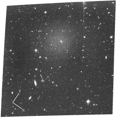
Figure 1: Stacked F814W ACS image of VCC 615, with a total exposure time of 11$\times$1200s. The field of view is 202″$\times$202″, and the Virgo Cluster center (defined by the giant elliptical M87) is 1.95° away (560 kpc in projection) to the east (upper right) of the field.

2.1 Point Source Photometry

Photometry on the ACS images was performed with the ACS module of the DOLPHOT software package (an updated version of HSTPhot; Dolphin, 2000), which is designed for point-source photometry of objects on the individual CTE-corrected flc images using pre-computed Tiny Tim PSFs (Krist, 1995). Object detection and photometry was performed on all 11 F814W images simultaneously, using the deep image stack created above as the astrometric standard (reference) image. We used the most recent version of DOLPHOT 2.0 to pre-process the raw flc images to apply bad-pixel masks and pixel-area masks (acsmask), split the images into the individual WFC1/2 chip images (splitgroups), and to construct an initial background sky map for each chip from each image (calcsky).

Photometry with DOLPHOT is very dependent on the input parameters used (see the excellent discussion in Williams et al., 2014), so we experimented with a number of input parameters, finally settling on values similar to that used in previous deep crowded-field photometric studies (Williams et al., 2014; Shen et al., 2021) and/or suggested values from the DOLPHOT User’s Manual useful for faint, relatively crowded regions of stellar objects such as that exhibited by VCC 615. More specifically, we used RAPER=3.0 pixels, the FITSKY=2 option for determining the sky values from smaller annuli just outside the aperture radius (but within the adopted PSF size RPSF=13 pixels), and adopting FORCE1=1 so that DOLPHOT ’forces’ objects to be fit as stars. The only changes we made to the usual DOLPHOT workflow was the derivation of the aperture corrections on each chip/image. With so few bright stellar objects in our frames, we found the DOLPHOT computed aperture corrections could be dominated by a few brighter non-stellar objects, which resulted in a large spread of $\sim 0.05$ mag in the F814W magnitudes of bright stars on the individual flc images. To improve this, we input our own visually-selected list of 59 stellar objects from which to derive aperture corrections; while this avoided the above issue, it also meant that some frames had very few objects from which to determine the aperture correction, potentially biasing the magnitudes derived from those images only. Indeed, we found that aperture corrections on images with $N<8$ aperture stars used differed by those with more aperture stars by 0.02 mag. Thus the final adopted aperture corrections for each image/chip are (a) DOLPHOT-computed values for those frames with $N>8$ aperture stars, and (b) a fixed value of $-0.038$ (based on the average value from DOLPHOT values from the $N>8$ group) for those frames where $N<8$. This reduced the standard deviation of the individual magnitudes to less than 0.03 mag. We consider this a lower limit on the total absolute error in our final, DOLPHOT-combined F814W magnitudes. Finally, the instrumental magnitudes were converted to the VEGAmag HST photometric system by using a zeropoint of 25.523 for F814W used in the most recent version of DOLPHOT. We report all photometry in Vega magnitudes unless explicitly stated otherwise.

2.1.1 Artificial Stars

We also used DOLPHOT to determine photometric completeness and uncertainty through artificial star tests. We injected 100,000 artificial stars into the ACS image over a magnitude range $22<{\rm F814W}<29$, and use the same cuts on photometric signal-to-noise and image shape (see below) that we use in extracting the actual photometric data. Averaged across the entire ACS field, we find a 50% completeness limit of F814W=27.9, but as seen in Figure 2, the exact value depends somewhat on the distance from the center of VCC 615. Because of the galaxy’s very low surface brightness, the common factors contributing to incompleteness — such as crowding and heightened integrated light — are reduced, such that the radial gradient in incompeteness is rather mild. In empty regions far from VCC 615 (at $R>100$″) 50% completeness is found at F814W=28.1, while in the inner parts of the galaxy (at $R<30$″) the limit has risen by less than half a magnitude, to F814W=27.7. At the average 50% limit of F814W=27.9 the median photometric error as reported by DOLPHOT is $\approx$ 0.18 mag, but Figure 2 shows that the true error (defined as the difference between the injected and measured magnitudes of the artificial stars) shows a complicated behavior: at faint magnitudes the scatter in photometric error becomes asymmetric and biased towards measuring magnitudes slightly fainter than true (by $\sim$ 0.15 mag at F814W=27.9; see also Danieli et al. (2020); Shen et al. (2021)). We fold these biases in photometric skew and scatter as a function of magnitude into our RGB distance estimation in Section 4 below.

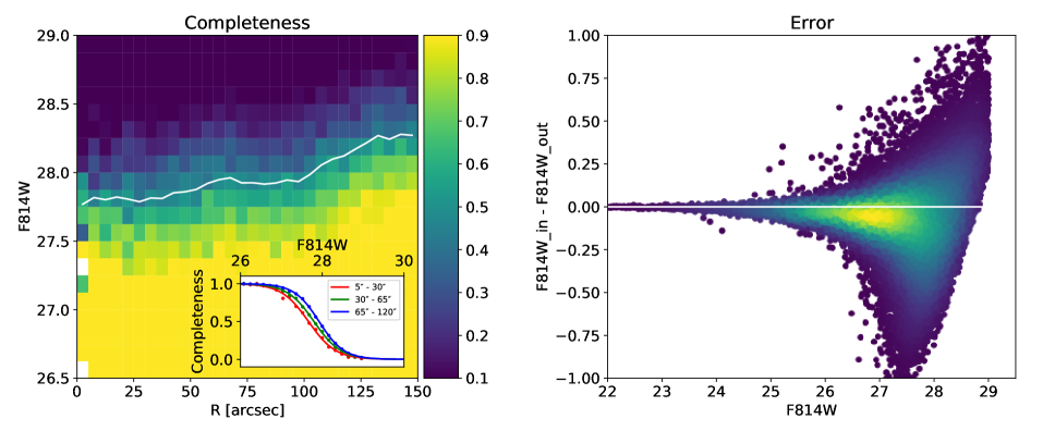
Figure 2: Photometric completeness and uncertainties measured using artificial star tests. The colormap in the left panel shows completeness as a function of magnitude and distance from the center of VCC 615, with the white line showing the 50% completeness limit as a function of radial distance. The inset plot in that panel shows the completeness curves extracted in three different radial ranges.

The right panel shows the absolute error in derived magnitude (i.e., the difference between input and output magnitudes) as a function of magnitude.

2.1.2 Point Source Selection

To assemble the final, cleanest photometric sample of stellar sources on our imaging data, we start by applying a number of photometric and spatial cuts to the DOLPHOT photometry to avoid spurious objects from contaminating the sample; this is particularly important since our deep imaging is only in one filter and thus has no color information to aid in the selection of RGB stars. We begin by removing sources found within 60 pixels of the edge of the stacked F814W image, as well as any source detected near the bright column bleed visible in the northeast (right) side of the images. Next, we mask any source found on or near saturated stars and bright background galaxies on the image — these are typically sources which are either saturated star artifacts or objects intrinsic to the background galaxy, rather than being RGB stars in VCC 615 (or the surrounding Virgo environment). We also only select objects with DOLPHOT object TYPE = 1 (“good star”) and signal-to-noise $>3.0$, which removes obviously extended sources and sources at low $S/N$. To remove sources with suspect photometry due to crowding by nearby objects, we also reject sources with the DOLPHOT CROWD parameter $>0.2$. Finally, we apply a more rigorous cut on the DOLPHOT sharpness parameter to select only those objects most likely to be point sources. Based on visual inspection of objects over a wide range of brightness, we use a selection function of $|{\rm SHARP}|<0.1+0.6e^{\rm F814W-28.7}$, similar in form to our previous studies of stellar populations in the nearby galaxies M81 (Durrell et al., 2010) and M51 (Mihos et al., 2018). When applied to our artificial star tests, this sharpness cut removes only 2.5% of the sources brighter than our 50% completeness limit, demonstrating that this cut is not overly aggressive at removing true point sources. After all cuts, the final photometric sample contains 16,045 sources over the entire ACS field, with 5,023 sources brighter than our 50% completeness limit of F814W=27.9.

3 Spatial Distribution of Point Sources

Figure 3 shows the spatial distribution of the sources in our final photometric catalog over the magnitude range $26.5\leq{\rm F814W}\leq 28.0$. Overall, the radial decline in density around VCC 615 is clear. On small scales, some regions appear devoid of sources; this is due to the presence of bright stars or galaxies in that region, around which we have rejected sources from our catalog. We also note an overdensity of sources near the upper right corner of the image. These sources are embedded within a very diffuse envelope of starlight roughly 4″ in radius (320 pc at Virgo); this object appears to be a small, uncataloged, and extremely low surface brightness dwarf galaxy in which we have resolved its brightest stars. To avoid sources in this object biasing our estimate of the background source density, we mask the object when characterizing populations in the field.

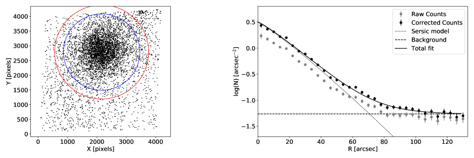
Figure 3: Left: The spatial distribution of detected point sources in our photometric sample over the magnitude range $26.5\leq{\rm F814W}\leq 28.0$. The blue circle shows the 65″radius inside which we draw our photometric sample of VCC 615 stars, while red circle shows the 80″radius outside which we measure background contamination. Right: The radial number density of stellar sources. Grey points show the observed number density, while black points show the profile corrected for radially varying incompleteness. The fitted Sérsic profile is shown as a black line.

Figure 3 also shows the radial density profile of point sources around VCC 615, selected in the same magnitude range shown in Figure 3a. In this plot, grey points show the raw counts, while black points show the corrected profile after applying the radially-dependent incompleteness correction shown in Figure 2. The density profile follows a roughly exponential decline with radius (equivalent to a Sérsic profile with index $n=1$), typical for low luminosity spheroidals in the Virgo Cluster. The density distribution of sources at large distances from VCC 615 show no evidence of clustering in ways that suggest the presence of low density stellar streams or tidal distortions of the galaxy. We confirmed this by smoothing the density field on a variety of spatial scales and looking at the resulting isodensity contours; in no case was any significant structure found beyond a radius of $\sim 70$″. The isodensity contours of the galaxy appear quite round, consistent with the $g$-band isophotal analysis of Lim et al. (2020), who found an axial ratio of ($(b/a)=1$) and no obvious tidal features around the galaxy. Fitting the density profile shown in Figure 3 to a Sérsic model with constant background yields an effective radius of $r_{e}=28.3\arcsec\pm 0.5\arcsec$ and Sérsic index $n=0.88\pm 0.04$. Compared to the $g$-band integrated light profile from NGVS data ($r_{e}=26.33\arcsec$, $n=0.67$, $\langle\mu_{g}\rangle_{e}$=26.86; Lim et al. 2020), our stellar density profile is similar in effective radius but shows a somewhat higher Sérsic index.

The surface density of contaminating sources in the field surrounding VCC 615 is likely due to a combination of unresolved background objects and possible intracluster red giants in the Virgo environment. Over the magnitude range $27\leq F814W\leq 28.5$, the logarithmic slope of the counts in the field is $\approx+0.75\ {\rm dex\ mag^{-1}}$, comparable to that found by Mihos et al. (2018) ($+0.6\ {\rm dex\ mag^{-1}}$) for imaging in the parallel fields of the Abell 2744 Hubble Frontier Field data (Lotz et al., 2017). However the density of sources here is roughly three times higher than that found in the Frontier Field data. Around VCC 615 we find a source density of 0.055 arcsec^-2 over that same magnitude range, compared to 0.0175 arcsec^-2 in the Frontier Field. This difference signals the likely presence of Virgo intracluster stars around VCC 615. While deep imaging of Virgo detects no intracluster light (ICL) in the field down to a limiting surface brightness of $\mu_{B}=29.5$ mag arcsec^-2 (Mihos et al., 2017), star counts are able to trace the ICL even deeper in equivalent surface brightness. We can use the background source level around VCC 615 to place an upper limit on the underlying ICL surface brightness. If we assume all these sources are old (10 Gyr) metal-poor ([M/H]$=-2$) red giants at the Virgo distance, the PARSEC stellar population synthesis models (Bressan et al., 2012) yield an equivalent surface brightness of $\mu_{B}>30.1$ mag arcsec^-2, consistent with the lack of diffuse broadband light around VCC 615 (Mihos et al., 2017). However, the true ICL surface brightness is likely even lower, since many of these sources will be true background objects rather than intracluster stars. If true background objects are present at a level comparable to that traced by the Frontier Field data, subtracting that level from the observed number density yields our best estimate for local surface brightness of the Virgo ICL around VCC 615: $\mu_{B}=30.5$ mag arcsec^-2.

The spatial distribution of sources in the field also lets us determine the optimal radial range for our TRGB analysis. Choosing a smaller radius will reduce background contamination but yield fewer stars for the photometric sample, while a larger radius will contain more stars but also make contamination worse. Given the surface density profile fits shown in Figure 3b, we choose an outer radius for the galaxy of $65\arcsec$; enlarging the radius beyond this value adds background contaminants at a faster rate than VCC 615 stars. The luminosity function of sources within VCC 615 (i.e., at $r\leq 65\arcsec$) is shown in Figure 4, as is the luminosity function of the background sources measured at $r>80\arcsec$, where the density profile shown in Figure 3 levels off to a constant background density. The contamination fraction, defined as the ratio of the surface density of counts in the background to that within VCC 615, is shown in the bottom of the figure, and is $\approx$ 0.1–0.2 over the magnitude range $26.5\leq{\rm F814W}\leq 28.0$, climbing to values $\gtrsim 0.5$ at magnitudes fainter than F814W=28.5.

In the VCC 615 luminosity function, the counts show a relatively shallow slope at fainter magnitudes, but drop off much more quickly at magnitudes brighter than F814W $\approx$ 27.3, likely marking the approximate RGB tip. However, even brighter than the tip we find an excess of stellar sources in VCC 615, suggesting the presence of asymptotic giant branch (AGB) stars indicative of an intermediate age population.

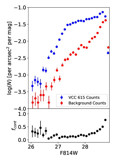
Figure 4: Top: The observed, binned luminosity function of stellar sources in VCC 615 and the surrounding field (uncorrected for incompleteness). Bottom: The estimated contamination fraction of background sources in the VCC 615 luminosity function, defined as $N_{back}/N_{VCC615}$.

3.1 The nearby LSB dwarf galaxy

Before turning to the TRGB analysis of VCC 615, we return briefly to the dwarf galaxy detected near the upper right (east) edge of our ACS field, at a position of $(\alpha,\delta)_{J2000.0}=$ (12:23:11.0, +12:01:10.3). Figure 5 shows the ACS imaging of this object in more detail, along with deep $g$-band imaging of the field from NGVS, where the object is also clearly visible. The luminosity function of point sources detected within the 4″ is shown in Figure 6; while the total number of sources detected (55) is too small to do robust modeling of the luminosity function, the shape of the distribution is consistent with what one would expect for RGB stars at the distance of Virgo: a jump in counts near the expected RGB tip at F814W $\approx$ 27, with a steep rise towards fainter magnitudes. If we assume the object is at the Virgo distance of 16.5 Mpc, then after correction for contamination and incompleteness, inside the $r=4\arcsec$ circle shown in Figure 5 we find $N=12^{+2}_{-1}$ sources between $m_{tip}$ and $m_{tip}+0.5$. Assuming an old (10 Gyr) metal-poor ([M/H]=$-1.5$) stellar population as described by the PARSEC models of Bressan et al. (2012), these counts would correspond to a total stellar mass (inside of the 4″ radius) of $6.8^{+1.2}_{-0.7}\times 10^{5}\ {\rm M_{\sun}}$ and a $g$-band magnitude of $m_{g}=23.0^{+0.1}_{-0.2}$.

While the object is clearly detected in the deep NGVS $g$-band imaging, its small size, low surface brightness, and proximity to a nearby bright ($g=12.3$) star makes detailed surface photometry difficult. Rather than do a full Sérsic model of the light profile, we instead fit a simple exponential model to the profile (i.e., Sérsic $n=1$, typical of low luminsity spheroids in Virgo), yielding $r_{e}=5.1\pm 0.3\arcsec$, $\langle\mu_{g}\rangle_{e}=27.4\pm 0.1$ mag arcsec^-2, and $m_{g,tot}=21.8\pm 0.1$. This total magnitude is nearly identical to the 50% completeness limit of the NGVS Virgo galaxy catalog ($m_{g,50}=22.0$ Ferrarese et al., 2020); that and the contamination from the nearby star explain its absence in the NGVS catalog. Inside $r=4\arcsec$, the object has an integrated magnitude of $m_{g}=22.9$, comparable to that derived above using counts near the RGB tip. At the Virgo distance, these numbers translate to an absolute $g$ magnitude of $M_{g}=-9.2$ and a physical effective radius of $r_{e}=400$ pc, roughly similar to Milky Way dwarf spheroidals such as Sextans or Ursa Minor (e.g.,  McConnachie, 2012). Whether or not this object is physically associated with VCC 615 is unclear; while it is projected only 90″ (7.2 kpc) away, we see no evidence for interaction between the two, and it may just be a chance projection in the crowded Virgo Cluster environment.

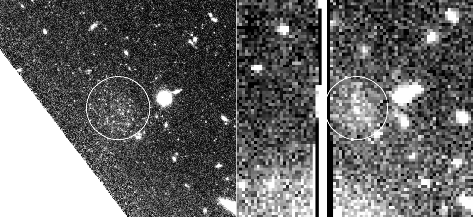
Figure 5: Virgo dwarf galaxy candidate imaged in our ACS data (left) and in deep NGVS $g$-band imaging (right). North is up, East is to the left, and the circle has a radius of 4″. The NGVS image has been rebinned 2x2 pixels to increase signal to noise, and the vertical column bleed and scattered light at the bottom of that image are both due to a bright ($g=12.3$) star 30″ to the South.

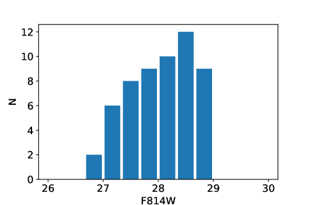
Figure 6: The luminosity function of point sources detected within 4″ of the dwarf galaxy candidate shown in Figure 5, in bins of width $\Delta m=0.33$ mags.

4 TRGB Distance Estimation

In principle, the sharpness of the luminosity function discontinuity at the RGB tip means that “edge detectors” such as the classical Sobel filter can detect it in a straightforward fashion (see, e.g.,  Sakai et al., 1996; Madore et al., 2009; Jang & Lee, 2017; Beaton et al., 2018). In our case, however, a number of factors complicate such an approach. We have potentially significant contamination in our sample, due both to the likely presence of intracluster red giant stars and to the fact that, working in only one filter, we have no color information to help remove background contaminants. Furthermore, we are working near the limiting depth of the data, where the completeness corrections and asymmetric photometric errors begin to play important roles in the error distributions. The combination of these effects means that any discrete break in the underlying luminosity function ends up being both diluted and smeared asymmetrically, and becomes very hard to find using classical edge-detector algorithms.

To derive the red giant branch tip magnitude in VCC 615, we instead use a Bayesian approach similar to that used in previous TRGB studies of old stellar populations in nearby galaxies (e.g., Makarov et al. 2006; Tollerud et al. 2016). In this approach, we model the underlying stellar luminosity function, convolved with the photometric errors and incompleteness derived from our artificial star tests, and with background contamination added based on the LF of sources in the surrounding environment. This model involves five free parameters (described below) along with strongly non-Gaussian photometric errors, making a Bayesian approach ideal for parameter extraction. This approach also factors in the photometric data all along the luminosity function, not just at the location of the break, making it a more robust measure of behavior of the luminosity function as it crosses the RGB tip.

For the underlying stellar luminosity function (before errors or contamination), we adopt a broken power law form:

$$\psi(m)=\begin{cases}10^{a(m-m_{\rm tip})+b},&m>m_{\rm tip}\\ 10^{c(m-m_{\rm tip})},&m<m_{\rm tip}\end{cases}$$ (1)

where $m_{\rm tip}$ is the magnitude of the RGB tip, $a$ and $c$ are the power law slopes of the luminosity function fainter and brighter than the RGB tip, respectively, and $b$ is the discontinuity in counts at the tip. Choices for these parameters are described in more detail below.

For a given input luminosity function, we then factor in photometric errors, incompleteness, and contamination to create an observed luminosity function:

$$\phi(m)=\int\psi(m^{\prime})C(m^{\prime})E(m^{\prime})dm^{\prime}+B(m),$$

where $C$ and $E$ are the photometric incompleteness and uncertainty models, respectively, and $B(m)$ is the background contamination model, all described below.

We model the incompleteness using the logistic function:

$$C(m)={1\over{1+e^{(m-m_{50})/w}}}$$

where $m_{50}$ is the 50% completeness limit and $w$ describes how quickly the completeness drops around $m_{50}$. For simplicity, we do not incorporate a spatially varying incompleteness model, but rather use a single function where the parameters of the logistic function are derived from artificial stars located over the same radial range from which we draw the observed VCC 615 luminosity function ($r=5-65\arcsec$), yielding $(m_{50},w)=(27.77,0.33)$.

The photometric error model is more complicated. An examination of Figure 2b shows that there is both a systematic shift and asymmetric spread of the photometric error as a function of magnitude, and is not well-described by a simple Gaussian model. Instead, we use a skew-normal distribution (Azzalini & Capitanio, 1999) to model the error function:

$$E(m)=\left({2\over w}\right)G\left({{m-m_{0}}\over\omega}\right)F\left(\alpha{{m-m_{0}}\over\omega}\right),$$

where $G$ is a normal Gaussian function and $F$ is its cumulative distribution function. The parameters $m_{0},\omega,$ and $\alpha$ describe the offset, spread, and asymmetry of the skew-normal distribution, respectively. We bin the artificial stars by magnitude, using bins of 0.2 mag width, then fit $m_{0},\omega,$ and $\alpha$ as a function of magnitude to capture the change in shift and asymmetry as a function of magnitude.

Finally, we model background contamination as $B(m)=f_{c}\times\rho_{b}(m)$ where $\rho_{b}$ is the luminosity function of the background area shown in Figure 4 and $f_{c}$ is the ratio of the background counts to total counts measured at F814W=28.0. Based on the luminosity functions shown in Figure 4, $f_{c}=0.18$, but in our Bayesian analysis we allow it to vary somewhat to capture the uncertainty in the overall normalization of the background luminosity function. We note that unlike the parameterized stellar luminosity function $\psi$, the background luminosity function comes directly from the imaging data, so we need not apply the error and incompleteness models to it — these effects are implicitly contained in the derived background luminosity function.

Given a model luminosity function, the log likelihood function is then given by (Makarov et al., 2006):

$$\mathcal{L}=-\sum_{i=1}^{N}\ln\phi(m_{i}|\mathbf{x})+N\ln\int_{m_{\rm min}}^{m_{\rm max}}\phi(m|\mathbf{x})dm$$

where x represents the five parameters of the model ($m_{\rm tip},a,b,c,$ and $f_{c}$) and the summation is over every star detected in the magnitude range $(m_{\rm min},m_{\rm max})$. We restrict our analysis to the magnitude range F814W=(26,28); at brighter magnitudes there are very few sources, while at fainter magnitudes both incompleteness and contamination begin to dominate the photometry. Our priors on the different parameters are set by a variety of considerations. For the RGB tip magnitude we use a uniform prior over the range F814W=26.5–27.5 (i.e., $m_{\rm tip}=U(26.5,27.5)$); the rapid decline in counts brighter than F814W $\approx$ 27 suggests this is the approximate location of the tip, and this is also the expected tip magnitude for old stellar populations roughly at the distance of the Virgo Cluster. To assign the prior on the slope of the luminosity function fainter than the tip, we rely on studies of the RGB slope in nearby galaxies (Méndez et al., 2002; Makarov et al., 2006) which generally find a logarithmic slope of 0.3, and hence adopt a Gaussian prior on the RGB slope of $a=G(0.3,0.1)$. For the background contamination fraction, we use our direct measure of contamination on the image ($f_{c}=0.18$), and adopt a Gaussian prior of $f_{c}=G(0.18,0.1)$ to allow for some variation due to spatial inhomogeneity in the background counts. The slope of the counts brighter than the RGB tip is a bit more problematic; these objects could arise from a variety of sources with ill-constrained luminosity functions, such as AGB stars, chance blends, and uncorrected contamination. For this portion of the luminosity function we allow a wide uniform prior on the slope of $c=U(0,2)$. Finally, for the discontinuity across the RGB tip (the “break strength”) we assign another wide uniform prior of $b=U(0,1)$.

To estimate the RGB tip magnitude we use the Markov Chain Monte Carlo code emcee v3 (Foreman-Mackey et al., 2019) to sample parameter space for the modeled luminosity function and marginalize over the remaining parameters. We initialize the walkers using the prior distributions for the parameters, burn in the sampler for 1500 samples ($\approx$ 20 autocorrelation times), and then run an additional 5000 samples for the final analysis, the results of which are summarized in Figure 7. During this analysis, we adopt a foreground extinction correction of $A_{\rm F814W}=0.04$ (Schlafly & Finkbeiner, 2011), and the RGB tip magnitudes reported below include that extinction correction.

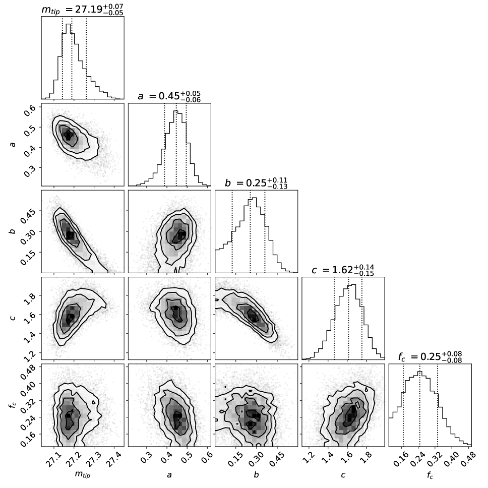
Figure 7: Posterior probability density profiles for the model luminosity function parameters: TRGB magnitude ($m_{\rm tip}$), luminosity function slope below the tip ($a$), TRGB break strength ($b$), bright end luminosity function slope ($c$), and background contamination fraction ($f_{c}$). Dotted lines show the median and 16th/84th percentiles of the marginalized distributions.

Marginalized over the other parameters, our final estimate for the TRGB is $m_{\rm tip,F814W}=27.19_{-0.05}^{+0.07}$, where the error bars refer to the 84th/16th percentiles of the distribution. The posterior distribution on $m_{\rm tip}$ shows a clear peak, but with an asymmetric tail towards fainter values. An examination of the covariances between the parameters in Figure 7 shows that this tail is due to models with weaker break strengths (lower values for $b$) and steeper slopes for the bright end of the luminosity function (larger values for $c$).

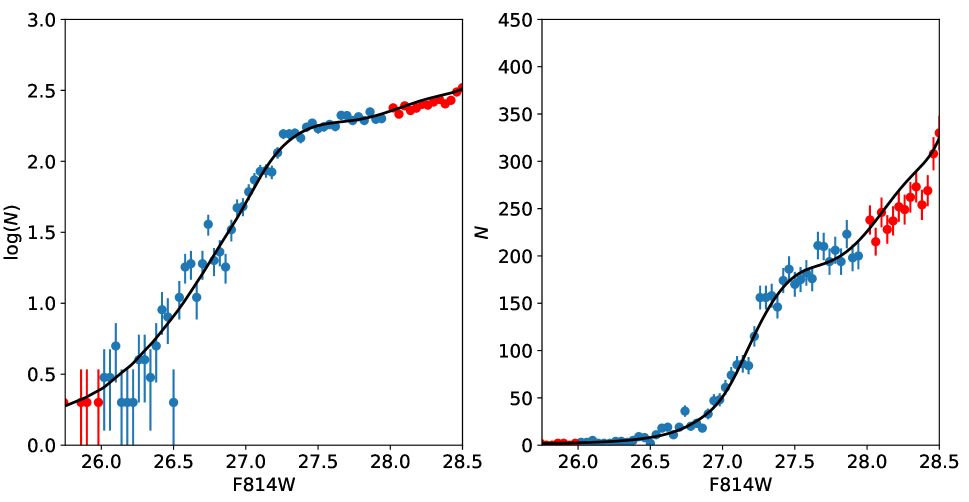
Figure 8: The best fit luminosity function model (black line) overlaid on the binned observed luminosity function. Red points show magnitude ranges excluded from the MCMC analysis.

We also examine how our results depend on the radial range chosen for the analysis. In principle, this choice could lead to systematic differences in the derived TRGB, for a variety of reasons, including stellar population gradients within VCC 615 or an increased contamination fraction in the galaxy’s low density outskirts. We break the detected point sources within VCC 615 into two radially separate samples: an inner sample covering $r=$ 5″–30″ and an outer sample at $r=$ 30″–65″, with each having roughly similar numbers of stars. We then run the analysis on each sample separately to look for systematic differences in the derived parameters of the underlying luminosity function. These results are shown in Table 1.

Comparing the inner and outer samples, we see a slight change in the inferred RGB tip magnitude of $\Delta m_{\rm tip}=0.1$, albeit only at the $1\sigma$ level. If real, this difference may hint at a slight metallicity gradient in the galaxy – while the absolute magnitude of the RGB tip in F814W is relatively constant at metallicities lower than $[M/H]=-0.7$ (Serenelli et al., 2017; Beaton et al., 2018), models suggest slight systematic trends between $M_{\rm tip}$ and $[M/H]$ may still be present at the 0.1 mag level. The general trend is for the tip magnitude to become fainter as metallicity increases (e.g.,  Rizzi et al., 2007; Serenelli et al., 2017; Jang & Lee, 2017), a more metal-poor outer disk would thus show a slightly brighter tip magnitude, like that suggested by our analysis. But at even lower metallicity ($[M/H]<-1$), models suggest this trend may reverse, with the tip magnitude becoming fainter as metallicity continues to decrease. Given its low luminosity, VCC 615 likely is quite metal-poor; placing it on the luminosity-metallicity relationship (Skillman et al., 1989; Grebel et al., 2003; Kirby et al., 2013), suggests it has a metallicity near $[M/H]\approx-1$, but without a firm estimate of its metallicity, and given the uncertainties in both the models and the data, we leave any intrinsic metallicity gradient as a possible systematic for further study.

However, another plausible explanation for the slight difference in the inferred tip magnitude between the inner and outer samples is the effect of contamination from intracluster RGB stars within the Virgo Cluster itself. Our inferred tip magnitude ($m_{\rm tip}=27.19$, derived from the full sample) places VCC 615 slightly behind the cluster core. A population of intracluster stars concentrated in the Virgo Core would act as foreground contaminants with slightly brighter tip magnitude. Since the fractional contamination would be worse in the outskirts of VCC 615, where the galaxy’s stellar density is lower, such contamination would manifest as the outskirts having a systematically brighter tip magnitude and higher inferred contamination fraction compared to the inner sample of stars, precisely as seen in Table 1.

Finally, we also look at the systematic effects of extending the analysis to fainter magnitude ranges, down to F814W=28.3 or 28.5. At these magnitudes, the stellar incompleteness fraction is high (only 20% (12%) of stars at F814W$=28.3\ (28.5)$ are recovered in our artificial star tests), and the counts start to become dominated by background contaminants (see Figure 4). However, this gives us an opportunity to better constrain how background contamination may be diluting and influencing the derived tip magnitude, and also explore any systematic behavior between the estimated contamination fraction and other inferred parameters of the fitted luminosity function. The results of this analysis are also shown in Table 1, where it can be seen that the derived tip magnitude has little dependency on the magnitude range of the analysis. Extending the analysis to fainter magnitudes does lead to slight increases in the derived contamination fraction ($f_{c}$), but this comes with a corresponding decrease in the inferred RGB slope (lower values for $a$). In essence, at faint magnitudes, the MCMC analysis is trading off steeper RGB slopes for a higher contamination fraction, but with little impact on the parameters at the brighter end of the luminosity function. Given the low stellar completeness and the uncertainties in the background contamination, we do not consider these degenerate shifts in the faint end parameters of the luminosity function to be meaningful.

In summary, these various tests show that the derived luminosity function parameters (and most importantly the RGB tip magnitude, $m_{\rm tip}$) are not highly sensitive to the radial or magnitude range of the photometric sample being analysed. While there is some hint that factors such as metallicity or contamination from intracluster RGB stars may possibly affect our estimate of $m_{tip}$, the evidence is weak, only at the $1\sigma$ level. Without additional information to constrain the metallicity of the stellar population or the presence of intracluster RGB stars, we simply leave this as an open systematic and use the tip magnitude of $m_{\rm tip}=27.19^{+0.07}_{-0.05}$ (estimated over the range $r=5\arcsec$–$65\arcsec$ and $F814W=26.0$–$28.0$) as our best estimate of the RGB tip magnitude in VCC 615. Adopting the Freedman et al. (2020) calibration of the absolute magnitude of the RGB tip ($M_{\rm tip,F814W}=-4.054\pm 0.022\ \rm{(stat)}\pm 0.039\ \rm{(sys)}$) for old metal-poor stellar populations, we derive a final distance estimate of $d=17.7^{+0.6}_{-0.4}$ Mpc, where the uncertainties include the statistical uncertainty in $M_{\rm tip,F814W}$. This distance places VCC 615 slightly behind the Virgo core, at a distance of $d_{\rm Virgo}=16.5\pm 0.1$ Mpc (; ).

The second, complementary comparison of VCC 615’s location with respect to the Virgo core comes from comparing our VCC 615 TRGB estimate to that for intracluster stars in the Virgo core by Lee & Jang (2016), based on observations by Williams et al. (2007). Lee & Jang (2016) find a RGB tip magnitude of $m_{\rm tip,I}=26.93\pm 0.03$. Including the small $-0.007$ magnitude correction to convert $I$ to F814W (Freedman et al., 2019), we get a difference in the F814W tip magnitudes of $\Delta m=m_{\rm tip,VCC615}-m_{\rm tip,Virgo}=+0.33\pm 0.07$, or a relative distance ratio of $d_{\rm VCC615}/d_{\rm Virgo}=1.17\pm 0.04$, again putting VCC 615 on the far side of Virgo.

As one final consistency check on the nature of the sources in our VCC 615, we also calculate the ratio of detected stellar sources to the total broadband light and compare to the expectation from stellar population synthesis models. Within a radius of $r=50\arcsec$, we measure a total of $N_{*}=2380$ RGB stars between $m_{tip}$ and $m_{\rm tip}+0.5$, after correcting for spatial incompleteness, photometric incompleteness, and background contamination. Using the $g$-band integrated light profile from NGVS data ($r_{e}=26.33\arcsec$, $n=0.67$, $\langle\mu_{g}\rangle_{e}$=26.86; Lim et al. 2020), and adopting our TRGB distance of 17.7 Mpc, this gives a ratio of $N_{*}/L_{g,\sun}=5.7\times 10^{-5}$ within $r=50\arcsec$. The PARSEC population synthesis models of Bressan et al. (2012) predict values in the range $N_{*}/L_{g,\sun}=5.5-7\times 10^{-5}$, for populations spanning a range of metallicities $[M/H]=-0.7$ to $-2$ and ages 6 to 10 Gyr, in good agreement with our measured value.

Table 1: MCMC Modeling Results

Region	Radial Range	$N_{*}$	$m_{\rm tip}$	$a$	$b$	$c$	$f_{c}$
Magnitude Range: 26.0 – 28.0
All	5″–65″	4177	$\bf 27.19^{+0.07}_{-0.05}$	$\bf 0.45^{+0.05}_{-0.06}$	$\bf 0.26^{+0.11}_{-0.13}$	$\bf 1.62^{+0.14}_{-0.15}$	$\bf 0.25^{+0.09}_{-0.08}$
Inner	5″–30″	2179	$27.27^{+0.09}_{-0.08}$	$0.42^{+0.07}_{-0.08}$	$0.18^{+0.13}_{-0.12}$	$1.64^{+0.12}_{-0.13}$	$0.20^{+0.08}_{-0.06}$
Outer	30″–65″	1998	$27.17^{+0.09}_{-0.06}$	$0.43^{+0.07}_{-0.07}$	$0.32^{+0.16}_{-0.18}$	$1.60^{+0.20}_{-0.24}$	$0.32^{+0.09}_{-0.09}$
Magnitude Range: 26.0 – 28.3
All	5″–65″	5941	$27.20^{+0.07}_{-0.04}$	$0.38^{+0.04}_{-0.05}$	$0.25^{+0.11}_{-0.13}$	$1.64^{+0.13}_{-0.15}$	$0.29^{+0.08}_{-0.08}$
Inner	5″–30″	3002	$27.28^{+0.08}_{-0.07}$	$0.37^{+0.05}_{-0.06}$	$0.19^{+0.13}_{-0.13}$	$1.63^{+0.12}_{-0.13}$	$0.21^{+0.08}_{-0.07}$
Outer	30″–65″	2939	$27.16^{+0.07}_{-0.05}$	$0.43^{+0.05}_{-0.06}$	$0.33^{+0.15}_{-0.17}$	$1.59^{+0.21}_{-0.24}$	$0.36^{+0.08}_{-0.09}$
Magnitude Range: 26.0 – 28.5
All	5″–65″	7261	$27.24^{+0.08}_{-0.05}$	$0.32^{+0.04}_{-0.05}$	$0.21^{+0.12}_{-0.13}$	$1.67^{+0.11}_{-0.13}$	$0.33^{+0.05}_{-0.05}$
Inner	5″–30″	3588	$27.30^{+0.08}_{-0.07}$	$0.32^{+0.06}_{-0.06}$	$0.17^{+0.13}_{-0.11}$	$1.66^{+0.11}_{-0.11}$	$0.26^{+0.06}_{-0.06}$
Outer	30″–65″	3673	$27.18^{+0.09}_{-0.06}$	$0.38^{+0.05}_{-0.06}$	$0.31^{+0.16}_{-0.18}$	$1.62^{+0.19}_{-0.24}$	$0.37^{+0.06}_{-0.06}$

Note. — The marginalized parameters of the VCC 615 RGB luminosity function derived for photometric samples with differing radial ranges and magnitude ranges. $N_{*}$ shows the number of objects in each sample. $m_{\rm tip}$ is the F814W magnitude of the RGB tip, $a$ and $c$ are the logarithmic slope of the LF fainter and brighter than the tip magnitude, respectively, $c$ is the logarithmic discontinuity in counts at the tip, and $f_{c}$ is the contamination fraction measured at F814W=28.0. Error bars in the derived parameters show the 16th/84th percentile ranges.. Our adopted model solution is shown in boldface. See text for details.

5 Discussion

With a best fit TRGB distance to VCC 615 of $d=17.7^{+0.6}_{-0.4}$ Mpc, our analysis places the galaxy $1.2^{+0.6}_{-0.5}$ Mpc on the far side of the Virgo Cluster. Its three dimensional position relative to M87 gives it a Virgocentric radius of $\approx 1.3$ Mpc, close to the cluster’s virial radius ($R_{200}=1.5$ Mpc; McLaughlin 1999). This placement of VCC 615 on the far side of Virgo is also supported by its fainter RGB tip magnitude compared to intracluster red giants measured by Lee & Jang (2016), and any weak systematic effects we could plausibly identify in our analysis would push the galaxy even further beyond the Virgo core. The galaxy’s measured line-of-sight velocity ($v_{\rm VCC615}=2094\pm 3$ km s^-1; Toloba et al. 2018) is redshifted by $\approx$ 1000 km s^-1compared to the Virgo mean velocity ($v_{\rm Virgo}=1088\pm 105$ km s^-1; M07). Projecting the relative line of sight velocity onto the Virgo radius vector gives a radial velocity with respect to the cluster of $875\pm 140$ km s^-1, where the uncertainty reflects both the VCC 615 distance uncertainty and the uncertainty in the cluster mean distance and velocity. Of course, the unknown velocity in the sky plane will affect Virgocentric radial velocity as well, but since the largest component of the radius vector is along our line of sight, the true Virgocentric radial velocity is unlikely to be much different from that calculated here.

While VCC 615’s radial velocity is somewhat high for Virgo cluster member galaxies, it is not anomalously so. At the galaxy’s position within Virgo, the escape velocity from the main cluster (using the mass model of McLaughlin 1999) is $\approx$ 2400 km s^-1. Unless the unknown transverse velocity is significantly higher than the galaxy’s Virgocentric radial velocity of 875 km s^-1, VCC 615 is thus likely a bound member of the Virgo cluster. Figure 9 places VCC 615 on the distance-velocity diagram for other Virgo galaxies determined using surface brightness fluctuation distances from B09. Galaxies within Virgo have a large velocity spread; the main cluster (Virgo A) has a velocity dispersion of $\sigma_{v_{r}}=593\pm 68$ (Mei et al., 2007), but the full velocity range is much higher: $-220\ {\rm km\ s^{-1}}\leq v_{r}\leq+2300\ {\rm km\ s^{-1}}$ (see also Binggeli, Tammann, & Sandage, 1987). In Figure 9, VCC 615 follows the general distribution of other Virgo galaxies, and we also see no evidence for VCC 615 being part of any of Virgo’s kinematically distinct substructure. Projected 1.9° WSW of M87, the galaxy does not lie within any of the boundaries of the Virgo M, W^′ or W clouds (as defined by Binggeli, Tammann, & Sandage 1987), nor is its distance or radial velocity consistent with those subgroups.

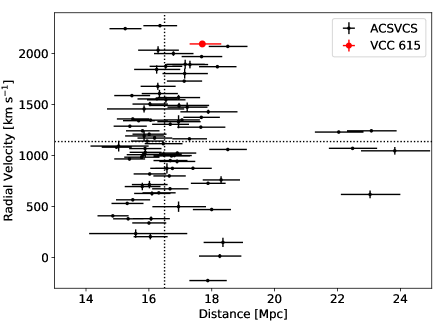
Figure 9: Velocity-distance plot for galaxies in Virgo. Black points are galaxies from the ACS Virgo Cluster Survey, with distances derived from surface brightness fluctuations (; ). The red point shows our TRGB distance to VCC 615, along with its measured radial velocity from Toloba et al. (2018). Grey dotted lines show the mean Virgo distance (16.5 Mpc) and velocity (1138 km s^-1) from ; .

Thus the combined position-velocity data for VCC 615 are consistent with the galaxy being a kinematically normal member of the main Virgo cluster. Furthermore, the galaxy is currently on an outbound trajectory, leaving the inner parts of the cluster. Under the simplest assumption of a free-flight line-of-sight trajectory (i.e., no transverse velocity), the galaxy would have experienced Virgo pericenter 1.3 Gyr ago, having passed 0.5 Mpc from the cluster center. Of course, since a free-flight calculation disregards the effects of the cluster potential, it overestimates the time since periapse passage. Nonetheless, it is clear that VCC 615 is not on an inbound trajectory, and if it is an object that recently fell into the cluster for the first time, it has had many dynamical times to respond to the effects of the cluster potential. Given the galaxy’s half-light radius (2.2 kpc) and the velocity dispersion of its globular clusters ($\sigma_{v}=32^{+17}_{-10}$ km s^-1; Toloba et al. 2018), the galaxy has a rough dynamical time of $(G\rho)^{-1/2}\approx 70$ Myr, much larger than the crossing time of the cluster.

Without knowing VCC 615’s transverse velocity, it is difficult to make any more definitive statement about its orbital trajectory through Virgo, but with some assumptions about the cluster potential and kinematics, we can make probablistic statements about the dynamical history of the galaxy. To do this, we adopt the NFW mass model of McLaughlin (1999) for Virgo Subcluster A (the main mass component of Virgo), which, scaled to a distance of 16.5 Mpc has the parameters $R_{200}=1.55$ Mpc, $R_{s}=0.62$ Mpc, and $M_{200}=4.2\times 10^{14}M_{\odot}$. Given VCC 615’s three-dimensional position relative to M87 (which we take to define the cluster center), we then assume orbital isotropy, calculate the 1-d velocity dispersion of the NFW profile at that radius (Lokas & Mamon, 2001), and draw the two missing components of VCC 615’s velocity vector from a Gaussian probability distribution given that dispersion. We then use the software package gala (Price-Whelan et al., 2017) to integrate the orbit backwards in the model potential to derive the distance and time of last pericenter passage ($R_{\rm peri}$, $t_{\rm peri}$). We do this for 10,000 randomly sampled trajectories initialized in this fashion to study a plausible distribution of $R_{\rm peri}$ and $t_{\rm peri}$ for VCC 615.

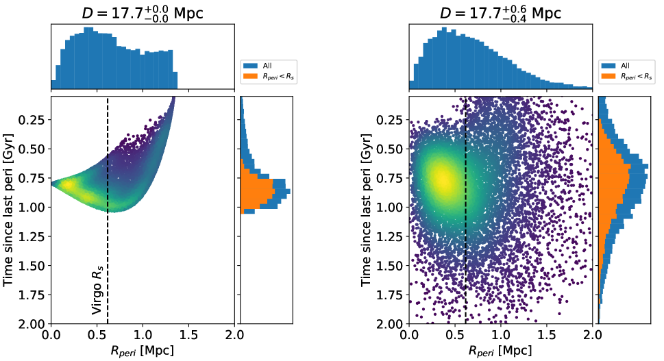
Figure 10: Inferred probablistic orbit distribution for VCC 615, showing the distribution of time and distance of the most recent Virgocentric periapse for orbits which sample a range of tangential motions drawn from the Virgo kinematic model described in the text. The left panel shows orbits which start with VCC 615 precisely at our best-match distance and assuming no uncertainty in the adopted Virgo distance and mean radial velocity. The right panel repeats the analysis, but starts VCC 615 at a range of distances randomly sampled from our uncertainty estimates, and also incorporated the uncertainties in the Virgo distance and velocity. In the main plot, the colormap shows the density of points, while in the histograms, the orange histogram shows the distribution of periapse time for orbits that reach inside the Virgo Cluster scale radius. See text for full details.

The results of this calculation are shown in Figure 10. The left panel shows the results for an ensemble of orbits which all start precisely at our best match distance of $D=17.7$ Mpc and presume no uncertainties on the distance and mean velocity of the cluster. While this makes for an overly idealized calculation, it is instructive for understanding the orbital behavior of the models. Purely radial orbits are those with $R_{\rm peri}$=0, passing through the cluster center $\approx$ 800 Myr ago. At the other extreme are orbits which maximize the tangential velocity; these are now at closest approach ($t_{\rm peri}$=0) and have high velocity across the plane of the sky that is starting to carry them away from pericenter. Between those extremes, at a given $R_{peri}$, orbits with the most recent pericenter passage have high space motion and carry the galaxy quickly through the cluster on orbits that extend well outside $R_{200}$, while orbits with older pericenter times are more tightly bound, with the galaxy moving more slowly, with little transverse space motion. The dashed vertical line in Figure 10 shows the scale radius for McLaughlin (1999) NFW model describing the main body of Virgo(Virgo A; $R_{s}=0.62$ Mpc), used here as a metric defining the cluster core. Half (49.9%) of the orbits in the ensemble travel inside $R_{s}$, with pericenter passages typically happening $\approx$ 750 – 900 Myr ago. While many orbits carry the galaxy inside $R_{s}$, few orbits pass truly deep into the cluster core; only 10.1% of the orbits reach a pericenter closer than 200 kpc of the cluster center.

The right panel of Figure 10 more accurately captures uncertainties in the orbital parameters, by factoring in the uncertainty in VCC 615’s distance, as well as in the Virgo distance and velocity, when initializing the orbits. To capture the velocity uncertainty we start the orbits with a line-of-sight velocity for VCC 615 drawn from a Gaussian with mean $\Delta v=v_{\rm VCC615}-v_{\rm Virgo}$ and dispersion equal to the uncertainty in the Virgo mean velocity ($\pm 105$ km s^-1, Mei et al. (2007)). The uncertainty in position is modeled by sampling the posterior distribution function for our TRGB distance shown in Figure 7. These variations smear out the derived orbital parameters, but the fraction of orbits where the galaxy passes inside $R_{s}$ (49.3%) or inside 200 kpc (9.4%) are both essentially unchanged. The time since pericenter passage for these orbits peaks around 750 Myr, but shows a large distribution, with the 25th and 75th percentile range covering the range 640$-$1030 Myr. Of course, even this statistical analysis of orbits contains a number of dynamical assumptions embedded in it: that the missing components of the tangential velocity can be modeled using the NFW distribution for the Virgo potential; that VCC 615 has not experienced strong interactions with other galaxies in Virgo; and that the influence of other Virgo mass components (such as the Virgo B clump to the south) is negligible. Nonetheless, the broad implications seem robust: VCC 615 is on an outbound trajectory from Virgo, having experienced pericenter passage at least 500 Myr or more in the past.

VCC 615’s outbound orbit shows that rather than being fragile objects relegated to the cluster outskirts, at least some cluster UDGs can and do survive passages through the dense cluster environment. While the uncertainties in the orbit modeling make it ill-advised to project the orbit too far back in time, the galaxy has likely experienced some amount of dynamical processing by the cluster potential; nearly 50% of the orbit projections have it at or inside the cluster core within the past 1.5 Gyr. However, given the VCC 615’s dynamical mass and mass-to-light ratio ($M_{\rm dyn}=2.7\times 10^{9}M_{\odot},(M/L)_{V}=56M_{\odot}/L_{\odot}$; Toloba et al. 2018, both measured inside the globular cluster half light radius, and also scaled for our updated distance), the galaxy is likely quite resilient against the cluster tidal field. At its current Virgocentric distance ($R_{\rm Virgo}=1.3$ Mpc), VCC 615’s tidal radius ($r_{t}=R_{\rm Virgo}(M_{\rm VCC615}/M_{\rm Virgo})^{1/3}$) is $\sim$ 15 kpc, and even within the cluster core the tidal radius remains significantly higher than the galaxy’s effective radius (2.2 kpc). To suffer serious tidal disruption, VCC 615 would need to pass quite close to the cluster center ($\lesssim$ 200 kpc), and our orbit modeling suggests that passages this close are unlikely.

Of course, the Toloba et al. (2018) mass estimate, based on its globular cluster kinematics, presumes that the globulars are fair kinematic tracers of the VCC 615’s dynamical mass. While the galaxy is currently in the outskirts of the cluster where tides should not strongly influence the globular cluster kinematics, a recent core passage could have dynamically heated the clusters and yield an inflated measure of the galaxy’s mass. For example, if the mass-to-light ratio of the galaxy was more similar to that of normal Virgo dE’s ($M/L_{V}\sim$ 3–5, Toloba et al. 2014), its binding mass would be reduced by an order of magnitude. In this case, inside of $R_{s}$ the galaxy’s tidal radius would be reduced to 5 kpc or less, comparable to its effective radius. Thus, in principle, a close core passage could have dynamically heated the galaxy, leading to both its diffuse nature and the high velocity dispersion of its globular cluster system. However, VCC 615 shows no morphological sign of tidal heating — it does not appear tidally distorted, nor do we see any evidence for stellar tidal streams in the galaxy’s outskirts. Thus, while the orbital modeling indicates that an recent core passage for VCC 615 is quite possible, we think it unlikely that such an event has strongly affected the galaxy’s structure or kinematics.

In the context of cluster UDG evolution models, the properties of VCC 615 seem in many ways consistent with the “born-UDG” galaxy populations in the simulations of Sales et al. (2020). In these simulations born-UDGs form as normal LSB galaxies in the field and are later accreted into the cluster, in contrast to “tidal-UDGs” which fell into the cluster early and have been dynamically heated and stripped by the cluster tidal field. Born-UDGs tend to be found in the cluster outskirts, like VCC 615, and have don’t show evidence for suppressed velocity dispersions indicative of significant tidal mass loss. VCC 615’s high velocity dispersion (Toloba et al., 2018) and lack of tidal deformation are consistent with the expectation for these born-UDGs. Nonetheless, VCC 615’s outbound trajectory and the orbit models shown in Figure 10 indicate that the galaxy has been deeper in the cluster potential in the past, where it has likely experienced some amount of tidal processing. Its long term survival in the cluster is then likely due to its massive dark matter halo ($M_{\rm halo}\approx 10^{11}$ – $10^{12}\ M_{\odot}$, Toloba et al. 2018) protecting it from complete tidal disruption. Its very high velocity dispersion also makes it an outlier in galaxy dynamical scaling relationships (Toloba et al., 2018), suggesting it is not merely a normal LSB galaxy that fell into Virgo; instead, some additional process must have driven its evolution into its UDG form. Whether these processes are cluster-specific (such as the effects of ram-pressure stripping Safarzadeh & Scannapieco 2017), or occured in the field before infall (e.g.,  Di Cintio et al., 2017; Chan et al., 2018) remain unclear. Follow-up observations of the stellar populations and metallicity of VCC 615 will help resolve these uncertainties.

6 Summary

We have used deep Hubble Space Telescope imaging to resolve individual stars within the Virgo ultradiffuse galaxy VCC 615. We use the data to estimate a distance to the galaxy using the tip of the red giant branch (TRGB) distance indicator. We then couple this distance with the galaxy’s observed radial velocity to infer its dynamical history within the Virgo cluster and compare to formation models of ultradiffuse cluster galaxies. Our main findings are summarized here.

1. Our modeling of the RGB luminosity function yields an observed TRGB magnitude (corrected for foreground extinction) of $m_{\rm tip,F814W}=27.19^{+0.07}_{-0.05}$. Using the TRGB calibration of Freedman et al. (2020), this places VCC 615 at a distance of $d=17.7^{+0.6}_{-0.4}$ Mpc.

2. Our TRGB distance puts VCC 615 on the far side of the Virgo Cluster ($d_{\rm Virgo}=16.5$ Mpc; ; ). This inference is further supported by the $\Delta m_{\rm tip}\approx+0.3$ magnitude difference between the TRGB magnitude reported here for VCC 615 and that derived for intracluster RGB stars in the Virgo core (Lee & Jang, 2016).

3. Given the galaxy’s three-dimensional position inside Virgo, VCC 615 lies at a Virgocentric radius of 1.3 Mpc, in the outskirts close to the cluster’s virial radius. Coupled with its observed radial velocity (2094 km s^-1; Toloba et al. 2018), we find the galaxy is moving away from the Virgo core at relatively high velocity ($\Delta v=1000$ km s^-1). This, however, is within the normal range of Virgocentric velocities, and thus the combined position–velocity data shows VCC 615 to be a member of the main Virgo cluster.

4. Orbit modeling using VCC 615’s position–velocity data and the Virgo mass model of McLaughlin (1999) indicates a $\sim$ 50% chance that the galaxy passed through the Virgo core ($r<620$ kpc) in the past Gyr, but only $\sim$ 10% of orbits take the galaxy deep ($r<200$ kpc) into the cluster center.

5. The spatial distribution of RGB stars within VCC 615 shows no evidence of tidal distortion, and we see no evidence of tidal streams around the galaxy. If VCC 615 did in fact have a recent core passage, cluster tides appear not to have strongly affected the galaxy’s morphology.

6. Comparing to formation scenarios for cluster UDGs, VCC 615’s outbound trajectory from Virgo shows that it is not an infalling field UDG. While it may have experienced a recent core passage, it is unlikely to have been very deep in the cluster potential; combined with its morphologically undisturbed nature, this argues against a recent transformation from a low mass dwarf into a cluster UDG. Instead, it is more likely that the galaxy is a long-lived member of the Virgo cluster, where its dynamical mass is sufficient to prevent rapid stripping and tidal disruption. If the cluster environment has led to VCC 615’s status as a UDG, that process likely happened long ago.

7. From the spatial density of point sources in the field surrounding VCC 615 we put an upper limit on the local surface brightness of the Virgo intracluster light of $\mu_{B}>30.1$ mag arcsec^-2, assuming an old (10 Gyr), metal-poor ([M/H]=$-2$) stellar population. After correcting this limit for likely contamination due to unresolved background sources, our best estimate for the surface brightness of the intracluster light is $\mu_{B}=30.5$ mag arcsec^-2. These estimates are consistent with deep imaging of the Virgo Cluster (Mihos et al., 2017), which detected no intracluster light around VCC 615 down to a limiting surface brightness of $\mu_{B,{\rm lim}}=29.5$ mag arcsec^-2.

8. Finally, we also report the discovery of smaller, diffuse galaxy $\approx$ 90″ away from VCC 615. The luminosity function of resolved stars within this galaxy is consistent with it being a member of the Virgo Cluster. The galaxy has an effective radius $r_{e}=5.1$″ (400 pc), integrated magnitude $m_{g}=21.8\ (M_{g}=-9.2)$ and mean effective surface brightness of $\langle\mu_{g}\rangle_{e}$=27.4 mag arcsec^-2, where the numbers in parentheses give the physical properties at a distance of 16.5 Mpc.

References

- Amorisco & Loeb (2016) Amorisco, N. C. & Loeb, A. 2016, MNRAS, 459, L51.
- The Astropy Collaboration (2018) The Astropy Collaboration 2018, AJ, 156, 123
- Azzalini & Capitanio (1999) Azzalini, A. & Captanio, A. 1999, J. Roy. Statist. Soc., B 61, 579-602
- Barbosa et al. (2020) Barbosa, C. E., Zaritsky, D., Donnerstein, R., et al. 2020, ApJS, 247, 46.
- Beasley et al. (2016) Beasley, M. A., Romanowsky, A. J., Pota, V., et al. 2016, ApJ, 819, L20.
- Beaton et al. (2018) Beaton, R. L., Bono, G., Braga, V. F., et al. 2018, Space Sci. Rev., 214, 113.
- Bertin & Arnouts (1996) Bertin, E. & Arnouts, S. 1996, A&AS, 117, 393.
- Binggeli, Tammann, & Sandage (1987) Binggeli, B., Tammann, G. A., & Sandage, A. 1987, AJ, 94, 251.
- Blakeslee et al. (2009) Blakeslee, J. P., Jordán, A., Mei, S., et al. 2009, ApJ, 694, 556.
- Bressan et al. (2012) Bressan, A., Marigo, P., Girardi, L., et al. 2012, MNRAS, 427, 127.
- Cannon et al. (2015) Cannon, J. M., Martinkus, C. P., Leisman, L., et al. 2015, AJ, 149, 72.
- Carleton et al. (2019) Carleton, T., Errani, R., Cooper, M., et al. 2019, MNRAS, 485, 382.
- Chan et al. (2018) Chan, T. K., Kereš, D., Wetzel, A., et al. 2018, MNRAS, 478, 906.
- Danieli et al. (2019) Danieli, S., van Dokkum, P., Conroy, C., et al. 2019, ApJ, 874, L12.
- Danieli et al. (2020) Danieli, S., van Dokkum, P., Abraham, R., et al. 2020, ApJ, 895, L4.
- Di Cintio et al. (2017) Di Cintio, A., Brook, C. B., Dutton, A. A., et al. 2017, MNRAS, 466, L1.
- Dolphin (2000) Dolphin, A. E. 2000, PASP, 112, 1383.
- Doppel et al. (2021) Doppel, J. E., Sales, L. V., Navarro, J. F., et al. 2021, MNRAS, 502, 1661.
- Driver et al. (2005) Driver, S. P., Liske, J., Cross, N. J. G., et al. 2005, MNRAS, 360, 81.
- Durrell et al. (2010) Durrell, P. R., Sarajedini, A., & Chandar, R. 2010, ApJ, 718, 1118.
- Ferrarese et al. (2012) Ferrarese, L., Côté, P., Cuillandre, J.-C., et al. 2012, ApJS, 200, 4.
- Ferrarese et al. (2020) Ferrarese, L., Côté, P., MacArthur, L. A., et al. 2020, ApJ, 890, 128.
- Forbes et al. (2021) Forbes, D. A., Gannon, J. S., Romanowsky, A. J., et al. 2021, MNRAS, 500, 1279.
- Foreman-Mackey et al. (2019) Foreman-Mackey, D., Farr, W., Sinha, M., et al. 2019, The Journal of Open Source Software, 4, 1864.
- Freedman et al. (2019) Freedman, W. L., Madore, B. F., Hatt, D., et al. 2019, ApJ, 882, 34.
- Freedman et al. (2020) Freedman, W. L., Madore, B. F., Hoyt, T., et al. 2020, ApJ, 891, 57.
- Grebel et al. (2003) Grebel, E. K., Gallagher, J. S., & Harbeck, D. 2003, AJ, 125, 1926.
- Greco et al. (2018) Greco, J. P., Greene, J. E., Strauss, M. A., et al. 2018, ApJ, 857, 104.
- Harris et al. (2020) Harris, C.R., Millman, K.J., van der Walt, S.J. et al. 2020, Nature, 585, 357
- Hunter et al. (2007) Hunter, J.D., 2007, Computing in Science and Engineering, 9:3, 90.
- Impey et al. (1988) Impey, C., Bothun, G., & Malin, D. 1988, ApJ, 330, 634.
- Jang & Lee (2017) Jang, I. S. & Lee, M. G. 2017, ApJ, 835, 28.
- Jang & Lee (2017) Jang, I. S. & Lee, M. G. 2017, ApJ, 836, 74.
- Kirby et al. (2013) Kirby, E. N., Cohen, J. G., Guhathakurta, P., et al. 2013, ApJ, 779, 102.
- Koda et al. (2015) Koda, J., Yagi, M., Yamanoi, H., et al. 2015, ApJ, 807, L2.
- Krist (1995) Krist, J. 1995, Astronomical Data Analysis Software and Systems IV, 77, 349
- Kulier et al. (2020) Kulier, A., Galaz, G., Padilla, N. D., et al. 2020, MNRAS, 496, 3996.
- Lee & Jang (2016) Lee, M. G. & Jang, I. S. 2016, ApJ, 822, 70.
- Leisman et al. (2017) Leisman, L., Haynes, M. P., Janowiecki, S., et al. 2017, ApJ, 842, 133.
- Liao et al. (2019) Liao, S., Gao, L., Frenk, C. S., et al. 2019, MNRAS, 490, 5182.
- Lim et al. (2018) Lim, S., Peng, E. W., Côté, P., et al. 2018, ApJ, 862, 82
- Lim et al. (2020) Lim, S., Côté, P., Peng, E. W., et al. 2020, ApJ, 899, 69.
- Lokas & Mamon (2001) Lokas, E. L., & Mamon, G. A. 2001, MNRAS, 321, 155.
- Lotz et al. (2017) Lotz, J. M., Koekemoer, A., Coe, D., et al. 2017, ApJ, 837, 97.
- Madore et al. (2009) Madore, B. F., Mager, V., & Freedman, W. L. 2009, ApJ, 690, 389.
- Makarov et al. (2006) Makarov, D., Makarova, L., Rizzi, L., et al. 2006, AJ, 132, 2729.
- McConnachie (2012) McConnachie, A. W. 2012, AJ, 144, 4.
- McGaugh et al. (1995) McGaugh, S. S., Bothun, G. D., & Schombert, J. M. 1995, AJ, 110, 573.
- McLaughlin (1999) McLaughlin, D. E. 1999, ApJ, 512, L9.
- Mei et al. (2007) Mei, S., Blakeslee, J. P., Côté, P., et al. 2007, ApJ, 655, 144.
- Méndez et al. (2002) Méndez, B., Davis, M., Moustakas, J., et al. 2002, AJ, 124, 213.
- Mihos et al. (2018) Mihos, J. C., Carr, C. T., Watkins, A. E., et al. 2018, ApJ, 863, L7.
- Mihos et al. (2018) Mihos, J. C., Durrell, P. R., Feldmeier, J. J., et al. 2018, ApJ, 862, 99.
- Mihos et al. (2015) Mihos, J. C., Durrell, P. R., Ferrarese, L., et al. 2015, ApJ, 809, L21.
- Mihos et al. (2017) Mihos, J. C., Harding, P., Feldmeier, J. J., et al. 2017, ApJ, 834, 16.
- Moore et al. (1996) Moore, B., Katz, N., Lake, G., et al. 1996, Nature, 379, 613.
- Müller et al. (2021) Müller, O., Durrell, P. R., Marleau, F. R., et al. 2021, arXiv:2101.10659
- Peng & Lim (2016) Peng, E. W. & Lim, S. 2016, ApJ, 822, L31.
- Price-Whelan et al. (2017) Price-Whelan, A. M. 2017, The Journal of Open Source Software, 2, 18.
- Rizzi et al. (2007) Rizzi, L., Tully, R. B., Makarov, D., et al. 2007, ApJ, 661, 815.
- Safarzadeh & Scannapieco (2017) Safarzadeh, M. & Scannapieco, E. 2017, ApJ, 850, 99.
- Sakai et al. (1996) Sakai, S., Madore, B. F., & Freedman, W. L. 1996, ApJ, 461, 713.
- Sales et al. (2020) Sales, L. V., Navarro, J. F., Peñafiel, L., et al. 2020, MNRAS, 494, 1848.
- Schlafly & Finkbeiner (2011) Schlafly, E. F. & Finkbeiner, D. P. 2011, ApJ, 737, 103.
- Serenelli et al. (2017) Serenelli, A., Weiss, A., Cassisi, S., et al. 2017, A&A, 606, A33.
- Shen et al. (2021) Shen, Z., Danieli, S., van Dokkum, P., et al. 2021, ApJ, 914, L12.
- Skillman et al. (1989) Skillman, E. D., Kennicutt, R. C., & Hodge, P. W. 1989, ApJ, 347, 875.
- Tanoglidis et al. (2021) Tanoglidis, D., Drlica-Wagner, A., Wei, K., et al. 2021, ApJS, 252, 18.
- Tollerud et al. (2016) Tollerud, E. J., Geha, M. C., Grcevich, J., et al. 2016, ApJ, 827, 89.
- Toloba et al. (2014) Toloba, E., Guhathakurta, P., Peletier, R. F., et al. 2014, ApJS, 215, 17.
- Toloba et al. (2018) Toloba, E., Lim, S., Peng, E., et al. 2018, ApJ, 856, L31.
- Tremmel et al. (2020) Tremmel, M., Wright, A. C., Brooks, A. M., et al. 2020, MNRAS, 497, 2786.
- van Dokkum et al. (2016) van Dokkum, P., Abraham, R., Brodie, J., et al. 2016, ApJ, 828, L6.
- van Dokkum et al. (2015) van Dokkum, P. G., Abraham, R., Merritt, A., et al. 2015, ApJ, 798, L45.
- van Dokkum et al. (2017) van Dokkum, P., Abraham, R., Romanowsky, A. J., et al. 2017, ApJ, 844, L11.
- van Dokkum et al. (2019) van Dokkum, P., Danieli, S., Abraham, R., et al. 2019, ApJ, 874, L5.
- van Dokkum et al. (2018) van Dokkum, P., Danieli, S., Cohen, Y., et al. 2018, Nature, 555, 629.
- Virtanen et al. (2020) Virtanen, P., Gommers, R., Oliphant, T. E. et al. 2020, Nature Methods, 17, 261
- Williams et al. (2007) Williams, B. F., Ciardullo, R., Durrell, P. R., et al. 2007, ApJ, 656, 756.
- Williams et al. (2014) Williams, B. F., Lang, D., Dalcanton, J. J., et al. 2014, ApJS, 215, 9.