On the challenges in the choice of the non-conformal
coupling function in inflationary magnetogenesis

Abstract

Primordial magnetic fields are generated during inflation by considering actions that break the conformal invariance of the electromagnetic field. To break the conformal invariance, the electromagnetic fields are coupled either to the inflaton or to the scalar curvature. Also, a parity violating term is often added to the action in order to enhance the amplitudes of the primordial electromagnetic fields. In this work, we examine the effects of deviations from slow roll inflation on the spectra of non-helical as well as helical electromagnetic fields. We find that, in the case of the coupling to the scalar curvature, there arise certain challenges in generating electromagnetic fields of the desired shapes and strengths even in slow roll inflation. When the field is coupled to the inflaton, it is possible to construct model-dependent coupling functions which lead to nearly scale invariant magnetic fields in slow roll inflation. However, we show that sharp features in the scalar power spectrum generated due to departures from slow roll inflation inevitably lead to strong features in the power spectra of the electromagnetic fields. Moreover, we find that such effects can also considerably suppress the strengths of the generated electromagnetic fields over the scales of cosmological interest. We illustrate these aspects with the aid of inflationary models that have been considered to produce specific features in the scalar power spectrum. Further, we find that, in such situations, if the strong features in the electromagnetic power spectra are to be undone, the choice of the coupling function requires considerable fine tuning. We discuss wider implications of the results we obtain.

I Introduction

Large-scale magnetic fields are observed in galaxies, galaxy clusters and in the intergalactic voids (for reviews on magnetic fields, see Refs. [1, 2, 3, 4, 5, 6, 7, 8, 9, 10]). The Fermi/LAT and HESS observations of TeV blazars suggest that the strength of magnetic fields in the intergalactic medium is of the order of $10^{-15}\,\mathrm{G}$ [11, 12, 13, 14, 15, 16, 17]. Also, magnetic fields of strength of the order of $10^{-6}\,\mathrm{G}$ are observed within galaxies (for a recent discussion of the various observational constraints, see, for instance, Refs. [18, 10]). It seems challenging to explain the presence of magnetic fields of such strengths, specifically in the intergalactic voids, on the basis of astrophysical phenomena alone [3, 4]. Hence, it is believed that these magnetic fields may have a cosmological origin and they could have been generated during the inflationary epoch in the early universe (for reviews in this context, see Refs. [5, 6, 8, 9, 10]).

Recall that the standard electromagnetic action is conformally invariant. Therefore, the energy density of the magnetic fields generated in such a theory will be rapidly washed away during inflation. We should clarify that this is strictly true only in the case of the spatially flat Friedmann-Lemaître-Robertson-Walker (FLRW) universe, which is conformally flat globally. The FLRW universes with non-vanishing spatial curvature are conformally flat only locally and, as a result, the adiabatic evolution of magnetic fields in such scenarios can be affected (see Refs. [19, 20]; however, for further discussions in this context, see Refs. [21, 22, 23]). In this work, we shall focus on the spatially flat FLRW universe. The spectrum of magnetic fields generated in the conformally invariant theory will be strongly scale-dependent, inconsistent with the recent constraints from the cosmic microwave background (CMB) [24]. The simplest way to generate magnetic fields of observable strengths today seems to break the conformal invariance of the electromagnetic action (in this context, see, for example, Refs. [25, 26, 27, 28, 29, 30, 31, 32, 33]). Often, this is achieved by coupling the electromagnetic field to either the scalar field that drives inflation [27, 29, 34, 35, 36] or to the Ricci scalar describing the background [28, 30, 32, 33]. In fact, it has also been discovered that the addition of a parity violating term in the electromagnetic action can significantly enhance the amplitude of magnetic fields generated during inflation [37, 38, 39, 40, 41, 42, 43, 44, 45]. It can be shown that, for certain choices of the coupling function, the spectrum of magnetic fields generated can be nearly scale invariant consistent with the current constraints over a wide range of scales (see, for instance, Refs. [24, 46, 47, 48, 49]).

The CMB observations point to a nearly scale invariant primordial scalar power spectrum as is generated in models of slow roll inflation [50]. Nevertheless, there has been a constant interest in the literature to examine if there exist features in the scalar power spectrum. During the last decade or two, the possibility of features in the inflationary power spectrum has been often examined with the aim of improving the fit to the CMB and the large scale structure data (in this context, see, for instance, Refs. [51, 52, 53, 54, 55, 56, 57, 58, 59, 60, 61, 62, 63]). More recently, with the detection of gravitational waves from merging binary black holes [64], there has been a tremendous interest in investigating whether such black holes could have a primordial origin [65, 66, 67, 68]. In this context, a variety of inflationary models generating increased power on small scales (compared to the COBE normalized power on the CMB scales) which can lead to an enhanced formation of primordial black holes have been investigated (see, for instance, Refs. [69, 70, 71, 72, 73, 74, 75, 76]). These features in the scalar power spectrum — both on the large as well as the small scales — are usually generated due to deviations from slow roll inflation. We mentioned above that the spectrum of the magnetic field depends on the choice of the function that couples the electromagnetic field to either the inflaton or the Ricci scalar. These coupling functions are often chosen such that the power spectrum of the magnetic field is nearly scale invariant in slow roll inflation (actually, the background is often assumed to be of the de Sitter or power law forms). However, if there arise departures from slow roll, the non-trivial dynamics can influence the behavior of the coupling functions and thereby affect the spectrum of the magnetic field. In other words, the mechanism that generates features in the scalar power spectrum can also induce features in the spectrum of the magnetic field depending on the nature of the coupling that breaks the conformal invariance of the electromagnetic action or induces violation of parity.

In this work, we shall investigate the effects of deviations from slow roll inflation on the power spectra of the electromagnetic fields. While there have been some earlier attempts to understand the effects of transitions during inflation (in this context, see, for instance, Refs. [38, 77, 78, 79]; for some recent efforts, see Refs. [80, 81]), we find that there does not seem to have been any effort to systematically examine the imprints of departures from slow roll inflation on the spectra of the electromagnetic fields. We find that coupling the electromagnetic field to the scalar curvature poses certain difficulties even in slow roll inflation. We consider specific inflationary models that lead to features in the scalar power spectrum. We choose functions that are coupled to the inflaton which lead to nearly scale invariant spectra for the magnetic field either in the absence of departures from slow roll or over large scales (which are constrained by the CMB observations) and examine the effects due to the deviations from slow roll inflation. We show that, in these cases, unless the non-minimal coupling function is designed in a specific manner and is extremely fine-tuned, it is impossible to avoid features in the spectra of electromagnetic fields. Moreover, we notice that, in some cases, the strengths of the magnetic fields can be considerably suppressed over large scales. We believe that exploring the observational signatures of such features can help us understand the nature of the non-conformal coupling that is required to generate magnetic fields of observable strengths.

This paper is organized as follows. In the next section, we shall discuss the spectra of electromagnetic fields generated during inflation, when the fields are coupled to either the inflaton or the scalar curvature. We shall arrive at the spectra of electromagnetic fields generated in de Sitter inflation when the field is coupled to the inflaton. We shall also evaluate the spectra in the presence of an additional term in the action that induces the violation of parity. We shall point out that, even in slow roll inflation, there arise specific challenges when considering the coupling of the electromagnetic field to the scalar curvature. In Sec. III, we shall construct specific non-minimal coupling functions that lead to nearly scale invariant power spectra for the magnetic fields in some of the popular models of slow roll inflation. In Sec. IV, we shall introduce a few inflationary models that lead to features over large, intermediate and small scales in the scalar power spectrum. In Sec. V, we shall examine the effects of deviations from slow roll inflation on the spectra of the electromagnetic fields. In certain cases, we shall support our numerical computations with analytical estimates of the amplitude and shape of the electromagnetic power spectra. In Sec. VI, with the help of an example, we shall illustrate that, given an inflationary model leading to features in the scalar power spectra, a suitably designed non-minimal coupling function can largely undo the sharp features generated in the spectra of the electromagnetic fields. Finally, we shall conclude with a summary in Sec. VII. We shall relegate some of the details to an appendix.

Let us now clarify a few points regarding the conventions and notations that we shall work with. We shall work with natural units such that $\hbar=c=1$, and set the reduced Planck mass to be $M_{{}_{\mathrm{Pl}}}=\left(8\,\pi\,G\right)^{-1/2}$. We shall adopt the signature of the metric to be $(-,+,+,+)$. Note that Latin indices will represent the spatial coordinates, except for $k$ which will be reserved for denoting the wave number. As we mentioned, we shall assume the background to be the spatially flat FLRW universe described by the following line element:

$${\mathrm{d}}s^{2}=-{\mathrm{d}}t^{2}+a^{2}(t)\,{\mathrm{d}}{\bm{x}}^{2}=a^{2}(\eta)\,\left(-{\mathrm{d}}\eta^{2}+{\mathrm{d}}{\bm{x}}^{2}\right),$$ (1)

where $t$ and $\eta$ denote cosmic time and conformal time, while $a$ represents the scale factor. Also, an overdot and an overprime will denote differentiation with respect to the cosmic and conformal time coordinates. Moreover, $N$ shall represent the number of e-folds. Lastly, $H=\dot{a}/a$ and $\mathcal{H}=a\,H=a^{\prime}/a$ shall represent the Hubble and the conformal Hubble parameters, respectively.

II Generation of magnetic fields during inflation

In this section, we shall quickly summarize the essential aspects related to the generation of electromagnetic fields during inflation. We shall outline the spectra that arise in situations wherein a coupling function is introduced to break the conformal invariance of the action describing the electromagnetic fields.

II.1 The non-helical case

As is often done, we shall first consider a coupling between the electromagnetic field and the inflaton to break the conformal invariance of the standard action describing electromagnetism. We shall assume that the electromagnetic field is described by the action (see, for example, Refs. [29, 5])

$$S[A^{\mu}]=-\frac{1}{16\,\pi}\int{\mathrm{d}}^{4}x\sqrt{-g}\,J^{2}(\phi)\,F_{\mu\nu}\,F^{\mu\nu},$$ (2)

where $J(\phi)$ denotes the coupling function and the field tensor $F_{\mu\nu}$ is expressed in terms of the vector potential $A_{\mu}$ as $F_{\mu\nu}=(\partial_{\mu}\,A_{\nu}-\partial_{\nu}\,A_{\mu})$. On working in the Coulomb gauge wherein $A_{\eta}=0$ and $\partial_{i}\,A^{i}=0$, one finds that the Fourier modes, say, $\bar{A}_{k}$, describing the vector potential satisfy the differential equation (see, for example Refs. [29, 82]):

$$\bar{A}_{k}^{\prime\prime}+2\,\frac{J^{\prime}}{J}\,\bar{A}_{k}^{\prime}+k^{2}\bar{A}_{k}=0.$$ (3)

If we write $\bar{A}_{k}={\mathcal{A}}_{k}/J$, then this equation reduces to

$${\mathcal{A}}_{k}^{\prime\prime}+\left(k^{2}-\frac{J^{\prime\prime}}{J}\right)\,{\mathcal{A}}_{k}=0.$$ (4)

The power spectra associated with the magnetic and electric fields are defined to be [29, 5]

$$\mathcal{P}_{{}_{\mathrm{B}}}(k) = \frac{k^{5}}{2\,\pi^{2}}\,\frac{J^{2}}{a^{4}}\,|\bar{A}_{k}|^{2}=\frac{k^{5}}{2\,\pi^{2}\,a^{4}}\,|{\mathcal{A}}_{k}|^{2},$$ (5a)

$$\mathcal{P}_{{}_{\mathrm{E}}}(k) = \frac{k^{3}}{2\,\pi^{2}}\,\,\frac{J^{2}}{a^{4}}\,|\bar{A}_{k}^{\prime}|^{2}=\frac{k^{3}}{2\,\pi^{2}\,a^{4}}\,\biggl{|}{\mathcal{A}}_{k}^{\prime}-\frac{J^{\prime}}{J}\,{\mathcal{A}}_{k}\biggr{|}^{2}.\qquad$$ (5b)

The initial conditions on the quantity ${\mathcal{A}}_{k}$ can be imposed in the domain wherein $k\gg\sqrt{J^{\prime\prime}/J}$ and the spectra associated with the electromagnetic fields can be evaluated in the limit when $k\ll\sqrt{J^{\prime\prime}/J}$.

Let us now arrive at the power spectra of the electromagnetic fields in de Sitter inflation wherein the scale factor is given by $a(\eta)=-1/(H_{{}_{\mathrm{I}}}\,\eta)$, with $H_{{}_{\mathrm{I}}}$ denoting the constant Hubble parameter. Typically, the coupling function $J$ is assumed to depend on the scale factor as follows (see, for instance, Refs. [29, 5]):

$$J(\eta)=\left[\frac{a(\eta)}{a(\eta_{\mathrm{e}})}\right]^{n}=\left(\frac{\eta}{\eta_{\mathrm{e}}}\right)^{-n},$$ (6)

where $\eta_{\mathrm{e}}$ denotes the conformal time at the end of inflation. Note that we have chosen the overall constant so that the coupling function reduces to unity at the end of inflation. We should stress here that the parameter $n$ is a real number and is not necessarily an integer. In such a case, the Bunch-Davies initial conditions on the electromagnetic modes ${\mathcal{A}}_{k}$ can be imposed in the limit $k\gg\sqrt{J^{\prime\prime}/J}$, which, for the above choice of the coupling function, corresponds to the modes being in the sub-Hubble domain at early times. For the coupling function (6), the solution to Eq. (4) that satisfies the Bunch-Davies initial conditions is given by

$${\mathcal{A}}_{k}(\eta)=\sqrt{-\frac{\pi\,\eta}{4}}\,\mathrm{e}^{i\,(n+1)\,\pi/2}\,H^{(1)}_{\nu}(-k\,\eta),$$ (7)

where $\nu=n+(1/2)$, and $H_{\nu}^{(1)}(z)$ denotes the Hankel function of the first kind.

The spectra of the electromagnetic fields can be evaluated in the limit $k\ll\sqrt{J^{\prime\prime}/J}$, which corresponds to the super-Hubble limit in de Sitter inflation for our choice of the coupling function. In the limit $(-k\,\eta_{\mathrm{e}})\ll 1$, the spectra of the magnetic and electric fields $\mathcal{P}_{{}_{\mathrm{B}}}(k)$ and $\mathcal{P}_{{}_{\mathrm{E}}}(k)$ can be obtained to be [29, 5]

$$\mathcal{P}_{{}_{\mathrm{B}}}(k) = \frac{H_{{}_{\mathrm{I}}}^{4}}{8\,\pi}\,\mathcal{F}(m)\,(-k\,\eta_{\mathrm{e}})^{2\,m+6},$$ (8a)

$$\mathcal{P}_{{}_{\mathrm{E}}}(k) = \frac{H_{{}_{\mathrm{I}}}^{4}}{8\,\pi}\,\mathcal{G}(m)\,(-k\,\eta_{\mathrm{e}})^{2\,m+4},$$ (8b)

where, recall that, $\eta_{\mathrm{e}}$ denotes the conformal time at the end of inflation. The quantities $\mathcal{F}(m)$ and $\mathcal{G}(m)$ are given by

$$\mathcal{F}(m) = \frac{1}{2^{2\,m+1}\,\mathrm{cos}^{2}(m\,\pi)\,\Gamma^{2}(m+3/2)},$$ (9a)

$$\mathcal{G}(m) = \frac{1}{2^{2\,m-1}\,\mathrm{cos}^{2}(m\,\pi)\,\Gamma^{2}(m+1/2)},$$ (9b)

with

$$m=\begin{cases}n,&\text{for $n<-\frac{1}{2}$},\\ -n-1,&\text{for $n>-\frac{1}{2}$}.\end{cases}$$ (10)

in the case of $\mathcal{P}_{{}_{\mathrm{B}}}(k)$, and with

$$m=\begin{cases}n,&\text{for $n<\frac{1}{2}$},\\ 1-n,&\text{for $n>\frac{1}{2}$}.\end{cases}$$ (11)

in the case of $\mathcal{P}_{{}_{\mathrm{E}}}(k)$. Note that the spectral indices for the magnetic and electric fields, say, $n_{{}_{\mathrm{B}}}$ and $n_{{}_{\mathrm{E}}}$, can be written as

$$n_{{}_{\mathrm{B}}}=\begin{cases}2\,n+6,&\text{for $n<-\frac{1}{2}$},\\ 4-2\,n,&\text{for $n>-\frac{1}{2}$},\end{cases}$$ (12)

and

$$n_{{}_{\mathrm{E}}}=\begin{cases}2\,n+4,&\text{for $n<\frac{1}{2}$},\\ 6-2\,n,&\text{for $n>\frac{1}{2}$}.\end{cases}$$ (13)

To be consistent with observations, the magnetic field is expected to be nearly scale invariant and, evidently, this is possible when $n\simeq-3$ or when $n\simeq 2$. In these cases, it is clear that $n_{{}_{\mathrm{E}}}\simeq-2$ and $n_{{}_{\mathrm{E}}}\simeq 2$, respectively. At late times, $n_{{}_{\mathrm{E}}}\simeq-2$ implies that the energy density in the electric field is significant leading to a large backreaction. In order to avoid such an issue, one often considers the $n=2$ case to lead to a scale invariant magnetic field with negligible backreaction due to the electric field. Note that, in these cases, the power spectra reduce to the following simple forms

$$\mathcal{P}_{{}_{\mathrm{B}}}(k)=\frac{9\,H_{{}_{\mathrm{I}}}^{4}}{4\,\pi^{2}},\quad\mathcal{P}_{{}_{\mathrm{E}}}(k)=\frac{H_{{}_{\mathrm{I}}}^{4}}{4\,\pi^{2}}\,(-k\,\eta_{\mathrm{e}})^{2}.$$ (14)

II.2 The helical case

Recall that, we had considered the action (2) to break the conformal invariance of the electromagnetic field. The action can be extended to include a parity violating term as follows (in this context, see, for instance Refs. [37, 38, 77, 39, 40, 41]):

$$S[A^{\mu}] = -\frac{1}{16\,\pi}\,\int{\mathrm{d}}^{4}x\,\sqrt{-g}\,\biggl{[}J^{2}(\phi)\,F_{\mu\nu}\,F^{\mu\nu}$$ (15)

$$-\,\frac{\gamma}{2}\,I^{2}(\phi)\,F_{\mu\nu}\,\widetilde{F}^{\mu\nu}\biggr{]},$$

where $\widetilde{F}^{\mu\nu}=(\epsilon^{\mu\nu\alpha\beta}/\sqrt{-g})\,F_{\alpha\beta}$, with $\epsilon^{\mu\nu\alpha\beta}$ being the completely anti-symmetric Levi-Civita tensor, and $\gamma$ is a constant. In such a case, the modes of the electromagnetic field can be decomposed in a suitable helical basis. Also, we can work in the Coulomb gauge as we had done in the non-helical case. In such a case, it is found that the second term in the above action amplifies the electromagnetic modes associated with one of the polarizations when compared to the other, thereby violating parity or, equivalently, inducing helicity [39, 40, 41, 44, 45].

When we decompose the electromagnetic field in the helical basis, the Fourier modes of the field, say, $\bar{A}^{\sigma}_{k}$, are found to satisfy the differential equation

$$\bar{A}_{k}^{{\sigma}\prime\prime}+2\,\frac{J^{\prime}}{J}\,\bar{A}_{k}^{\sigma\prime}+\left(k^{2}+\frac{\sigma\,\gamma\,k}{J^{2}}\,\frac{{\mathrm{d}}I^{2}}{{\mathrm{d}}\eta}\right)\bar{A}^{\sigma}_{k}=0,$$ (16)

where $\sigma=\pm 1$ represents positive and negative helicity. Let us define ${\bar{A}}_{k}^{\sigma}={\mathcal{A}}_{k}^{\sigma}/J$ as we had done in the non-helical case. In terms of the new variable ${\mathcal{A}}_{k}^{\sigma}$, the above equation reduces to

$${\mathcal{A}}_{k}^{\sigma\,\prime\prime}+\left(k^{2}+\frac{2\,\sigma\,\gamma\,k\,I\,I^{\prime}}{J^{2}}-\frac{J^{\prime\prime}}{J}\right)\,{\mathcal{A}}_{k}^{\sigma}=0.$$ (17)

We shall restrict ourselves to the simplest of scenarios wherein $I=J$. In such a case, the above equation simplifies to

$${\mathcal{A}}_{k}^{\sigma\,\prime\prime}+\left(k^{2}+\frac{2\,\sigma\,\gamma\,k\,J^{\prime}}{J}-\frac{J^{\prime\prime}}{J}\right){\mathcal{A}}_{k}^{\sigma}=0.$$ (18)

The power spectra of the magnetic and electric fields can be expressed in terms of the modes ${\bar{A}}_{k}^{\sigma}$ and the coupling function $J$ as follows [38, 37, 39, 41]:

$$\mathcal{P}_{{}_{\mathrm{B}}}(k) = \frac{k^{5}}{4\,\pi^{2}}\,\frac{J^{2}}{a^{4}}\,\left[\left|{\bar{A}}_{k}^{+}\right|^{2}+\left|{\bar{A}}_{k}^{-}\right|^{2}\right]$$ (19a)

$$= \frac{k^{5}}{4\,\pi^{2}\,a^{4}}\,\left[\left|{\mathcal{A}}_{k}^{+}\right|^{2}+\left|{\mathcal{A}}_{k}^{-}\right|^{2}\right],$$

$$\mathcal{P}_{{}_{\mathrm{E}}}(k) = \frac{k^{3}}{4\,\pi^{2}}\,\frac{J^{2}}{a^{4}}\,\left[\left|{\bar{A}}_{k}^{+\prime}\right|^{2}+\left|{\bar{A}}_{k}^{-\prime}\right|^{2}\right]$$

$$= \!\frac{k^{3}}{4\,\pi^{2}\,a^{4}}\,\left[\left|{\mathcal{A}}_{k}^{+\prime}-\frac{J^{\prime}}{J}{\mathcal{A}}_{k}^{+}\right|^{2}+\left|{\mathcal{A}}_{k}^{-\prime}-\frac{J^{\prime}}{J}{\mathcal{A}}_{k}^{-}\right|^{2}\right].$$

For the form of the coupling function given by Eq. (6), the solutions to the electromagnetic modes satisfying the differential equation (18) and the Bunch-Davies initial conditions can be written as follows (for a recent discussion, see, for example, Ref. [41]):

$${\mathcal{A}}_{k}^{\sigma}(\eta)=\frac{1}{\sqrt{2\,k}}\,\mathrm{e}^{\pi\,\sigma\,\xi/2}\,W_{-i\,\sigma\,\xi,\nu}(2\,i\,k\,\eta),$$ (20)

where $\nu=n+(1/2)$, $\xi=-n\,\gamma$, and $W_{\lambda,\mu}(z)$ denotes the Whittaker function. In the domain $z\ll 1$, the Whittaker function $W_{\lambda,\mu}(z)$ behaves as [83, 84]

$$W_{\lambda,\mu}(z) \to \frac{\Gamma(-2\,\mu)}{\Gamma(\tfrac{1}{2}-\lambda-\mu)}\,z^{(1/2)+\mu}$$ (21)

$$+\,\frac{\Gamma(2\,\mu)}{\Gamma(\tfrac{1}{2}-\lambda+\mu)}\,z^{(1/2)-\mu}.$$

Upon using this result and the expression (19a), we find that the spectrum of the magnetic field evaluated in the limit $(-k\,\eta_{\mathrm{e}})\ll 1$ is given by [39, 41]

$$\mathcal{P}_{{}_{\mathrm{B}}}(k) = \frac{H_{{}_{\mathrm{I}}}^{4}}{8\,\pi^{2}}\,\frac{\Gamma^{2}(|2\,n+1|)}{|\Gamma(\tfrac{1}{2}+i\,n\,\gamma+|n+\tfrac{1}{2}|)|^{2}}$$ (22)

$$\times\,\frac{\mathrm{cosh}\,(n\,\pi\,\gamma)}{2^{|2\,n+1|-2}}\,(-k\,\eta_{\mathrm{e}})^{5-|2\,n+1|}.$$

Let us now turn to the evaluation of the spectrum of the electric field. In the calculation of the spectrum, the following relation for the derivative of the Whittaker function [83, 84]:

$$\frac{{\mathrm{d}}W_{\lambda,\mu}(z)}{{\mathrm{d}}z}=\left(\frac{1}{2}-\frac{\lambda}{z}\right)\,W_{\lambda,\mu}(z)-\frac{1}{z}\,W_{1+\lambda,\mu}(z)$$ (23)

and the following recursion relation:

$$W_{\lambda,\mu}(z)=\sqrt{z}\,W_{\lambda-\tfrac{1}{2},\mu-\tfrac{1}{2}}(z)+\left(\frac{1}{2}-\lambda+\mu\right)\,W_{\lambda-1,\mu}(z)$$ (24)

prove to be helpful. On using the above relations and the behavior (21) of the Whittaker function, we can obtain the spectrum of the electric field in the helical case [as defined in Eq. (LABEL:eq:pse-h)] in the limit $(-k\,\eta_{\mathrm{e}})\ll 1$ to be

$$\mathcal{P}_{{}_{\mathrm{E}}}(k) = \frac{H_{{}_{\mathrm{I}}}^{4}}{4\,\pi^{2}}\,\frac{\Gamma^{2}(2\,|n|)}{|\Gamma(|n|+i\,n\,\gamma)|^{2}}\,\frac{\gamma^{2}}{1+\gamma^{2}}$$ (25)

$$\times\,\frac{\mathrm{cosh}\,(n\,\pi\,\gamma)}{2^{2\,|n|-2}}\,(-k\,\eta_{\mathrm{e}})^{4-2\,|n|}$$

with the factor $\gamma^{2}/(1+\gamma^{2})$ arising only for positive values of the index $n$. Evidently, the spectral indices for the magnetic and electric fields — viz. $n_{{}_{\mathrm{B}}}$ and $n_{{}_{\mathrm{E}}}$ — are given by

$$n_{{}_{\mathrm{B}}}=5-\left|2\,n+1\right|,\quad n_{{}_{\mathrm{E}}}=4-2\,|n|.$$ (26)

As in the non-helical case, we find that the spectrum of the magnetic field is scale invariant when $n=2$ and $n=-3$. Interestingly, in the helical case, the spectrum of the electric field is also scale invariant when $n=2$, whereas, when $n=-3$, the spectrum has the same tilt (i.e. $n_{{}_{\mathrm{E}}}=-2$) as in the non-helical case.

In our later discussion, we shall be focusing on the $n=2$ case. When $n=2$, we find that the spectra of the helical magnetic and electric fields [evaluated in the limit $(-k\,\eta_{\mathrm{e}})\ll 1$] can be written as [84]

$$\mathcal{P}_{{}_{\mathrm{B}}}(k) = \frac{9\,H_{{}_{\mathrm{I}}}^{4}}{4\,\pi^{2}}\,f(\gamma),$$ (27a)

$$\mathcal{P}_{{}_{\mathrm{E}}}(k) = \frac{9\,H_{{}_{\mathrm{I}}}^{4}}{4\,\pi^{2}}\,f(\gamma)\,\biggl{[}\gamma^{2}-\frac{\mathrm{sinh}^{2}(2\,\pi\,\gamma)}{3\,\pi\,\left(1+\gamma^{2}\right)\,f(\gamma)}\,(-k\,\eta_{\mathrm{e}})$$ (27b)

$$+\,\frac{1}{9}\,\left(1+23\,\gamma^{2}+40\,\gamma^{4}\right)\,\left(-k\,\eta_{\mathrm{e}}\right)^{2}\biggl{]},$$

where the function $f(\gamma)$ is given by

$$f(\gamma)=\frac{\mathrm{sinh}\,(4\,\pi\,\gamma)}{4\,\pi\,\gamma\,\left(1+5\,\gamma^{2}+4\,\gamma^{4}\right)}.$$ (28)

We will soon clarify the reason for retaining the second and third terms within the square brackets [despite the fact that we are considering the $(-k\,\eta_{\mathrm{e}})\ll 1$ limit] in the above expression for $\mathcal{P}_{{}_{\mathrm{E}}}(k)$. There are two related points that we need to highlight regarding the results we have arrived at above. Firstly, note that, as $\gamma\to 0$, $f(\gamma)\to 1$, and these spectra reduce to the non-helical results (14), as required. Secondly, in the above spectrum for the electric field, the first two terms go to zero in the limit of vanishing helicity (i.e. as $\gamma\to 0$). In other words, even a small amount of helicity modifies the spectrum of the electric field considerably, making it scale invariant. It is only in the case of extremely small helicity — to be precise, when $\gamma\ll(-k\,\eta_{\mathrm{e}})\simeq k/k_{\mathrm{e}}$, where $k_{\mathrm{e}}$ is the wave number that leaves the Hubble radius at the end of inflation — that the third term becomes dominant leading to the behavior that we had encountered in the non-helical case.

II.3 Coupling to the scalar curvature

Let us now turn to the case of the electromagnetic field that is coupled to the scalar curvature $R$ and is described by the following action [25, 30, 32]:

$$S[A^{\mu}]=-\frac{1}{16\,\pi}\,\int{\mathrm{d}}^{4}x\,\sqrt{-g}\,J^{2}(R)\,F_{\mu\nu}\,F^{\mu\nu},$$ (29)

where $F_{\mu\nu}$ is the electromagnetic field tensor defined earlier. Evidently, in such a case, one can work in the Coulomb gauge and the Fourier modes of the electromagnetic vector potential $\bar{A}_{k}$ and the quantity ${\mathcal{A}}_{k}=J\,\bar{A}_{k}$ would continue to be governed by the differential equations (3) and (4). Therefore, if the coupling function $J(R)$ is chosen so that it depends on the conformal time as in Eq. (6), then we can expect scale invariant spectra for the magnetic field when $n=-3$ and $n=2$.

Earlier, while considering the coupling function (6), we had assumed the background to be that of de Sitter. Note that the scalar curvature $R$ associated with the FLRW line-element (1) can be expressed as

$$R=6\,\frac{a^{\prime\prime}}{a^{3}}=6\,H^{2}\,(2-\epsilon_{1})$$ (30)

and we should emphasize that this expression is exact. In a de Sitter universe wherein $H$ is a constant and $\epsilon_{1}$ vanishes, the above relation implies that the scalar curvature is time-independent. Therefore, we cannot work in the de Sitter limit. Since we are interested in potentials which typically lead to slow roll inflation, we can assume the scale factor to be of the slow roll form. In such a case, it can be shown that the scalar curvature behaves in terms of the conformal time as $R\propto\eta^{2\,\epsilon_{1}}$. This suggests that we can possibly work with a coupling function of the form

$$J(R)=\left(\frac{R(\eta)}{R(\eta_{\mathrm{e}})}\right)^{\alpha},$$ (31)

where $R(\eta_{\mathrm{e}})$ denotes the scalar curvature at the end of inflation. In slow roll inflation, such a coupling will behave in terms of the conformal time coordinate as follows:

$$J(\eta)\simeq\left(\frac{\eta}{\eta_{\mathrm{e}}}\right)^{2\,\epsilon_{1}\,\alpha},$$ (32)

which reduces to our original form of the coupling function, as given by Eq. (6), if we choose $\alpha=-n/(2\,\epsilon_{1})$. Also, we can expect to arrive at a scale invariant spectrum for the magnetic field without any backreaction in the case of $n=2$.

But, there arises a challenge, which, in fact, proves to be a rather serious one. When considering a non-conformal coupling of the form $J(R)$, we find that, in the literature, the scale factor describing the FLRW background is often assumed to be of a power law form. Such an assumption works well in power law inflationary scenarios wherein the first slow roll parameter $\epsilon_{1}$ is strictly a constant, but poses difficulties in realistic slow roll models of inflation wherein $\epsilon_{1}$ evolves towards unity and inflation ends naturally. Note that, since $\epsilon_{1}$ is rather small at early times in slow roll inflation (in order to be consistent with the constraints on the tensor-to-scalar ratio $r$ over the CMB scales; for the latest constraints, see Refs. [50, 85]), the index $\alpha=-1/\epsilon_{1}$ (for $n=2$) turns out to be large in magnitude, typically of the order of $10^{2}$ or larger. The fact that the index $\alpha$ has a large magnitude is not surprising and can be easily understood. In slow roll inflation, $R\simeq 12\,H^{2}$ and hence it hardly changes during the initial stages of inflation. Therefore, one has to raise the scalar curvature to an adequately large power to achieve the desired time-dependence of the coupling function. Moreover, since, in any realistic slow roll model of inflation, $\epsilon_{1}$ is not a constant, one has to work with an $\alpha$ that is determined by, say, the value of $\epsilon_{1}$ when the pivot scale leaves the Hubble radius. However, because $\epsilon_{1}$ is time-dependent, we are not guaranteed a scale invariant spectrum for the magnetic field. In order to illustrate this point, in Fig. 1, we have plotted the quantity $\mu_{{}_{\mathrm{B}}}^{2}=J^{\prime\prime}/(J\,a^{2}\,H^{2})$ in a slow roll inflationary model described by the quadratic potential [which we shall introduce later, see Eq. (40)].

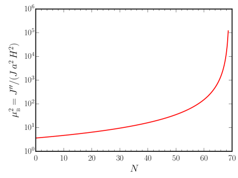
Figure 1: The evolution of the quantity $\mu_{{}_{\mathrm{B}}}^{2}=J^{\prime\prime}/(J\,a^{2}\,H^{2})$, with $J$ being given by the coupling function (31), as it occurs in the case of slow roll inflation driven by the quadratic potential (in this context, see Sec. III), has been plotted as a function of e-folds $N$. We have set $\alpha=-1/\epsilon_{1\ast}\simeq-10^{2}$, where $\epsilon_{1\ast}$ is the value of the first slow roll parameter when the pivot scale $k_{\ast}$ leaves the Hubble radius. For the value of the parameter $m$ (describing the quadratic potential) and the initial conditions we have worked with, we find that the pivot scale $k_{\ast}$ leaves the Hubble radius at the e-fold of $N=18.63$. We find that $\mu_{{}_{\mathrm{B}}}^{2}\simeq 6$ near $N\simeq 18$, which is necessary to result in a scale invariant spectrum for the magnetic field. However, since the first slow roll parameter $\epsilon_{1}$ is not a constant, $\mu_{{}_{\mathrm{B}}}^{2}$ changes with time and, actually, grows to a large value towards the end of inflation. Apart from affecting the shape of the spectra of the electromagnetic fields, we find that, a large value of $\alpha$ also leads to exceedingly large values of the electromagnetic vector potential at either the early or the late stages of inflation.

We have chosen the parameter $\alpha$ so that $\mu_{{}_{\mathrm{B}}}^{2}\simeq 6$ when the pivot scale leaves the Hubble radius, which is required to lead to a nearly scale invariant spectrum for the magnetic field. But, since $\epsilon_{1}$ changes with time, the quantity $\mu_{{}_{\mathrm{B}}}^{2}$ grows to large values at later times. Such a behavior of $\mu_{{}_{\mathrm{B}}}^{2}$ not only affects the shape of the spectra of the electromagnetic fields, it influences their amplitude as well. Importantly, we find that, in general, a large value for $\alpha$ leads to rather large values for the electromagnetic vector potential at either early or late times.

Phenomenologically, the only way out of this difficulty is to choose the index $\alpha$ in $J(R)$ [cf. Eq. (31)] to be dependent on time. In order to arrive at a scale invariant power spectrum for the magnetic field, one may work with a coupling function of the following form:

$$J=\left(\frac{R}{6\,H_{\mathrm{e}}^{2}}\right)^{\alpha(N)}=\left[\frac{H^{2}\,\left(2-\epsilon_{1}\right)}{H_{\mathrm{e}}^{2}}\right]^{\alpha(N)}$$ (33)

and choose $\alpha(N)$ to be

$$\alpha(N)=\frac{2\,\left(N-N_{\mathrm{e}}\right)}{{\mathrm{ln}}\,\left[H^{2}\,\left(2-\epsilon_{1}\right)/H_{\mathrm{e}}^{2}\right]},$$ (34)

where $H_{\mathrm{e}}$ and $N_{\mathrm{e}}$ denote the Hubble parameter and the e-fold at the end of inflation. Such a choice essentially leads to $J(R)\propto a^{2}$, thereby guaranteeing a scale invariant spectrum for the magnetic field. However, the action (29) of the electromagnetic field described by the coupling function (31) with an $\alpha$ that depends on time will not be invariant under general coordinate transformations. A theory which breaks general covariance seems unattractive and is also quite likely to be unviable.

II.4 Strength of magnetic fields at the present epoch

The spectrum of magnetic fields evaluated at the end of inflation allows us to arrive at their strengths at the present epoch. In the conventional picture, the epoch of reheating is supposed to succeed inflation. During reheating, when the energy from the inflaton is being transferred to the particles constituting matter, the universe is expected to be filled with a plasma of charged particles. The creation of charged particles results in a rapid rise in the conductivity of the plasma during reheating and, as a result, the electric fields are shorted out, i.e. they decay exponentially. Thereafter, the magnetic fields are supposed to evolve adiabatically with the expansion of the universe due to the fact that the fluxes freeze in the highly conducting plasma (for a discussion on these points, see, for instance, Refs. [5, 8]).

Let us consider the simple scenario wherein reheating occurs instantaneously at the termination of inflation. In such a case, the spectrum of the magnetic field today, say, $\mathcal{P}_{{}_{\mathrm{B}}}^{0}(k)$, can be related to the spectrum $\mathcal{P}_{{}_{\mathrm{B}}}(k)$ at the end of inflation as follows:

$$\mathcal{P}_{{}_{\mathrm{B}}}^{0}(k)\simeq\mathcal{P}_{{}_{\mathrm{B}}}(k)\,\left(\frac{a_{\mathrm{e}}}{a_{0}}\right)^{4},$$ (35)

where $a_{\mathrm{e}}$ is the scale factor at the end of inflation, while $a_{0}$ denotes the scale factor today. The ratio $a_{\mathrm{e}}/{a_{0}}$ can be determined from the conservation of entropy, i.e. the constancy of the quantity $g_{\mathrm{s}}\,T^{3}\,a^{3}$ from the end of inflation until today, where $T$ is the temperature of radiation at a given epoch and $g_{\mathrm{s}}$ represents the effective relativistic degrees of freedom that contribute to the entropy. As a result, we can write

$$\frac{a_{0}}{a_{\mathrm{e}}}=\left(\frac{g_{\mathrm{s},\mathrm{e}}}{g_{\mathrm{s},0}}\right)^{1/3}\,\frac{T_{\mathrm{e}}}{T_{0}},$$ (36)

where $(T_{\mathrm{e}},g_{\mathrm{s},\mathrm{e}})$ and $(T_{0},g_{\mathrm{s},0})$ denote the temperature and the effective number of relativistic degrees of freedom at the onset of the radiation dominated epoch and today, respectively. The quantity $T_{\mathrm{e}}$ can be determined using the fact that, in the case of instantaneous reheating, the energy density at the end of inflation equals that of radiation at the epoch, leading to $\rho_{{}_{\mathrm{I}}}\simeq 3\,H_{{}_{\mathrm{I}}}^{2}\,M_{{}_{\mathrm{Pl}}}^{2}\simeq g_{\mathrm{r},\mathrm{e}}\,(\pi^{2}/30)\,T_{\mathrm{e}}^{4}$, where $g_{\mathrm{r}}$ denotes the effective number of relativistic degrees that contribute to the energy density of radiation. For simplicity, if we assume that $g_{\mathrm{r}}\simeq g_{\mathrm{s}}$, upon using the above relation, we can arrive at

$$\frac{a_{0}}{a_{\mathrm{e}}}\simeq\left(\frac{g_{\mathrm{e}}}{g_{0}}\right)^{1/3}\,\left(\frac{90\,H_{{}_{\mathrm{I}}}^{2}\,M_{{}_{\mathrm{Pl}}}^{2}}{g_{\mathrm{e}}\,\pi^{2}\,T_{0}^{4}}\right)^{1/4}.$$ (37)

If we consider $g_{\mathrm{e}}=106.75$, since $g_{0}=3.36$ and $T_{0}=2.725\,\mathrm{K}$, we obtain that

$$\frac{a_{0}}{a_{\mathrm{e}}}\simeq 2.8\times 10^{28}\,\left(\frac{H_{{}_{\mathrm{I}}}}{10^{-5}\,M_{{}_{\mathrm{Pl}}}}\right)^{1/2}.$$ (38)

Given the scale invariant spectrum (27a) for the magnetic field at the end of inflation in the $n=2$, helical case, upon substituting the above expression for $a_{0}/a_{\mathrm{e}}$ in Eq. (35), we can estimate the present day strength of the magnetic field, say, $B_{0}$ (at any scale), to be

$$B_{0}\simeq 4.5\times 10^{-12}\,\left(\frac{H_{{}_{\mathrm{I}}}}{10^{-5}\,M_{{}_{\mathrm{Pl}}}}\right)\,f^{1/2}(\gamma)\;\mathrm{G},$$ (39)

where the function $f(\gamma)$ is given by Eq. (28). Recall that, in the non-helical case, since $\gamma=0$, we have $f(\gamma)=1$. Therefore, when parity is conserved, if inflation occurs over energy scales such that $10^{-10}\lesssim H_{{}_{\mathrm{I}}}/M_{{}_{\mathrm{Pl}}}\lesssim 10^{-5}$, then inflationary magnetogenesis can be expected to lead to magnetic fields of strength in the range $10^{-17}\lesssim B_{0}\lesssim 10^{-11}\,\mathrm{G}$ today. As we shall discuss later, to avoid backreaction due to the generated electromagnetic fields, the helicity parameter $\gamma$ is constrained to be less than about $2.5$. We find that, when parity is violated, the above-mentioned strengths of the magnetic fields today are amplified by a factor of about $34$ when $\gamma\simeq 1$ and by a factor of about $4.4\times 10^{3}$ when $\gamma\simeq 2$.

III Coupling function in slow roll inflationary models

Before we go on to discuss inflationary models leading to features in the scalar power spectrum, we shall evaluate the spectra of electromagnetic fields generated in slow roll inflation. Specifically, we shall discuss the forms of the coupling function $J(\phi)$ that are required to generate nearly scale invariant magnetic fields in slow roll inflation. This simple exercise proves to be instructive when we later consider situations involving departures from slow roll.

Note that, in terms of e-folds, the coupling function (6) is given by $J(N)=\mathrm{exp}\,[n\,(N-N_{\mathrm{e}})]$, where $N_{\mathrm{e}}$ denotes the e-fold at the end of inflation. Since the evolution of the field $\phi(N)$ will depend on the inflationary potential, it should be evident that a specific function $J(\phi)$ will not lead to the above-mentioned form of $J(N)$ in all the models. We shall now construct the coupling functions $J(\phi)$ that result in the required $J(N)$ in some of the popular inflationary models that permit slow roll inflation. For these choices of the coupling functions, assuming $n=2$, we shall also numerically evaluate the power spectra of the electromagnetic fields in these potentials. We shall impose the initial conditions on the electromagnetic modes when $k\simeq 10^{2}\,\sqrt{J^{\prime\prime}/J}$, evolve the modes until late times and evaluate the spectra at the end of inflation.

We shall consider three forms for the potential $V(\phi)$. The first model we shall consider is the popular quadratic potential given by

$$V(\phi)=\frac{m^{2}}{2}\,\phi^{2}.$$ (40)

In such a potential, it is well known that, under the slow roll approximation, the evolution of the field can be expressed as

$$\phi^{2}(N)\simeq\phi_{\mathrm{e}}^{2}+4\,\,(N_{\mathrm{e}}-N)\,M_{{}_{\mathrm{Pl}}}^{2},\$$ (41)

where $\phi_{\mathrm{e}}\simeq\sqrt{2}\,M_{{}_{\mathrm{Pl}}}$ denotes the value of the field at the end of inflation. Clearly, we can arrive at the form of $J(N)$ that we desire if we choose $J(\phi)$ to be (in this context, see Refs. [35, 34])

$$J(\phi)=\mathrm{exp}\,\left[-\frac{n}{4\,M_{{}_{\mathrm{Pl}}}^{2}}\,(\phi^{2}-\phi_{\mathrm{e}}^{2})\right].$$ (42)

Recall that, COBE normalization determines the value of the parameter $m$, and we find that we need to choose $m=7.18\times 10^{-6}\,M_{{}_{\mathrm{Pl}}}$ to arrive at the observed scalar amplitude at the pivot scale [50]. To evolve the background, we shall choose the initial values of the field and the first slow roll parameter to be $\phi_{\mathrm{i}}=16.5\,M_{{}_{\mathrm{Pl}}}$ and $\epsilon_{1\mathrm{i}}=7.346\times 10^{-3}$, respectively. In such a case, we find that inflation lasts for $68.6$ e-folds in the model.

The second example we shall consider is the small field model described by the potential

$$V(\phi)=V_{0}\,\left[1-\left(\frac{\phi}{\mu}\right)^{q}\right]$$ (43)

and we shall focus on the case wherein $q=2$. On working in the slow roll approximation, the evolution of the field in such a model can be written as

$$\mu^{2}\,\mathrm{ln}\left(\frac{\phi}{\phi_{\mathrm{e}}}\right)-\frac{1}{2}\,\left(\phi^{2}-\phi_{\mathrm{e}}^{2}\right)\simeq 2\,(N-N_{\mathrm{e}})\,M_{{}_{\mathrm{Pl}}}^{2},$$ (44)

with $\phi_{\mathrm{e}}$ again denoting the value of the field at the end of inflation. Hence, we can arrive at the $J(N)$ of our interest if we choose the coupling function $J(\phi)$ to be

$$J(\phi)\simeq\left(\frac{\phi}{\phi_{\mathrm{e}}}\right)^{n\,\mu^{2}/2M_{{}_{\mathrm{Pl}}}^{2}}\,\mathrm{exp}\,\left[-\frac{n}{4\,M_{{}_{\mathrm{Pl}}}^{2}}\,(\phi^{2}-\phi_{\mathrm{e}}^{2})\right].$$ (45)

If we assume that $\mu\gg M_{{}_{\mathrm{Pl}}}$, then we find that $\phi_{\mathrm{e}}\simeq\mu$. We shall choose $\mu=10\,M_{{}_{\mathrm{Pl}}}$. We find that COBE normalization leads to $V_{0}=5.38\times 10^{-10}\,M_{{}_{\mathrm{Pl}}}^{4}$. We have set the initial values of the field and the first slow roll parameter to be $\phi_{\mathrm{i}}=1.6\,M_{{}_{\mathrm{Pl}}}$ and $\epsilon_{1\mathrm{i}}=5.39\times 10^{-4}$, which lead to about $68.4$ e-folds of inflation.

The third case that we shall consider is the Starobinsky model described by the potential

$$V(\phi)=V_{0}\,\left[1-\mathrm{exp}\left(-\sqrt{\frac{2}{3}}\,\frac{\phi}{M_{{}_{\mathrm{Pl}}}}\right)\right]^{2}.$$ (46)

As we shall consider another model due to Starobinsky later, we shall refer to this potential as the first Starobinsky model. In this model, the evolution of the field in the slow roll approximation is described by the expression

$$N-N_{\mathrm{e}} \simeq -\frac{3}{4}\,\biggl{[}\mathrm{exp}\left({\sqrt{\frac{2}{3}}}\,\frac{\phi}{M_{{}_{\mathrm{Pl}}}}\right)-\mathrm{exp}\left({\sqrt{\frac{2}{3}}}\,\frac{\phi_{\mathrm{e}}}{M_{{}_{\mathrm{Pl}}}}\right)$$ (47)

$$-\,\sqrt{\frac{2}{3}}\,\left(\frac{\phi}{M_{{}_{\mathrm{Pl}}}}-\frac{\phi_{\mathrm{e}}}{M_{{}_{\mathrm{Pl}}}}\right)\biggr{]},$$

where the value of the field at the end of inflation, viz. $\phi_{\mathrm{e}}$, is determined by the relation $\mathrm{exp}\,[\sqrt{(2/3)}\,\phi_{\mathrm{e}}/M_{{}_{\mathrm{Pl}}}]\simeq 1+2/\sqrt{3}$. Therefore, to achieve the desired dependence of the coupling function on the scale factor, we can choose $J(\phi)$ in the model to be

$$J(\phi) = \mathrm{exp}\,\biggl{\{}-\frac{3\,n}{4}\,\biggl{[}\mathrm{exp}\left({\sqrt{\frac{2}{3}}}\,\frac{\phi}{M_{{}_{\mathrm{Pl}}}}\right)-\mathrm{exp}\left({\sqrt{\frac{2}{3}}}\,\frac{\phi_{\mathrm{e}}}{M_{{}_{\mathrm{Pl}}}}\right)$$ (48)

$$-\,\sqrt{\frac{2}{3}}\,\left(\frac{\phi}{M_{{}_{\mathrm{Pl}}}}-\frac{\phi_{\mathrm{e}}}{M_{{}_{\mathrm{Pl}}}}\right)\biggr{]}\biggr{\}}.$$

Again, COBE normalization fixes the overall amplitude of the potential to be $V_{0}=1.43\times 10^{-10}\,M_{{}_{\mathrm{Pl}}}^{4}$. We have chosen the initial values of the field and the first slow roll parameter to be $\phi_{\mathrm{i}}=5.6\,M_{{}_{\mathrm{Pl}}}$ and $\epsilon_{1\mathrm{i}}=1.453\times 10^{-4}$. We find that, for the above-mentioned value of $V_{0}$, these initial conditions lead to about $69.5$ e-folds before inflation ends.

Let us now try to understand the amplitude and shape of the spectra of the electromagnetic fields that arise in these models. Evidently, to arrive at a nearly scale invariant spectrum for the magnetic field, we shall choose to work with $n=2$. Since the inflationary models introduced above will lead to a scale factor of the slow roll form (rather of the de Sitter type), clearly, we can expect the spectrum of the magnetic field in both the non-helical and helical cases to exhibit a small tilt. Moreover, in these situations, the spectrum of the electric field can be expected to be nearly scale invariant (as the spectrum of the magnetic field) in the helical case, while it can be expected to behave nearly as $k^{2}$ in the non-helical case. In Fig. 2, we have plotted the spectra arising in the three slow roll models that we discussed above.

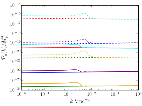
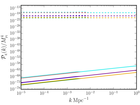
Figure 2: The spectra of the magnetic (on the left) and electric (on the right) fields arising in the three slow roll inflationary models, viz. the quadratic potential (in red), the small field model (in blue) and the first Starobinsky model (in green), have been plotted over the CMB scales. We have also plotted the corresponding spectra when a step has been introduced in these potentials (in cyan, purple and orange, respectively), a scenario we shall discuss later in Subsec. V.1. Moreover, we have plotted the spectra in both the non-helical (as solid lines) and helical (as dashed lines) cases. We have worked with the parameters mentioned in the text and we have set $n=2$ in arriving at the spectra. In the helical case, we have set $\gamma=1$. We should mention that the shapes and amplitudes of these numerically evaluated spectra roughly match the analytical estimates discussed in the text. For instance, the spectrum of the magnetic field is nearly scale invariant in all the models (and in both the non-helical and helical cases), modulo a small step-like feature that arises when a step is introduced in the potential. Also, the spectrum of the electric field behaves as $k^{2}$ in the non-helical case and it is scale invariant and matches the amplitude of the magnetic field in the helical case, as we had discussed. Further, clearly, the amplitude of the spectrum of the helical magnetic field is about $10^{3}$ larger than the amplitude of the non-helical field, as expected when $\gamma=1$.

Interestingly, we find that, while the power spectrum for the non-helical magnetic field arising in the case of the quadratic potential has a small red tilt, the spectral tilt happens to be slightly blue in the cases of the small field and the Starobinsky models. One may have naively imagined that, in such situations, it would be possible to express the spectral tilts $n_{{}_{\mathrm{B}}}$ and $n_{{}_{\mathrm{E}}}$ completely in terms of the slow roll parameters. This would have indeed been true had we assumed that $J\propto a^{n}$ and worked with the slow roll expression for the scale factor (in this context, see App. A). However, our choices for the coupling functions [viz. Eqs. (42), (45) and (48)] do not exactly mimic the behavior of $J\propto a^{n}$, but contain small departures from it. As a result of these deviations, we find that the spectral indices depend on the parameters describing the potential apart from the slow roll parameters. In App. A, we show that, a simple analytical estimate of the spectral indices indeed match the results we have numerically obtained in all these three cases.

Let us now estimate the amplitude of the electromagnetic spectra in the slow roll models. Let us first consider the non-helical case. It can be easily shown that, when $n=2$, the amplitude of the spectra of the magnetic and electric fields at the pivot scale $k_{\ast}$ can be expressed as [cf. Eqs. (14)]

$$\frac{\mathcal{P}_{{}_{\mathrm{B}}}(k)}{M_{{}_{\mathrm{Pl}}}^{4}} \simeq \frac{9\,\pi^{2}}{16}\,\left(r\,A_{\mathrm{s}}\right)^{2},$$ (49a)

$$\frac{\mathcal{P}_{{}_{\mathrm{E}}}(k)}{M_{{}_{\mathrm{Pl}}}^{4}} \simeq \frac{\mathcal{P}_{{}_{\mathrm{B}}}(k)}{9\,M_{{}_{\mathrm{Pl}}}^{4}}\,\left(\frac{k_{\ast}}{k_{\mathrm{e}}}\right)^{2}\simeq\frac{\mathcal{P}_{{}_{\mathrm{B}}}(k)}{9\,M_{{}_{\mathrm{Pl}}}^{4}}\,\mathrm{e}^{-100}.$$ (49b)

In these expressions, $A_{\mathrm{s}}=2.1\times 10^{-9}$ denotes the observed amplitude of the scalar power spectrum at the pivot scale and $r$ represents the tensor-to-scalar ratio [50, 85]. Note that, we have set $k_{\mathrm{e}}\simeq-1/\eta_{\mathrm{e}}$, where, as we have indicated earlier, $k_{\mathrm{e}}$ is the wave number that leaves the Hubble radius at the end of inflation. Also, in arriving at the final equality in the above expression for $\mathcal{P}_{{}_{\mathrm{E}}}(k)$, we have assumed that the pivot scale leaves the Hubble radius $50$ e-folds before the end of inflation, as we have done in the numerical evaluation of the electromagnetic spectra plotted in Fig. 2. In the three slow roll inflationary models of our interest, viz. the quadratic potential, the small field model and the Starobinsky model, the tensor-to-scalar ratio can be easily estimated to be $r\simeq(1.6\times 10^{-1},5.79\times 10^{-2},4.8\times 10^{-3})$. The above expressions then suggest that these models will generate non-helical magnetic fields of amplitudes $\mathcal{P}_{{}_{\mathrm{B}}}(k)\simeq(6.27\times 10^{-19},8.21\times 10^{-20},5.64\times 10^{-22})\,M_{{}_{\mathrm{Pl}}}^{4}$. Moreover, according to expressions above, $\mathcal{P}_{{}_{\mathrm{B}}}(k)\simeq 10^{-20}\,M_{{}_{\mathrm{Pl}}}^{4}$ implies that $\mathcal{P}_{{}_{\mathrm{E}}}(k)\simeq 10^{-66}\,M_{{}_{\mathrm{Pl}}}^{4}$. These estimates roughly match the results we have arrived at numerically and have illustrated in Fig. 2. Further, since $\mathcal{P}_{{}_{\mathrm{B}}}(k)\gg\mathcal{P}_{{}_{\mathrm{E}}}(k)$ in the non-helical case, clearly, most of the energy in the generated electromagnetic fields is in the magnetic field. Lastly, since $\mathcal{P}_{{}_{\mathrm{B}}}(k)/M_{{}_{\mathrm{Pl}}}^{4}\simeq(H_{{}_{\mathrm{I}}}/M_{{}_{\mathrm{Pl}}})^{4}\lesssim 10^{-20}$ in these models, we have $\mathcal{P}_{{}_{\mathrm{B}}}(k)/M_{{}_{\mathrm{Pl}}}^{4}\ll\rho_{{}_{\mathrm{I}}}/M_{{}_{\mathrm{Pl}}}^{4}\sim H_{{}_{\mathrm{I}}}^{2}/M_{{}_{\mathrm{Pl}}}^{2}$, where, recall that, $\rho_{{}_{\mathrm{I}}}$ is the energy density of the inflaton. This suggests that the energy density in the generated electromagnetic field is smaller than the background energy density and hence these scenarios do not suffer from the backreaction problem (for an early discussion in this context, see Ref. [35], for more recent discussions, see Ref. [86, 36]).

Let us now turn to case of the helical electromagnetic fields. In the helical case, when $n=2$, the amplitude of the spectra of the magnetic and electric fields can be expressed as [cf. Eqs. (27)]

$$\frac{\mathcal{P}_{{}_{\mathrm{B}}}(k)}{M_{{}_{\mathrm{Pl}}}^{4}} \simeq \frac{9\,\pi^{2}}{16}\,\left(r\,A_{\mathrm{s}}\right)^{2}\,f(\gamma),$$ (50a)

$$\frac{\mathcal{P}_{{}_{\mathrm{E}}}(k)}{M_{{}_{\mathrm{Pl}}}^{4}} \simeq \frac{\mathcal{P}_{{}_{\mathrm{B}}}(k)}{M_{{}_{\mathrm{Pl}}}^{4}}\,\gamma^{2},$$ (50b)

where $f(\gamma)$ is given by Eq. (28). Note that, in contrast to the non-helical case, the energy density in the electric field is now comparable to that of the magnetic field and, in fact, the contribution due to electric field dominates when $\gamma>1$. Therefore, if we need to avoid backreaction due to the helical electromagnetic fields which have been generated, we require that $\mathcal{P}_{{}_{\mathrm{B}}}(k)+\mathcal{P}_{{}_{\mathrm{E}}}(k)\ll\rho_{{}_{\mathrm{I}}}$. Since we are considering inflationary models wherein $H/M_{{}_{\mathrm{Pl}}}\lesssim 10^{-5}$, on using the above expressions for the spectra of the electromagnetic fields, we find that the condition for avoiding backreaction leads to $f(\gamma)\,(1+\gamma^{2})\lesssim 10^{10}$. This limits the value of $\gamma$ to be $\gamma\lesssim 2.5$. In Fig. 2, assuming $\gamma=1$, we have also plotted the spectra of the helical electromagnetic fields in the three inflationary models discussed above. When $\gamma=1$, we find that $f(\gamma)\simeq 10^{3}$. As should be evident from the figure, the spectra of the helical magnetic fields is indeed amplified by the factor of $10^{3}$ when compared to the non-helical case in all the models. Also, it should be clear that, the spectra of the helical electric and magnetic fields are comparable, as expected.

IV Inflationary models leading to features in the scalar power spectrum

In this section, we shall discuss specific examples wherein deviations from slow roll inflation lead to features in the scalar power spectrum. In due course, we shall discuss the effects of such deviations on the spectra of the electromagnetic fields. When departures from slow roll occur, in general, the background and the modes describing the scalar perturbations prove to be difficult to evaluate analytically, and one resorts to numerics. We shall begin by recalling a few essential points regarding the evaluation of the scalar power spectrum.

Let $f_{k}$ denote the Fourier modes associated with the curvature perturbation. The modes $f_{k}$ satisfy the differential equation (see, for instance, the reviews [87, 88, 89, 90, 91, 92, 93, 94, 95, 96, 97])

$$f_{k}^{\prime\prime}+2\,\frac{z^{\prime}}{z}\,f_{k}^{\prime}+k^{2}\,f_{k}=0,$$ (51)

where the quantity $z$ is given by $z=\sqrt{2\,\epsilon_{1}}\,M_{{}_{\mathrm{Pl}}}\,a$, with $\epsilon_{1}=-\dot{H}/H^{2}$ being the first slow roll parameter. In terms of the Mukhanov-Sasaki variable $v_{k}=f_{k}\,z$, the above equation reduces to

$$v_{k}^{\prime\prime}+\left(k^{2}-\frac{z^{\prime\prime}}{z}\right)\,v_{k}=0.$$ (52)

The standard Bunch-Davies initial conditions are imposed on the variable $v_{k}$ at very early times when $k\gg\sqrt{z^{\prime\prime}/z}$, which corresponds to the modes being in sub-Hubble regime. The scalar power spectrum is defined as

$$\mathcal{P}_{{}_{\mathrm{S}}}(k)=\frac{k^{3}}{2\,\pi^{2}}\,|f_{k}|^{2}=\frac{k^{3}}{2\,\pi^{2}}\,{\frac{|v_{k}|^{2}}{z^{2}}}.$$ (53)

The modes $f_{k}$ are evolved from the Bunch-Davies initial conditions and the power spectra are evaluated in the super-Hubble regime at late times, i.e. when $k\ll\sqrt{z^{\prime\prime}/z}$. Since the modes oscillate in the sub-Hubble domain and the amplitude of the scalar modes are known to freeze on super-Hubble scales, numerically, one often finds that it is sufficient to evolve the modes from $k\simeq 10^{2}\,\sqrt{z^{\prime\prime}/z}$ and evaluate the power spectrum when $k\simeq 10^{-5}\,\sqrt{z/^{\prime\prime}z}$ (in this context, see, for instance, Ref. [98]).

IV.1 Potentials with a step

The first scenario leading to features in the scalar power spectrum that we shall consider are inflationary potentials wherein a step has been introduced by hand. Given an inflationary model described by the potential $V(\phi)$, we shall introduce a step in the potential as follows (for an early discussion, see Ref. [99]):

$$V_{\mathrm{step}}(\phi)=V(\phi)\,\left[1+\alpha\,\mathrm{tanh}\,\left(\frac{\phi-\phi_{0}}{\Delta\phi}\right)\right],$$ (54)

where, evidently, $\phi_{0}$, $\alpha$ and $\Delta\phi$ denote the location, the height and the width of the step. For the original potential $V(\phi)$, we shall consider the three models admitting slow roll we had discussed in the previous section. Also, as far as the parameters regarding the original potential is concerned, we shall work with the values we had mentioned earlier. Moreover, we shall work with the following values of the three parameters describing the step: $(\phi_{0},\alpha,\Delta\phi)=(14.6616\,M_{{}_{\mathrm{Pl}}},1.55177\times 10^{-3},2.60584\times 10^{-2}\,M_{{}_{\mathrm{Pl}}}),(2.14\,M_{{}_{\mathrm{Pl}}},-0.1153\times 10^{-3},0.0070\,M_{{}_{\mathrm{Pl}}})$ and $(5.3052\,M_{{}_{\mathrm{Pl}}},5.0\times 10^{-5},5.0\times 10^{-3}\,M_{{}_{\mathrm{Pl}}})$ in the cases of the quadratic potential, the small field model and the first Starobinsky model, respectively.

As we described above, to arrive at the scalar power spectrum, we impose the initial conditions on the modes when $k\simeq 10^{2}\,\sqrt{z^{\prime\prime}/z}$ and evaluate the power spectrum when $k\simeq 10^{-5}\,\sqrt{z^{\prime\prime}/z}$. Moreover, in these three models, we shall assume that the pivot scale of $k_{\ast}=0.05\,\mathrm{Mpc}^{-1}$ leaves the Hubble radius $50$ e-folds before the end of inflation. The scalar power spectrum that arises with the introduction of the step in the quadratic potential is illustrated in Fig. 3.

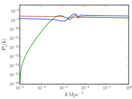
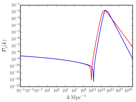
Figure 3: The scalar power spectra with features over the CMB and smaller scales have been plotted in some of the inflationary models that we have considered. We have plotted the scalar spectra with features over the CMB scales (on the left) in the cases of the quadratic potential with a step (in red), the second Starobinsky model described by the linear potential with a sharp change in its slope (in blue), and the first punctuated inflation model (in green). We have also plotted the scalar power spectra with a peak in power at small scales (on the right) that are generated in the ultra slow roll (in red) and the second punctuated (in blue) inflation models. As we shall point out later, the scalar spectra with a sharp rise in power on small scales are often considered to produce significant amount of primordial black holes.

.

As one would expect, the introduction of the step in the potential leads to a short period of deviation from slow roll as the field crosses the step. The deviation from slow roll, in turn, generates a short burst of oscillations in the scalar power spectrum over wave numbers that leave the Hubble radius during the period of departure from slow roll. It is known that such features in the power spectrum can improve the fit to the CMB data to a certain extent [56, 57].

IV.2 Suppressing power on large scales

Since the advent the WMAP data, it has been known that a suppression in power on large scales comparable to the Hubble radius today leads to an improvement in the fit to the CMB data (for earlier discussions, see Refs. [51, 52, 53, 54, 55, 58, 59]; for a recent discussion, see Ref. [62]). In this subsection, we shall discuss two models that have often been considered in this context.

The first example that we shall consider is a model due to Starobinsky, which is governed by the potential [100]

$$V(\phi)=\begin{cases}V_{0}+A_{+}\,(\phi-\phi_{0}),&\text{for $\phi>\phi_{0}$},\\ V_{0}+A_{-}\,(\phi-\phi_{0}),&\text{for $\phi<\phi_{0}$}.\end{cases}$$ (55)

To distinguish from the Starobinsky model (46) which permits slow roll inflation that we had discussed earlier, we shall refer to the above potential as the second Starobinsky model. Evidently, the model consists of a linear potential with a sudden change in its slope at the point $\phi_{0}$. If we assume that the constant term $V_{0}$ in the potential is dominant, then the first slow roll parameter remains small and the scale factor can be described by the de Sitter form. Under this condition, it is possible to arrive at analytical solutions for the evolution of the background [100, 101]. We shall discuss the evolution of the field later, when we consider the coupling between the inflaton and the electromagnetic field. It is found that, as the field crosses $\phi_{0}$, while the first slow roll parameter remains small, the second and the third slow roll parameters turn large leading to a departure from slow roll. Also, notice that the second derivative of the potential is described by a Dirac delta function with its peak at $\phi_{0}$. It is the Dirac delta function that dominates the behavior of the quantity $z^{\prime\prime}/z$ that appears in the Mukhanov-Sasaki equation (52). Working in the de Sitter approximation to describe the scale factor as well as the scalar modes $f_{k}$, the deviation from slow roll could be accounted for by essentially considering the effects due to the Dirac delta function. In fact, under these conditions, it is possible to arrive at an analytical form for the power spectrum [100, 101, 62]. We shall instead arrive at the scalar power spectrum numerically. In order to permit numerical analysis, we shall modify the potential so that the change in the slope is smooth and not abrupt. We shall assume that the potential is given by

$$V(\phi) = V_{0}+\frac{1}{2}\,(A_{+}+A_{-})\,(\phi-\phi_{0})$$ (56)

$$+\,\frac{1}{2}\,(A_{+}-A_{-})\,(\phi-\phi_{0})\,\mathrm{tanh}\left(\frac{\phi-\phi_{0}}{\Delta\phi}\right),\qquad$$

and work with the following values of the parameters involved: $V_{0}=2.98\times 10^{-9}\,M_{{}_{\mathrm{Pl}}}^{4}$, $A_{+}=4.35881\times 10^{-10}\,M_{{}_{\mathrm{Pl}}}^{3}$, $A_{-}=2.499\times 10^{-10}\,M_{{}_{\mathrm{Pl}}}^{3}$, $\phi_{0}=5.628\,M_{{}_{\mathrm{Pl}}}$ and $\Delta\phi=10^{-4}\,\phi_{0}$. We shall choose the initial value of the field and the first slow roll parameter to be $\phi_{\mathrm{i}}=8.4348\,M_{{}_{\mathrm{Pl}}}$ and $\epsilon_{1\mathrm{i}}=10^{-4}$.

The second model that we shall consider is the so-called punctuated inflationary model described by the potential (in this context, see Refs. [54, 55, 62])

$$V(\phi)=\frac{m^{2}}{2}\,\phi^{2}-\frac{2\,m^{2}}{3\,\phi_{0}}\,\phi^{3}+\frac{m^{2}}{4\,\phi_{0}^{2}}\,\phi^{4}.$$ (57)

It is easy to see that this potential contains a point of inflection at $\phi_{0}$. The point of inflection leads to two epochs of slow roll sandwiching a brief period of departure from inflation, which has led to the name of punctuated inflation. As we shall consider another model of punctuated inflation which leads to enhanced power at small scales in the following subsection, we shall refer to the above potential as the first model of punctuated inflation. In this case, we shall work with the following values of the parameters involved: $m=7.17\times 10^{-8}\,M_{{}_{\mathrm{Pl}}}$ and $\phi_{0}=1.9654\,M_{{}_{\mathrm{Pl}}}$. We shall choose the initial values of the field and the first slow roll parameter to be $\phi_{\mathrm{i}}=12.0\,M_{{}_{\mathrm{Pl}}}$ and $\epsilon_{1\mathrm{i}}=2\times 10^{-3}$.

The drawback of these two models is that they lead to much longer epochs of inflation than the nominally required $60$ odd e-folds [62]. In the Starobinsky model (55), we stop the evolution by hand after $72$ e-folds, and assume that the pivot scale leaves the Hubble radius about $44.5$ e-folds earlier. In the case of the punctuated inflationary model (57), inflation ends naturally after nearly $110.5$ e-folds and the pivot scale is assumed to exit the Hubble radius about $91$ e-folds before the termination of inflation. The departure from slow roll in these two potentials leads to a step-like feature in the scalar power spectrum, as illustrated in Fig. 3.

IV.3 Enhancing power on small scales

Over the last few years, there has been a considerable interest in examining models of inflation that lead to enhanced power on scales much smaller than the CMB scales (in this context, see, for example, Refs. [69, 70, 71, 72, 73, 75, 76]). Apart from leading to copious production of primordial black holes, these models can also generate secondary gravitational waves of considerable strengths, which can possibly be detected by the current and forthcoming gravitational wave observatories. Most of these inflationary models contain a point of inflection (just as the model of punctuated inflation we discussed in the previous subsection), which permits a brief period wherein the first slow roll parameter decreases exponentially. Such a period of ultra slow roll proves to be responsible for enhancing the power on small scales in these models.

We shall consider two potentials that lead to enhanced power on small scales. The first model that we shall consider, which leads to a brief period of ultra slow roll, is described by the potential [72]

$$V(\phi) = V_{0}\,\biggl{\{}\mathrm{tanh}\left(\frac{\phi}{\sqrt{6}\,M_{{}_{\mathrm{Pl}}}}\right)$$ (58)

$$+\,A\,\sin\left[\frac{1}{f_{\phi}}\,\mathrm{tanh}\left(\frac{\phi}{\sqrt{6}\,M_{{}_{\mathrm{Pl}}}}\right)\right]\biggr{\}}^{2}.$$

We shall choose to work with the following values of the parameters involved: $V_{0}=2\times 10^{-10}\,M_{{}_{\mathrm{Pl}}}^{4}$, $A=0.130383$ and $f_{\phi}=0.129576$. For these values of the parameters, the point of inflection in the potential is located at $\phi_{0}=1.05\,M_{{}_{\mathrm{Pl}}}$ [75]. Also, if we choose the initial value of the field to be $\phi_{\mathrm{i}}=6.1\,M_{{}_{\mathrm{Pl}}}$, with $\epsilon_{1\mathrm{i}}=10^{-4}$, we obtain about $66$ e-folds of inflation in the model. Moreover, we shall assume that the pivot scale exits the Hubble radius about $56.2$ e-folds prior to the termination of inflation.

The second model that we shall consider which permits punctuated inflation is described by the potential [72, 76]

$$V(\phi) = V_{0}\,\biggl{[}c_{0}+c_{1}\,\tanh\,\left(\frac{\phi}{\sqrt{6}\,M_{{}_{\mathrm{Pl}}}}\right)$$

$$+\,c_{2}\,\tanh^{2}\left(\frac{\phi}{\sqrt{6}\,M_{{}_{\mathrm{Pl}}}}\right)+c_{3}\,\tanh^{3}{\left(\frac{\phi}{\sqrt{6}\,M_{{}_{\mathrm{Pl}}}}\right)}\biggr{]}^{2}.$$

In this case, we shall work with the following values for the parameters involved: $V_{0}=2.1\times 10^{-10}\,M_{{}_{\mathrm{Pl}}}^{4}$, $c_{0}=0.16401$, $c_{1}=0.3$, $c_{2}=-1.426$ and $c_{3}=2.20313$. As in the previous model, this potential also contains a point of inflection. For the above values for the parameters, the point of inflection is located at $\phi_{0}=0.53\,M_{{}_{\mathrm{Pl}}}$. If we set the initial value of the field to be $\phi_{\mathrm{i}}=7.4\,M_{{}_{\mathrm{Pl}}}$ and choose $\epsilon_{1\mathrm{i}}=10^{-3}$, for the above choice of parameters, we find that inflation is terminated after about $67.8$ e-folds. Also, we shall assume that the pivot scale leaves the Hubble radius about $54.5$ e-folds before the end of inflation.

The scalar power spectra that arise in the above two potentials are illustrated in Fig. 3. Note that the power spectra exhibit a sharp rise in power on small scales in these models. As has been repeatedly emphasized in the literature, it is the period of ultra slow roll, with its rather small value for the first slow roll parameter $\epsilon_{1}$, that turns out to be responsible for the increased power in the scalar power spectrum on small scales (in this context, see, for instance, Ref. [102]).

V Effects of deviations from slow roll on the electromagnetic power spectra

Let us now turn to understand the effects of deviations from slow roll on the power spectra of electric and magnetic fields.

V.1 In potentials with a step

As we discussed earlier and illustrated in Fig. 3, the introduction of the step in a potential which otherwise admits only slow roll inflation leads to a short burst of oscillations in the scalar power spectrum. In Sec. III, we had constructed coupling functions $J(\phi)$ [as given by Eqs. (42), (45) and (48)] in the three slow roll models (40), (43) and (46) so that they lead to nearly scale invariant spectra for the magnetic field when $n=2$. Even after the introduction of the step, we have chosen to work with the above mentioned coupling functions $J(\phi)$ that we had constructed in the slow roll approximation. In Fig. 2, we have plotted the resulting spectra of the magnetic and electric fields arrived at numerically in both the non-helical and helical cases. As should be clear from the figure, the step in the inflationary potential only has a small effect on the spectra of the electromagnetic fields. It essentially generates a small step-like feature in the power spectra. This is not surprising since, for the choices of the parameters we have worked with, the step in the potential leads to only a small and brief departure from slow roll inflation.

V.2 In models leading to suppression of power on large scales

In this context, we shall first consider the second Starobinsky model described by the potential (55). As we had mentioned earlier, in the model, the field rolls slowly until it reaches $\phi_{0}$ where the slope of the potential changes from $A_{+}$ to $A-$. In the slow roll approximation, the evolution of the field prior to it crossing $\phi_{0}$ can be determined to be [100, 101]

$$\phi_{+}(N) \simeq -\left(\frac{V_{0}}{A_{+}}-\phi_{0}\right)$$ (60)

$$+\,\biggl{[}\left(\phi_{\mathrm{i}}-\phi_{0}+\frac{V_{0}}{A_{+}}\right)^{2}-2\,M_{{}_{\mathrm{Pl}}}^{2}\,N\biggr{]}^{1/2},\qquad$$

where $\phi_{\mathrm{i}}$ is the initial value of the field (i.e. at $N=0$). If we choose to work with a suitably large value of $V_{0}$ so that it dominates the potential, then the above expression simplifies to be

$$\phi_{+}(N)\simeq\phi_{\mathrm{i}}-\frac{A_{+}\,M_{{}_{\mathrm{Pl}}}^{2}}{V_{0}}\,N.$$ (61)

Evidently, once the field has crossed $\phi_{0}$ and slow roll has been restored, the evolution of the field can be expressed as

$$\phi_{-}(N) \simeq -\left(\frac{V_{0}}{A_{-}}-\phi_{0}\right)$$ (62)

$$+\,\biggl{[}\left(\frac{V_{0}}{A_{-}}\right)^{2}-2\,M_{{}_{\mathrm{Pl}}}^{2}\,(N-N_{0})\biggr{]}^{1/2},$$

where $N_{0}$ denotes the e-fold when the field crosses $\phi_{0}$. If we again assume that $V_{0}$ is dominant, then the above expression reduces to

$$\phi_{-}(N)\simeq\phi_{0}-\frac{A_{-}\,M_{{}_{\mathrm{Pl}}}^{2}}{V_{0}}\,(N-N_{0}).$$ (63)

We should clarify here that, in arriving at the above expressions for the evolution of the field after it has crossed $\phi_{0}$, we have ignored the effects that arise due to the change in the slope. As we had described, the change in the slope causes a brief period of departure from slow roll. If we take into account the effects due to the deviation from slow roll, the evolution of the field after it has crossed $\phi_{0}$ can be obtained to be [100, 101]

$$\phi_{-}(N) \simeq \phi_{0}+\frac{\Delta A\,M_{{}_{\mathrm{Pl}}}^{2}}{3\,V_{0}}\,\left[1-\mathrm{e}^{-3\,(N-N_{0})}\right]$$ (64)

$$-\,\frac{A_{-}\,M_{{}_{\mathrm{Pl}}}^{2}}{V_{0}}\,(N-N_{0}),$$

where $\Delta A=(A_{-}-A_{+})$. Upon comparing the above two equations, it should be obvious that it is the intermediate term that accounts for the departure from slow roll which occurs as the field crosses $\phi_{0}$. On using the above expressions describing the behavior of the field, one can show that, while the first slow roll parameter remains small, the second and the third slow roll parameters turn large as the field crosses $\phi_{0}$.

Let us now turn to constructing the coupling function $J(\phi)$ for the second Starobinsky model. As we had done in the case of the models discussed in Sec. III, we can choose to work with the solutions for the field in the slow roll approximation. If we choose to do so, we are left with two choices, viz. the slow roll solutions (60) and (62) for the field before and after the transition. In other words, we can work with either of the following choices for the coupling function:

$$J_{+}(\phi) = J_{0+}\,\mathrm{exp}\,\biggl{\{}-\frac{n}{2\,M_{{}_{\mathrm{Pl}}}^{2}}\,\biggl{[}\left(\phi_{+}-\phi_{0}+\frac{V_{0}}{A_{+}}\right)^{2}$$ (65a)

$$-\,\left(\phi_{\mathrm{i}}-\phi_{0}+\frac{V_{0}}{A_{+}}\right)^{2}\biggr{]}\biggr{\}},$$

$$J_{-}(\phi) = J_{0-}\,\mathrm{exp}\,\biggl{\{}-\frac{n}{2\,M_{{}_{\mathrm{Pl}}}^{2}}\,\biggl{[}\left(\phi_{-}-\phi_{0}+\frac{V_{0}}{A_{-}}\right)^{2}$$ (65b)

$$-\left(\frac{V_{0}}{A_{-}}\right)^{2}-2\,N_{0}\,M_{{}_{\mathrm{Pl}}}^{2}\biggr{]}\biggr{\}},$$

where the constants $J_{0\pm}$ are to be chosen suitably so that $J_{\pm}(\phi_{\mathrm{e}})=1$, i.e. the value of $J$ is unity at the end of inflation.

The power spectra of the magnetic field for the two coupling functions $J_{\pm}(\phi)$ for the case of $n=2$ are plotted in Fig. 4 for both the non-helical and helical cases.

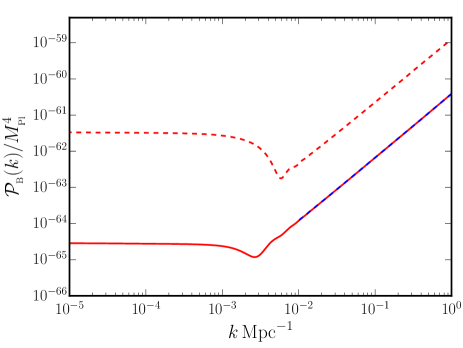
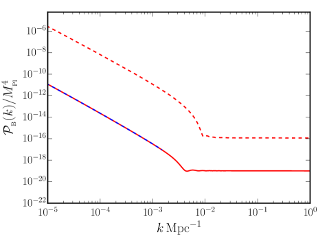
Figure 4: The power spectra of the magnetic field arising in the second Starobinsky model for the two choices of coupling functions $J_{+}(\phi)$ (on the left) and $J_{-}(\phi)$ (on the right) [cf. Eqs. (65)] have been plotted for $n=2$ in the non-helical (in solid red) as well as the helical (in dashed red) cases. A linear fit (indicated in dashed blue) to the non-helical power spectra over the small and the large scales (on the left and the right) lead to the spectral indices $n_{{}_{\mathrm{B}}}=1.75$ and $n_{{}_{\mathrm{B}}}=-2.72$, respectively. For the values of the parameters we have worked with, the analytical estimates for these indices prove to be $n_{{}_{\mathrm{B}}}=1.71$ and $n_{{}_{\mathrm{B}}}=-2.98$, which are close to the numerically determined values. As in Fig. 2, we have set the helicity parameter $\gamma$ to be unity. Moreover, note that, for $\gamma=1$, the spectra of the magnetic field over the scale invariant domain is about $10^{3}$ times larger in the helical case when compared to the non-helical one, as we had estimated earlier. Lastly, we should add that, when the coupling function is given by $J_{-}(\phi)$, the strength of the magnetic fields generated is fairly large and hence the scenario will lead to a significant backreaction.

A few points needs to be emphasized regarding the spectra we have obtained. Firstly, the spectra are scale invariant only over either large or small scales. Let $k_{0}$ be the mode which leaves the Hubble radius when the field crosses $\phi_{0}$. Then, clearly, for the choice of the coupling functions $J_{+}(\phi)$ and $J_{-}(\phi)$, the magnetic field spectra are scale invariant only over $k<k_{0}$ and $k>k_{0}$, respectively. This should not come as a surprise as the coupling functions $J_{\pm}(\phi)$ have been constructed based on the behavior of the field in the slow roll approximation before and after it crosses $\phi_{0}$. Secondly, when $n=2$, for the coupling function $J_{+}(\phi)$, the spectral index of the magnetic field for $k>k_{0}$ can be estimated to be $n_{{}_{\mathrm{B}}}=-4\,\Delta A/A_{+}$, while for the function $J_{-}(\phi)$ the index over large scales can be determined to be $n_{{}_{\mathrm{B}}}=4\,\Delta A/A_{-}$. Since $\Delta A=(A_{-}-A_{+})<0$, $n_{{}_{\mathrm{B}}}>0$ (i.e. the spectrum is blue) in the first case and $n_{{}_{\mathrm{B}}}<0$ (i.e. the spectrum is red) in the second. These estimates are indeed corroborated by the numerical results we have plotted in Fig. 4. Thirdly, while the amplitude of the magnetic field is considerably suppressed over large scales if we work with the coupling function $J_{+}(\phi)$, it is considerably enhanced over these scales in the case of $J_{-}(\phi)$. In fact, for the choice $J_{-}(\phi)$, the strength of the electromagnetic fields on large scales are considerable and hence they will lead to a significant backreaction.

Let us now turn to the first punctuated inflation model described by the potential (57). It proves to be difficult to obtain an analytical solution for the evolution of the background scalar field in such a potential. Therefore, we shall solve for the background numerically to first arrive at $\phi(N)$. We then choose a quadratic function of the form $N(\phi)=a_{1}\,(\phi^{2}/M_{{}_{\mathrm{Pl}}}^{2})+b_{1}\,(\phi/M_{{}_{\mathrm{Pl}}})+c_{1}$ to fit the numerical solution we have obtained in the initial slow roll regime. When doing so, for the specific values of the parameters of the potential and the initial conditions that we have worked with, we obtain the values of the three dimensionless fitting parameters to be $(a_{1},b_{1},c_{1})=(-0.104,-0.0408,15.949)$. Finally, to evaluate the spectra of the electromagnetic fields, we shall work with a coupling function of the form

$$J(\phi)=\mathrm{exp}\,\left\{n\,\left[a_{1}\,\left(\frac{\phi^{2}-\phi_{\mathrm{e}}^{2}}{M_{{}_{\mathrm{Pl}}}^{2}}\right)+b_{1}\,\left(\frac{\phi-\phi_{\mathrm{e}}}{M_{{}_{\mathrm{Pl}}}}\right)\right]\right\}$$ (66)

and, note that, $J(\phi)$ reduces to unity at $\phi_{\mathrm{e}}$, as required. In Fig. 5, we have plotted the spectra of the resulting magnetic and electric fields in both the non-helical and helical cases for $n=2$.

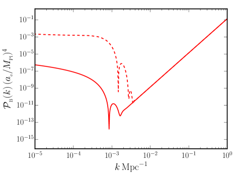
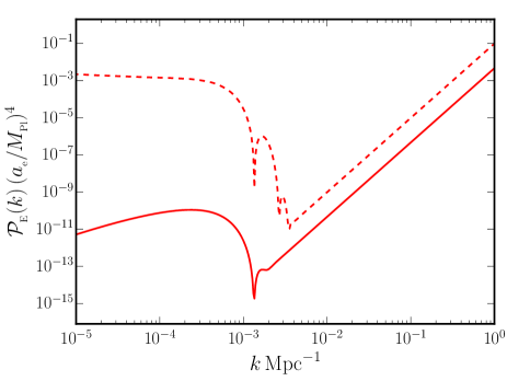
Figure 5: The spectra of the magnetic (on the left) and electric (on the right) fields arising in the case of the first punctuated inflation model (57) have been plotted for both the non-helical (in solid red) and helical (in dashed red) cases. In arriving at these spectra, we have worked with the coupling function (66) and, as earlier, we have set the helicity parameter $\gamma$ to be unity. As expected, over the large scales, when the modes leave the Hubble radius during the initial stages of slow roll inflation, the spectra of the magnetic as well as the electric fields in the helical case are nearly scale invariant and also have roughly the same amplitude. Moreover, the amplitude of the helical magnetic fields are $10^{3}$ times greater in amplitude than the non-helical fields over the scale invariant domain, as one may have guessed. Further, note that the spectra behave as $k^{4}$ over small scales. This behavior can be attributed to the fact that, as the background scalar field approaches the point the inflection, leading to an epoch of ultra slow roll inflation, the non-minimal coupling function $J$ hardly evolves. We should point out that, in the above plots, we have multiplied the spectra of the electromagnetic fields by the factor of by $a_{\mathrm{e}}^{4}$ (in contrast to the other figures) since their amplitudes turn out to be extremely small otherwise. As will be evident from the discussion in the following subsection, the rather small amplitudes in these cases can be attributed to a very early onset of the ultra slow roll epoch required to suppress the scalar power on the largest scales.

We need to highlight a few points regarding the figure. The spectra of the electric and magnetic fields in the helical case and the spectrum of the magnetic field in the non-helical case are scale invariant over large scale modes that leave the Hubble radius during the initial stages of slow roll. Also, over the scale invariant domain, the helical amplitudes are $10^{3}$ times larger than the non-helical amplitudes, as expected for $\gamma=1$. For the choice of the coupling function that we have worked with, we find that, the spectra of both the magnetic and electric fields behave as $k^{4}$ (in the absence as well as in the presence of helicity) over the small scale modes which leave the Hubble radius at later stages. As we shall discuss in more detail in the following section, when the field approaches the point of inflection in the potential and enters a phase of ultra slow roll inflation, the coupling function $J$ hardly changes. This implies that $J^{\prime\prime}/J\simeq 0$, which is responsible for the $k^{4}$ behavior of the spectra at small scales. We should also point out that this behavior significantly suppresses the scale invariant amplitude of the magnetic field over large scales.

The two examples discussed in this subsection point to the fact that unless the coupling function is suitably chosen, strong departures from slow roll inflation result in spectra of magnetic fields that contain significant deviations from scale invariance.

V.3 In models leading to enhanced power on small scales

Let us now turn to the two models described by the potentials (58) and (LABEL:eq:pi2) that lead to enhanced scalar power on small scales. As in the case of the first punctuated inflation model we discussed in the previous subsection, these models too lead to an epoch of ultra slow roll inflation wherein the first slow roll parameter decreases exponentially over a short period before it starts rising leading to an end of inflation. It is the sharp decrease in the first slow roll parameter that is responsible for the rise in the scalar power in such models (in this context, see Refs. [69, 70, 71, 72, 73, 75, 76]).

In these models, one chooses the parameters of the background potential as well as the initial conditions such that there occurs an extended period of slow roll inflation which generates scalar and tensor power spectra that are consistent with the CMB observations on large scales. If we require a nearly scale invariant spectrum of the magnetic field over the CMB scales, then, evidently, we need to choose a coupling function $J(\phi)$ that is based on the evolution of the field during the long initial epoch of slow roll inflation. Since the potentials (58) and (LABEL:eq:pi2) do not seem to admit simple analytical solutions, we repeat the exercise we had carried out in the case of the first punctuated inflation model. Utilizing the numerical solution, we arrive at $N(\phi)$ and fit a polynomial to describe the function. We find that we can fit fourth and sixth order polynomials to describe the $N(\phi)$ in the potentials (58) and (LABEL:eq:pi2). The coupling functions that we shall work with in these two cases can be expressed as

$$J(\phi) = \mathrm{exp}\,\Biggl{\{}n\,\biggl{[}a_{2}\,\left(\frac{\phi^{4}-\phi_{\mathrm{e}}^{4}}{M_{{}_{\mathrm{Pl}}}^{4}}\right)+b_{2}\,\left(\frac{\phi^{3}-\phi_{\mathrm{e}}^{3}}{M_{{}_{\mathrm{Pl}}}^{3}}\right)$$ (67a)

$$+\,c_{2}\,\left(\frac{\phi^{2}-\phi_{\mathrm{e}}^{2}}{M_{{}_{\mathrm{Pl}}}^{2}}\right)+d_{2}\,\left(\frac{\phi-\phi_{\mathrm{e}}}{M_{{}_{\mathrm{Pl}}}}\right)\biggr{]}\Biggr{\}},$$

$$J(\phi) = \mathrm{exp}\,\Biggl{\{}n\,\biggl{[}a_{3}\,\left(\frac{\phi^{6}-\phi_{\mathrm{e}}^{6}}{M_{{}_{\mathrm{Pl}}}^{6}}\right)+b_{3}\,\left(\frac{\phi^{5}-\phi_{\mathrm{e}}^{5}}{M_{{}_{\mathrm{Pl}}}^{5}}\right)$$ (67b)

$$+\,c_{3}\,\left(\frac{\phi^{4}-\phi_{\mathrm{e}}^{4}}{M_{{}_{\mathrm{Pl}}}^{4}}\right)+d_{3}\,\left(\frac{\phi^{3}-\phi_{\mathrm{e}}^{3}}{M_{{}_{\mathrm{Pl}}}^{3}}\right)$$

$$+\,e_{3}\,\left(\frac{\phi^{2}-\phi_{\mathrm{e}}^{2}}{M_{{}_{\mathrm{Pl}}}^{2}}\right)+f_{3}\,\left(\frac{\phi-\phi_{\mathrm{e}}}{M_{{}_{\mathrm{Pl}}}}\right)\biggr{]}\Biggr{\}},\qquad\qquad$$

with the dimensionless fitting parameters being given by $(a_{2},b_{2},c_{2},d_{2})$ $=(-0.184,1.822,-7.040,10.676)$ and $(a_{3},b_{3},c_{3},d_{3},e_{3},f_{3})$ $=(-1.53\times 10^{-3},2.37\times 10^{-2},-0.158,0.439,-0.459,-0.778)$, respectively.

In Fig. 6, we have plotted the spectra of the electromagnetic fields that arise for the above choices of the coupling functions in the two models of our interest.

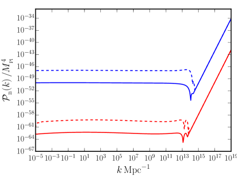
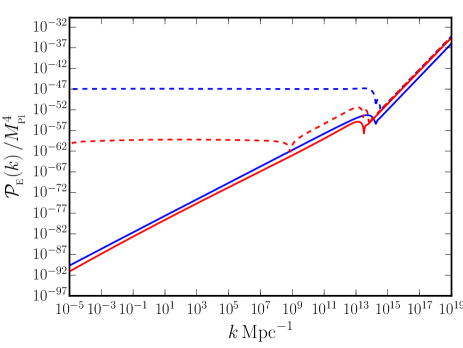
Figure 6: The spectra of the magnetic (on the left) and electric (on the right) fields arising in the ultra slow roll inflationary model (58) (in red) and the second punctuated inflationary model (LABEL:eq:pi2) (in blue) have been plotted in the non-helical (as solid lines) and helical (as dashed lines) cases, respectively. Note that we have worked with the coupling functions (67) to arrive at these spectra. Also, we have chosen $n=2$ and set $\gamma=1$, as we have done earlier. Clearly, the spectra of the electromagnetic fields in both the helical and non-helical cases are along expected lines, as we have discussed in the text. In particular, we should point out that the spectra in the two models behave as $k^{4}$ at large wave numbers. This behavior arises due to the fact the the coupling functions cease to evolve as the field approaches the point of inflection in these models. In such a situation, the electromagnetic modes effectively behave as in the conformally invariant case, leading to the $k^{4}$ behavior. We should also add that, apart from changing the shape of the spectra at small scales, the background evolution significantly suppresses the power in the spectra on large scales.

We should mention that, in arriving at the spectra, we have set $n=2$ and $\gamma=1$, as we have done before. The following points are clear from the figure. Note that the spectra of the magnetic fields in both the non-helical and helical cases are nearly scale invariant over large scales. This is because the coupling functions have been determined by the slow roll behavior of the field. Also, as we have seen earlier, the magnitude of the helical magnetic field is about $10^{3}$ larger than the non-helical field over the scale invariant domain. Moreover, over large scales, as expected, the spectrum of the electric field behaves as $k^{2}$ in the non-helical case and is nearly scale invariant with an amplitude comparable to the spectrum of the magnetic field in the helical case. Further, at small scales, all the spectra behave as $k^{4}$ for the same reasons as we had encountered in the case of the first punctuated inflation model (57). When the background scalar field approaches the point of inflection in these models, the coupling functions $J$ hardly evolve (in this context, see Fig. 7) and the electromagnetic modes effectively behave as in the conformally invariant case leading to the $k^{4}$ behavior. Lastly, we should mention that such a background behavior not only changes the shape of the spectra of the electromagnetic fields at small scales, it also suppresses the scale invariant amplitudes of the spectra at large scales.

V.4 An analytical estimate

In this subsection, we shall analytically arrive at the power spectra of the electromagnetic fields in models which permit ultra slow roll inflation and lead to enhanced scalar power on small scales.

V.4.1 A simple approximation

Recall that, in these scenarios, we had constructed the coupling function $J(\phi)$ so that we obtain a scale invariant spectrum for the magnetic field on large scales [cf. Eqs. (67); also see Eq. (66)]. In order to achieve such a scale invariant spectrum, during the initial stage of slow roll inflation, let us assume that $J(\eta)\propto a^{2}$. Note that, in these models, for our choices of the dependence of the coupling function on the field, we find that $J$ freezes when the epoch of ultra slow roll sets in. This is evident from Fig. 7 wherein we have plotted the evolution of the coupling function in the first and second models of punctuated inflation [cf. Eqs. (57) and (LABEL:eq:pi2)] as well as in the model of ultra slow roll inflation [cf. Eq. (58)]. Therefore, we can assume that, after a time, say, $\eta_{1}$, $J(\eta)\simeq\mathrm{constant}$. In such a case, during the initial stage, the electromagnetic modes ${\mathcal{A}}_{k}$ can be easily obtained to be

$${\mathcal{A}}_{k}^{\mathrm{I}}(\eta)=\frac{1}{\sqrt{2\,k}}\,\left(1-\frac{3\,i}{k\,\eta}-\frac{3}{k^{2}\,\eta^{2}}\right)\,\mathrm{e}^{-i\,k\,\eta}.$$ (68)

It should be evident that, after $\eta_{1}$, the electromagnetic modes can be written as

$${\mathcal{A}}_{k}^{\mathrm{II}}(\eta)=\frac{1}{\sqrt{2\,k}}\,\left(\alpha_{k}\,\mathrm{e}^{-i\,k\,\eta}+\beta_{k}\,\mathrm{e}^{i\,k\,\eta}\right).$$ (69)

The coefficients $\alpha_{k}$ and $\beta_{k}$ are to be determined by imposing the matching conditions on the modes at the transition at $\eta_{1}$.

Since $J^{\prime}\simeq-2\,\eta_{1}^{2}/\eta^{3}$ prior to $\eta_{1}$ and $J^{\prime}\simeq 0$ after, there is a discontinuity in $J^{\prime}$ at $\eta_{1}$. This leads to a Dirac delta function in the behavior of $J^{\prime\prime}/J$ at the transition at $\eta_{1}$. As a result, the modes in the two domains are related by the matching conditions

$${\mathcal{A}}_{k}^{\mathrm{I}}(\eta_{1}) = {\mathcal{A}}_{k}^{\mathrm{II}}(\eta_{1}),$$ (70a)

$${\mathcal{A}}_{k}^{\mathrm{II}\prime}(\eta)-{\mathcal{A}}_{k}^{\mathrm{I}\prime}(\eta) = \frac{2}{\eta_{1}}\,{\mathcal{A}}_{k}^{\mathrm{I}}(\eta_{1}).$$ (70b)

These conditions lead to the following expressions for the coefficients $\alpha_{k}$ and $\beta_{k}$:

$$\alpha_{k} = 1+\frac{2\,i\,k_{1}}{k}-\frac{3\,k_{1}^{2}}{2\,k^{2}},$$ (71a)

$$\beta_{k} = \left(\frac{i\,k_{1}}{k}-\frac{3\,k_{1}^{2}}{2\,k^{2}}\right)\,\mathrm{e}^{2\,i\,k/k_{1}},$$ (71b)

where we have set $$k_{1}=-1/\eta_{1}$$, i.e. the wave number which leaves the Hubble radius at the onset of the ultra slow roll epoch.

The power spectra of the magnetic and electric fields at late times [i.e. in the limit $(-k\,\eta_{\mathrm{e}})\ll 1$] can be evaluated to be

$$\mathcal{P}_{{}_{\mathrm{B}}}(k) = \frac{H_{{}_{\mathrm{I}}}^{4}}{4\,\pi^{2}}\,\left(-k\,\eta_{\mathrm{e}}\right)^{4}\,|\alpha_{k}+\beta_{k}|^{2},$$ (72a)

$$\mathcal{P}_{{}_{\mathrm{E}}}(k) = \frac{H_{{}_{\mathrm{I}}}^{4}}{4\,\pi^{2}}\,\left(-k\,\eta_{\mathrm{e}}\right)^{4}\,|\alpha_{k}-\beta_{k}|^{2}.$$ (72b)

For large $k$ such that $k/k_{1}\gg 1$, we find that $\alpha_{k}\to 1$ and $\beta_{k}\to 0$ [cf. Eqs. (71)]. Therefore, in such a limit, both the above power spectra behave as $k^{4}$, which is what we observe numerically (see Figs. 5 and 6). It can be shown that, in the limit $k/k_{1}\ll 1$,

$$|\alpha_{k}+\beta_{k}|^{2}=\frac{9\,k_{1}^{4}}{k^{4}},\quad|\alpha_{k}-\beta_{k}|^{2}=\frac{16\,k_{1}^{2}}{k^{2}},$$ (73)

so that the above spectra reduce to the following forms:

$$\mathcal{P}_{{}_{\mathrm{B}}}(k) \simeq \frac{9\,H_{{}_{\mathrm{I}}}^{4}}{4\,\pi^{2}}\,\left[\frac{a(\eta_{1})}{a(\eta_{\mathrm{e}})}\right]^{4},$$ (74a)

$$\mathcal{P}_{{}_{\mathrm{E}}}(k) \simeq \frac{H_{{}_{\mathrm{I}}}^{4}}{4\,\pi^{2}}\,\left(\frac{4\,k}{k_{1}}\right)^{2}\,\left[\frac{a(\eta_{1})}{a(\eta_{\mathrm{e}})}\right]^{4}.$$ (74b)

In other words, on the large scales, we obtain spectral shapes that are expected to occur when the coupling function behaves as $J\simeq a^{2}$ [cf. Eqs. (14)]. This should not come as a surprise since these modes leave during the initial slow roll regime. However, note that the factor $[a(\eta_{1})/a(\eta_{\mathrm{e}})]^{4}$ considerably suppresses the amplitudes of the electromagnetic spectra on large scales. In fact, the earlier the onset of the ultra slow roll regime, the larger is the suppression. It is for this reason that the electromagnetic spectra in the first punctuated inflation model had substantially small amplitudes on large scales (see Fig. 5).

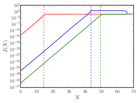
Figure 7: The evolution of the non-minimal coupling function $J$ [as given by Eqs. (66) and (67)] that we had considered in the models described by the potentials (57), (58) and (LABEL:eq:pi2) has been plotted (in solid red, blue and green, respectively) as a function of the e-fold $N$. The onset of the ultra slow roll phase corresponds to the time when the first slow roll parameter starts to decrease rapidly. We have indicated the beginning of the ultra slow roll epoch (as dashed vertical lines of the corresponding color) in all these cases. Recall that, we had constructed coupling functions $J(\phi)$ so that they behave as $a^{2}$ during the initial slow roll phase. For such choices of $J(\phi)$, the coupling function does not seem to change appreciably (until very close to the end of inflation) after ultra slow has set in.

Let us now examine the corresponding situation in the helical case. In the case of the helical field, during the initial stage of slow roll inflation, when $n=2$, the electromagnetic modes ${\mathcal{A}}_{k}^{\sigma}$ are given by [cf. Eq. (20)]

$${\mathcal{A}}_{k}^{\sigma\mathrm{I}}(\eta)=\frac{1}{\sqrt{2\,k}}\,\mathrm{e}^{-\pi\,\sigma\,\gamma}\,W_{2\,i\,\sigma\,\gamma,\tfrac{5}{2}}(2\,i\,k\,\eta).$$ (75)

Since the coupling function $J$ hardly evolves after the onset of ultra slow roll, the electromagnetic modes during the second stage, say, ${\mathcal{A}}_{k}^{\sigma\mathrm{II}}$, can be expressed just as in Eq. (69) for the non-helical case. Moreover, the matching conditions continue to be given by Eqs. (70). However, we should clarify that the coefficients $\alpha_{k}$ and $\beta_{k}$ now depend on the polarization $\sigma$. The power spectra of the magnetic and electric fields at late times, i.e. when $(-k\,\eta_{\mathrm{e}})\ll 1$, can be obtained to be

$$\mathcal{P}_{{}_{\mathrm{B}}}(k) = \frac{H_{{}_{\mathrm{I}}}^{4}}{8\,\pi^{2}}\,\left(-k\,\eta_{\mathrm{e}}\right)^{4}\,\left(|\alpha_{k}^{+}+\beta_{k}^{+}|^{2}+|\alpha_{k}^{-}+\beta_{k}^{-}|^{2}\right),$$

$$\mathcal{P}_{{}_{\mathrm{E}}}(k) = \frac{H_{{}_{\mathrm{I}}}^{4}}{8\,\pi^{2}}\,\left(-k\,\eta_{\mathrm{e}}\right)^{4}\,\left(|\alpha_{k}^{+}-\beta_{k}^{+}|^{2}+|\alpha_{k}^{-}-\beta_{k}^{-}|^{2}\right).$$

On matching the modes at $\eta_{1}$, we obtain the coefficients $\alpha_{k}^{\sigma}$ and $\beta_{k}^{\sigma}$ to be

$$\alpha_{k}^{\sigma} = -\frac{\mathrm{e}^{-i\,k/k_{1}}\,\mathrm{e}^{-\pi\,\sigma\,\gamma}}{2\,(k/k_{1})}\,\biggl{[}2\,(i+\sigma\,\gamma)\,W_{2\,i\,\sigma\,\gamma,\tfrac{5}{2}}(-2\,i\,k/k_{1})$$ (77a)

$$-i\,W_{1+2\,i\,\sigma\,\gamma,\tfrac{5}{2}}(-2\,i\,k/k_{1})\biggr{]},$$

$$\beta_{k}^{\sigma} = -\frac{\mathrm{e}^{i\,k/k_{1}}\,\mathrm{e}^{-\pi\,\sigma\,\gamma}}{2\,(k/k_{1})}\,\biggl{[}2\,\left(-i-\frac{k}{k_{1}}-\sigma\,\gamma\right)$$

$$\times\,W_{2\,i\,\sigma\,\gamma,\tfrac{5}{2}}(-2\,i\,k/k_{1})+i\,W_{1+2\,i\,\sigma\,\gamma,\tfrac{5}{2}}(-2\,i\,k/k_{1})\biggr{]},$$

where, as earlier, we have set $k_{1}=-1/\eta_{1}$. In the limit $k/k_{1}\gg 1$, we find that $\alpha_{k}^{\sigma}\to 1$ and $\beta_{k}^{\sigma}\to 0$, as in the non-helical case. This suggests that the power spectra of both the electric and magnetic fields behave as $k^{4}$ in such a limit, which is indeed what we obtain numerically (see Figs. 5 and 6). Whereas, in the limit $k/k_{1}\ll 1$, we find that [84]

$$|\alpha_{k}^{\sigma}+\beta_{k}^{\sigma}|^{2} = \frac{9\,\left(1-\mathrm{e}^{-4\,\pi\,\sigma\,\gamma}\right)}{4\,\pi\,\sigma\,\gamma\,\left(1+5\,\gamma^{2}+4\,\gamma^{4}\right)}\,\left(\frac{k}{k_{1}}\right)^{-4},\quad$$ (78)

$$|\alpha_{k}^{\sigma}-\beta_{k}^{\sigma}|^{2} = \frac{9\,\sigma\,\gamma^{2}\,\left(1-\mathrm{e}^{-4\,\pi\,\sigma\,\gamma}\right)}{4\,\pi\,\gamma\,\left(1+5\,\gamma^{2}+4\,\gamma^{4}\right)}\,\left(\frac{k}{k_{1}}\right)^{-4},$$ (79)

and hence the spectra (76) reduce to the following forms:

$$\mathcal{P}_{{}_{\mathrm{B}}}(k) \simeq \frac{9\,H_{{}_{\mathrm{I}}}^{4}}{4\,\pi^{2}}\,f(\gamma)\,\left[\frac{a(\eta_{1})}{a(\eta_{\mathrm{e}})}\right]^{4},$$ (80a)

$$\mathcal{P}_{{}_{\mathrm{E}}}(k) \simeq \frac{9\,H_{{}_{\mathrm{I}}}^{4}}{4\,\pi^{2}}\,f(\gamma)\,\gamma^{2}\,\left[\frac{a(\eta_{1})}{a(\eta_{\mathrm{e}})}\right]^{4},$$ (80b)

where, recall that, $f(\gamma)$ is given by Eq. (28). Clearly, over large scales, the spectra of both the electric and magnetic fields are scale invariant as is expected in the helical case when $J\simeq a^{2}$ and the modes cross the Hubble radius during a regime of slow roll. Moreover, note that, as in the non-helical case, the onset of the ultra slow roll epoch leads to a suppression in the amplitudes of the power spectra on large scales by the factor of $[a(\eta_{1})/a(\eta_{\mathrm{e}})]^{4}$.

We have been able to understand the shape of the electromagnetic spectra arising in models involving an epoch of ultra slow roll inflation using analytical arguments. Let us now compare the numerical results for the amplitudes of the spectra over large scales with the analytical estimates in both the non-helical and helical cases. In the case of the ultra slow roll model described by the potential (58), we find that, when the pivot scale leaves the Hubble radius, the value of the Hubble parameter is $H_{{}_{\mathrm{I}}}=9.05\times 10^{-6}\,M_{{}_{\mathrm{Pl}}}$. The epoch of ultra slow roll inflation can be said to begin when the first slow roll parameter $\epsilon_{1}$ attains the maximum value (prior to the end of inflation) and begins to decrease rapidly thereafter. We find that, in the model of our interest here, ultra slow roll sets in about $22.4$ e-folds before the end of inflation. Also, the value of the wave number that equals $\sqrt{|J^{\prime\prime}/J|}$ at the onset of ultra slow roll inflation proves to be $k_{1}=2.2\times 10^{13}\,\mathrm{Mpc}^{-1}$. For these values, in the non-helical case, the analytical estimates we have obtained above lead to $\mathcal{P}_{{}_{\mathrm{B}}}(k)\simeq 10^{-60}\,M_{{}_{\mathrm{Pl}}}^{4}$ and $\mathcal{P}_{{}_{\mathrm{E}}}(k)\simeq 10^{-89}\,M_{{}_{\mathrm{Pl}}}^{4}$ at the pivot scale. Numerically, we have obtained the corresponding values to be $\mathcal{P}_{{}_{\mathrm{B}}}(k)\simeq 10^{-63}\,M_{{}_{\mathrm{Pl}}}^{4}$ and $\mathcal{P}_{{}_{\mathrm{E}}}(k)\simeq 10^{-84}\,M_{{}_{\mathrm{Pl}}}^{4}$. In the helical case, for $\gamma=1$, the analytical estimates lead to $\mathcal{P}_{{}_{\mathrm{B}}}(k)=\mathcal{P}_{{}_{\mathrm{E}}}(k)\simeq 10^{-57}\,M_{{}_{\mathrm{Pl}}}^{4}$ at the pivot scale. The corresponding numerical values turn out to be $\mathcal{P}_{{}_{\mathrm{B}}}(k)=\mathcal{P}_{{}_{\mathrm{E}}}(k)\simeq 10^{-60}\,M_{{}_{\mathrm{Pl}}}^{4}$.

Similarly, in the case of the second model of punctuated inflation described by the potential (LABEL:eq:pi2), we find that the value of the Hubble parameter at the time when the pivot scale exits the Hubble radius is $H_{{}_{\mathrm{I}}}=1.01\times 10^{-5}\,M_{{}_{\mathrm{Pl}}}$. Moreover, the onset of the ultra slow roll epoch occurs about $18.3$ e-folds prior to the end of inflation, which implies that $k_{1}\simeq 1.6\times 10^{14}\,\mathrm{Mpc}^{-1}$. According to the analytical estimates, in the non-helical case, these values lead to $\mathcal{P}_{{}_{\mathrm{B}}}(k)\simeq 10^{-53}\,M_{{}_{\mathrm{Pl}}}^{4}$ and $\mathcal{P}_{{}_{\mathrm{E}}}(k)\simeq 10^{-84}\,M_{{}_{\mathrm{Pl}}}^{4}$ at the pivot scale. Numerically, we obtain the corresponding values to be $\mathcal{P}_{{}_{\mathrm{B}}}(k)\simeq 10^{-50}\,M_{{}_{\mathrm{Pl}}}^{4}$ and $\mathcal{P}_{{}_{\mathrm{E}}}(k)\simeq 10^{-83}\,M_{{}_{\mathrm{Pl}}}^{4}$. In the case of the helical fields, when $\gamma=1$, the analytical estimates suggest that $\mathcal{P}_{{}_{\mathrm{B}}}(k)=\mathcal{P}_{{}_{\mathrm{E}}}(k)\simeq 10^{-50}\,M_{{}_{\mathrm{Pl}}}^{4}$ at the pivot scale, while the corresponding numerical values turn out to be $\mathcal{P}_{{}_{\mathrm{B}}}(k)=\mathcal{P}_{{}_{\mathrm{E}}}(k)\simeq 10^{-47}\,M_{{}_{\mathrm{Pl}}}^{4}$.

While the analytical estimates broadly match the numerical results, there arise differences of the order of $10^{3}$–$10^{5}$ in the values for the power spectra of the electromagnetic fields. These differences can be attributed to the coarseness of the analytical modeling and the fact that $J$ evolves to a certain extent as one approaches the end of inflation.

V.4.2 A closer look at the evolution of the modes at late times

In Fig. 7, we had plotted the evolution of the non-minimal coupling function in the ultra slow roll model and the two punctuated inflation models we have considered. We had found that, once the epoch of ultra slow roll begins, the coupling function $J$ hardly evolves. Based on such a behavior, we had assumed that $J^{\prime}$ and $J^{\prime\prime}$ were zero and had arrived at the analytical form for the modes ${\mathcal{A}}_{k}$ and, eventually, the power spectra of the electromagnetic fields. While the coupling function $J$ is almost a constant, one can show that it is not correct to set $J^{\prime}$ and $J^{\prime\prime}$ to zero in these scenarios. In Fig. 8, we have plotted the evolution of $|J^{\prime\prime}/J|$ in the three models.

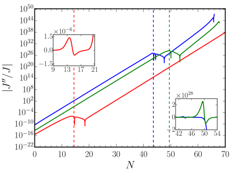
Figure 8: The evolution of the quantity $J^{\prime\prime}/J$ corresponding to the three coupling functions we had illustrated in the previous figure has been plotted as a function of e-fold $N$ (with the same choice of colors). The insets highlight the behavior of the quantity around the onset of the epoch of ultra slow roll. We find that $J^{\prime\prime}/J\propto\mathrm{e}^{2\,N}$ during the initial slow roll phase, as expected. It is clear $J^{\prime\prime}/J$ does not vanish once ultra slow roll inflation begins (indicated by the vertical lines). In fact, the quantity is almost a constant during the period of ultra slow roll and it actually grows (either as $\mathrm{e}^{2\,N}$ in the case of the first punctuated inflation model or as $\mathrm{e}^{5\,N/2}$ in the other two models) when the phase of ultra slow roll is complete and the first slow roll parameter begins to rise. We should also mention the fact that $J^{\prime\prime}/J$ can turn negative during these latter stages.

It is clear from the figure that the quantity does not vanish once ultra slow begins, as we have assumed earlier. Therefore, it seems that we need to revise our previous discussion.

One can expect that, since $J$ as well as $J^{\prime\prime}/J$ behave as $a^{2}$ during the initial slow roll phase, the power spectra over modes that leave the Hubble radius — to be precise, when $k=\sqrt{|J^{\prime\prime}/J|}$ — will be scale invariant. However, in the ultra slow roll and the second punctuated inflation models, once the epoch of ultra slow roll comes to an end, $J^{\prime\prime}/J$ behaves as $a^{5/2}$ (as illustrated in Fig. 8), while $J$ is a constant. Let us now focus on large wave numbers in these models over which, numerically, we find that the power spectra of the magnetic as well as electric fields behave as $k^{4}$. In these cases, at suitably early times when $k\gg\sqrt{|J^{\prime\prime}/J|}$, the Fourier modes of the non-helical vector potential [governed by Eq. (4)] can be written as

$${\mathcal{A}}_{k}^{\mathrm{I}}(\eta)=\frac{1}{\sqrt{2\,k}}\,\mathrm{e}^{-i\,k\,\eta}.$$ (81)

Also, since, $J$ is a constant, at late times when $k\ll\sqrt{|J^{\prime\prime}/J|}$, we can express the non-helical electromagnetic modes as

$${\mathcal{A}}_{k}^{\mathrm{II}}(\eta)=\frac{1}{\sqrt{2\,k}}\,\left[\alpha_{k}+\beta_{k}\,\eta\right],$$ (82)

where the coefficients $\alpha_{k}$ and $\beta_{k}$ are to be determined by matching the above solutions and their derivatives at the time $\eta_{k}$ corresponding to $k=\sqrt{|J^{\prime\prime}/J|}$. The coefficients $\alpha_{k}$ and $\beta_{k}$ can be easily obtained to be

$$\alpha_{k}=(1+i\,k\,\eta_{k})\,\mathrm{e}^{-i\,k\,\eta_{k}},\quad\beta_{k}=-i\,k\,\eta_{k}\,\mathrm{e}^{-i\,k\,\eta_{k}},$$ (83)

and hence, at late times, we have

$${\mathcal{A}}_{k}^{\mathrm{II}}(\eta)=\frac{1}{\sqrt{2\,k}}\,\left[1-i\,k\,(\eta-\eta_{k})\right]\,\mathrm{e}^{-i\,k\,\eta_{k}}.$$ (84)

Since $J$ is constant, this implies that the quantity $\sqrt{k}\,\bar{A}_{k}$ will have the same value at late times [i.e. when $(-k\,\eta_{\mathrm{e}})\ll 1$] for large wave numbers provided $(k\,\eta_{k})$ is small. We shall see below that $(k\,\eta_{k})$ is indeed small in the models of our interest. In Fig. 9, we have plotted the evolution of the electromagnetic modes at late times in the case of the ultra slow roll inflation model (58) for a range of wave numbers.

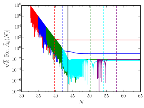
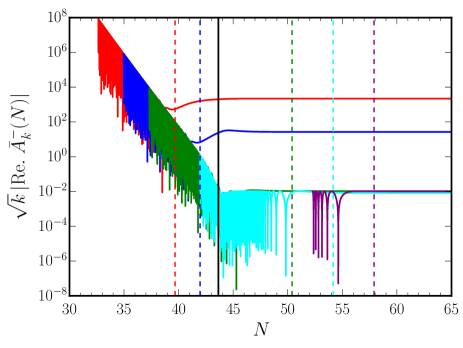
Figure 9: The evolution of the electromagnetic modes in the case of the ultra slow roll inflation model (58) has been plotted for the five choices of the wave numbers $k=(10^{12},10^{13},10^{14},10^{16},10^{18})\;\mathrm{Mpc}^{-1}$ (in red, blue, green, cyan and purple), respectively. We have worked with the coupling function (67a) and have plotted the evolution of the dominant real part of the quantity $\sqrt{k}\,|\bar{A}_{k}|$ in the non-helical case (on the left) and the quantity $\sqrt{k}\,|\bar{A}_{k}^{-}|$ in the helical case (on the right). We have also indicated the onset of the ultra slow roll epoch (as the solid vertical line in black) and the e-folds corresponding to the time $\eta_{k}$, i.e. when $k^{2}=|J^{\prime\prime}/J|$, for the different wave numbers (as dashed vertical lines, with the same choice of colors as the modes). It is clear that the amplitude of the electromagnetic modes freeze at late times. Importantly, we find that, for $k\gtrsim 10^{13}\,\mathrm{Mpc}^{-1}$, the late time values of the quantities $\sqrt{k}\,|\bar{A}_{k}|$ and $\sqrt{k}\,|\bar{A}_{k}^{-}|$ are the same for the different wave numbers, which points to the $k^{4}$ behavior for the spectrum of the magnetic field over small scales.

It is clear from the figure that, over large enough wave numbers for which $\eta_{k}$ occurs after the epoch of ultra slow roll, the quantity $\sqrt{k}\,|A_{k}|$ has the same amplitude at late times. This, in turn, implies that the power spectrum of the magnetic field will behave as $k^{4}$, which is what we obtain numerically.

Note that, because of the fact that the first slow roll parameter remains small until we approach close to the end of inflation, the de Sitter expression for the scale factor remains valid. As a result, on using the above form for the electromagnetic modes, we obtain the spectra of the magnetic and electric fields in the limit $(-k\,\eta_{\mathrm{e}})\ll 1$ to be

$$\mathcal{P}_{{}_{\mathrm{B}}}(k) = \frac{H_{{}_{\mathrm{I}}}^{4}}{4\,\pi^{2}}\,(-k\,\eta_{\mathrm{e}})^{4}\,\left(1+k^{2}\,\eta_{k}^{2}\right),$$ (85a)

$$\mathcal{P}_{{}_{\mathrm{E}}}(k) = \frac{H_{{}_{\mathrm{I}}}^{4}}{4\,\pi^{2}}\,(-k\,\eta_{\mathrm{e}})^{4}.$$ (85b)

While $\mathcal{P}_{{}_{\mathrm{E}}}(k)$ is independent of $\eta_{k}$ and evidently behaves as $k^{4}$ over large wave numbers, we need to determine $\eta_{k}$ in order to understand the shape of $\mathcal{P}_{{}_{\mathrm{B}}}(k)$. Since $J^{\prime\prime}/J\propto a^{5/2}$ at late times, on using the behavior of the scale factor in de Sitter, based on dimensional grounds, we can write $J^{\prime\prime}/J=(k_{\mathrm{t}}\,\eta^{5})^{-1/2}$, where $k_{\mathrm{t}}$ is a wave number. The quantity $k_{\mathrm{t}}$ needs to be determined from the numerical value of $J^{\prime\prime}/J$ at the end of the ultra slow roll phase. Hence, the condition $k^{2}=J^{\prime\prime}/J=(k_{\mathrm{t}}\,\eta_{k}^{5})^{-1/2}$ leads to $k^{2}\,\eta_{k}^{2}=(k/k_{\mathrm{t}})^{2/5}$. In the ultra slow roll and the second punctuated inflation models, we find that, for our choices of the coupling functions, $k_{\mathrm{t}}\simeq 10^{23}\,\mathrm{Mpc}^{-1}$, whereas the largest wave number of our interest is $k\simeq 10^{19}\,\mathrm{Mpc}^{-1}$. These imply that $(k^{2}\,\eta_{k}^{2})\lesssim 10^{-2}$. Therefore, we can expect $\mathcal{P}_{{}_{\mathrm{B}}}(k)$ to behave as $k^{4}$ over the wave numbers $10^{15}\,\mathrm{Mpc}^{-1}\lesssim k\lesssim 10^{19}\,\mathrm{Mpc}^{-1}$, which is what we observe numerically.

In retrospect, it should be clear that the approaches in the last two subsections yielded similar results for the behavior of the spectra at large wave numbers because of the fact that the modes ${\mathcal{A}}_{k}^{\mathrm{II}}$ as given by Eqs. (69) and (82) have the same amplitudes at late times.

VI Can the features be ironed out?

It is now interesting to examine whether the features in the spectra of the electromagnetic fields can be ironed out so that we arrive at nearly scale invariant spectra for the magnetic field. In this section, we shall discuss this possibility in the second Starobinsky model [cf. Eqs. (55) and (56)] that leads to features in the scalar power spectrum over the large scales.

Earlier, we had arrived at the spectra of the magnetic field in this model assuming that the coupling function was given by either $J_{+}(\phi)$ or $J_{-}(\phi)$ described by Eqs. (65). In order to remove the strong features that arise in the spectrum of the magnetic field, it seems reasonable to stitch together these two coupling functions in the following fashion:

$$J(\phi) = \frac{J_{1}}{2\,J_{0+}}\,\left[1+\mathrm{tanh}\left(\frac{\phi-\phi_{0}}{\Delta\phi_{1}}\right)\right]\,J_{+}(\phi)$$ (86)

$$+\,\frac{J_{1}}{2\,J_{0-}}\,\left[1-\mathrm{tanh}\left(\frac{\phi-\phi_{0}}{\Delta\phi_{1}}\right)\right]\,J_{-}(\phi),\quad$$

where $J_{1}$ is constant which is determined by the condition that $J(\phi)$ reduces to unity at the end of inflation and $\Delta\phi_{1}$ is another constant which we shall choose suitably. Note that, for a small enough $\Delta\phi_{1}$, the quantities within the square brackets (involving the hyperbolic tangent functions) in the above expression behave as step functions. It should then be evident that the above coupling function has been constructed in such a fashion that it is essentially described by $J_{+}(\phi)$ when $\phi>\phi_{0}$ and $J_{-}(\phi)$ when $\phi<\phi_{0}$. In Fig. 10, we have plotted the resulting spectra for the magnetic as well as electric fields obtained numerically in the non-helical and helical cases.

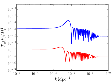
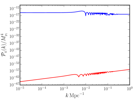
Figure 10: The spectra of the magnetic (on the left) and electric (on the right) fields arising for the choice of the coupling function (86) in the second Starobinsky model (56) have been plotted for both the non-helical (in red) and helical (in blue) cases. As before, we have set $n=2$ and $\gamma=1$ when computing the spectra. Note that, with the new coupling function, the strong features have disappeared and we are left with relatively smaller features that can be expected to be consistent with the current constraints. Evidently, the burst of oscillations that remain in the spectra occurs because of the departure from slow roll as the field crosses the point $\phi_{0}$.

As can be seen from the figure, there arise two nearly scale invariant regions in the power spectra of the magnetic field (and in the case of the helical electric field), with a burst of oscillations in between. Clearly, the scale invariant parts correspond to the evolution of the field over the two linear parts of the potential and the oscillations arise as the deviations from slow roll occur when the field crosses $\phi_{0}$. Thus, in a model involving a strong departure from slow roll, with a suitable choice of the coupling function, we have been able to arrive at electromagnetic spectra that do not lead to significant backreaction and can also be largely consistent with the current constraints. However, we should stress the fact that it has been achieved only at the severe cost of an extremely fine tuned non-minimal coupling function.

VII Conclusions

A nearly scale invariant primordial scalar power spectrum, as is generated in slow roll inflationary models, is remarkably consistent with the CMB data [50, 85]. However, it has been repeatedly noticed that certain features in the scalar power spectrum can improve the fit to the data. Such features are often generated by considering potentials that induce departures from slow roll inflation [51, 52, 53, 54, 55, 56, 57, 58, 59, 60, 61, 62, 63].

Magnetic fields are generated during inflation by breaking the conformal invariance of the electromagnetic action. In this work, we have investigated the effects of deviations from slow roll on the spectra of the electromagnetic fields generated during inflation. Specifically, we have considered a class of inflationary models which allow transient deviations from slow roll and, as a result, generate localized features in the scalar power spectrum. When the electromagnetic fields are coupled to the scalar curvature, we found that it proves to be challenging to obtain nearly scale invariant magnetic fields of the desired shapes and strengths even in slow roll inflation. In contrast, this is easy to achieve when the electromagnetic field is coupled non-minimally to the inflaton, provided we work with model-dependent coupling functions. Therefore, we focused on situations wherein the electromagnetic field is coupled to the inflaton and evaluated the spectra of non-helical as well as helical electromagnetic fields in non-trivial scenarios involving deviations from slow roll. We found that, when strong departures from slow roll arise, apart from generating features in the scalar power spectrum, quite generically, these deviations also led to features in the spectra of electromagnetic fields. Moreover, in certain scenarios, it is also possible that the strengths of the magnetic fields are considerably suppressed on large scales. While it seems possible to remove the strong features in the spectra of the electromagnetic fields allowing us to arrive at nearly scale invariant spectra of required strengths, it is achieved at the terrible cost of extreme fine-tuning. In summary, if future observations confirm the presence of strong features in the primordial scalar power spectrum and, if the electromagnetic fields are to be generated by coupling them to the inflaton that is responsible for these features, then there seems to arise a severe challenge in being able to produce magnetic fields of the desired shape and strength in single field models of inflation. We are currently exploring possible ways of overcoming the challenge.

There are a couple of related points we wish to clarify before we conclude. As we have stressed earlier, in this work, we have focused on a domain wherein backreaction due to the electromagnetic fields is negligible [35, 36]. Another interesting aspect of generating electromagnetic fields during inflation is that they can induce non-adiabatic pressure perturbations which can source the adiabatic scalar perturbations on super-Hubble scales (in this context, see, for instance, Refs. [103, 79, 36]). This additional contribution can lead to distinguishable features in the CMB both at the level of the power spectrum as well as non-Gaussianities. However, for most of the models we have considered in this work, since the strength of generated magnetic fields over CMB scales is relatively weak, the effects arising from the induced curvature perturbations can be expected to be negligible. Nevertheless, it seems important to investigate these effects more closely in non-trivial scenarios involving departures from slow roll inflation We are also presently examining these issues.

Appendix A The electromagnetic spectral indices in slow roll inflation

In this appendix, we shall derive the spectral indices of the non-helical magnetic and electric fields, viz. $n_{{}_{\mathrm{B}}}$ and $n_{{}_{\mathrm{E}}}$, in the slow roll approximation.

Given the form $J=[a(\eta)/a(\eta_{\mathrm{e}})]^{n}$ for the non-minimal coupling function [cf. Eq. (6)], one finds that

$$\frac{J^{\prime\prime}}{J}=\mathcal{H}^{2}\,\left(n^{2}+n-n\,\epsilon_{1}\right),$$ (87)

where $\epsilon_{1}=-\dot{H}/H^{2}$ is the first slow roll parameter, and we should emphasize that this relation is exact. In the slow roll approximation, one can express the conformal Hubble parameter as [87, 88, 89, 90, 91, 92, 93, 94, 95, 96, 97]

$$\mathcal{H}=\frac{a^{\prime}}{a}\simeq-\frac{1}{(1-\epsilon_{1})\,\eta}.$$ (88)

so that, at the first order in the slow roll parameter $\epsilon_{1}$, we have

$$\frac{J^{\prime\prime}}{J}\simeq\frac{1}{\eta^{2}}\,\left[n^{2}+n+(2\,n^{2}+n)\,\epsilon_{1}\right].$$ (89)

In such a case, the solution to Eq. (4) that satisfies the Bunch-Davies initial conditions is given by

$${\mathcal{A}}_{k}(\eta)=\sqrt{-\frac{\pi\,\eta}{4}}\,\mathrm{e}^{i\,[\nu+(1/2)]\,\pi/2}\,H^{(1)}_{\nu}(-k\,\eta),$$ (90)

where, as we had mentioned earlier, $H_{\nu}^{(1)}(z)$ is the Hankel function of the first kind. For $\epsilon_{1}\ll 1$, at the first order in the slow roll parameter, the index $\nu$ is given by

$$\nu\simeq\left(n+\frac{1}{2}\right)+n\,\epsilon_{1}.$$ (91)

Note that, when $\epsilon_{1}=0$, the above solution reduces to the de Sitter solution (7), as required. Since we are eventually interested in the case $n=2$, for convenience, we shall assume that $\nu>1$. In such a case, we find that the power spectra of the magnetic and electric fields evaluated at late times can be expressed as

$$\mathcal{P}_{{}_{\mathrm{B}}}(k)\propto k^{5-2\,\nu},\quad\mathcal{P}_{{}_{\mathrm{E}}}(k)\propto k^{7-2\,\nu},$$ (92)

which correspond to the spectral indices of

$$n_{{}_{\mathrm{B}}}=4-2\,n\,(1+\epsilon_{1}),\quad n_{{}_{\mathrm{E}}}=6-2\,n\,(1+\epsilon_{1}).$$ (93)

For $n=2$, these correspond to $n_{{}_{\mathrm{B}}}=-4\,\epsilon_{1}$ and $n_{{}_{\mathrm{E}}}=2-4\,\epsilon_{1}$.

Since $0<\epsilon_{1}\ll 1$, the above results imply that, for $n=2$, in the non-helical case, the spectrum of the magnetic field should be red in slow roll inflation. However, on closer inspection of Fig. 2, we find that the spectrum of the magnetic field is red in the case of the quadratic potential (40), but is mildly blue in the cases of the small field model (43) and the first Starobinsky model (46), which lead to slow roll inflation. This can be attributed to the fact that the coupling functions (42), (45) and (48) do not exactly mimic the coupling function $J=[a(\eta)/a(\eta_{\mathrm{e}})]^{n}$. In the case of the quadratic potential, for the choice of the coupling function (42), we find that the quantity $J^{\prime\prime}/J$ can be expressed as

$$\frac{J^{\prime\prime}}{J} = a^{2}\,H^{2}\,\biggl{[}\frac{n^{2}\,H^{2}}{m^{2}}\,(3\,\epsilon_{1}-\epsilon_{1}^{2})-n\,\epsilon_{1}$$ (94)

$$+\,\frac{n\,H}{m}\,\left(3\,\epsilon_{1}-\epsilon_{1}^{2}\right)^{1/2}\,\left(1-\epsilon_{1}+\frac{\epsilon_{2}}{2}\right)\biggr{]}.$$

We should mention that no approximations have been made in arriving at this expression. It does not seem possible to express the quantity $J^{\prime\prime}/J$ purely in terms of the slow roll parameters. For $n=2$, if we make use of the expression (88) for the conformal Hubble parameter $\mathcal{H}$, we obtain that

$$\frac{J^{\prime\prime}}{J} = \frac{1}{\eta^{2}}\biggl{\{}\frac{1}{(1-\epsilon_{1})^{2}}\,\biggl{[}\frac{4\,H^{2}}{m^{2}}\,(3\,\epsilon_{1}-\epsilon_{1}^{2})-2\,\epsilon_{1}$$ (95)

$$+\,\frac{2\,H}{m}\,\left(3\,\epsilon_{1}-\epsilon_{1}^{2}\right)^{1/2}\,\left(1-\epsilon_{1}+\frac{\epsilon_{2}}{2}\right)\biggr{]}\biggr{\}}.\quad$$

We should clarify that, while the quantity within the square brackets in this expression is an exact one, the conformal Hubble parameter has been evaluated in the slow roll approximation. Clearly, in such a case, the solution to the electromagnetic vector potential can be written in terms of the Hankel function as in Eq. (90). The index $\nu$ can be determined by equating the quantity within the curly brackets in the above expression for $J^{\prime\prime}/J$ to $\nu^{2}-(1/4)$. At the time when the pivot scale leaves the Hubble radius, for the choice of the parameters we have worked with, we find that $\nu=2.513$. Since $2\,\nu>5$, the spectrum of the magnetic field exhibits a red tilt for our choice of the coupling function in the case of the quadratic potential [cf. Eq. (92)].

We find that, in general, the quantity $J^{\prime\prime}/J$ can be expressed as

$$\frac{J^{\prime\prime}}{J}=a^{2}\,H^{2}\,\mu_{{}_{\mathrm{B}}}^{2}(N),$$ (96)

where $\mu_{{}_{\mathrm{B}}}(N)$ is given by

$$\mu_{{}_{\mathrm{B}}}^{2}(N)=\frac{J_{NN}}{J}+(1-\epsilon_{1})\,\frac{J_{N}}{J},$$ (97)

with $J_{N}={\mathrm{d}}J/{\mathrm{d}}N$ and $J_{NN}={\mathrm{d}}^{2}J/{\mathrm{d}}^{2}N$. If we make use of the conformal Hubble parameter in the slow roll approximation [cf. Eq. (88)], then, we can write

$$\frac{J^{\prime\prime}}{J}=\frac{1}{\eta^{2}}\,\frac{\mu_{{}_{\mathrm{B}}}^{2}(N)}{\left(1-\epsilon_{1}\right)^{2}},$$ (98)

which implies that $\nu^{2}-(1/4)=\mu_{{}_{\mathrm{B}}}^{2}/(1-\epsilon_{1})^{2}$, with $\mu_{{}_{\mathrm{B}}}$ and $\epsilon_{1}$ evaluated, say, when the pivot scale leaves the Hubble radius. Note that, one obtains a strictly scale invariant spectrum for the magnetic field when $\mu_{{}_{\mathrm{B}}}^{2}/(1-\epsilon_{1})^{2}=6$, which corresponds to $2\,\nu=5$. For our choice of the coupling function, in the case of the quadratic potential, at the time the pivot scale leaves the Hubble radius, we find that $\mu_{{}_{\mathrm{B}}}^{2}/(1-\epsilon_{1})^{2}=6.068$, which leads to $\nu=2.513$ that we mentioned above. In the cases of the small field and the first Starobinsky models, for the choices of the coupling functions (45) and (48), we find that, when the pivot scale exits the Hubble radius, $\mu_{{}_{\mathrm{B}}}^{2}/(1-\epsilon_{1})^{2}=5.935$ and $5.939$ which correspond to $\nu=2.487$ and $2.488$, respectively. Since, $2\,\nu<5$, we obtain magnetic field spectra with blue tilts in these two cases.

References

- Grasso and Rubinstein [2001] D. Grasso and H. R. Rubinstein, Phys. Rept. 348, 163 (2001), arXiv:astro-ph/0009061 .
- Giovannini [2004] M. Giovannini, Int. J. Mod. Phys. D 13, 391 (2004), arXiv:astro-ph/0312614 .
- Brandenburg and Subramanian [2005] A. Brandenburg and K. Subramanian, Phys. Rept. 417, 1 (2005), arXiv:astro-ph/0405052 .
- Kulsrud and Zweibel [2008] R. M. Kulsrud and E. G. Zweibel, 71, 0046091 (2008), arXiv:0707.2783 [astro-ph] .
- Subramanian [2010] K. Subramanian, Astron. Nachr. 331, 110 (2010), arXiv:0911.4771 [astro-ph.CO] .
- Kandus et al. [2011] A. Kandus, K. E. Kunze, and C. G. Tsagas, Phys. Rept. 505, 1 (2011), arXiv:1007.3891 [astro-ph.CO] .
- Widrow et al. [2012] L. M. Widrow, D. Ryu, D. R. G. Schleicher, K. Subramanian, C. G. Tsagas, and R. A. Treumann, Space Sci. Rev. 166, 37 (2012), arXiv:1109.4052 [astro-ph.CO] .
- Durrer and Neronov [2013] R. Durrer and A. Neronov, Astron. Astrophys. Rev. 21, 62 (2013), arXiv:1303.7121 [astro-ph.CO] .
- Subramanian [2016] K. Subramanian, Rept. Prog. Phys. 79, 076901 (2016), arXiv:1504.02311 [astro-ph.CO] .
- Vachaspati [2020] T. Vachaspati 10.1088/1361-6633/ac03a9 (2020), arXiv:2010.10525 [astro-ph.CO] .
- Neronov and Vovk [2010] A. Neronov and I. Vovk, Science 328, 73 (2010), arXiv:1006.3504 [astro-ph.HE] .
- Tavecchio et al. [2010] F. Tavecchio, G. Ghisellini, L. Foschini, G. Bonnoli, G. Ghirlanda, and P. Coppi, Mon. Not. Roy. Astron. Soc. 406, L70 (2010), arXiv:1004.1329 [astro-ph.CO] .
- Dolag et al. [2011] K. Dolag, M. Kachelriess, S. Ostapchenko, and R. Tomas, Astrophys. J. Lett. 727, L4 (2011), arXiv:1009.1782 [astro-ph.HE] .
- Dermer et al. [2011] C. D. Dermer, M. Cavadini, S. Razzaque, J. D. Finke, J. Chiang, and B. Lott, Astrophys. J. Lett. 733, L21 (2011), arXiv:1011.6660 [astro-ph.HE] .
- Vovk et al. [2012] I. Vovk, A. M. Taylor, D. Semikoz, and A. Neronov, Astrophys. J. Lett. 747, L14 (2012), arXiv:1112.2534 [astro-ph.CO] .
- Taylor et al. [2011] A. Taylor, I. Vovk, and A. Neronov, Astron. Astrophys. 529, A144 (2011), arXiv:1101.0932 [astro-ph.HE] .
- Takahashi et al. [2012] K. Takahashi, M. Mori, K. Ichiki, and S. Inoue, Astrophys. J. Lett. 744, L7 (2012), arXiv:1103.3835 [astro-ph.CO] .
- Paoletti and Finelli [2019] D. Paoletti and F. Finelli, JCAP 11, 028, arXiv:1910.07456 [astro-ph.CO] .
- Barrow and Tsagas [2008] J. D. Barrow and C. G. Tsagas, Phys. Rev. D 77, 107302 (2008), [Erratum: Phys.Rev.D 77, 109904 (2008)], arXiv:0803.0660 [astro-ph] .
- Barrow and Tsagas [2011] J. D. Barrow and C. G. Tsagas, Mon. Not. Roy. Astron. Soc. 414, 512 (2011), arXiv:1101.2390 [astro-ph.CO] .
- Adamek et al. [2012] J. Adamek, C. de Rham, and R. Durrer, Mon. Not. Roy. Astron. Soc. 423, 2705 (2012), arXiv:1110.2019 [gr-qc] .
- Shtanov and Sahni [2013] Y. Shtanov and V. Sahni, JCAP 01, 008, arXiv:1211.2168 [astro-ph.CO] .
- [23] D. Yamauchi, T. Fujita, and S. Mukohyama, JCAP 03, 031, arXiv:1402.2784 [astro-ph.CO] .
- Ade et al. [2016] P. A. R. Ade et al. (Planck), Astron. Astrophys. 594, A19 (2016), arXiv:1502.01594 [astro-ph.CO] .
- Turner and Widrow [1988] M. S. Turner and L. M. Widrow, Phys. Rev. D 37, 2743 (1988).
- Ratra [1992] B. Ratra, Astrophys. J. Lett. 391, L1 (1992).
- Bamba and Yokoyama [2004] K. Bamba and J. Yokoyama, Phys. Rev. D 69, 043507 (2004), arXiv:astro-ph/0310824 .
- Bamba and Sasaki [2007] K. Bamba and M. Sasaki, JCAP 02, 030, arXiv:astro-ph/0611701 .
- Martin and Yokoyama [2008] J. Martin and J. Yokoyama, JCAP 01, 025, arXiv:0711.4307 [astro-ph] .
- Bamba and Odintsov [2008] K. Bamba and S. D. Odintsov, JCAP 04, 024, arXiv:0801.0954 [astro-ph] .
- Demozzi et al. [2009] V. Demozzi, V. Mukhanov, and H. Rubinstein, JCAP 08, 025, arXiv:0907.1030 [astro-ph.CO] .
- Bamba et al. [2021a] K. Bamba, E. Elizalde, S. D. Odintsov, and T. Paul, JCAP 04, 009, arXiv:2012.12742 [gr-qc] .
- Bamba et al. [2021b] K. Bamba, S. D. Odintsov, T. Paul, and D. Maity, (2021b), arXiv:2107.11524 [gr-qc] .
- Watanabe et al. [2009] M.-a. Watanabe, S. Kanno, and J. Soda, Phys. Rev. Lett. 102, 191302 (2009), arXiv:0902.2833 [hep-th] .
- Kanno et al. [2009] S. Kanno, J. Soda, and M.-a. Watanabe, JCAP 12, 009, arXiv:0908.3509 [astro-ph.CO] .
- Markkanen et al. [2017] T. Markkanen, S. Nurmi, S. Rasanen, and V. Vennin, JCAP 06, 035, arXiv:1704.01343 [astro-ph.CO] .
- Anber and Sorbo [2006] M. M. Anber and L. Sorbo, JCAP 10, 018, arXiv:astro-ph/0606534 .
- Durrer et al. [2011] R. Durrer, L. Hollenstein, and R. K. Jain, JCAP 03, 037, arXiv:1005.5322 [astro-ph.CO] .
- Caprini and Sorbo [2014] C. Caprini and L. Sorbo, JCAP 10, 056, arXiv:1407.2809 [astro-ph.CO] .
- Chowdhury et al. [2018] D. Chowdhury, L. Sriramkumar, and M. Kamionkowski, JCAP 10, 031, arXiv:1807.07477 [astro-ph.CO] .
- Sharma et al. [2018] R. Sharma, K. Subramanian, and T. R. Seshadri, Phys. Rev. D 97, 083503 (2018), arXiv:1802.04847 [astro-ph.CO] .
- Giovannini [2021a] M. Giovannini, Class. Quant. Grav. 38, 135018 (2021a), arXiv:2012.14720 [gr-qc] .
- Giovannini [2021b] M. Giovannini, (2021b), arXiv:2106.14927 [hep-th] .
- Gorbar et al. [2021a] E. V. Gorbar, K. Schmitz, O. O. Sobol, and S. I. Vilchinskii, (2021a), arXiv:2109.01651 [hep-ph] .
- Gorbar et al. [2021b] E. V. Gorbar, K. Schmitz, O. O. Sobol, and S. I. Vilchinskii, (2021b), arXiv:2111.04712 [hep-ph] .
- Zucca et al. [2017] A. Zucca, Y. Li, and L. Pogosian, Phys. Rev. D 95, 063506 (2017), arXiv:1611.00757 [astro-ph.CO] .
- Sutton et al. [2017] D. R. Sutton, C. Feng, and C. L. Reichardt, Astrophys. J. 846, 164 (2017), arXiv:1702.01871 [astro-ph.CO] .
- Paoletti et al. [2019] D. Paoletti, J. Chluba, F. Finelli, and J. A. Rubino-Martin, Mon. Not. Roy. Astron. Soc. 484, 185 (2019), arXiv:1806.06830 [astro-ph.CO] .
- Minoda et al. [2021] T. Minoda, K. Ichiki, and H. Tashiro, JCAP 03, 093, arXiv:2012.12542 [astro-ph.CO] .
- Akrami et al. [2020] Y. Akrami et al. (Planck), Astron. Astrophys. 641, A10 (2020), arXiv:1807.06211 [astro-ph.CO] .
- Contaldi et al. [2003] C. R. Contaldi, M. Peloso, L. Kofman, and A. D. Linde, JCAP 07, 002, arXiv:astro-ph/0303636 .
- Sinha and Souradeep [2006] R. Sinha and T. Souradeep, Phys. Rev. D 74, 043518 (2006), arXiv:astro-ph/0511808 .
- Powell and Kinney [2007] B. A. Powell and W. H. Kinney, Phys. Rev. D 76, 063512 (2007), arXiv:astro-ph/0612006 .
- Jain et al. [2009] R. K. Jain, P. Chingangbam, J.-O. Gong, L. Sriramkumar, and T. Souradeep, JCAP 01, 009, arXiv:0809.3915 [astro-ph] .
- Jain et al. [2010] R. K. Jain, P. Chingangbam, L. Sriramkumar, and T. Souradeep, Phys. Rev. D 82, 023509 (2010), arXiv:0904.2518 [astro-ph.CO] .
- Hazra et al. [2010] D. K. Hazra, M. Aich, R. K. Jain, L. Sriramkumar, and T. Souradeep, JCAP 10, 008, arXiv:1005.2175 [astro-ph.CO] .
- Benetti [2013] M. Benetti, Phys. Rev. D 88, 087302 (2013), arXiv:1308.6406 [astro-ph.CO] .
- Hazra et al. [2014a] D. K. Hazra, A. Shafieloo, G. F. Smoot, and A. A. Starobinsky, Phys. Rev. Lett. 113, 071301 (2014a), arXiv:1404.0360 [astro-ph.CO] .
- Hazra et al. [2014b] D. K. Hazra, A. Shafieloo, G. F. Smoot, and A. A. Starobinsky, JCAP 08, 048, arXiv:1405.2012 [astro-ph.CO] .
- Chen et al. [2016a] X. Chen, P. D. Meerburg, and M. Münchmeyer, JCAP 09, 023, arXiv:1605.09364 [astro-ph.CO] .
- Chen et al. [2016b] X. Chen, C. Dvorkin, Z. Huang, M. H. Namjoo, and L. Verde, JCAP 11, 014, arXiv:1605.09365 [astro-ph.CO] .
- Ragavendra et al. [2020] H. Ragavendra, D. Chowdhury, and L. Sriramkumar, (2020), arXiv:2003.01099 [astro-ph.CO] .
- Antony and Jain [2021] A. Antony and S. Jain, (2021), arXiv:2110.06837 [astro-ph.CO] .
- Abbott et al. [2021] R. Abbott et al. (LIGO Scientific, Virgo), Astrophys. J. Lett. 913, L7 (2021), arXiv:2010.14533 [astro-ph.HE] .
- De Luca et al. [2020] V. De Luca, G. Franciolini, P. Pani, and A. Riotto, JCAP 06, 044, arXiv:2005.05641 [astro-ph.CO] .
- Jedamzik [2020] K. Jedamzik, JCAP 09, 022, arXiv:2006.11172 [astro-ph.CO] .
- Jedamzik [2021] K. Jedamzik, Phys. Rev. Lett. 126, 051302 (2021), arXiv:2007.03565 [astro-ph.CO] .
- Franciolini et al. [2021] G. Franciolini, V. Baibhav, V. De Luca, K. K. Y. Ng, K. W. K. Wong, E. Berti, P. Pani, A. Riotto, and S. Vitale, (2021), arXiv:2105.03349 [gr-qc] .
- Garcia-Bellido and Ruiz Morales [2017] J. Garcia-Bellido and E. Ruiz Morales, Phys. Dark Univ. 18, 47 (2017), arXiv:1702.03901 [astro-ph.CO] .
- Ballesteros and Taoso [2018] G. Ballesteros and M. Taoso, Phys. Rev. D 97, 023501 (2018), arXiv:1709.05565 [hep-ph] .
- Germani and Prokopec [2017] C. Germani and T. Prokopec, Phys. Dark Univ. 18, 6 (2017), arXiv:1706.04226 [astro-ph.CO] .
- Dalianis et al. [2019] I. Dalianis, A. Kehagias, and G. Tringas, JCAP 01, 037, arXiv:1805.09483 [astro-ph.CO] .
- Bhaumik and Jain [2020] N. Bhaumik and R. K. Jain, JCAP 01, 037, arXiv:1907.04125 [astro-ph.CO] .
- Ashoorioon et al. [2021] A. Ashoorioon, A. Rostami, and J. T. Firouzjaee, JHEP 07, 087, arXiv:1912.13326 [astro-ph.CO] .
- Ragavendra et al. [2021] H. V. Ragavendra, P. Saha, L. Sriramkumar, and J. Silk, Phys. Rev. D 103, 083510 (2021), arXiv:2008.12202 [astro-ph.CO] .
- Dalianis and Kritos [2021] I. Dalianis and K. Kritos, Phys. Rev. D 103, 023505 (2021), arXiv:2007.07915 [astro-ph.CO] .
- Byrnes et al. [2012] C. T. Byrnes, L. Hollenstein, R. K. Jain, and F. R. Urban, JCAP 03, 009, arXiv:1111.2030 [astro-ph.CO] .
- Ferreira et al. [2013] R. J. Ferreira, R. K. Jain, and M. S. Sloth, JCAP 10, 004, arXiv:1305.7151 [astro-ph.CO] .
- Ferreira et al. [2014] R. J. Ferreira, R. K. Jain, and M. S. Sloth, JCAP 06, 053, arXiv:1403.5516 [astro-ph.CO] .
- Shtanov [2019] Y. Shtanov, JCAP 10, 008, arXiv:1902.05894 [astro-ph.CO] .
- Shtanov and Pavliuk [2020] Y. Shtanov and M. Pavliuk, JCAP 08, 042, arXiv:2004.00947 [astro-ph.CO] .
- Chowdhury et al. [2019] D. Chowdhury, L. Sriramkumar, and M. Kamionkowski, JCAP 01, 048, arXiv:1807.05530 [astro-ph.CO] .
- Gradshteyn et al. [2014] I. S. Gradshteyn, I. M. Ryzhik, D. Zwillinger, and V. Moll, Table of integrals, series, and products; 8th ed. (Academic Press, Amsterdam, 2014).
- [84] W. R. Inc., Mathematica, Version 12.3.1, champaign, IL, 2021.
- Ade et al. [2021] P. A. R. Ade et al. (BICEP/Keck), Phys. Rev. Lett. 127, 151301 (2021), arXiv:2110.00483 [astro-ph.CO] .
- Ng et al. [2015] K.-W. Ng, S.-L. Cheng, and W. Lee, Chin. J. Phys. 53, 110105 (2015), arXiv:1409.2656 [astro-ph.CO] .
- Mukhanov et al. [1992] V. F. Mukhanov, H. A. Feldman, and R. H. Brandenberger, Phys. Rept. 215, 203 (1992).
- Martin [2004] J. Martin, Braz. J. Phys. 34, 1307 (2004), arXiv:astro-ph/0312492 .
- Martin [2005] J. Martin, Lect. Notes Phys. 669, 199 (2005), arXiv:hep-th/0406011 .
- Bassett et al. [2006] B. A. Bassett, S. Tsujikawa, and D. Wands, Rev. Mod. Phys. 78, 537 (2006).
- Baumann and Peiris [2009] D. Baumann and H. V. Peiris, Adv. Sci. Lett. 2, 105 (2009), arXiv:0810.3022 [astro-ph] .
- Sriramkumar [2009] L. Sriramkumar, Curr. Sci. 97, 868 (2009), arXiv:0904.4584 [astro-ph.CO] .
- Kinney [2009] W. H. Kinney, (2009), arXiv:0902.1529 [astro-ph.CO] .
- Baumann [2009] D. Baumann, in Theoretical Advanced Study Institute in Elementary Particle Physics: Physics of the Large and the Small (2009) arXiv:0907.5424 [hep-th] .
- Sriramkumar [2012] L. Sriramkumar, On the generation and evolution of perturbations during inflation and reheating, in Vignettes in Gravitation and Cosmology, edited by L. Sriramkumar and T. R. Seshadri (World Scientific, Singapore, 2012).
- Linde [2014] A. Linde, in 100e Ecole d’Ete de Physique: Post-Planck Cosmology (2014) arXiv:1402.0526 [hep-th] .
- Martin [2016] J. Martin, Astrophys. Space Sci. Proc. 45, 41 (2016), arXiv:1502.05733 [astro-ph.CO] .
- Hazra et al. [2013] D. K. Hazra, L. Sriramkumar, and J. Martin, JCAP 05, 026, arXiv:1201.0926 [astro-ph.CO] .
- Adams et al. [2001] J. A. Adams, B. Cresswell, and R. Easther, Phys. Rev. D 64, 123514 (2001), arXiv:astro-ph/0102236 .
- Starobinsky [1992] A. A. Starobinsky, JETP Lett. 55, 489 (1992).
- Martin and Sriramkumar [2012] J. Martin and L. Sriramkumar, JCAP 01, 008, arXiv:1109.5838 [astro-ph.CO] .
- Byrnes et al. [2019] C. T. Byrnes, P. S. Cole, and S. P. Patil, JCAP 06, 028, arXiv:1811.11158 [astro-ph.CO] .
- Bonvin et al. [2012] C. Bonvin, C. Caprini, and R. Durrer, Phys. Rev. D 86, 023519 (2012), arXiv:1112.3901 [astro-ph.CO] .