Distinguishing between $\Lambda$CDM and $f(R)$ gravity models using halo ellipticity correlations in simulations

Abstract

There is a growing interest in utilizing intrinsic alignment (IA) of galaxy shapes as a geometric and dynamical probe of cosmology. In this paper we present the first measurements of IA in a modified gravity model using the gravitational shear-intrinsic ellipticity correlation (GI) and intrinsic ellipticity-ellipticity correlation (II) functions of dark-matter halos from $f(R)$ gravity simulations. By comparing them with the same statistics measured in $\Lambda$CDM simulations, we find that the IA statistics in different gravity models show distinguishable features, with a trend similar to the case of conventional galaxy clustering statistics. Thus, the GI and II correlations are found to be useful in distinguishing between the $\Lambda$CDM and $f(R)$ gravity models. More quantitatively, IA statistics enhance detectability of the imprint of $f(R)$ gravity on large scale structures by $\sim 40\%$ when combined with the conventional halo clustering in redshift space. We also find that the correlation between the axis ratio and orientation of halos becomes stronger in $f(R)$ gravity than that in $\Lambda$CDM. Our results demonstrate the usefulness of IA statistics as a probe of gravity beyond a consistency test of $\Lambda$CDM and general relativity.

1 Introduction

The origin of the cosmic acceleration has been one of the most profound mysteries for decades (Weinberg et al., 2013). Many studies have explored it by considering dark energy as a source of the cosmic acceleration. Modifying the law of gravity at cosmological scales is an alternative way to explain the acceleration (Wang & Steinhardt, 1998; Linder, 2005). Conventionally, galaxy clustering observed in redshift surveys has been extensively exploited for this purpose (e.g., Guzzo et al., 2008; Reyes et al., 2010; Okumura et al., 2016).

Intrinsic alignment (IA) of galaxy shapes, originally focused as a contaminant to gravitational lensing signals (Croft & Metzler, 2000; Heavens et al., 2000; Hirata & Seljak, 2004; Mandelbaum et al., 2006; Hirata et al., 2007; Okumura et al., 2009; Okumura & Jing, 2009; Blazek et al., 2011; Troxel & Ishak, 2015; Tonegawa & Okumura, 2022), has been drawing attention as a new dynamical and geometric probe of cosmology (e.g., Chisari & Dvorkin, 2013; Okumura et al., 2019; Taruya & Okumura, 2020; Kurita et al., 2021; Okumura & Taruya, 2021; Reischke et al., 2022). However, such a possibility has been explored merely by forecast studies or numerical simulations based on the $\Lambda$CDM model. Thus, we still do not know how the observed IA looks like in gravity models beyond general relativity (GR).

In this paper, we present the first measurements of IA statistics of dark-matter halos in modified gravity using N-body simulations of the $f(R)$ gravity model. We then show that the IA statistics are indeed useful to tighten the constraint on gravity models by combining with the conventional galaxy clustering statistics.

This paper is organized as follows. In Section 2, we briefly review the statistics of IA used in this paper. Section 3 describes N-body simulations under the $\Lambda$CDM and $f(R)$ gravity models. In Section 4, we present measurements of the halo clustering and alignment statistics. We investigate how well one can improve the distinguishability between the $\Lambda$CDM and $f(R)$ gravity models by considering the IA statistics in section 5. Our conclusions are given in Section 6.

2 Intrinsic alignment statistics

This section provides a brief description of the three-dimensional alignment statistics following Okumura & Taruya (2020). In this paper, we measure all the statistics in redshift space, and thus the halo overdensity field $\delta_{h}$ below is sampled in redshift space and suffers from redshift-space distortions (RSD Kaiser, 1987).

To begin with, orientations of halos or galaxies projected onto the sky are quantified by the two-component ellipticity, given as

$$\gamma_{(+,\times)}(\boldsymbol{x})=\frac{1-q^{2}}{1+q^{2}}(\cos(2\theta),\sin(2\theta)),$$ (1)

where $\theta$, defined on the plane normal to the line-of-sight, is the angle between the major axis projected onto the celestial sphere and the projected separation vector pointing to another object, $q$ is the minor-to-major axis ratio on the projected plane ($0\leq q\leq 1$).

In this paper, together with the halo density correlation function, $\xi_{hh}$, abbreviated as the GG correlation, we study two types of IA statistics, the intrinsic ellipticity (II) correlation functions, $\xi_{+}$ and $\xi_{-}$ (Croft & Metzler, 2000; Heavens et al., 2000), and the gravitational shear-intrinsic ellipticity (GI) correlation functions, $\xi_{h+}$ (Hirata & Seljak, 2004). These IA statistics are concisely defined as

$$\xi_{X}(\boldsymbol{r})=\langle[1+\delta_{h}(\boldsymbol{x}_{1})][1+\delta_{h}(\boldsymbol{x}_{2})]W_{X}(\boldsymbol{x}_{1},\boldsymbol{x}_{2})\rangle,$$ (2)

where $X=\{h+,+,-\}$ and ${\bf r}={\bf x}_{2}-{\bf x}_{1}$. The GI and II correlation functions are characterized by the function $W_{X}(\boldsymbol{x}_{1},\boldsymbol{x}_{2})$: $W_{h+}(\boldsymbol{x}_{1},\boldsymbol{x}_{2})=\gamma_{+}(\boldsymbol{x}_{2})$ and $W_{\pm}(\boldsymbol{x}_{1},\boldsymbol{x}_{2})=\gamma_{+}(\boldsymbol{x}_{1})\gamma_{+}(\boldsymbol{x}_{2})\pm\gamma_{\times}(\boldsymbol{x}_{1})\gamma_{\times}(\boldsymbol{x}_{2})$ for the GI and II correlation functions, respectively. For the II correlation, when we specifically refer to $\xi_{+}$ and $\xi_{-}$, they are abbreviated as the II($+$) and II($-$) correlations, respectively. Throughout this paper, we assume the distant-observer approximation so that $\hat{\boldsymbol{x}}_{1}=\hat{\boldsymbol{x}}_{2}\equiv\hat{\boldsymbol{x}}$, where a hat denotes a unit vector.

3 $f(R)$ gravity simulations

In $f(R)$ gravity theories, we replace the Ricci scalar $R$ in the Einstein-Hilbert action by some general function of $R$, $f(R)$, to mimic the effect of the cosmological constant $\Lambda$ (Starobinsky, 1980; De Felice & Tsujikawa, 2010; Nojiri & Odintsov, 2011). We adopt the functional form of $f(R)$ introduced by Hu & Sawicki (2007), where the deviation of the law of gravity from GR is characterized by $f_{R0}\equiv df(R)/dR|_{z=0}$.

We perform $N$-body simulations under the $\Lambda$CDM model and $f(R)$ gravity and study the difference of the alignment statistics measured from them. The cosmological N-body simulations have been run with ECOSMOG code (Li et al., 2012b). Every simulation in our paper consists of $512^{3}$ particles in a cubic box with the side length being $L=316h^{-1}\mathrm{Mpc}$. The initial condition of the simulation is generated with the 2LPTic code using second-order Lagrangian perturbation theory (Crocce et al., 2006). We set the initial redshift to $z=50$ and mainly work with the simulation outputs at $z=0$. Note that the same initial condition has been used for both of $\Lambda$CDM model and $f(R)$ gravity runs. Each simulation assumes the following cosmological parameters consistent with the measurement of the cosmic microwave background by Planck Collaboration et al. (2016): the total matter density $\Omega_{m}=0.3156$, the baryon density $\Omega_{b}=0.0492$, the cosmological constant $\Omega_{\Lambda}=0.6844$, the present-day Hubble parameter $H_{0}=67.27\,\mathrm{km/s/Mpc}$, the spectral index of initial curvature perturbations $n_{s}=0.9645$, and the amplitude of initial perturbations at $k=0.05\,\mathrm{Mpc}^{-1}$ being $A_{s}=2.2065\times 10^{-9}$. For the $f(R)$ gravity run, we choose the value of $f_{R0}$ as $|f_{R0}|=10^{-5}$ and set the functional form of $f(R)\propto R/(R+\mathrm{const})$. It is worth noting that the present-day linear mass variance smoothed at $8\,h^{-1}\mathrm{Mpc}$, referred to as $\sigma_{8}$, are set to 0.831 and 0.883 for the $\Lambda$CDM and $f(R)$ gravity runs, respectively.

From the simulation outputs, we identify dark matter halos with a phase-space halo finder of ROCKSTAR (Behroozi et al., 2013). In this paper, we use the standard definition for the halo mass, $M_{200}$, defined by a sphere with a radius $r_{200}$ within which the enclosed average density is 200 times the mean mater density (Navarro et al., 1996). We then create the halo catalogs with the mass threshold of $M_{200}>10^{13}\,h^{-1}\,M_{\odot}$ for the $f(R)$ gravity run, which contain 18,055 and 8,481 halos at $z=0$ and $1$, respectively. Adopting the same mass threshold for the $\Lambda$CDM run leads to the lower number density, by $\lesssim 10\%$ (Schmidt et al., 2009; Li et al., 2012a). Thus, to avoid inducing spurious distinguishability between the $\Lambda$CDM and $f(R)$ gravity models due to the different abundances, we include halos slightly lighter than $10^{13}\,h^{-1}M_{\odot}$ so that the number density of halos in the two runs coincides. The lowest halo mass can be resolved with 485 particles in our simulation. Our halo sample does not include subhalos. The velocity of each halo is computed by the average particle velocity within the innermost 10% of the virial radius. The principle axes of each halo in a projected plane are computed by diagonalizing the second moments of the distribution of all the member particles projected on the celestial plane, $I_{ij}\propto\sum_{k}\Delta x^{i}_{k}\Delta x^{j}_{k}$, where $\Delta x_{k}^{i}$ is the $i$th spatial component of the vector $\Delta\boldsymbol{x}_{k}$, the difference between the positions of the halo center and $k$-th member particles, and the sum is over all the particles within the virial radius of the halo. The two ellipticity components of each halo, projected along the third axis for instance, are estimated as (Valdes et al., 1983; Miralda-Escude, 1991; Croft & Metzler, 2000)

$$\gamma_{(+,\times)}=\frac{1}{I_{11}+I_{22}}(I_{11}-I_{22},2I_{12}).$$ (3)

In measuring the redshift-space density field and the projected shape field, we rotate the simulation box and regard each direction along the three axes of the box as the line of sight. We thus have three realizations for each of the $\Lambda$CDM and $f(R)$ simulations, though they are not fully independent. Thus, in the following, all the quantities are averaged over the three projections.

Figure 1: Distributions of minor-to-major axis ratios of projected halo shapes for $\Lambda$CDM and $f(R)$ gravity simulation runs. The solid and dashed curves show the results at $z=0$ and $1$, respectively. Halos with $M>10^{13}\,h^{-1}\,M_{\odot}$ in the $f(R)$ gravity model are counted, and the lower mass threshold is adopted for $\Lambda$CDM halos to make the number densities equivalent with the former. The error bars shown only for the $f(R)$ gravity results represent the Poisson error.

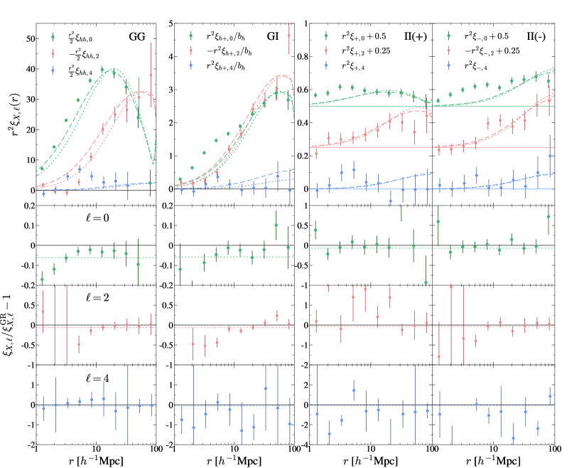
Figure 2: Multipole components of halo correlation functions in redshift space from $f(R)$ gravity mode at $z=0$, $\xi_{hh,\ell}$, $\xi_{h+,\ell}$, $\xi_{+,\ell}$, and $\xi_{-,\ell}$ from left to right panels in the first row. The second row shows the monopole correlation function from the $f(R)$ gravity model shown in the first row divided by that from the $\Lambda$CDM model. The third and fourth rows are similar with the second row but for the quadrupole and hexadecapole, respectively. The dotted horizontal lines are the best-fitting value of $A=\xi_{X,\ell}/\xi_{X,\ell}^{\rm GR}$, where $A_{\rm GG}=0.938$, $A_{\rm GI}=0.942$, and $A_{\rm II}=0.930$. The dotted curves in the top row show $\xi_{X,\ell}=A\xi_{X,\ell}^{\rm GR}$, where $\xi_{X,\ell}^{\rm GR}$ is calculated from the LA model for demonstration. For another demonstration, the dashed curves in the top row also show the LA model prediction with the matter power spectrum $P_{m}^{R}$ being calculated for the $f(R)$ gravity model using the MGCAMB code.

Fig. 1 shows the distributions of minor-to-major axis ratios of projected halo shapes at $z=0$ and 1 for $\Lambda$CDM and $f(R)$ gravity simulation runs. As mentioned above, the distributions are averaged over the three realizations. By comparing the two distributions at $z=1$, one can see that halo shapes in $f(R)$ gravity are more elongated than those in $\Lambda$CDM. It could be because more masses undergo infalling along the filaments into halo centers in $f(R)$ gravity than in $\Lambda$CDM. Toward $z=0$ where the structure growth becomes more nonlinear, the difference of the axis ratio distributions between $f(R)$ gravity and $\Lambda$CDM models becomes less prominent. These trends at $z=0$ and $1$ are totally consistent with the earlier finding of L’Huillier et al. (2017). In the following sections, we analyze the halo catalogs of $z=0$ only.

4 Correlation functions in $f(R)$ gravity

4.1 Correlation function measurements

Here we measure the GG, GI and II statistics in the $N$-body simulations. Since all these statistics have explicit angular dependences (Hamilton, 1992; Okumura & Taruya, 2020), we consider their multipole expansions in terms of the Legendre polynomials, $\mathcal{P}_{\ell}$,

$$\xi_{X,\ell}(r)=\frac{2\ell+1}{2}\int_{-1}^{1}\xi_{X}(\boldsymbol{r})\mathcal{P}_{\ell}(\mu_{\boldsymbol{r}})d\mu_{\boldsymbol{r}},$$ (4)

where $X=\{hh,h+,+,-\}$ and $\mu_{\boldsymbol{r}}=\hat{\bf r}\cdot\hat{\boldsymbol{x}}$ with a hat denoting a unit vector. In linear perturbation theory all the four correlation functions, $\xi_{X,\ell}$, have non-zero values only for $\ell=0,2$ and $4$. We thus consider only these three multipoles for each correlation function, and hence the number of the total statistics is $4\times 3=12$.

Our estimators for the multipoles, $\xi_{X,\ell}$, are expressed as (Okumura et al., 2020)

$$\xi_{X,\ell}(r)=\frac{2\ell+1}{2}\frac{1}{RR(r)}\sum\limits_{j,k|r=|\boldsymbol{x}_{k}-\boldsymbol{x}_{j}|}W_{X,jk}\mathcal{P}_{\ell}(\mu_{jk}),$$ (5)

where $RR$ is the pair counts from the random distribution, which can be analytically computed because we place the periodic boundary condition on the simulation box. For the GG, GI and II correlations, $W_{hh,jk}=1-\delta_{\ell 0}^{K}RR(r)/DD(r)$ , $W_{h+,jk}=\gamma_{+}(\boldsymbol{x}_{j})$, and $W_{\pm,jk}=\gamma_{+}(\boldsymbol{x}_{j})\gamma_{+}(\boldsymbol{x}_{k})\pm\gamma_{\times}(\boldsymbol{x}_{j})\gamma_{\times}(\boldsymbol{x}_{k})$, respectively, where $\gamma_{(+,\times)}$ is redefined relative to the separation vector $\boldsymbol{r}$ projected on the celestial sphere, $\delta_{\ell\ell^{\prime}}^{K}$ is the Kronecker delta and $DD(r)$ is the pair counts of halos at given separation $r$. Clustering of halos in $f(R)$ gravity has been investigated in literature using $N$-body simulations (Arnalte-Mur et al., 2017; Hernández-Aguayo et al., 2019; Alam et al., 2021; García-Farieta et al., 2021) and hydrodynamical simulations (Arnold & Li, 2019). On the other hand, we will present the first measurements of intrinsic alignments from modified gravity simulations.

From the left to right of the first row in Fig. 2, we show the multipole moments of the GG, GI, II($+$) and II($-$) correlation functions measured from the $f(R)$ gravity simulations at $z=0$. Since we have three realizations for each simulation run by rotating the simulation box (see Section 3), for each statistic we show the average over the three measurements. We adopt 10 logarithmically spaced bins in $r$ over $1<r<100[\,h^{-1}\,{\rm Mpc}]$. The data at the scales below and above this range are severely affected by the halo exclusion effect and cosmic variance, respectively. The second, third and last rows of Fig. 2 are respectively the monopole, quadrupole and hexadecapole moments from the $f(R)$ gravity simulation divided by those from the $\Lambda$CDM simulation, $\xi_{X,\ell}/\xi^{\rm GR}_{X,\ell}$. Note again that, all the correlation functions are measured in redshift space which are a direct observable in real galaxy surveys, and thus they are affected by RSD.

Since the number density in the $f(R)$ gravity model tends to be higher than that in the GR model, halos in $f(R)$ gravity are less biased than those in $\Lambda$CDM with the same masses. To avoid this, we made our halo sample have the same number densities by lowering the mass threshold for the $\Lambda$CDM halos, as described in section 3. Nevertheless, the amplitude of the GG correlation in $f(R)$ gravity becomes lower than that in GR as seen in the lower panels of the leftmost column in Fig. 2, confirming the earlier finding that halos in $f(R)$ gravity tend to be less biased than those in $\Lambda$CDM (e.g., Alam et al., 2021).

Similarly to the GG correlation, the three multipoles of the GI correlation in the $f(R)$ gravity model shows a negative deviation from those in $\Lambda$CDM. Note that the non-zero hexadecapole comes from the RSD effect (Okumura & Taruya, 2020). Since the II($+$) and II($-$) correlation functions are noisier than the GI correlation function, as is known for the $\Lambda$CDM case, it is harder to see the difference in the II correlation. Nevertheless, for the monopole and quadrupole moments one can see the same trend that the amplitude in $f(R)$ gravity is smaller than that in $\Lambda$CDM, due to the fact that the amplitude of IA, often characterized by $b_{K}$ (see equation 8), is positively correlated with the halo bias (e.g., Jing, 2002; Okumura et al., 2020; Akitsu et al., 2021; Kurita et al., 2021); more massive halos tend to be more strongly aligned with the large-scale structure.

4.2 Covariance matrix

To perform a reliable statistical analysis, it is crucial to construct an accurate covariance error matrix. One of the most robust ways to do this is to use $N$-body simulations to generate many mock catalogs. It is, however, computationally very expensive as we need to run more than hundreds of independent simulations. It is particularly impractical for the case of modified gravity simulations, since they are computationally even more expensive than standard $\Lambda$CDM simulations. We thus need to employ an alternative approach that is not so accurate as generating many mock catalogs based on $N$-body simulations.

In our analysis, we use a bootstrap-resampling technique (Barrow et al., 1984) to estimate a covariance error matrix for the measured statistics in $f(R)$ gravity simulations. With a given original halo catalog, we construct a new catalog by randomly choosing the same number of halos as the original catalog, allowing repetition. We repeat this process until we obtain the required number of bootstrap realizations, $N_{\rm bs}$. For the $k$th realization ($1\leq k\leq N_{\rm bs}$), we measure the correlation function multipoles, $\xi_{X,\ell}^{k}(r)$, where $X=\{hh,h+,+,-\}$ and $\ell=0,2,4$. Once again, $\xi_{X,\ell}^{k}$ is the average of the three measurements by rotating the simulation box for the $k$th realization.

Given the measurements of the correlation functions, their covariance matrix, ${\rm C}_{ij}^{X_{\ell}X^{\prime}_{\ell^{\prime}}}\equiv{\rm C}\left[\xi_{X,\ell}(r_{i}),\xi_{X^{\prime},\ell^{\prime}}(r_{j})\right]$ can be estimated as

$${\rm C}_{ij}^{X_{\ell}X^{\prime}_{\ell^{\prime}}}=\frac{1}{N_{\rm bs}-1}\sum\limits^{N_{\rm bs}}_{k} \left[\xi^{k}_{X,\ell}(r_{i})-\bar{\xi}_{X,\ell}(r_{i})\right]$$ (6)

$$\times\left[\xi^{k}_{X^{\prime},\ell^{\prime}}(r_{j})-\bar{\xi}_{X^{\prime},\ell^{\prime}}(r_{j})\right],$$

where $\bar{\xi}_{X,\ell}$ is the average of $\xi_{X,\ell}^{k}$ over $N_{\rm bs}$ realizations, $\bar{\xi}_{X,\ell}=N_{\rm bs}^{-1}\sum^{N_{\rm bs}}_{k=1}\xi_{X,\ell}^{k}$. Since the number of bins of each statistic is 10, the size of the full covariance becomes $120\times 120$. In this work, we choose $N_{\rm bs}=500$ to avoid the covariance matrix being singular. The obtained full covariance matrix normalized by the diagonal elements, ${\rm C}_{ij}/({\rm C}_{ii}\cdot{\rm C}_{jj})^{1/2}$, is shown in Fig. 3. The diagonal components, ${\rm C}_{ii}^{1/2}$, are shown as the errorbars of our statistics in Fig. 2.

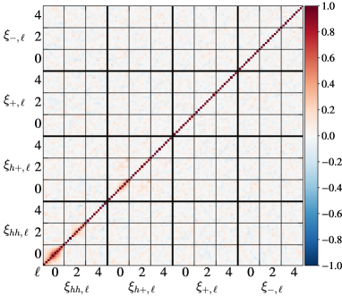
Figure 3: The $120\times 120$ normalized covariance matrix of the 12 correlation function multipoles, each of which has 10 logarithmic separation, $\xi_{X,\ell}(r)$, measured at $z=0$. We use 500 bootstrap realizations, and for every realization we measure the statistics three times by rotating the simulation box.

Note that the bootstrap method is known to underestimate the cosmic variance (Norberg et al., 2009). Thus, the constraints we will obtain in the next section become tighter than they should be. The purpose of this work is, however, to see how much adding the IA effect improves the distinguishability of different gravity models compared to the galaxy clustering analysis only, rather than the distinguishability itself. Thus, we do not expect that our conclusion is affected by the underestimation of the covariance matrix.

5 Results and discussion

5.1 Distinguishing gravity models with IA

Here we investigate how well one can improve the distinguishability between the $\Lambda$CDM and $f(R)$ gravity models by considering the IA statistics. For this purpose, we introduce a parameter $A$ which characterizes the difference between the given statistics $\xi_{X}$ of the two models, as $A\equiv\xi_{X}({\boldsymbol{r}})/\xi_{X}^{\rm GR}({\boldsymbol{r}})=\xi_{X,\ell}(r)/\xi_{X,\ell}^{\rm GR}(r)$, where $X=\{hh,h+,+,-\}$ and $\ell=\{0,2,4\}$, and constrain the parameter. We add subscripts to $A$ depending on which statistics to be used for the constraints, e.g., $A_{\rm GG}$, $A_{\rm GI}$ and $A_{\rm II}$ for the GG-, GI- and II-only analyses, respectively, and $A_{\rm GG+\rm GI+\rm II}$ for their combination. We adopt a simple $\chi^{2}$ statistic to constrain the parameter $A$ which is given by

$$\chi^{2}(A)=\sum\limits_{i,j,\ell,\ell^{\prime},X,X^{\prime}} \Delta^{X_{\ell}}_{i}\left({\rm C}^{-1}\right)_{ij}^{X_{\ell}X^{\prime}_{\ell^{\prime}}}\Delta^{X^{\prime}_{\ell^{\prime}}}_{j},$$ (7)

where $\Delta^{X_{\ell}}_{i}=\xi_{X,\ell}(r_{i})-A\xi^{\rm GR}_{X,\ell}(r_{i})$. The covariance of the correlation functions in $f(R)$ gravity, ${\rm C}_{ij}^{X_{\ell}X^{\prime}_{\ell^{\prime}}}$, is the $120\times 120$ matrix, and for the single-statistics analysis of the GG or GI correlation, the covariance is reduced to a $30\times 30$ submatrix, while the analysis of the II correlation, II($+$) and II($-$), needs the $60\times 60$ submatrix. Table LABEL:tab:table summarizes the degree of freedom for each choice of the statistics. Note that the constant model above is too simple and in reality the deviation of $A$ from unity is scale-dependent. We perform a qualitative investigation of the scale dependence using a simple model in $f(R)$ gravity in the next subsection. To properly take into account the scale dependence, however, the detailed modeling of IA statistics in modified gravity models is required. Furthermore, the amount of the deviation from unity is not necessarily equivalent between different statistics. Thus, we do not focus on the best-fitting values of $A$ but are rather interested in how well we can exclude the possibility of the correlation functions under the two models being equal, namely $A=1$, and whether the constraint gets tighter by combining the IA statistics with the clustering statistics.

Fig. 4 shows $\Delta\chi^{2}=\chi^{2}-\chi^{2}_{\min}$ as a function of $A$, where $\chi^{2}_{\min}$ is the minimized $\chi^{2}$ value with the best-fitting $A$. The black-dotted, yellow-dot-dashed and blue-long-dashed curves are the constraints from the GG, GI and II correlations, respectively. While the GG correlation gives the tightest constraint as expected, the GI and II correlations also provide meaningful constraints. The best-fitting parameter $A_{\rm GG}$ is shown as the horizontal lines in the second, third and fourth rows on the leftmost column of figure 2. Similarly, $A_{\rm GI}$ is shown on the second leftmost column and $A_{\rm II}$ is on the third and fourth columns.

Table 1: Summary of constraints on the ratio of the statistics between $f(R)$ gravity and $\Lambda$CDM models, $A=\xi_{X}/\xi_{X}^{\rm GR}$, at $z=0$. The second column represents the degree of freedom for each constraint.

Statistics	d.o.f. $\nu$	$\chi_{\min}^{2}$	$\Delta\chi^{2}(A=1)$ (C.L.)
GG	29	28.15	$15.2$ $(3.9\sigma)$
GI	29	42.9	$10.17$ $(3.19\sigma)$
II	59	41.87	$2.71$ $(1.6\sigma)$
GI$+$II	89	83.98	$20.35$ $(4.51\sigma)$
GG$+$GI$+$II	119	114.64	$31.74$ $(5.63\sigma)$

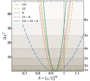
Figure 4: $\Delta\chi^{2}$ distribution for deviation parameter $A=\xi_{X}/\xi_{X}^{\rm GR}$ at $z=0$. The horizontal lines indicate confidence levels as shown in the right y-axis.

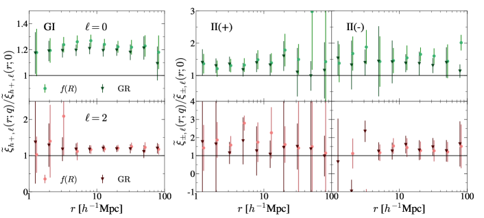
Figure 5: Left-hand set: ratios of normalized GI correlation functions with $q>0$ and $q=0$, $\widetilde{\xi}_{h+}(r;q)/\widetilde{\xi}_{h+}(r;0)$ (see Eq. (10) for the definition). Right-hand set: Same as the left-hand set but the ratios of normalized II correlation functions, $\widetilde{\xi}_{\pm}(r;q)/\widetilde{\xi}_{\pm}(r;0)$ (Eq. (11)). The upper and lower rows show results for the monopole and quadrupole moments, respectively. The deviation of the ratio from unity indicates the correlation between the halo ellipticity and orientation. The results for the $f(R)$ gravity and $\Lambda$CDM models are respectively shifted in the horizontally positive and negative directions for clarity.

We study how well one can improve the distinguishability between the $\Lambda$CDM and $f(R)$ gravity models by combining the IA statistics with the conventional clustering statistics. The constraint using the combination of GI and II correlations is shown as the red curve in Fig. 4. It is interesting to see that though the constraint from the conventional GG-correlation analysis is stronger and excludes the case of $\xi_{hh,\ell}=\xi_{hh,\ell}^{\rm GR}$ with $3.9\sigma$ C.L., one can achieve the meaningful constraint from GI+II ($4.51\sigma$). Once we combine all the statistics, namely 12 multipoles, the distinguishability reaches $5.63\sigma$. Note that the analysis is based on various assumptions and simplifications, and thus these numbers do not have much importance. Rather, the amount of the improvement ($\sim 40\%$) matters. All the obtained numerical values are summarized in table LABEL:tab:table.

5.2 Linear alignment model in $f(R)$ gravity

As a demonstration, we calculate the model prediction of the GG, GI and II correlations in $f(R)$ gravity using linear perturbation theory. In Fourier space, the halo density field in redshift space, $\delta_{h}(\boldsymbol{k})$, is linearly related to the underlying matter density field in real space, $\delta_{m}^{R}(\boldsymbol{k})$, via the Kaiser factor (Kaiser, 1987), $\delta_{h}(\boldsymbol{k})=(b_{h}+f\mu_{\boldsymbol{k}}^{2})\delta_{m}^{R}(\boldsymbol{k})$, where $\mu_{\boldsymbol{k}}=\hat{\boldsymbol{k}}\cdot\hat{\boldsymbol{x}}$ and $b_{h}$ is the linear halo bias. The superscript $R$ denotes a real-space quantity. The the growth rate, $f$, is defined as $f(z)=-d\ln{D(z)}/d\ln{(1+z)}$, with $D(z)$ being the growth factor. Different gravity models predict different values of $D(z)$ and $f(z)$. For the IA statistics, we adopt the linear alignment (LA) model (Catelan et al., 2001; Hirata & Seljak, 2004), which relates the ellipticity field linearly to the tidal gravitational field, described in Fourier space as

$$\gamma_{+}({\boldsymbol{k}})=b_{K}(k_{x}^{2}-k_{y}^{2})\delta_{m}^{R}({\boldsymbol{k}})/k^{2},$$ (8)

where $b_{K}$ is the shape bias parameter. Following Okumura & Taruya (2020) we introduce the expression,

$$\Xi_{\ell}(r)=\frac{1}{2\pi^{2}}\int_{0}^{\infty}k^{2-n}dkP_{m}^{R}(k)j_{\ell}(kr),$$ (9)

where $P_{m}^{R}(k)$ is the matter power spectrum in real space. We can then write all the IA statistics in the LA model in terms of $\Xi_{\ell}$, similarly to the case of the GG correlation (Hamilton, 1992; Okumura & Taruya, 2020). In the following, we compute $P_{m}^{R}(k)$ in two ways.

First, we use the CAMB code (Lewis et al., 2000) to compute $P_{m}^{R}(k)$ in the $\Lambda$CDM model and obtain the correlation functions, $\xi_{X,\ell}^{\rm GR}$. We then multiply it by the best-fitting value of $A$ obtained in Section 5.1 to have the prediction for $f(R)$ halos, $\xi_{X,\ell}=A\xi_{X,\ell}^{\rm GR}$. The bias parameter $b_{h}$ for the halos in $\Lambda$CDM is determined as $b_{h}^{\mathrm{GR}}=1.40$ by fitting the ratio of the GG correlation function to the matter correlation function $\xi_{m}^{R}=\Xi_{0}$, $b_{h}^{2}=\xi_{hh,0}^{R}/\xi_{m}^{R}$, to the measurement in the $\Lambda$CDM simulation on large scales. Similarly, $b_{K}$ is determined as $b_{K}^{\mathrm{GR}}=0.46$ by fitting $b_{K}^{2}=(15/8)\xi_{+,0}^{R}/\xi_{m}^{R}$.

Second, to take into account the scale dependence induced by the modification of gravity, we compute $P_{m}^{R}(k)$ directly in the $f(R)$ gravity model using the MGCAMB code (Zhao et al., 2009; Hojjati et al., 2011; Zucca et al., 2019). Similarly to the first case above, we determine the two biases, $b_{h}$ and $b_{K}$, by taking the ratios of the real-space correlation functions of halos measured from the $f(R)$ gravity simulation and the matter correlation function from the MGCAMB. They are determined as $b_{h}=1.34$ and $b_{K}=0.42$, lower than the values for the $\Lambda$CDM model, as expected. Different gravity models predict different values of the growth rate, $f(z)$. Furthermore, $f(z)$ can become scale dependent in modified gravity models, which arise from the effective gravitational constant (Narikawa & Yamamoto, 2010). Thus, the GG and GI correlation functions induce a further scale dependence due to $f(z)$ in the Kaiser factor.

In the top row of Fig. 2, we show the two LA predictions for halo statistics in $f(R)$ gravity explained above, one with the correlation function in $\Lambda$CDM multiplied by the best-fitting parameter $A$ obtained in section 5.1 (dotted curves), and another with the correlation function in $f(R)$ gravity directly computed using the MGCAMB code (dashed curves). Note that they are not fitting results of the LA model predictions: the parameter $A$ is constrained by the measured ratio of $\xi_{X,\ell}/\xi_{X,\ell}^{\rm GR}$ and the bias parameters are also determined by the simulation measurements. Nevertheless, we can see the LA model qualitatively explains the measured correlation functions of halos in $f(R)$ gravity. A close look at the small scale behavior of the correlation functions shows that the prediction based on the MGCAMB gives better agreement, particularly for the GG and GI correlation functions. It is important to note that the difference between the two model curves comes from the scale dependence of the growth factor $D(z)$ and its growth rate $f(z)$ which was not considered in section 5.1. Properly taking into account the effect will help improve the distinguishability between $\Lambda$CDM and $f(R)$ gravity models.

5.3 Correlation of halo shape and its orientation

Is there additional information encoded in the halo shape and orientation to distinguish different gravity models? To answer this, we consider normalized alignment statistics, which were introduced in Okumura & Jing (2009). The normalized GI and II correlation functions are defined as

$$\widetilde{\xi}_{h+}(\boldsymbol{r};q) =\left\langle\frac{1-q^{2}}{1+q^{2}}\right\rangle^{-1}\xi_{h+}(\boldsymbol{r};q),$$ (10)

$$\widetilde{\xi}_{\pm}(\boldsymbol{r};q) =\left\langle\frac{1-q^{2}}{1+q^{2}}\right\rangle^{-2}\xi_{\pm}(\boldsymbol{r};q),$$ (11)

where $\left\langle\frac{1-q^{2}}{1+q^{2}}\right\rangle$ is the value averaged over all the halos used for our analysis and $\xi_{X}(\boldsymbol{r};q)$ are the same as $\xi_{X}(\boldsymbol{r})$ in equation (2) but the dependence on $q$ is explicitly written. These normalized alignment statistics are useful because if there is no correlation between axis ratios and orientations, we simply expect $\widetilde{\xi}_{X}(\boldsymbol{r};q)=\widetilde{\xi}_{X}(\boldsymbol{r};0)$. Namely, even though the axis-ratio distributions were different between two models as shown in figure 1, it would not affect the distinguishability of gravity models if the normalized statistics were used.

In Fig. 5, we show the ratio of the multipoles, $\widetilde{\xi}_{X,\ell}(r;q)/\widetilde{\xi}_{X,\ell}(r;0)$. In all the statistics the ratios tend to be greater than unity, which implies that there are non-negligible correlations between the halo shape and orientation, consistent with the finding of Okumura & Jing (2009). Interestingly, for most of the statistics, the correlation is stronger in $f(R)$ gravity than in $\Lambda$CDM. This indicates that if properly modeled, considering the correlation between halo shapes and orientations potentially helps improve the distinguishability between $\Lambda$CDM and $f(R)$ gravity models. Blazek et al. (2011) studied the correlation in $\Lambda$CDM based on the LA model. We leave the study of the correlation between halo ellipticity and orientation for the $f(R)$ gravity model as future work.

6 Conclusions

In this paper, we have presented the first measurements of IA in a gravity model beyond GR using the two types of IA statistics, the GI and II correlation functions of halo shapes from $f(R)$ gravity simulations. By comparing them with the same statistics measured in $\Lambda$CDM simulations, we found that the IA statistics in different gravity models show distinguishable features, with a trend similar to the case of conventional galaxy clustering statistics. Quantitatively, IA statistics enhance detectability of the imprint of $f(R)$ gravity on large scale structures by $\sim 40\%$ when combined with the conventional halo clustering. We also found that the correlation between the axis ratio and orientation of halos becomes stronger in $f(R)$ gravity than that in $\Lambda$CDM.

Our constraints on different gravity models have been made assuming that the effect of the modified gravity on the clustering and IA statistics can be perfectly modeled. However, in the analysis of actual observations of IA, one needs to model the present statistics from linear to quasi non-linear scales. While there are several theoretical studies of IA beyond linear theory in GR (e.g., Blazek et al., 2019; Vlah et al., 2020), such predictions need to be carefully tested and extended to gravity models beyond GR. Furthermore, in real surveys, one observes shapes of galaxies, not of halos, thus misalignment between the major axes of galaxies and their host halos (Okumura et al., 2009) would degrade the detection significance of IA even in a modified gravity scenario. As a result, the distinguishability between different gravity models would be degraded compared to the results obtained in this paper. On the other hand, in this work we used only the amplitude of the multipole moments of the clustering and IA statistics, not the full shape of the underlying matter power spectrum which contains ample cosmological information but is more severely affected by the nonlinearities. Therefore, constraining power could eventually be either enhanced or suppressed. The more detailed and realistic analysis of clustering and IA statistics beyond a consistency test of GR will be performed in our future work.

Data Availability

The data underlying this article will be shared on reasonable request to the corresponding authors.

References

- Akitsu et al. (2021) Akitsu K., Li Y., Okumura T., 2021, J. Cosmology Astropart. Phys., 2021, 041
- Alam et al. (2021) Alam S., et al., 2021, J. Cosmology Astropart. Phys., 2021, 050
- Arnalte-Mur et al. (2017) Arnalte-Mur P., Hellwing W. A., Norberg P., 2017, MNRAS, 467, 1569
- Arnold & Li (2019) Arnold C., Li B., 2019, MNRAS, 490, 2507
- Barrow et al. (1984) Barrow J. D., Bhavsar S. G., Sonoda D. H., 1984, MNRAS, 210, 19P
- Behroozi et al. (2013) Behroozi P. S., Wechsler R. H., Wu H.-Y., 2013, ApJ, 762, 109
- Blazek et al. (2011) Blazek J., McQuinn M., Seljak U., 2011, J. Cosmology Astropart. Phys., 5, 10
- Blazek et al. (2019) Blazek J. A., MacCrann N., Troxel M. A., Fang X., 2019, Phys. Rev. D, 100, 103506
- Catelan et al. (2001) Catelan P., Kamionkowski M., Blandford R. D., 2001, MNRAS, 320, L7
- Chisari & Dvorkin (2013) Chisari N. E., Dvorkin C., 2013, J. Cosmology Astropart. Phys., 12, 029
- Crocce et al. (2006) Crocce M., Pueblas S., Scoccimarro R., 2006, MNRAS, 373, 369
- Croft & Metzler (2000) Croft R. A. C., Metzler C. A., 2000, Astrophys. J., 545, 561
- De Felice & Tsujikawa (2010) De Felice A., Tsujikawa S., 2010, Living Reviews in Relativity, 13, 3
- García-Farieta et al. (2021) García-Farieta J. E., Hellwing W. A., Gupta S., Bilicki M., 2021, Phys. Rev. D, 103, 103524
- Guzzo et al. (2008) Guzzo L., et al., 2008, Nature, 451, 541
- Hamilton (1992) Hamilton A. J. S., 1992, Astrophys. J. Lett., 385, L5
- Heavens et al. (2000) Heavens A., Refregier A., Heymans C., 2000, MNRAS, 319, 649
- Hernández-Aguayo et al. (2019) Hernández-Aguayo C., Hou J., Li B., Baugh C. M., Sánchez A. G., 2019, MNRAS, 485, 2194
- Hirata & Seljak (2004) Hirata C. M., Seljak U., 2004, Phys. Rev. D, 70, 063526
- Hirata et al. (2007) Hirata C. M., Mandelbaum R., Ishak M., Seljak U., Nichol R., Pimbblet K. A., Ross N. P., Wake D., 2007, MNRAS, 381, 1197
- Hojjati et al. (2011) Hojjati A., Pogosian L., Zhao G.-B., 2011, J. Cosmology Astropart. Phys., 2011, 005
- Hu & Sawicki (2007) Hu W., Sawicki I., 2007, Phys. Rev. D, 76, 064004
- Jing (2002) Jing Y. P., 2002, MNRAS, 335, L89
- Kaiser (1987) Kaiser N., 1987, MNRAS, 227, 1
- Kurita et al. (2021) Kurita T., Takada M., Nishimichi T., Takahashi R., Osato K., Kobayashi Y., 2021, MNRAS, 501, 833
- L’Huillier et al. (2017) L’Huillier B., Winther H. A., Mota D. F., Park C., Kim J., 2017, MNRAS, 468, 3174
- Lewis et al. (2000) Lewis A., Challinor A., Lasenby A., 2000, ApJ, 538, 473
- Li et al. (2012a) Li B., Zhao G.-B., Koyama K., 2012a, MNRAS, 421, 3481
- Li et al. (2012b) Li B., Zhao G.-B., Teyssier R., Koyama K., 2012b, J. Cosmology Astropart. Phys., 2012, 051
- Linder (2005) Linder E. V., 2005, Phys. Rev. D, 72, 043529
- Mandelbaum et al. (2006) Mandelbaum R., Hirata C. M., Ishak M., Seljak U., Brinkmann J., 2006, MNRAS, 367, 611
- Miralda-Escude (1991) Miralda-Escude J., 1991, ApJ, 370, 1
- Narikawa & Yamamoto (2010) Narikawa T., Yamamoto K., 2010, Phys. Rev. D, 81, 043528
- Navarro et al. (1996) Navarro J. F., Frenk C. S., White S. D. M., 1996, Astrophys. J., 462, 563
- Nojiri & Odintsov (2011) Nojiri S., Odintsov S. D., 2011, Phys. Rep., 505, 59
- Norberg et al. (2009) Norberg P., Baugh C. M., Gaztañaga E., Croton D. J., 2009, MNRAS, 396, 19
- Okumura & Jing (2009) Okumura T., Jing Y. P., 2009, ApJ, 694, L83
- Okumura & Taruya (2020) Okumura T., Taruya A., 2020, MNRAS, 493, L124
- Okumura & Taruya (2021) Okumura T., Taruya A., 2021, arXiv e-prints, p. arXiv:2110.11127
- Okumura et al. (2009) Okumura T., Jing Y. P., Li C., 2009, ApJ, 694, 214
- Okumura et al. (2016) Okumura T., et al., 2016, PASJ, 68, 38
- Okumura et al. (2019) Okumura T., Taruya A., Nishimichi T., 2019, Phys. Rev. D, 100, 103507
- Okumura et al. (2020) Okumura T., Taruya A., Nishimichi T., 2020, MNRAS, 494, 694
- Planck Collaboration et al. (2016) Planck Collaboration et al., 2016, A&A, 594, A13
- Reischke et al. (2022) Reischke R., Bosca V., Tugendhat T., Schäfer B. M., 2022, MNRAS, 510, 4456
- Reyes et al. (2010) Reyes R., Mandelbaum R., Seljak U., Baldauf T., Gunn J. E., Lombriser L., Smith R. E., 2010, Nature, 464, 256
- Schmidt et al. (2009) Schmidt F., Lima M. V., Oyaizu H., Hu W., 2009, Phys. Rev. D, 79, 083518
- Starobinsky (1980) Starobinsky A. A., 1980, Physics Letters B, 91, 99
- Taruya & Okumura (2020) Taruya A., Okumura T., 2020, ApJ, 891, L42
- Tonegawa & Okumura (2022) Tonegawa M., Okumura T., 2022, ApJ, 924, L3
- Troxel & Ishak (2015) Troxel M. A., Ishak M., 2015, Phys. Rep., 558, 1
- Valdes et al. (1983) Valdes F., Tyson J. A., Jarvis J. F., 1983, ApJ, 271, 431
- Vlah et al. (2020) Vlah Z., Chisari N. E., Schmidt F., 2020, J. Cosmology Astropart. Phys., 1, 025
- Wang & Steinhardt (1998) Wang L., Steinhardt P. J., 1998, ApJ, 508, 483
- Weinberg et al. (2013) Weinberg D. H., Mortonson M. J., Eisenstein D. J., Hirata C., Riess A. G., Rozo E., 2013, Phys. Rep., 530, 87
- Zhao et al. (2009) Zhao G.-B., Pogosian L., Silvestri A., Zylberberg J., 2009, Phys. Rev. D, 79, 083513
- Zucca et al. (2019) Zucca A., Pogosian L., Silvestri A., Zhao G.-B., 2019, JCAP, 05, 001