Wafer-level Variation Modeling for Multi-site RF IC Testing via Hierarchical Gaussian Process

Abstract

Wafer-level performance prediction has been attracting attention to reduce measurement costs without compromising test quality in production tests. Although several efficient methods have been proposed, the site-to-site variation, which is often observed in multi-site testing for radio frequency circuits, has not yet been sufficiently addressed. In this paper, we propose a wafer-level performance prediction method for multi-site testing that can consider the site-to-site variation. The proposed method is based on the Gaussian process, which is widely used for wafer-level spatial correlation modeling, improving the prediction accuracy by extending hierarchical modeling to exploit the test site information provided by test engineers. In addition, we propose an active test-site sampling method to maximize measurement cost reduction. Through experiments using industrial production test data, we demonstrate that the proposed method can reduce the estimation error to $1/19$ of that obtained using a conventional method. Moreover, we demonstrate that the proposed sampling method can reduce the number of the measurements by 97% while achieving sufficient estimation accuracy.

I Introduction

Large-scale integrated circuits (LSIs) are now embedded in every product to support the smooth functioning of our daily lives. In addition to automobiles, healthcare, and aerospace, which are directly related to human life, the LSIs are utilized in social infrastructure that supports our daily lives, such as computer networks, power transmission systems, and transportation control systems. However, with the spread of the LSIs, their reliability has become a crucial issue, and faulty LSIs that do not operate properly not only interrupt the services of the systems that include them but also lead to a serious impact on our society.

To guarantee the LSI reliability, multiple test items are tested and/or measured under various conditions during several stages of LSI manufacturing. With the increase in scale and multi-functionality of the LSIs, an increasing number of items need to be tested, leading to test cost inflation. Thus, it has become a serious problem because the test cost accounts for most of the LSI manufacturing cost.

Various test cost reduction methods have been proposed that apply data analytics, machine learning algorithms, and statistical methods [1, 2, 3]. In particular, the wafer-level characteristic modeling method based on a statistical algorithm is the most promising candidate that reduces the test cost, that is, measurement cost, without impairing the test quality [4, 5, 6, 7, 8, 9, 10, 11]. In these studies, a statistical modeling technique was used to predict the entire measurement on a wafer from a small number of sample measurements. Because the estimation eliminates the need for measurement, it not only reduces the cost of measurement but also can be used to reduce the number of test items and/or change the test limits, which is expected to improve the efficiency of adaptive testing [12, 13, 14, 15]. In [4], the expectation-maximization (EM) algorithm [16] was used to predict the measurement. In [5, 6, 7, 8], a statistical prediction method, called a virtual prove, based on compressed sensing [17, 18] was proposed. The Gaussian process (GP)-based method [19] provides more accurate prediction results [9, 11, 10]. The use of GP modeling has another side benefit. As it calculates the confidence of a prediction, the user can confirm whether the number and location of measurement samples are sufficient, which is a significant advantage from a practical viewpoint.

Most of these methods assume that the device characteristics on the wafer gradually change with wafer coordinates; however, this assumption does not hold for the measurement of radio frequency (RF) circuits under multi-site testing [20, 21, 22], in which a probe card is adapted to simultaneously probe multiple devices under test (DUTs). The contact of the probe card with the DUTs to be tested is called a touchdown. Moreover, the position of the needles in a touchdown is called a site. During the measurement of the RF circuit, a calibration circuit for impedance matching is added on the probe card, causing a much larger variation than the spatial variation due to its parasitic components, as shown in Fig. 1.

Figure 1(a) shows the histograms of the characteristics of an industrial RF circuits, which are fabricated using a 28 nm process technology, measured by a multi-site test with 16 sites per measurement in the first fabrication lot. The histograms are shown in different colors for each site. While low variance can be seen for each histogram, it is clear that there are significant differences between the histograms, that is, differences in sites. Most of the existing methods fail to model this measurement result because of the discontinuous change between the sites.

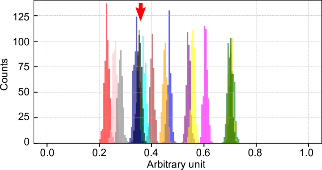
(a) First lot

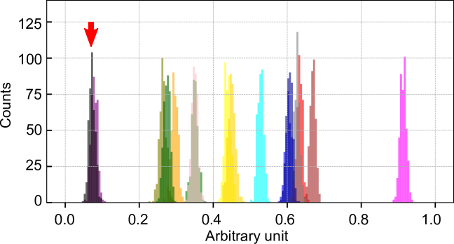
(b) Sixth lot

Figure 1: Histograms of measured characteristics of industrial RF circuit on a wafer, measured by multi-site testing with 16 sites. The histograms of each site are shown with different colors, i.e., 16 histograms are presented here. We can observe the significant variations in the histogram between sites. Furthermore, the locations of the black histograms are much different between the early and latest lots. The horizontal axis is expressed in arbitrary unit.

Only the work in [11] attempted to solve this issue of the discontinuous change. In [11], a two-step modeling method using $k$-means clustering [23] and the GP was proposed. In the first step, all dies on a wafer are explicitly measured, and then the $k$-means clustering algorithm is applied to divide the measurements into $k$ measurement groups, and the wafer coordinates are also clustered according to the $k$ measurement groups. In the second step, for the subsequently fabricated wafers, a GP is applied to each cluster individually. Because the spatial variation is modeled according to the partitioned magnitude of the measured value, even discontinuous changes can be reproduced accurately. In addition, there is a method [24] dealing with variations between the sites. In [24], in order to set outlier limits in a test, there is a method of eliminating the variation between sites by normalizing each site [24]. However, it is difficult to set the normalization constant appropriately in small sampling, and thus it is difficult to apply the site normalization to the wafer-level modeling.

However, this method relies heavily on the assumption that the $k$-means clustering results obtained from the first wafer are applicable to all subsequent lots. In fact, some site histograms drastically change in the latest fabrication lot, as shown in Fig. 1(b), which is the histograms in the sixth lot. For example, the highlighted black histogram should belong to a different cluster than that shown in Fig. 1(a) to achieve accurate prediction. While the possibility of recalibrating $k$-means clustering is described briefly, no specific solution has been provided in [11].

Herein, we propose a novel wafer-level spatial variation modeling method for RF circuits under multi-site testing. Test engineers usually have the site information of the probing; thus, we exploit it as a cluster in the proposed method, to predict spatial variation through the hierarchical GP modeling of each site. Therefore, the proposed method requires no clustering algorithm and no measurement corresponding to the first step. The use of site information is straightforward, but it is efficient under multi-site testing. Because the characteristics measured within one cluster have the same additional parasitic components of the calibration circuit, only spatial changes on the wafer are modeled; as a result, using the proposed method, accurate modeling can be achieved even across wafers. We also propose an active sampling method based on active learning [25] while considering the measurement of multi-site testing. Through the active sampling method utilizing the predictive variance of each site, the proposed method achieves optimal estimation with a small number of measured samples.

The main contributions of this work are summarized as follows:

• Hierarchical GP modeling using site information: Our method enables us to accurately model the spatial correlation on the wafer even for the measurement of RF circuits with the discontinuous changes for any lots by applying the GP separately to the correct clusters obtained from the site information.

• Active sampling algorithm under multi-site testing environment: We propose an efficient sampling algorithm based on the predictive variance of the estimation to determine the sample location.

• Comparison with the conventional method using industrial production data: We experimentally confirm that the assumption of the two-step modeling method [11], where the $k$-means clustering result can be applicable for subsequent wafers, does not hold in a more miniaturized fabrication process. We also demonstrate that the proposed method can reduce the prediction error to an average of $1/19.4$ compared to that obtained using the two-step modeling method.

• Thorough evaluation of the proposed active location selection algorithm: The experimental results also show that the proposed sampling method successfully reduces the number of touchdowns compared to the random sampling method without sacrificing the prediction accuracy. To the best of our knowledge, this is the first study to successfully demonstrate spatial variation modeling in a multi-site testing environment.

The remainder of this paper is organized as follows. Section II briefly explains GP, which plays a central role in the proposed method. In addition, we review the existing wafer-level spatial variation modeling based on the two-step approach [11], as a previous work. Then, in Section III, a hierarchical GP based on site information and an active sampling method for multi-site testing are proposed. The experimental results using industrial production test data of RF IC fabricated by a 28 nm process technology are presented in Section IV to quantitatively evaluate the effectiveness of the proposed method by comparing it with conventional methods. Finally, we conclude the paper in Section V.

II Preliminaries

II-A Gaussian process

First, we quickly review a GP [19], which is an integral part of the conventional method [11] and our method. The GP model is used for estimating the function $y=f(x)$ from the input variable $x$ to the output variable $y$, which is often used for regression. In the GP model, the function $f$ is assumed to follow a multidimensional normal distribution and is expressed as $f\sim\mathcal{N}(\bm{0},{\bm{Z}})$ using a kernel matrix ${\bm{Z}}$. One of its advantages is its ability to deal with nonlinear estimation problems. Another important advantage is the use of Bayesian inference [26]. Because the estimated function is obtained as a distribution of functions, not as a single function, the uncertainty of the estimation can be expressed as a predictive variance.

Algorithm 1 Gaussian process regression

1:Training dataset: $({\bm{X}}_{\rm train},{\bm{y}}_{\rm train})$, Test dataset: ${\bm{X}}_{\rm test}$, Kernel function: $f_{\rm kern}$

2:Mean and variance of predicted values: ${\bm{\mu}}=(\mu_{1},\mu_{2},\cdots,\mu_{M})$ and ${\bm{v}}=(v_{1},v_{2},\cdots,v_{M})$

3:for $n=1$ to $N$ do

4:     for $n^{\prime}=1$ to $N$ do

5:         Calculate $(n,n^{\prime})$-th element of a kernel matrix ${\bm{Z}}$ as $f_{\rm kern}({\bm{x}}_{n},{\bm{x}}_{n}^{\prime})$

6:     end for

7:end for

8:Calculate fitting parameters of $f_{\rm kern}$ to fit $({\bm{X}}_{\rm train},{\bm{y}}_{\rm train})$

9:for $m=1$ to $M$ do

10:     for $n=1$ to $N$ do

11:         Calculate $n$-th element of ${\bm{z}_{*}}$ as $f_{\rm kern}({\bm{x}}_{n},{\bm{x}^{*}}_{m})$

12:     end for

13:     ${\bm{z}_{**}}=f_{\rm kern}({\bm{x}^{*}}_{m},{\bm{x}^{*}}_{m})$

14:     Append $\mu_{m}={\bm{z}}^{T}_{*}{\bm{Z}}^{-1}{\bm{y}}_{\rm train}$ to ${\bm{\mu}}$

15:     Append $v_{m}={\bm{z}_{**}}-{\bm{Z}}^{-1}{\bm{z}}_{*}$ to ${\bm{v}}$

16:end for

The outline of a GP-based multiple regression is summarized in Algorithm 1. We consider $({\bm{X}}_{\rm train},{\bm{y}}_{\rm train})=\{({\bm{x}}_{1},y_{1}),({\bm{x}}_{2},y_{2}),\cdots,({\bm{x}}_{N},y_{N})\}$ and ${\bm{X}}_{\rm test}=({\bm{x}^{*}}_{1},{\bm{x}^{*}}_{2},\cdots,{\bm{x}^{*}}_{M})$ as the training and test datasets, respectively, where $M\gg N$. In addition, a kernel function $f_{\rm kern}$ is given as an input. Using the predicted model $f$ calculated based on $({\bm{X}}_{\rm train},{\bm{y}}_{\rm train})$, the algorithm returns the mean values and variances of the predicted ${\bm{y}^{*}}=(y^{*}_{1},y^{*}_{2},\cdots,y^{*}_{M})$ for ${\bm{X}}_{\rm test}$, ${\bm{\mu}}=(\mu_{1},\mu_{2},\cdots,\mu_{M})$ and ${\bm{v}}=(v_{1},v_{2},\cdots,v_{M})$.

In lines 1 to 5, the kernel matrix ${\bm{Z}}$ of the training dataset is calculated for each element of ${\bm{X}}_{\rm train}$ using the kernel function. Subsequently, in lines 7 to 14, the probability density function of the predicted $y^{*}_{m}$ corresponding to ${\bm{x}^{*}}_{m}$ is derived by modeling a multidimensional normal distribution as follows:

$$p(y^{*}_{m}|{\bm{x}^{*}}_{m},{\bm{X}}_{\rm train},{\bm{y}}_{\rm train})$$

$$= \mathcal{N}({\bm{z}}^{\mathrm{T}}_{*}{\bm{Z}}^{-1}{\bm{y}}_{\rm train},{\bm{z}_{**}}-{\bm{z}}^{\mathrm{T}}_{*}{\bm{Z}}^{-1}{\bm{z}}_{*}),$$

where ${\bm{z}}_{*}$ and ${\bm{z}}_{**}$ are the covariances between the training and test datasets and between the test datasets, respectively. As can be seen in Eq. (II-A), the mean value and variance of $y^{*}_{m}$ can be analytically derived. The expected values are used in the prediction, but the variances can also be used to confirm the uncertainty of the prediction.

There are several kernel functions, such as the linear, squared exponential, and Matérn kernels. For example, the radial basis function (RBF) kernel is as follows [27, 28]:

$$f_{\rm kern}({\bm{x}},{\bm{x}^{\prime}})=\theta_{1}\exp\left(-\frac{({\bm{x}}-{\bm{x}^{\prime}})^{2}}{\theta_{2}}\right),$$ (2)

where $\theta_{1}$ and $\theta_{2}$ are the fitting parameters calculated using an iterative optimization routine, as shown in line 6. As ${\bm{Z}}$ is a variance-covariance matrix, when ${\bm{x}}$ and ${\bm{x}^{\prime}}$ are close, $f_{\rm kern}({\bm{x}},{\bm{x}^{\prime}})$ becomes large and, as a result, $f({\bm{x}})$ and $f({\bm{x}^{\prime}})$ are also close.

The predictive mean $\bm{\mu}$ is used in wafer-level characteristics modeling. It can be expected that GP regression can be incorporated into the wafer-level spatial variation modeling in IC characteristics with high affinity, as the characteristics of adjacent dies on the wafer are similar because of the systematic components of process variation [29, 30].

II-B Related work

Owing to the intensive research on wafer-level spatial variation correlation modeling, the prediction accuracy of the spatial measurement variation has been improved, thereby, enabling the successful reduction of measurement costs in production tests [4, 5, 6, 7, 8, 9, 10, 11]. Among others, in [11], a two-step modeling approach has been proposed to handle the discontinuous effect induced by multi-site testing and reticle shot, etc., in wafer-level modeling.

The objective of the first step is to partition the wafer into $k$ groups, which reflect the $k$ levels of wafer measurement induced by discontinuous effects. For this purpose, the $k$-means algorithm is exploited as follows:

$${\bm{y}}=\{{\bm{y}}^{(1)},{\bm{y}}^{(2)},\cdots,{\bm{y}}^{(k)}\},$$ (3)

where ${\bm{y}}$ represents the vector of the measured characteristics of all the dies on the wafer. Consequently, ${\bm{X}}$ corresponding to ${\bm{y}}$ is partitioned as:

$${\bm{X}}=\{{\bm{X}}^{(1)},{\bm{X}}^{(2)},\cdots,{\bm{X}}^{(k)}\}.$$ (4)

Note that Eq. (4) indicates that the coordinates on the wafer are divided according to the measured characteristics. Once the $k$ clusters are identified, in the second step for subsequent wafers, the GP is applied to each cluster individually based on Algorithm 1. Because the changes in each ${\bm{y}}^{(k)}$ can be expected to be smooth, the GP regression will work successfully, and thus the two-step approach can handle discontinuous changes.

Note that determining the optimal $k$ is not trivial. Although several methods, such as silhouette value [31] and the elbow method [32], are well known to determine optimal $k$, in [11], $k$ is determined based on the following equation:

$$k=\mathop{\rm arg~{}max}\limits_{g}\,CH(g),$$ (5)

where $CH(g)$ is the Calinski and Harabasz index when $g$ clusters are considered [33].

However, the two-step modeling is not always applicable because it keeps using the $k$ clusters for subsequent wafers, assuming that the content of the clusters will not change for other wafers/lots. Because the experiment in [11] uses the industrial data fabricated using a relatively mature process technology, the assumption might hold true; in contrast, for our production data on immature process technology, the process is inapplicable, as shown in Fig. 1.

Another observation in Fig. 1 is shown in Fig 2. In this figure, the measured characteristics for each site are shown as functions of the lot ID from the first lot to the sixth lot. Here, the first wafer is used for each lot. The lines and shaded regions represent the mean and three standard deviations of each site, respectively. It can be seen that the distributions within the site are comparatively maintained up to the first two lots; however, they fluctuate greatly from the third lot. This suggests that the two-step modeling may work well up to the first two lots, whereas the clusters need to be recalibrated for the third and sixth lots, thus resulting in additional measurement costs. In addition, the early stage lots generally have low production yields, making it difficult to apply the two-step modeling method.

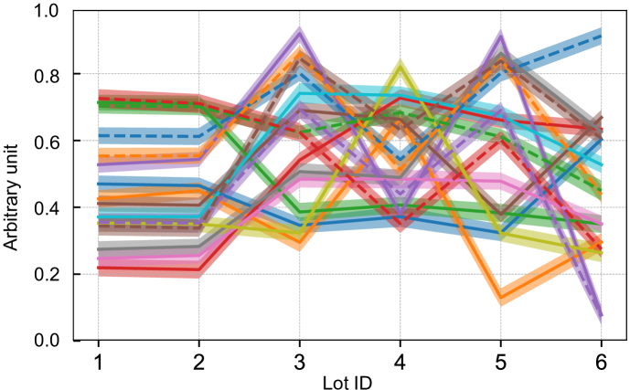
Figure 2: Measured characteristics of 16 sites from the first lot to the sixth lot. The solid lines and shaded regions represent the means and the three standard deviations of the variations, respectively. The vertical axis denotes arbitrary units.

III Wafer-level variation modeling for RF IC under multi-site testing

We propose a novel spatial variation model based on the site information provided by test engineers, which can give us the correct cluster without applying clustering algorithms. The GP-based prediction is hierarchically performed for each site cluster. Site-to-site variations are caused by parasitic components in the calibration circuit during multi-site testing. Ideally, they should be eliminated during measurement, which is impractical due to the design and manufacturing costs of the probe card. They also can be solved by considering them one at a time, but the benefits of multi-site testing cannot be obtained. The proposed method applies hierarchical GP modeling by clustering using site information and achieves highly accurate modeling while considering the actual measurement environment. As observed in Fig. 2, the measurements at the same site have a small deviation. The site-based hierarchical clustering can always be expected to be a good model without recalibration.

In addition, we propose an active sampling algorithm to achieve a small sampling ratio based on variance computed by GP-based regression in a multi-site testing environment. In contrast to all the existing studies that assume sampling one at a time, the proposed algorithm can effectively reduce the measurement cost.

III-A Modeling based on site-based hierarchical GP

Algorithm 2 Site-based hierarchical spatial variation modeling

1:${\bm{\mu}}$ and ${\bm{v}}$ Training dataset: $({\bm{X}}_{\rm train},{\bm{y}}_{\rm train})$ measured under multi-site testing, Test dataset: ${\bm{X}}_{\rm test}$, Kernel function: $f_{\rm kern}$, site information

2:Mean and variance of predicted values: ${\bm{\mu}}=(\mu_{1},\mu_{2},\cdots,\mu_{M})$ and ${\bm{v}}=(v_{1},v_{2},\cdots,v_{M})$

3:Cluster $({\bm{X}}_{\rm train},{\bm{y}}_{\rm train})$ and ${\bm{X}}_{\rm test}$ into $S$ groups according to the site information

4:for $s=1$ to $S$ do

5:     ${\bm{\mu}}^{(s)}$, ${\bm{v}}^{(s)}$ = gpr$\left(({\bm{X}}^{(s)}_{\rm train},{\bm{y}}^{(s)}_{\rm train}),{\bm{X}}^{(s)}_{\rm test},f_{\rm kern}\right)$

6:end for

7:Concatenate all ${\bm{\mu}}^{(s)}$ and ${\bm{v}}^{(s)}$ into ${\bm{\mu}}$ and ${\bm{v}}$

Algorithm 2 presents the proposed spatial correlation modeling through a site-based hierarchical GP in detail. We assume that the measurement is conducted by multi-site testing. The distinction from the conventional method is that the clustering is performed according to the site information in a single touchdown as listed in line 1, i.e., the conventional method needs to measure the characteristics of an entire wafer, whereas the proposed method requires no measurement for clustering. In Algorithm 2, $S$ represents the number of the sites in a single touchdown, and the training and test datasets are grouped into $S$ groups as follows:

$$({\bm{X}}_{\rm train},{\bm{y}}_{\rm train})=\{({\bm{X}}^{(1)}_{\rm train},{\bm{y}}^{(1)}_{\rm train}),({\bm{X}}^{(2)}_{\rm train},{\bm{y}}^{(2)}_{\rm train}),$$

$$\cdots,({\bm{X}}^{(S)}_{\rm train},{\bm{y}}^{(S)}_{\rm train})\}$$ (6)

and

$${\bm{X}}_{\rm test}=\{{\bm{X}}^{(1)}_{\rm test},{\bm{X}}^{(2)}_{\rm test},\cdots,{\bm{X}}^{(S)}_{\rm test}\},$$ (7)

respectively. The GP-based regression is performed individually by modeling each site hierarchically as listed in lines 2 to 4 based on the gpr function listed in Algorithm 1, where the mean and variance of the prediction for the test dataset are returned. Finally, the prediction result for the entire wafer is obtained through the concatenation of each prediction result.

(a) Eight sampled touchdown locations in multi-site testing

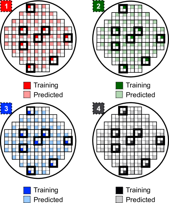
(b) Modeling and prediction using hierarchical GP regression

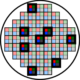
(c) All-site concatenation

Figure 3: Example of the site-based hierarchical GP regression, where a single touchdown has four sites.

Figure 3 depicts an example of the modeling using the proposed method when $S=4$ (sites 1 to 4). First, the eight positions are selected and measured as the training as shown in Fig. 3(a). In total, 32 dies ($=8\times 4$) are measured using the eight touchdowns. Then, according to the site, the GP-based modeling and prediction are individually applied, as in Fig. 3(b). In other words, for site 1, the measured value belonging to site 1 is used as training data to build a GP model, and the measured value of the unmeasured die belonging to site 1 is predicted. The measurements and predictions for the other sites are also similar. The entire prediction result is obtained through the concatenation as shown in Fig. 3(c).

III-B Active sampling under the multi-site testing

In the wafer-level spatial modeling, it is desirable to be given a small input training dataset to maximize the cost reduction of the measurement. In [10], an aggressive sampling method that preferentially measures the location with the largest predictive variance calculated by the GP regression is proposed. In addition, in [7], a Latin hypercube sampling approach [34] is employed to evenly choose random sample points over the entire wafer. However, these methods are straightforward, and most importantly, they do not consider multi-site testing environment.

A good model should be one with a small error between the model and the actual measurement. The mean squared error (MSE) against the test dataset can be expressed as:

$$E_{\rm MSE}=||{\bm{v}}||+||{\bm{\mu}}-{\bm{y}}_{\rm true}||^{2},$$ (8)

where $||\cdot||$ is the Euclidean norm, and ${\bm{y}}_{\rm true}$ is the correct value at the location of ${\bm{X}}_{\rm test}$ and unknown, i.e., unmeasured value. Assuming that the model is correct, the contribution of the second term in Eq. (8) to $E_{\rm MSE}$ is small compared to the variance contribution, that is, the first term. Thus, to minimize $E_{\rm MSE}$, we have to select ${\bm{X}}$ such that the overall variance of the estimator is minimized [25].

Algorithm 3 Active location selection with site-based hierarchical Gaussian process regression

1:${\bm{\mu}}$, ${\bm{v}}$ = hgpr$\left(({\bm{X}}_{\rm train},{\bm{y}}_{\rm train}),{\bm{X}}_{\rm test},f_{\rm kern}\right)$

2:for $p=1$ to $P$ do

3:     ${\bm{\mu}}_{p}$, ${\bm{v}}_{p}$ = hgpr(${\bm{X}}_{\rm train}+{\bm{X}}^{(p)}_{\rm add},{\bm{X}}_{\rm test},f_{\rm kern}$)

4:     Calculate the Euclidean distance between ${\bm{v}}$ and ${\bm{v}}_{p}$ as ${\Delta}^{(p)}_{{\rm var}}$

5:end for

6:Select ${\bm{X}}_{p}$ with the largest ${\Delta}^{(p)}_{{\rm var}}$ as the next touchdown location

Based on the aforementioned discussion, we propose an active sampling method as outlined in Algorithm 3, which is incorporated into the site-based hierarchical spatial modeling (hgpr) shown in Algorithm 2. The proposed sampling method focuses on the Euclidean distance between before and after measurements. The proposed method proceeds as follows. The numbers on the left indicate the corresponding line numbers in Algorithm 3.

• Calculate ${\bm{\mu}}$ and ${\bm{v}}$ through the hierarchical GP regression using $({\bm{X}}_{\rm train},{\bm{y}}_{\rm train})$ and ${\bm{X}}_{\rm test}$ as in Algorithm 2. ${\bm{X}}_{\rm train}$ can be obtained through multi-site testing.

• Repeat steps 3) and 4) for all touchdown location candidates. Here, the $p$-th touchdown candidate has ${\bm{X}}^{(p)}_{\rm test}=\{{\bm{x}}^{*(p)}_{1},{\bm{x}}^{*(p)}_{2},\cdots,{\bm{x}}^{*(p)}_{S}\}$ with the $S$ sites.

• Add the touchdown candidate ${\bm{X}}^{(p)}_{\rm add}$ by assuming it as measured and perform the hierarchical GP regression. Note that because it is not actually measured, we assume the mean values are measured as ${\bm{X}}^{(p)}_{\rm add}=\{({\bm{x}}^{*(p)}_{1},\mu^{(p)}_{1}),({\bm{x}}^{*(p)}_{2},\mu^{(p)}_{2}),\cdots,({\bm{x}}^{*(p)}_{S},\mu^{(p)}_{S})\}$, where $\mu^{(p)}_{S}$ is the predicted mean corresponding to ${\bm{x}}^{*(p)}_{S}$, and is one of the elements of ${\bm{\mu}}$ given by hgpr in step 1). In this step, ${\bm{\mu}}_{p}$ and ${\bm{v}}_{p}$ are obtained as in step 1).

• Calculate the Euclidean distance of ${\bm{v}}$ and ${\bm{v}}_{p}$ as ${\Delta}^{(p)}_{{\rm var}}$. Note that steps 2) to 5) are iterated for all the touchdown candidates.

• Select ${\bm{X}}_{p}$ with the largest ${\Delta}^{(p)}_{{\rm var}}$ as the next measurement location.

The mentioned procedure is iterated until an exit condition is satisfied, for example, a sufficient number of iterations are obtained. Because the reduction of the whole deviation for the test dataset is compared in step 6), a more accurate modeling can be expected with a smaller number of measurements compared to simply checking the location of the highest variance according to [25].

IV Numerical experiments

Figure 4: Heat map of fully measured characterization. The measured values are normalized.

Figure 5: Single touchdown with 16 sites in our multi-site testing.

IV-A Setup

To demonstrate the effectiveness of the proposed method, we conducted experiments using an industrial production test dataset of a 28 nm analog/RF device. Our dataset contains six lots. The first wafer of each lot was used for the evaluation; thus, we used six wafers with different lots. A single wafer has approximately 6,000 DUTs. In this experiment, we used a measured character for an item of the dynamic current test, in which site-to-site variability due to the multi-site test is noticeably observed, as shown in Figs. 1 and 2. A heat map of the full measurement results for the first wafer of the sixth lot is shown in Fig. 4. For the ease of experimentation, faulty dies were removed from the dataset. The number of sites in a single touchdown is 16, i.e., $S=16$. The form of a single touchdown is illustrated in Fig. 5. This is different from the rectangular touchdown illustrated in Fig. 3, which prevents interference on the probe of the impedance-matching circuits. As a result, a special pattern is observed during the multi-site test as shown in Fig. 4. To fully measure all DUTs on a single wafer, approximately 600 touchdowns are required.

All experiments were implemented in the Python language. The RBF kernel was used as the kernel function $f_{\rm kern}$ for the GP-based regression. The experiments were conducted on a Linux PC with an Intel Xeon Platinum 8160 2.10 GHz central processing unit using a single thread.

To quantitatively evaluate the modeling accuracy, we define the error ${\bm{\delta}}$ between the correct ${\bm{y}}_{\rm true}$ and the predicted mean ${\bm{\mu}}$ normalized by the maximum and minimum values of ${\bm{y}}_{\rm true}$ as follows:

$${\bm{\delta}}=\frac{{\bm{\mu}}-{\bm{y}}_{\rm true}}{d_{\rm spec}},$$ (9)

where $d_{\rm spec}$ is the range between the minimum and maximum values of the fully measured characteristics in Fig. 4.

IV-B Experimental results on site-based hierarchical spatial modeling

We first evaluated the site-based hierarchical spatial modeling presented in Algorithm 2. For comparison, naive GP regression-based approach (hereafter called naive GP) [9] and the two-step approach (hereafter called 2-step GP) [11] are also applied. Here, it should be noted that we do not consider the touchdown, that is, one-by-one measurement is conducted. The experimental result based on the touchdown is described later in Section IV-C.

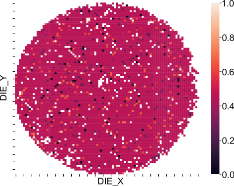
(a) Naive GP

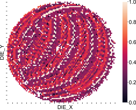
(b) 2-step GP

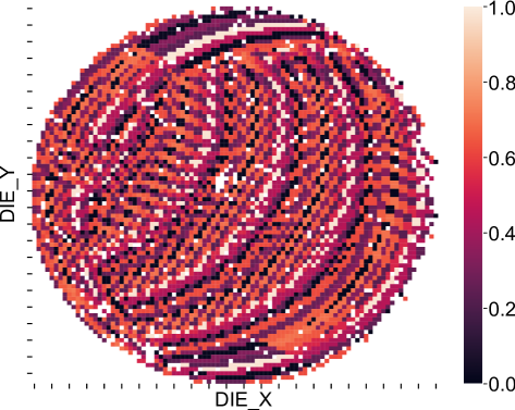
(c) Ours

Figure 6: Heat maps of the predicted characteristics by naive GP, 2-step GP, and the proposed method at the 10% spatial sampling rate. It can be visibly confirmed that the prediction results are closer to the actual measurements in the order of naive GP, 2-step GP, and the proposed method. The measured values are normalized.

For the 2-step GP method, the first wafer of the first lot is used to obtain $k$ clusters through $k$-means clustering. For the subsequent wafers, $k$ clusters were used to predict the device characteristics. In the experiment, the optimal $k$ was determined using the silhouette value and elbow method [31, 32] instead of Eq. (5), resulting in seven clusters.

In Fig. 6, the prediction results for the wafer of the sixth lot using each method are shown. They were predicted using randomly sampled values at a 10% spatial sampling rate. Clearly, the naive GP method fails to capture the site-to-site variation as shown in Fig. 6(a). In contrast, the specific pattern shown in Fig. 4 caused by the site-to-site variation can be confirmed in the 2-step GP method and our method as shown in Figs. 6(b) and 6(c). Figure 7 shows the box-plots of ${\bm{\delta}}$ using Eq. (9) for each method. In the figure, the top and bottom of the line represent the maximum and minimum values, respectively. The average is shown as a dot. The top and bottom of the box are 75% quantile and 25% quantile, respectively. The line represents the median. The average errors of ${\bm{\delta}}$ of the naive GP, 2-step GP method, and our method are 18.59%, 13.43%, and 0.69%, respectively. The proposed method can also drastically reduce the variance in the predictions. From the results, we can conclude that the proposed method can reduce the average error by approximately 5.13% compared to the 2-step GP method, i.e., $19.46$ times $(=13.43/0.69)$ more accurately.

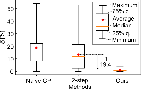
Figure 7: Box-plots of ${\bm{\delta}}$ for each method, where the maximum, 75% quantile, median, average, 25% quantile, and minimum values are shown.

Figure 8 shows the averages of ${\bm{\delta}}$ as a function of the spatial sampling rate using the three methods for the wafer of the sixth lot. Note that the prediction methods are not applied when the spatial sampling rate is 100% and the sampling rate is incrementally increased, that is, the measured locations at the 10% sampling rate are always contained at subsequent rates. As the spatial sampling rate increases, the averages of all the methods decrease monotonically. We also find that the average errors of the proposed method always achieves better prediction results for all the sampling rates.

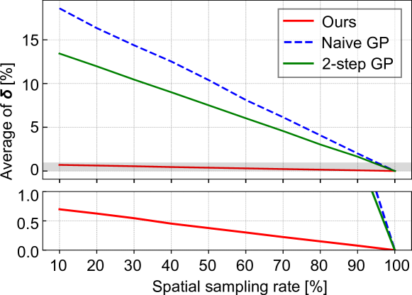
Figure 8: Averages of ${\bm{\delta}}$ obtained by naive GP, 2-step GP, and the proposed method at various sampling rates. The gray part is enlarged at the bottom of this figure.

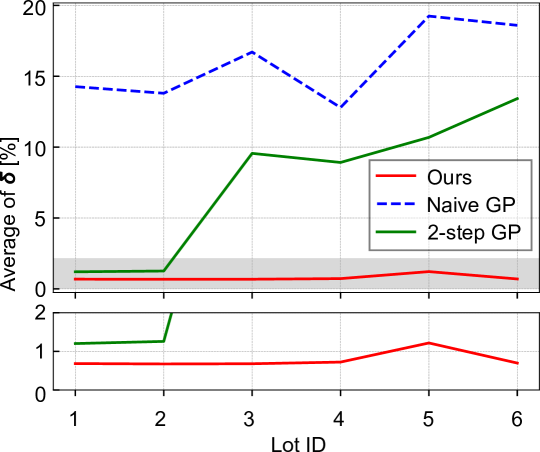
Figure 9: Changes of the averages of ${\bm{\delta}}$ for each lot. The gray part is enlarged at the bottom of this figure.

The averages of ${\bm{\delta}}$ for the wafer at the 10% sampling rate as a function of the lot ID are shown in Fig. 9. From the figure, it can be observed that the proposed method achieves the best estimation results for all the lots among the three methods. The prediction performance of the 2-step GP degrades as the production lot progresses, while the proposed method maintains a low prediction error below 2% regardless of the lot. This result implies that the $k$-means clustering result obtained in the first lot is inappropriate for subsequent lots.

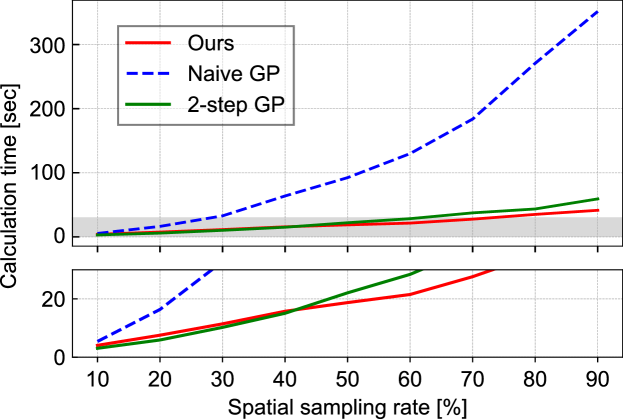
Figure 10: Calculation time. The gray part is enlarged at the bottom of this figure.

We evaluated the calculation time of the prediction for each method. Figure 10 summarizes the calculation time of each method for the sixth lot at various sampling rates. We can see that the proposed method and 2-step method can significantly reduce the calculation time compared to the naive GP method. This is due to the side benefits of hierarchical GP modeling approaches. In general, the inference time of GP is $\mathcal{O}(N^{3})$ scaled because of the computation of the matrix inverse [35, 36]. In the proposed method, GP modeling is conducted for each site individually, and thus the calculation time can be drastically reduced because the training samples are reduced to $N/S$ in each GP modeling, where $S$ is 16 for the proposed. The reduction becomes $N/k$ for the 2-step method, where $k=7$. Note that this calculation was conducted using a single thread. Therefore, the calculation time can be further reduced by implementing parallel processing.

IV-C Experimental result under multi-site testing

In the evaluation of the previous section, the sample dies are randomly selected one by one, and thus the multi-site test environment that measurements are conducted per site unit is not considered. We evaluated the sampling method listed in Algorithm 3 under the multi-site test environment. Here, it is assumed that the touchdown shown in Fig. 5 is performed in a single measurement. In all the existing researches of the wafer-level variation modeling, sampling is assumed one DUT at a time, and thus this work is the first to consider a multi-site testing environment for wafer-level variation modeling. In this experiment, the random sampling was used for comparison. First, we measured one randomly sampled touchdown and then selected the next one by the proposed method and random sampling.

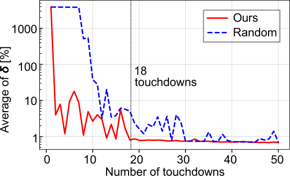
Figure 11: Averages of ${\bm{\delta}}$ as a function of the number of the touchdowns. The vertical axis is shown in log scale. The proposed method converges more quickly.

Figure 11 shows the average of ${\bm{\delta}}$ as a function of the number of the touchdowns that incrementally increased. The first wafer in the sixth lot was used. Though, an error of over 3000% is observed for both the methods at the first touchdown, the error is decreasing as increasing the number of the touchdowns for both methods. However, the random sampling method converges slowly, whereas the proposed method converges further quickly. More specifically, the proposed method has an average error of 0.80% or less with the 18 touchdowns, in contrast, the random sampling still has an average of 5.03%. The 18 touchdowns correspond to approximately 3% of the number of the touchdowns for full measurement. In addition, the random sampling does not converge even at the 50 touchdowns. It can be seen from the figure that the proposed sampling method can successfully reduce the number of the necessary touchdowns while achieving better prediction accuracy.

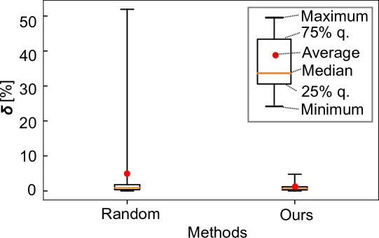
Figure 12: Box-plots of ${\bm{\delta}}$ for each method, where the maximum, 75% quantile, median, average, 25% quantile, and minimum values are shown. Because ${\bm{\delta}}$ of the random sampling is a multimodal distribution, the average is plotted out of the box.

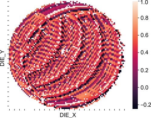
(a) Random sampling

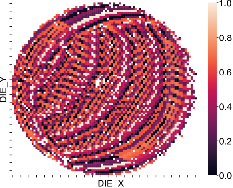
(b) Ours

Figure 13: Heat maps of the predicted characteristics for the 18 touchdowns.

The box-plots for the random sampling and the proposed method for the 18 touchdowns are shown in Fig. 12. It is clear that not only the average of ${\bm{\delta}}$ but also the variance of the estimation errors can be reduced by the proposed method. Although the random sampling has a maximum error of approximately 50%, the proposed method has only 4.77%. In Fig. 13, the prediction results for each method for the 18 touchdowns are shown. Although they are visually similar, in Fig. 13(a), the predicted values exceed the range of the normalized range, (i.e., 0 to 1), indicating that the predictions by the random sampling are not sufficient. On the other hand, excellent agreement is observed between Figs. 13(b) and 4. It shows that the proposed method successfully achieves highly accurate wafer-level variation modeling even in a multi-site test environment.

V Conclusion

In this paper, we proposed a novel wafer-level spatial correlation modeling method for multi-site RF IC testing. The proposed method employs GP regression, which is an efficient statistical modeling method used to predict the value for an unmeasured point from small sampling data. In the proposed method, GP is applied individually by partitioning the die location on a wafer according to the site information provided by the test engineers. In addition, we propose an active sampling method based on the predictive variance calculated by GP to achieve better prediction results while maintaining a small measurement cost. Experimental results using an industrial production test dataset demonstrated that the proposed method achieves a 19.46 times smaller prediction error than the conventional method. Moreover, we demonstrated that the proposed sampling method provides sufficient prediction accuracy with 18 touchdown measurements, which corresponds to 3% of the number of touchdowns for full measurement. In contrast, the prediction accuracy by random sampling required over 50 measurements. Although all the existing methods were evaluated with one DUT measurement, the proposed method achieved better prediction results by considering an actual touchdown under multi-site testing.

References

- [1] L.-C. Wang, “Experience of data analytics in EDA and test—principles, promises, and challenges,” IEEE Transactions on Computer-Aided Design of Integrated Circuits and Systems, vol. 36, no. 6, pp. 885–898, 2017.
- [2] H.-G. Stratigopoulos, “Machine learning applications in IC testing,” in Proceedings of IEEE European Test Symposium, 2018.
- [3] M. Shintani, M. Inoue, and Y. Nakamura, “Artificial neural network based test escape screening using generative model,” in Proceedings of IEEE International Test Conference, 2018, p. 9.2.
- [4] S. Reda and S. R. Nassif, “Accurate spatial estimation and decomposition techniques for variability characterization,” IEEE Transactions on Semiconductor Manufacturing, vol. 23, no. 3, pp. 345–357, 2010.
- [5] X. Li, R. R. Rutenbar, and R. D. Blanton, “Virtual probe: A statistically optimal framework for minimum-cost silicon characterization of nanoscale integrated circuits,” in Proceedings of IEEE/ACM International Conference on Computer-Aided Design, 2009, pp. 433–440.
- [6] W. Zhang, X. Li, and R. A. Rutenbar, “Bayesian virtual probe: Minimizing variation characterization cost for nanoscale IC technologies via Bayesian inference,” in Proceedings of ACM/EDAC/IEEE Design Automation Conference, 2010, pp. 262–267.
- [7] W. Zhang, X. Li, F. Liu, E. Acar, R. A. Rutenbar, and R. D. Blanton, “Virtual probe: A statistical framework for low-cost silicon characterization of nanoscale integrated circuits,” IEEE Transactions on Computer-Aided Design of Integrated Circuits and Systems, vol. 30, no. 7, pp. 1814–1827, 2011.
- [8] S. Zhang, F. Lin, C.-K. Hsu, K.-T. Cheng, and H. Wang, “Joint virtual probe: Joint exploration of multiple test items’ spatial patterns for efficient silicon characterization and test prediction,” in Proceedings of IEEE Design Automation and Test in Europe, 2014.
- [9] N. Kupp, K. Huang, J. M. Carulli, Jr., and Y. Makris, “Spatial correlation modeling for probe test cost reduction in RF devices,” in Proceedings of IEEE/ACM International Conference on Computer-Aided Design, 2012, pp. 23–29.
- [10] A. Ahmadi, K. Huang, S. Natarajan, C. John M., Jr., and Y. Makris, “Spatio-temporal wafer-level correlation modeling with progressive sampling: A pathway to HVM yield estimation,” in Proceedings of IEEE International Test Conference, 2014, p. 18.1.
- [11] K. Huang, N. Kupp, C. John M., Jr., and Y. Makris, “Handling discontinuous effects in modeling spatial correlation of wafer-level analog/RF tests,” in Proceedings of IEEE Design Automation and Test in Europe, 2013, pp. 553–558.
- [12] E. J. Marinissen, A. Singh, D. Glotter, M. Esposito, J. M. C. Jr., A. Nahar, K. M. Butler, D. Appello, and C. Portelli, “Adapting to adaptive testing,” in Proceedings of IEEE Design Automation and Test in Europe, 2010, pp. 556–561.
- [13] K. R. Gotkhindikar, W. R. Daasch, K. M. Butler, J. M. Carulli, Jr., and A. Nahar, “Die-level adaptive test: Real-time test reordering and elimination,” in Proceedings of IEEE International Test Conference, 2011, p. 15.1.
- [14] E. Yilmaz, S. Ozev, O. Sinanoglu, and P. Maxwell, “Adaptive testing: Conquering process variations,” in Proceedings of IEEE European Test Symposium, 2012.
- [15] M. Shintani, T. Uezono, T. Takahashi, K. Hatayama, T. Aikyo, K. Masu, and T. Sato, “A variability-aware adaptive test flow for test quality improvement,” IEEE Transactions on Computer-Aided Design of Integrated Circuits and Systems, vol. 33, no. 7, pp. 1056–1066, 2014.
- [16] A. P. Dempster, N. M. Laird, and D. B. Rubin, “Maximum likelihood from incomplete data via the EM algorithm,” Journal of the Royal Statistical Society. Series B (Methodological), vol. 39, no. 1, pp. 1–38, 1977.
- [17] D. L. Donoho, “Compressed sensing,” IEEE Transactions on Information Theory, vol. 52, no. 4, pp. 1289–1306, 2006.
- [18] E. J. Candes and M. B. Wakin, “An introduction to compressive sampling,” IEEE Signal Processing Magazine, vol. 25, no. 2, pp. 21–30, 2008.
- [19] C. E. Rasmussen and C. K. I. Williams, Gaussian Processes for Machine Learning. MIT Press, 2006.
- [20] N. Sumikawa, L.-C. Wang, and M. S. Abadir, “An experiment of burn-in time reduction based on parametric test analysis,” in Proceedings of IEEE International Test Conference, 2012, p. 19.3.
- [21] T. Lehner, A. Kuhr, M. Wahl, and R. Brück, “Site dependencies in a multisite testing environment,” in Proceedings of IEEE European Test Symposium, 2014.
- [22] P. O. Farayola, S. K. Chaganti, A. O. Obaidi, A. Sheikh, S. Ravi, and D. Chen, “Quantile – quantile fitting approach to detect site to site variations in massive multi-site testing,” in Proceedings of IEEE VLSI Test Symposium, 2020.
- [23] D. Steinley, “K-means clustering: A half-century synthesis,” British Journal of Mathematical and Statistical Psychology, vol. 59, no. 1, pp. 1–34, 2006.
- [24] K. M. Butler, A. Nahar, and W. R. Daasch, “What we know after twelve years developing and deploying test data analytics solutions,” in Proceedings of IEEE International Test Conference, 2016.
- [25] S. Seo, M. Wallat, T. Graepel, and K. Obermayer, “Gaussian process regression: active data selection and test point rejection,” in Proceedings of IEEE-INNS-ENNS International Joint Conference on Neural Networks, 2000, pp. 241–246.
- [26] C. M. Bishop, Pattern Recognition and Machine Learning. Springer, 2006.
- [27] D. Duvenaud, “The kernel cookbook,” [Online]. Available: https://www.cs.toronto.edu/ duvenaud/cookbook/.
- [28] M. G. Genton, “Classes of kernels for machine learning: A statistics perspective,” The Journal of Machine Learning Research, vol. 2, pp. 299–312, 2001.
- [29] S. Ohkawa, M. Aoki, and H. Masuda, “Analysis and characterization of device variations in an LSI chip using an integrated device matrix array,” IEEE Transactions on Semiconductor Manufacturing, vol. 17, no. 2, pp. 155–165, 2004.
- [30] S. Saxena, C. Hess, H. Karbasi, A. Rossoni, S. Tonello, P. McNamara, S. Lucherini, S. Minehane, C. Dolainsky, and M. Quarantelli, “Variation in transistor performance and leakage in nanometer-scale technologies,” IEEE Transactions on Electron Devices, vol. 55, no. 1, pp. pp131–pp144, 2008.
- [31] P. J. Rousseeuw, “Silhouettes: A graphical aid to the interpretation and validation of cluster analysis,” in Journal of Computational & Applied Mathematics, 1987, pp. 53–65.
- [32] C. Goutte, P. Toft, E. Rostrup, F. A. Nielsen, and L. K. Hansen, “On clustering fMRI time series,” NeuroImage, vol. 9, pp. 298–310, 1999.
- [33] T. Calinski and J. Harabasz, “A dendrite method for cluster analysis,” Communications in Statistics, vol. 3, pp. 1–27, 1974.
- [34] B. Tang, “Orthogonal array-based latin hypercubes,” Journal of the American Statistical Association, vol. 88, no. 424, pp. 1392–1397, 1991.
- [35] S. Park and S. Choi, “Hierarchical Gaussian process regression,” in Proceedings of Asian Conference on Machine Learning, 2010, pp. 95–110.
- [36] D.-T. Nguyen, M. Filippone, and P. Michiardi, “Exact Gaussian process regression with distributed computations,” in Proceedings of ACM/SIGAPP Symposium on Applied Computing, 2019, pp. 1286–1295.