Koopman Q-learning: Offline Reinforcement Learning
via Symmetries of Dynamics

Abstract

Offline reinforcement learning leverages large datasets to train policies without interactions with the environment. The learned policies may then be deployed in real-world settings where interactions are costly or dangerous. Current algorithms over-fit to the training dataset and as a consequence perform poorly when deployed to out-of-distribution generalizations of the environment. We aim to address these limitations by learning a Koopman latent representation which allows us to infer symmetries of the system’s underlying dynamic. The latter is then utilized to extend the otherwise static offline dataset during training; this constitutes a novel data augmentation framework which reflects the system’s dynamic and is thus to be interpreted as an exploration of the environment’s state space. To obtain the symmetries we employ Koopman theory in which non-linear dynamics are represented in terms of a linear operator acting on the space of measurement functions of the system. We provide novel theoretical results on the existence and nature of symmetries relevant for control systems such as reinforcement learning settings. Moreover, we empirically evaluate our method on several benchmark offline reinforcement learning tasks and datasets including D4RL, Metaworld and Robosuite and find that by using our framework we consistently improve the state-of-the-art of model-free Q-learning methods.

1 Introduction

The recent impressive advances in reinforcement learning (RL) range from robotics, to strategy games and recommendation systems (Kalashnikov et al., 2018; Li et al., 2010). Reinforcement learning is canonically regarded as an active learning process - also referred to as online RL - where the agent interacts with the environment at each training run. In contrast, offline RL algorithms learn from large, previously collected static datasets, and thus do not rely on environment interactions (Agarwal et al., 2020; Ernst et al., 2005; Fujimoto et al., 2019). Online data collection is performed by simulations or by means of real world interactions e.g. robotics and in either scenario interactions maybe costly and/or dangerous.

In principle offline datasets only need to be collected once which alleviates the before-mentioned shortcomings of costly online interactions. Offline datasets are typically collected using behavioral policies for the specific task ranging from, random policies, or near-optimal policies to human demonstrations. In particular, being able to leverage the latter is a major advantage of offline RL over online approaches, and then the learned policies can be deployed or fine-tuned on the desired environment. Offline RL has successfully been applied to learn agents that outperform the behavioral policy used to collect the data (Kumar et al., 2020; Wu et al., 2019; Agarwal et al., 2020; Ernst et al., 2005). However algorithms admit major shortcomings in regard to over-fitting and overestimating the true state-action values of the distribution. One solution was recently proposed by Sinha et al. (2021), where they tested several data augmentation schemes to improve the performance and generalization capabilities of the learned policies.

However, despite the recent progress, learning from offline demonstrations is a tedious endeavour as the dataset typically does not cover the full state-action space. Moreover, offline RL algorithms per definition do not admit the possibility for further environment exploration to refine their distributions towards an optimal policy. It was argued previously that is basically impossible for an offline RL agent to learn an optimal policy as the generalization to near data generically leads to compounding errors such as overestimation bias (Kumar et al., 2020). In this paper, we look at offline RL through the lens of Koopman spectral theory in which non-linear dynamics are represented in terms of a linear operator acting on the space of measurement functions of the system. Through which the representation the symmetries of the dynamics may be inferred directly, and can then be used to guide data augmentation strategies see Figure 1. We further provide theoretical results on the existence on nature of symmetries relevant for control systems such as reinforcement learning. More specifically, we apply Koopman spectral theory by: first learning symmetries of the system’s underlying dynamic in a self-supervised fashion from the static dataset, and second employing the latter to extend the offline dataset at training time by out-of-distribution values. As this reflects the system’s dynamics the additional data is to be interpreted as an exploration of the environment’s state space.

Some prior works have explored symmetry of the state-action space in the context of Markov Decision Processes (MDP’s) (Higgins et al., 2018; Balaraman & Andrew, 2004; van der Pol et al., 2020) since many control tasks exhibit apparent symmetries e.g. the cart-pole is translation symmetric w.r.t. its position. The paradigm introduced in this work is of a different nature entirely. The distinction is twofold: first, the symmetries are learned in a self-supervised way and are in general not apparent to the developer; second: we concern with symmetry transformation from state tuples $(s_{t},s_{t+1})\to(\tilde{s}_{t},\tilde{s}_{t+1})$ which leave the action invariant. The latter, are inferred from the dynamics inherited by the behavioral policy of the underlying offline data. In other words we seek to derive a neighbourhood around a MDP tuple in the offline dataset in which the behavioral policy is likely to choose the same action based on its dynamics in the environment. In practice the Koopman latent space representation is learned in a self-supervised manner by training to predict the next state using a VAE model (Kingma & Welling, 2013).

To summarize, in this paper, we propose Koopman Forward (Conservative) Q-learning (KFC): a model-free Q-learning algorithm which uses the symmetries in the dynamics of the environment to guide data augmentation strategies. We also provide thorough theoretical justifications for KFC. Finally, we empirically test our approach on several challenging benchmark datasets from D4RL (Fu et al., 2021), MetaWorld (Yu et al., 2019) and Robosuite (Zhu et al., 2020) and find that by using KFC we can improve the state-of-the-art on most benchmark offline reinforcement learning tasks.

2 Preliminaries and background

2.1 Offline RL & Conservative Q-learning

Reinforcement learning algorithms train policies to maximize the cumulative reward received by an agent who interacts with an environment. Formally the setting is given by a Markov decision process $(\mathcal{S},\mathcal{A},\rho,r,\gamma)$, with state space $\mathcal{S}$, action space $\mathcal{A}$, and $\rho(s_{t+1}|s_{t},a_{t})$ the transition density function from the current state and action to the next state. Moreover, $\gamma$ is the discount factor and $r(S_{t})$ the reward function. At any discrete time the agent chooses an action $a_{t}\in\mathcal{A}$ according to its underlying policy $\pi_{\theta}(a_{t}|s_{t})$ based on the information of the current state $s_{t}\in\mathcal{S}$ where the policy is parametrized by $\theta$.

We focus on the Actor-Critic methods for continuous control tasks in the following. In deep RL the parameters $\theta$ are the weights in a deep neural network function approximation of the policy or Actor as well as the state-action value function $Q$ or Critic, respectively, and are optimized by gradient decent. The agent i.e. the Actor-Critic is trained to maximize the expected $\gamma$-discounted cumulative reward $\mathbb{E}_{\pi}[\sum_{t=0}^{T}\gamma^{t}\,r_{\pi}(s_{t},a_{t})]$, with respect to the policy network i.e. its parameters $\theta$. For notational simplicity we omit the explicit dependency of the latter in the remainder of this work. Furthermore the state-action value function $Q(s_{t},a_{t})$, returns the value of performing a given action $a_{t}$ while being in the state $s_{t}$. The Q-function is trained by minimizing the Bellman error as

$$\hat{Q}_{i+1}\leftarrow\arg\min_{Q}\mathbb{E}\Big{[}\big{(}r_{t}+\gamma\,\hat{Q}_{i}(s_{t+1},a_{t+1})-Q(s_{t},a_{t})\big{)}^{2}\Big{]}\,.$$ (1)

This is commonly referred to as the i${}^{\text{th}}$ policy evaluation step where the hat denotes the target Q-function. In offline RL one aims to learn an optimal policy for the given the dataset $\mathcal{D}=\bigcup_{k=1,\dots,\text{\#data-points}}\big{(}s_{t},a_{t},r_{t},s_{t+1}\big{)}_{k}$ as the option for exploration of the MDP is not available. The policy is optimized to maximize the state-action value function via the policy improvement

$$\pi_{i+1}\leftarrow\arg\max_{\pi}\mathbb{E}_{s_{t}\sim\mathcal{D}}\big{[}\hat{Q}_{i}\big{(}s_{t},\pi(a_{t}|s_{t})\big{)}\big{]}\;.$$ (2)

CQL algorithm: CQL is built on top of a Soft Actor-Critic algorithm (SAC) (Haarnoja et al., 2018), which employs soft-policy iteration of a stochastic policy (Haarnoja et al., 2017). A policy entropy regularization term is added to the policy improvement step in Eq. (2) as

$$\pi_{i+1}\leftarrow\arg\max_{\pi}\underset{s_{t}\sim\mathcal{D}}{\mathbb{E}}\Big{[}\hat{Q}_{i}\big{(}s_{t},\pi(a_{t}|s_{t})\big{)}-\alpha\log\pi(a_{t}|s_{t})\Big{]}\,$$ (3)

where $\alpha$ either is a fixed hyperparameter or may be chosen to be trainable.

CQL reduces the overestimation of state-values - in particular those out-of distribution from $\mathcal{D}$. It achieves this by regularizing the Q-function in Eq. (1) by a term minimizing its values over out of distribution randomly sampled actions. In the following $a_{t+1}$ is given by the prediction of the policy $\pi_{i}(a_{t+1}|s_{t+1})$. The policy optimisation step Eq. (1) is modified by a regulizer term

$$\arg\min_{Q}\underset{s_{t}\sim\mathcal{D}}{\mathbb{E}}\Big{[}\log\sum_{a}\exp\big{(}Q(s_{t},a)\big{)}-\underset{a\sim\pi(s_{t})}{\mathbb{E}}\big{[}Q(s_{t},a)\big{]}\Big{]}\ .$$ (4)

Where we have omitted the hyperparameter $\tilde{\alpha}$ balancing the regulizer term in Eq. (4).

Figure 1: Overview of Koopman Q-learning. The states of the data point $(s_{t},s_{t+1},a_{t})$ are shifted along symmetry trajectories parametrized by $\epsilon_{1,2,3}$ for constant $a_{t}$. Symmetry transformations can be combined to reach other specific subset of the $\epsilon$-ball region.

2.2 Koopman theory

Historically, the Koopman theoretic perspective of dynamical systems was introduced to describe the evolution of measurements of Hamiltonian systems (Koopman, 1931; Mezić, 2005). The underlying dynamic of most modern reinforcement learning tasks is of non-linear nature, i.e. the agents actions lead to changes of it state described by a complex non-linear dynamical system. In contrast to linear systems which are completely characterized by their spectral decomposition non-linear systems lack such a unified characterisation.

The Koopman operator theoretic framework describes non-linear dynamics via a linear infinite-dimensional Koopman operator and thus inherits certain tools applicable to linear control systems (Mauroy et al., 2020; Kaiser et al., 2021). In practice one aims to find a finite-dimensional representation of the Koopman operator which is equivalent to obtaining a coordinate transformations in which the non-linear dynamics are approximately linear. A general non-affine control system is governed by the system of non-linear ordinary differential equations (ODEs) as

$$\dot{s}=f(s,a)\;\;,$$ (5)

where $s,$ is the n-dimensional state vector, $a$ the m-dimensional action vector with $(s,a)\in\mathcal{S}\times\mathcal{A}$ the state-action-space. Moreover, $\dot{s}=\partial_{t}s$ is the time derivative, and $f$ is some general non-linear - at least $\mathcal{C}^{1}$-differentiable - vector valued function. For a discrete time system, Eq. (5) takes the form

$$s_{t+1}=F(s_{t},a_{t})\;\;,$$ (6)

where $s_{t}$ denotes the state at time $t$ where F is at least $\mathcal{C}^{1}$-differentiable vector valued function.

Definition 2.1 (Koopman operator).

Let $\mathscr{K}(\mathcal{S}\times\mathcal{A})$ be the (Banach) space of all measurement functions (observables). Then the Koopman operator $\mathcal{K}:\mathscr{K}(\mathcal{S}\times\mathcal{A})\to\mathscr{K}(\mathcal{S}\times\mathcal{A})$ is defined by

$$\mathcal{K}g(s_{t},a_{t})=g\big{(}F(s_{t},a_{t}),a_{t+1}\big{)}=g(s_{t+1},a_{t+1})\;,\;\;$$ (7)

for all observables $g\in\mathscr{K}(\mathcal{S}\times\mathcal{A})$ where $g:\mathcal{S}\times\mathcal{A}\to\mathbb{R}$.

Many systems can be modeled by a bilinearisation where the action enters the controlling equations 5 linearly as

$$f(s,a)=f_{0}(s)+\sum_{i}^{m}f_{i}(s)a_{i}\;\;,$$ (8)

for $f_{i},\,i=0,\dots,m$  $\mathcal{C}^{1}$-differentiable-vector valued functions. In that case the action of the Koopman operator takes the simple form

$$g(s_{t+1})=\mathcal{K}(a)g(s_{t})=\Big{(}\mathcal{K}_{0}+\sum_{i}^{m}\mathcal{K}_{i}a_{i}\Big{)}g(s_{t})\;,\vspace{-0.1cm}$$ (9)

$\forall g\in\mathscr{K}(\mathcal{S})$ where $\mathscr{K}(\mathcal{S})$ is a (Banach) space of measurement functions $\mathcal{K}_{0},\mathcal{K}_{i}$ decompose the Koopman operator in a the free and forcing-term, respectively. Details on the existence of a representation as in Eq. (9) are discussed in (Goswami & Paley, 2017). Associated with a Koopman operator is its eigenspectrum, that is, the eigenvalues $\lambda$, and the corresponding eigenfunctions $\varphi_{\lambda}(s,a)$, such that

$$\mathcal{K}\varphi_{\lambda}(s,a)=\lambda\varphi_{\lambda}(s,a)\;\;.$$ (10)

In practice one derives a finite set of observable

$$\vec{g}=(g_{1},\dots,g_{N})\;\;,$$

in which case the approximation to the Koopman operator admits a finite-dimensional matrix representation. The $N\times N$ matrix representing the Koopman operator may be diagonalized by a matrix $U$ containing the eigen-vectors of $\mathcal{K}$ as columns. In which case the eigen-functions are derived by $\vec{\varphi}=U\vec{g}$ and one infers from Eq. (5) that $\dot{\varphi}_{i}=\lambda_{i}\varphi_{i}\;,\;\;\text{for}\;\;i=1,\dots,N$ with eigenvalues $\lambda_{i=1,\dots,N}$. These ODEs admit simple solutions for their time-evolution namely the exponential functions $\exp(\lambda_{i}t)$.

3 The Koopman forward framework

We initiate our discussion with a focus on symmetries in dynamical control systems in Subsection 3.1 where we additionally present some theoretical results. We then proceed in Subsection 3.2 by presenting the Koopman forward framework for Q-learning based on CQL. Moreover, we discuss the algorithm as well as the Koopman Forward model’s deep neural network architecture.

3.1 Symmetries of dynamical control systems

Informal Overview: Our theoretical results culminate in theorem 3.8 and 3.9, which provides a road-map on how specific symmetries of the dynamical control system are to be inferred from a VAE forward prediction model. In particular, theorem 3.8 guarantees that the procedure leads to symmetries of the system (at least locally) and theorem 3.9 that actual new data points can be derived by applying symmetry transformations to existing ones. To make this topic more approachable we have shifted some technical details to the appendix A.

For the reader who wants to skip this technical section directly to the algorithm in section 3.2 let us summarize a couple of take-away messages. Trajectories of many RL-environments are often solutions of ODEs. Symmetries can map solutions i.e. trajectories to each other. Thus having solutions (offline RL data) the symmetry map provides one the tools to generate novel data points. However, symmetry maps are hard to come by. In this section we provide a principled approach on how to derive this symmetry maps for control system using Koopman theory. Vaguely an operator is a symmetry generator if it commutes with the Koopman operator.

In general, a symmetry group $\Sigma$ of the state space may be any subgroup of the group of isometrics of the Euclidean space. We consider Euclidean state spaces and in particular, $\Sigma$ invariant compact subsets thereof.

Definition 3.1 (Equivariant Dynamical System).

Consider the dynamical system $\dot{s}=f(s)$ and let $\Sigma$ be a group acting on the state-space $\mathcal{S}$. Then the system is called $\Sigma$-equivariant if $f(\sigma\cdot s)=\sigma\cdot f(s)\;,\;\;\text{for}\;s\in\mathcal{S}\;,\;\;\forall\sigma\in\Sigma$. For a discrete time dynamical system $s_{t+1}=F(s_{t})$ one defines equivariance analogously, namely if $F(\sigma\cdot s_{t})=\sigma\cdot F(s_{t})$ , for $\;s_{t}\in\mathcal{S}\;,\;\;\forall\sigma\in\Sigma$.

A system of ODEs may be represented by the set of its solutions which are locally connected by Lie Groups. In other words the symmetry maps are given by elements of the Lie Group which map between solutions.

Definition 3.2 (Symmetries of ODEs).

A symmetry of a system of ODEs on a locally-smooth structure is a locally-defined diffeomorphism that maps the set of all solutions to itself.

Definition 3.3 (Local Lie Group).

A parametrized set of transformations $\sigma^{\epsilon}:\mathcal{S}\to\mathcal{S}$ with $s\mapsto\tilde{s}(s,\epsilon)$ for $\epsilon\in(\epsilon_{low},\epsilon_{high})$ where $\epsilon_{low}<0<\epsilon_{high}$ is a one-parameter local Lie group if

1. $\sigma^{0}$ is the identity map; for $\epsilon=0$ such that $\tilde{s}(s,0)=s$.

2. $\sigma^{\epsilon_{1}}\sigma^{\epsilon_{2}}=\sigma^{\epsilon_{2}}\sigma^{\epsilon_{1}}=\sigma^{\epsilon_{1}+\epsilon_{2}}$ for every $|\epsilon_{1}|,|\epsilon_{2}|\ll 1$.

3. $\tilde{s}(s,\epsilon)$ admits a Taylor series expansion in $\epsilon$; in a neighbourhood of $s$ determined by $\epsilon=0$ as $\tilde{s}(s,\epsilon)=s+\epsilon\,\zeta(s)+\mathcal{O}(\epsilon^{2})$.

The Koopman operator of equivariant dynamical system is reviewed in the appendix A. Let us next turn to the case relevant for RL, namely control systems. In the remainder of this section we focus on dynamical systems given as in Eq. (6) and Eq. (9).

Definition 3.4 (Action-Equivariant Dynamical System).

Let $\bar{\Sigma}$ be a group acting on the state-action-space $\mathcal{S}\times\mathcal{A}$ of a general control system as in Eq. (6) such that it acts as the identity operation on $\mathcal{A}$ i.e. $\sigma\cdot(s_{t},a_{t})=(\sigma|_{\mathcal{S}}\cdot s_{t},a_{t})\;,\;\;\forall\sigma\in\bar{\Sigma}\;\;.$ Then the system is called $\bar{\Sigma}$-action-equivariant if

$$F(\sigma\cdot(s_{t},a_{t}))=\sigma|_{\mathcal{S}}\cdot F(s_{t},a_{t})\;,\;\;\text{for}\;(s_{t},a_{t})\in\mathcal{S}\times\mathcal{A}\;.$$ (11)

Lemma 3.5.

The map $\bar{\ast}:\bar{\Sigma}\times\mathscr{K}(\mathcal{S}\times\mathcal{A})\rightarrow\mathscr{K}(\mathcal{S}\times\mathcal{A})$ given by $(\sigma\bar{\ast}g)(s,a)\longmapsto g(\sigma^{-1}\cdot s,a)$ defines a group action on the Koopman space of observables $\mathscr{K}(\mathcal{S}\times\mathcal{A})$.

Theorem 3.6.

A Koopman operator $\mathcal{K}$ of a $\bar{\Sigma}$-action-equivariant system $s_{t+1}=F(s_{t},a_{t})$ satisfies

$$[\sigma\bar{\ast}(\mathcal{K}g)](s_{t},a_{t})=[\mathcal{K}(\sigma\bar{\ast}g)](s_{t},a_{t})\;\;.$$ (12)

In particular, it is easy to see that the biliniarisation in Eq. (9) is $\Sigma$-action-equivariant if $f_{i}(\sigma|_{\mathcal{S}}\cdot s)=\sigma|_{\mathcal{S}}\cdot f_{i}(s)\;,\;\;\forall i=0,\dots,m$. Let us thus turn our focus on the relevant case of a control system $s_{t+1}=\tilde{F}(s_{t},a_{t})$ which admits a Koopman operator description as

$$g(s_{t+1})=\mathcal{K}(a_{t})g(s_{t})\;,\;\;\text{for}\;a_{t}\in\mathcal{A}\,,\;\forall g\in\mathscr{K}(\mathcal{S})\;\;,$$ (13)

where $\{\mathcal{K}(a)\}_{a\in\mathcal{A}}$ is a family of operators with analytical dependence on $a\in\mathcal{A}$. Note that the bilinearisation in Eq. (9) is a special case of Eq. (13).

Definition 3.7 ($\hat{\Sigma}$-Action-Equivariant Control System ).

We refer to a control system as in Eq. (13) admitting a symmetry map $\hat{\ast}$ as $\hat{\Sigma}$-action-equivariant. The definition of the map $\hat{\ast}$ is a bit more involved, see the appendix A.9. Informally, we note that it will connect a symmetry map depending on the action space $\sigma_{a}$ and the Koopman observable as $(\sigma_{a}\hat{\ast}g)(s)\longmapsto g(\sigma^{-1}\cdot s)$. The latter, defines a group action on the Koopman space of observables $\mathscr{K}(\mathcal{S})$.

Theorem 3.8.

Let $s_{t+1}=\tilde{F}(s_{t},a_{t})$ be a $\hat{\Sigma}$-action-equivariant control system i.e. admitting a symmetry action as in definition 3.7 and a Koopman operator representation as

$$g(s_{t+1})=\mathcal{K}(a_{t})g(s_{t})\;,\;\;\text{for}\;a_{t}\in\mathcal{A}\,,\;\forall g\in\mathscr{K}(\mathcal{S})\;\;.$$ (14)

Then

$$\big{[}\sigma_{a_{t}}\hat{\ast}\big{(}\mathcal{K}(a_{t})g\big{)}\big{]}(s_{t})=\big{[}\mathcal{K}(a_{t})\,\big{(}\sigma_{a_{t}}\hat{\ast}g\big{)}\big{]}(s_{t})\;\;.$$ (15)

Moreover, a control system obeying equations 14 and 15 is $\hat{\Sigma}$-action-equivariant locally if $g^{-1}$ exists for a neighborhood of $s_{t}$, i.e. then $\sigma\cdot\tilde{F}(s_{t},a_{t})=\tilde{F}(\sigma\cdot(s_{t},a_{t}))$.

To allow an easier transition to the empirical section we introduce the notation $E:\mathcal{S}\to\mathscr{K}(S)$ and $D:\mathscr{K}(S)\to\mathcal{S}$, denoting the $\mathcal{C}^{1}$-differentiable encoder and decoder to and from the finite-dimensional Koopman space approximation, respectively;  $E\circ D=D\circ E=id$. Data-points may be shifted by symmetry transformations of solutions of ODEs as discussed next.

Theorem 3.9.

Let $s_{t+1}=\tilde{F}(s_{t},a_{t})$ be a control system as in Eq. (14) and $\sigma_{a_{t}}$ an operator obeying Eq. (15). Then $\sigma_{a_{t}}^{\epsilon}:\big{(}s_{t},s_{t+1},a_{t}\big{)}\longmapsto\big{(}\tilde{s}_{t},\tilde{s}_{t+1},a_{t}\big{)}$ with

$$\tilde{s}_{t} = D\Big{(}\,\big{(}\mathds{1}\;+\;\epsilon\,\sigma_{a_{t}}\big{)}\hat{\ast}E(s_{t})\Big{)}\;,$$ (16)

$$\tilde{s}_{t+1} = D\Big{(}\,\big{(}\mathds{1}\;+\;\epsilon\,\sigma_{a_{t}}\big{)}\hat{\ast}E(s_{t+1})\Big{)}\;\;\,$$

is a one-parameter local Lie symmetry group of ODEs. In other words one can use a symmetry transformation to shift both $s_{t}$ as well as $s_{t+1}$ such that $\tilde{s}_{t+1}=\tilde{F}(\tilde{s}_{t},a_{t})$.

3.2 KFC algorithm

The previous section provides a theoretical foundation to derive symmetries of dynamical control systems based on a Koopman latent space representation. A vague take-away message is that an operator is a symmetry generator if it commutes with the Koopman operator. Thus the algorithmic challenge of our framework is twofold. Firstly, to find a numerical approximation of the Koopman space and Koopman operator and secondly to derive operators which commute with the latter.

In practice the Koopman latent space representation is finite-dimensional a so called Koopman invariant subspace. As a consequence the Koopman operator and the symmetry generators admit finite matrix representations. To derive the Koopman representation there exist elaborate techniques such as e.g. (Morton et al., 2019) which have shown significant advantages over a basic variational auto-encoder (VAE). However, we use the latter for simplicity. Lastly, after having learned a Koopman representation and derived symmetry maps the objective is to generate augmented data points; which are then used by the Q-learning algorithm such as CQL at training-time.

The KFC-algorithm :

• Step 1: Train the Koopman forward model to learn the Koopman latent representation.

• Step 2: Compute the symmetry transformations $\sigma_{a}^{\epsilon}$; we use two approaches denoted by KFC and KFC++.

• Step 3: Integration into Q-learning algorithm; replace input data $(s_{t},s_{t+1},a,r)\mapsto(\sigma_{a}^{\epsilon}(s_{t}),\sigma_{a}^{\epsilon}(s_{t+1}),a,r)$ .

Step 1: Pre-training of a Koopman forward model

$$\mathcal{F}^{c}(s_{t},a_{t})=\begin{cases}{\bf c=0\;\;\text{VAE}:}\;\;D\big{(}E(s_{t})\big{)}=s_{t}\vspace{0,25 cm}\\ {\bf c=1\;\;\text{forward prediction}:}\vspace{0,1 cm}\\ D\Big{(}\,\big{(}\mathcal{K}_{0}+\sum_{i=1}^{m}\mathcal{K}_{i}\,a_{t,i}\big{)}E(s_{t})\,\Big{)}=s_{t+1}\end{cases}\vspace{0,1 cm}\,.$$ (17)

Both $E$ and $D$ are approximated by Multi-Layer-Perceptrons (MLPs) and the bilinear Koopman-space operator is implemented as fully connected layers (no bias) with weight matrices $\mathcal{K}_{i},\,i=0,\dots,m$, respectively. For training details we refer the reader to Appendix C.

Step 2: Computation of symmetry transformations

From theorem 3.9 one infers that in order for Eq. (3.2) to be a local Lie symmetry group of the approximate ODEs captured by the neural net Eq. (17) one needs $\sigma_{a_{t}}$ to commute with the approximate Koopman operator in Eq. (17).

For the KFC option in Eq. (3.2) the symmetry generator matrix $\sigma_{a}$ is obtained by solving the equation

$$\sigma_{a_{t}}\cdot\mathcal{K}(a_{t})-\mathcal{K}(a_{t})\cdot\sigma_{a_{t}}=0\;\;,$$

which may be accomplished by employing a Sylvester algorithm (syl, ). For KFC++ we compute the eigen-vectors of $\mathcal{K}(a_{t})$ which then constitute the columns of $U(a_{t})$. Thus in particular one infers that

$$\big{[}\;\sigma_{a_{t}}(\vec{\epsilon})\,,\,\mathcal{K}(a_{t})\;\big{]}=0\;\;,$$

The latter, is solved by construction of $\sigma_{a_{t}}(\vec{\epsilon})$ which commutes with the Koopman operator for all values of the random variables. The symmetry shifts in latent space are given by

KFC: $$\;\;{\bf\sigma^{\epsilon}_{a_{t}}:}\,s\mapsto\tilde{s}=D\Big{(}\big{(}\mathds{1}+\epsilon\sigma_{a_{t}}\big{)}E(s)\Big{)}$$

KFC++: $$\;\;{\bf\sigma^{\epsilon}_{a_{t}}:}\,s\mapsto\tilde{s}=D\Big{(}\big{(}\mathds{1}+\sigma_{a_{t}}(\vec{\epsilon})\big{)}E(s)\Big{)}\,,$$

$$\sigma_{a_{t}}(\vec{\epsilon}) ={\bf\mathscr{R}e}\big{(}\,U(a_{t})\,\text{diag}(\epsilon_{1},\dots,\epsilon_{N})\,U^{-1}(a_{t})\big{)}\;,\;\;$$

where $U(a_{t})$ diagonalizes the Koopman operator with eigenvalues $\lambda_{i}\,,\;i=1,\dots,N$ i.e. the latter can be expressed as

$$\mathcal{K}(a_{t})=U(a_{t})\,\text{diag}(\lambda_{1},\dots,\lambda_{N})\,U^{-1}(a_{t})\;\;.$$

Note that we abuse our notation as

$$E(s)\,\equiv\,\vec{g}(s)\,=\,(\,g_{1}(s),\dots,g_{N}(s)\,)\;\;,$$

i.e. the encoder provides the Koopman space observables. Eq. (3.2) holds for both $s_{t}$ as well as $s_{t+1}$ thus we have deliberately dropped the subscript. The parameters $\epsilon,\,\vec{\epsilon}$ in Eq. (3.2) are normally distributed random variables.

Moreover, note that in for KFC++ the symmetry transformations are of the form $\sigma_{a_{t}}(\vec{\epsilon})=\sum_{I=1}\epsilon_{I}\,\sigma^{I}_{a_{t}}$. Lastly, in the finite-dimensional Koopman invariant sub-spaces matrix multiplication replaces the formal mapping $\hat{\ast}$ used in the theorems of section 3.1.

Step 3: Integration into a specific Q-learning algorithm (CQL).

Following (Sinha et al., 2021) we leave the policy improvement Eq. (3) unchanged but modify the policy optimisation step Eq. (1) as

$$\hat{Q}_{i+1}\;\;\;\longleftarrow\;\;\;\;\tilde{\alpha}\;\text{Q-regulizer term}\,\;\;\;{\bf+}$$

$$\arg\min_{Q}\Bigg{(}\,\underset{\underset{s_{t},s_{t+1}}{a_{t},r_{t}}\sim\mathcal{D}}{\mathbb{E}} \Bigg{[} \Big{(}r_{t}+\gamma\,\hat{Q}_{i}\Big{(}\sigma_{a_{t}}^{\epsilon}\big{(}\tilde{s}_{t+1}|s_{t+1}\big{)},a_{t+1}\Big{)}\vspace{-0.6 cm}$$ (19)

$$- Q\Big{(}\sigma_{a_{t}}^{\epsilon}\big{(}\tilde{s}_{t}|s_{t}\big{)},a_{t}\Big{)}\Big{)}^{2}\Bigg{]}\;\Bigg{)}\;,$$

where the unmodified Q-regulizer term is given in Eq. (4).

Additional remarks: Symmetry shifts are employed with probability $p_{K}=0.8$; otherwise a normally distributed state shift is used. The KFC and KFC++ algorithms constitute a simple starting point to extract symmetries. More elaborate studies employing the literature on Koopman spectral analysis are desirable. The reward $r_{t}$ is not part of the symmetry shift process and will just remain unchanged as an assertion.

3.3 Limitations

Note that in practice the assumptions of theorem 3.9 hold approximately, e.g. $D\circ E\approx id$. The resulting symmetry transformation shifts both $s_{t}$ as well as $s_{t+1}$ which evades the necessity of forecasting states. Thus the use of an inaccurate fore-cast model is avoided and the accuracy and generalisation capabilities of the VAE are fully utilized. To limit out-of-distribution generalisation errors the magnitude of the induced shift is controlled by the parameter $\epsilon\ll 1$ such that $|s-\tilde{s}|=\mathcal{O}(\epsilon)$ . KFC is computationally less expensive than KFC++ however it provides less freedom to explore different symmetry directions than the latter.

Theorems 3.8 and 3.9 imply that if an operator commutes with the Koopman operator we can find a local symmetry group. However, global conditions may not be easily inferred, see section 3.4 for an example. Practically the VAE model parametrized by a neural net is trained on data from one of many behavior policies and is thus learning an approximate dynamics. The theoretical limitations are twofold, firstly the theorems only hold for dynamical systems with differentiable state-transitions; secondly, we employ a Bilinearisation model for the Koopman operator of the system.

Many RL environments incorporate dynamics with discontinuous “contact” events where the Bilinearisation Ansatz Eq. (9) may not be applicable. However, empirically we find that our approach nevertheless is successful for environments with “contact” events. The latter does not affect the performance significantly (see Appendix D.1).

3.4 Example: Cartpole translation symmetry

We illustrate the KFC-algorithm for deriving symmetries from the Koopman latent representation. Moreover, we highlight that this is possible when purposefully employing imprecise Koopman observables and operators. We refer the reader to the appendix D.3 for a more comprehensive discussion.

The Cartpole environment admits a simple translation symmetry i.e. the dynamics are independent of its position $x$. We choose the Koopman observables to simply be the state vector $g=s=(x,\dot{x},\theta,\dot{\theta})$; position, angle and their velocities. We empirically train the Koopman forward model Eq. (17) on trajectories collected by a set of expert policies. We conclude that the translation symmetry operation emerges when imposing it to be commuting with the Koopman operator.

Note that the Mujoco tasks in D4RL also admit a position translation symmetry. However, in the latter case it is common practice to omit the position information from the state vector to simplify the policy learning process. Among other local symmetries our approach can learn those translation symmetries and is thus likely to give additional performance boosts when the position information is not truncated a priori in Mujoco. As most environments do not admit global symmetries the benefit of our approach is due to utilizing local symmetries.

Table 1: We experiment with the full set of the D4RL tasks and report the mean normalized episodic returns over 5 random seeds using the same protocol as Fu et al. (2021). We compare against 3 competitive baselines including CQL and the two best-performing S4RL-data augmentation strategies. We see that KFC and KFC++ consistently outperforms the baselines. We use the baseline numbers reported in Sinha et al. (2021).

Domain	Task Name	CQL	S4RL-($\mathcal{N}$)	S4RL-(Adv)	KFC	KFC++
AntMaze	antmaze-umaze	74.0	91.3	94.1	96.9	99.8
	antmaze-umaze-diverse	84.0	87.8	88.0	91.2	91.1
	antmaze-medium-play	61.2	61.9	61.6	60.0	63.1
	antmaze-medium-diverse	53.7	78.1	82.3	87.1	90.5
	antmaze-large-play	15.8	24.4	25.1	24.8	25.6
	antmaze-large-diverse	14.9	27.0	26.2	33.1	34.0
Gym	cheetah-random	35.4	52.3	53.9	48.6	49.2
	cheetah-medium	44.4	48.8	48.6	55.9	59.1
	cheetah-medium-replay	42.0	51.4	51.7	58.1	58.9
	cheetah-medium-expert	62.4	79.0	78.1	79.9	79.8
	hopper-random	10.8	10.8	10.7	10.4	10.7
	hopper-medium	58.0	78.9	81.3	90.6	94.2
	hopper-medium-replay	29.5	35.4	36.8	48.6	49.0
	hopper-medium-expert	111.0	113.5	117.9	121.0	125.5
	walker-random	7.0	24.9	25.1	19.1	17.6
	walker-medium	79.2	93.6	93.1	102.1	108.0
	walker-medium-replay	21.1	30.3	35.0	48.0	46.1
	walker-medium-expert	98.7	112.2	107.1	114.0	115.3
Adroit	pen-human	37.5	44.4	51.2	61.3	60.0
	pen-cloned	39.2	57.1	58.2	71.3	68.4
	hammer-human	4.4	5.9	6.3	7.0	9.4
	hammer-cloned	2.1	2.7	2.9	3.0	4.2
	door-human	9.9	27.0	35.3	44.1	46.1
	door-cloned	0.4	2.1	0.8	3.6	5.6
	relocate-human	0.2	0.2	0.2	0.2	0.2
	relocate-cloned	-0.1	-0.1	-0.1	-0.1	-0.1
Franka	kitchen-complete	43.8	77.1	88.1	94.1	94.9
	kitchen-partial	49.8	74.8	83.6	92.3	95.9

4 Empirical evaluation

In this section, we will first experiment with the popular D4RL benchmark commonly used for offline RL (Fu et al., 2021). The benchmark covers various different tasks such as locomotion tasks with Mujoco Gym (Brockman et al., 2016), tasks that require hierarchical planning such as antmaze, and other robotics tasks such as kitchen and adroit (Rajeswaran et al., 2017). Furthermore, similar to S4RL (Sinha et al., 2021), we perform experiments on 6 different challenging robotics tasks from MetaWorld (Yu et al., 2019) and RoboSuite (Zhu et al., 2020). We compare KFC to the baseline CQL algorithm (Kumar et al., 2020), and two best-performing augmentation variants from S4RL, S4RL-$\mathcal{N}$ and S4RL-adv (Sinha et al., 2021). We use the exact same hyperparameters as proposed in the respective papers. Furthermore, similar to S4RL, we build KFC on top of CQL (Kumar et al., 2020) to ensure conservative Q-estimates.

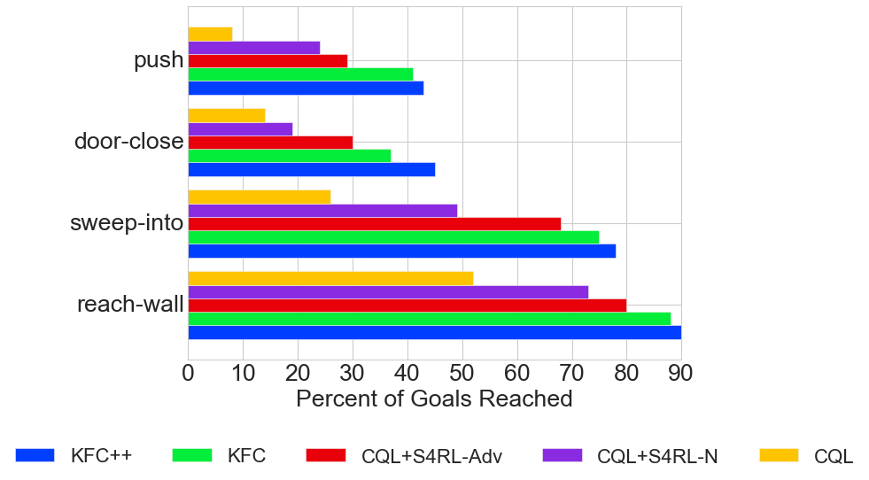
(a) MetaWorld Environments

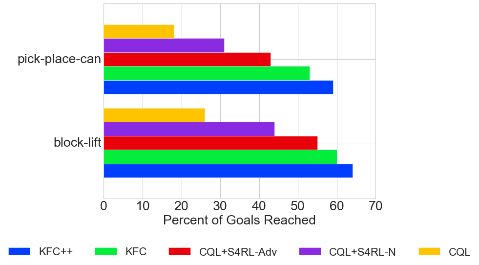
(b) RoboSuite Environments

Figure 2: Results on challenging dexterous robotics environments using data collected using a similar strategy as S4RL (Sinha et al., 2021). We report the $\%$ of goals that the agent is able to reach during evaluation, where the goal is set by the environments. We see that KFC and KFC++ consistently outperforms both CQL and the two best-performing S4RL variants.

4.1 D4RL benchmarks

We present results in the benchmark D4RL test suite and report the normalized return in Table 1. We see that both KFC and KFC++ consistently outperform both the baseline CQL and S4RL across multiple tasks and data distributions. Outperforming S4RL-variants on various different types of environments suggests that KFC and KFC++ fundamentally improves the data augmentation strategies discussed in S4RL.

KFC-variants also improve the performance of learned agents on challenging environments such as antmaze: which requires hierarchical planning, kitchen and adroit tasks: which are sparse reward and have large action spaces. Similarly, KFC-variants also perform well on difficult data distributions such as “medium-replay”: which is collected by simply using all the data that the policy encountered while training base SAC policy, and “-human” which is collected using human demonstrations on robotic tasks which results in a non-Markovian behaviour policy (more details can be found in the D4RL manuscript (Fu et al., 2021)).

Furthermore, to our knowledge, the results for KFC++ are state-of-the-art in model-free policy learning from D4RL datasets for most environments and data distributions. We do note that S4RL outperforms KFC on the “-random” split of the data distributions, which is expected as KFC depends on learning a simple dynamics model of the data to use to guide the data augmentation strategy. Since the “-random” split consists of random actions in the environment, our simple model is unable to learn a useful dynamics model. For ablation studies see appendix D.

4.2 Metaworld and Robosuite benchmarks

To further test the ability of KFC, we perform additional experiments on challenging robotic tasks. Following (Sinha et al., 2021), we perform additional experiments with 4 MetaWorld environments (Yu et al., 2019) and 2 RoboSuite environments (Zhu et al., 2020). We followed the same method to collect the data as described in Appendix F of S4RL (Sinha et al., 2021), and report the mean percent of goals reached, where the condition of reaching the goal is defined by the environment.

We report the results in Figure 2, where we see that by using KFC to guide the data augmentation strategy for a base CQL agent, we are able to learn an agent that performs significantly better. Furthermore, we see that for more challenging tasks such as “push” and “door-close” in the MetaWorld, KFC++ outperforms the base CQL algorithm and the S4RL agent by a considerable margin. This further highlights the ability of KFC to guide the data augmentation strategy.

5 Related works

The use of data augmentation techniques in Q-learning has been discussed recently (Laskin et al., 2020a, b; Sinha et al., 2021). In particular, our work shares strong parallels with (Sinha et al., 2021). Our modification of the policy evaluation step of the CQL algorithm (Kumar et al., 2020) is analogous to the one in Sinha et al. (2021). However, the latter randomly augments the data while our augmentation framework is based on symmetry state shifts. Regarding the connection to world models (Ha & Schmidhuber, 2018) a few comments in order. Here a VAE is used to decode the state information while a recurrent separate neural network predicts future states. Their latent representation is not of Koopman type. Also no symmetries and data-augmentations are derived.

Algebraic symmetries of the state-action space in Markov Decision Processes (MDP) originate (Balaraman & Andrew, 2004) an were discussed recently in the context of RL in (van der Pol et al., 2020). Their goal is to preserve the essential algebraic homomorphism symmetry structure of the original MDP while finding a more compact representation. The symmetry maps considered in our work are more general and are utilized in a different way. Symmetry-based representation learning (Higgins et al., 2018) refers to the study of symmetries of the environment manifested in the latent representation. The symmetries in our case are derived form the Koopman operator not the latent representation directly. In (Caselles-Dupré et al., 2019) the authors discuss representation learning of symmetries (Higgins et al., 2018) allowing for interactions with the environment. A Forward-VAE model which is similar to our Koopman-Forward VAE model is employed. We provide theoretical results on how to derive explicit symmetries of the dynamical systems as well as their utilisation for state-shifts.

In (Sinha et al., 2020) symmetries are used to extend the Koopman operator from a local to a global description. Neither action-equivariant dynamical control systems nor data augmentation is discussed. In (Salova et al., 2019) the imprint of known symmetries on the block-diagonal Koopman space representation for non-control dynamical systems is discussed. This is close to the spirit of disentanglement (Higgins et al., 2018). Our results are on control setups and deriving symmetries.

On another front, the application of Koopman theory in control or reinforcement learning has also been discussed recently. For example, (Li et al., 2020) propose to use compositional Koopman operators using graph neural networks to learn dynamics that can quickly adapt to new environments of unknown physical parameters and produce control signals to achieve a specified goal. (Kaiser et al., 2021) discuss the use of Koopman eigenfunction as a transformation of the state into a globally linear space where the classical control techniques is applicable. (Iwata & Kawahara, 2021) propose a framework for policy learning based on linear quadratic regulator in a space where the Koopman operator is defined. And, (Ohnishi et al., 2021) discuss a method of controlling nonlinear systems via the minimization of the Koopman spectrum cost: A cost over the Koopman operator of the controlled dynamics. However, to the best of our knowledge, this paper is the first to discuss Koopman latent space for data augmentation.

The study of Bisimulation metrics of action-state spaces has lead to performance improvements of Q-learning algorithms (Gelada et al., 2019; Zhang et al., 2021). We do not alter the metric of the action-state space as well do not take the reward into consideration. It would be interesting to study the KFC-algorithm trained on a Bisimulation metric space.

6 Conclusions

In this work we have proposed a symmetry-based data augmentation technique derived from a Koopman latent space representation. It enables a principled extension of offline RL datasets describing dynamical systems. The approach is based on our theoretical results on symmetries of dynamical control systems and symmetry shifts of data. Both hold for systems with differentiable state transitions and with a Bilinearisation model for the Koopman operator. However, the empirical results show that the framework is successfully applicable beyond those limitations.

We empirically evaluated our method on several benchmark offline reinforcement learning tasks D4RL, Metaworld and Robosuite and find that by using our framework we consistently improve the state-of-the-art of model-free Q-learning algorithms. Our framework is naturally applicable to model-based approaches and thus such an extension of our study would be of great interest.

Acknowledgments

This work was supported by JSPS KAKENHI (Grant Number JP22H00516), and JST CREST (Grant Number JPMJCR1913). And, we would like to thank Y. Nishimura for technical supports.

Appendix A Koopman theory and Symmetries

This section provides some additional introductory material on Koopman theory as well as a more detailed presentation of our results on symmetries of dynamical systems.

In general, a symmetry group $\Sigma$ of the state space may be any subgroup of the group of isometrics of the Euclidean space. We consider Euclidean state spaces and in particular, $\Sigma$ invariant compact subsets thereof.

Definition A.1 (Equivariant Dynamical System).

Consider the dynamical system $\dot{s}=f(s)$ and let $\Sigma$ be a group acting on the state-space $\mathcal{S}$. Then the system is called $\Sigma$-equivariant if $f(\sigma\cdot s)=\sigma\cdot f(s)\;,\;\;\text{for}\;s\in\mathcal{S}\;,\;\;\forall\sigma\in\Sigma$. For a discrete time dynamical system $s_{t+1}=F(s_{t})$ one defines equivariance analogously, namely if $F(\sigma\cdot s_{t})=\sigma\cdot F(s_{t})$ , for $\;s_{t}\in\mathcal{S}\;,\;\;\forall\sigma\in\Sigma$.

A system of ODEs may be represented by the set of its solutions which are locally connected by Lie Groups.

Definition A.2 (Symmetries of ODEs).

A symmetry of a system of ODEs on a locally-smooth structure is a locally-defined diffeomorphism that maps the set of all solutions to itself.

Definition A.3 (Local Lie Group).

A parametrized set of transformations $\sigma^{\epsilon}:\mathcal{S}\to\mathcal{S}$ with $s\mapsto\tilde{s}(s,\epsilon)$ for $\epsilon\in(\epsilon_{low},\epsilon_{high})$ where $\epsilon_{low}<0<\epsilon_{high}$ is a one-parameter local Lie group if

1. $\sigma^{0}$ is the identity map; for $\epsilon=0$ such that $\tilde{s}(s,0)=s$.

2. $\sigma^{\epsilon_{1}}\sigma^{\epsilon_{2}}=\sigma^{\epsilon_{2}}\sigma^{\epsilon_{1}}=\sigma^{\epsilon_{1}+\epsilon_{2}}$ for every $|\epsilon_{1}|,|\epsilon_{2}|\ll 1$.

3. $\tilde{s}(s,\epsilon)$ admits a Taylor series expansion in $\epsilon$; in a neighbourhood of $s$ determined by $\epsilon=0$ as $\tilde{s}(s,\epsilon)=s+\epsilon\,\zeta(s)+\mathcal{O}(\epsilon^{2})$.

The Koopman operator of equivariant dynamical system is reviewed in the following .

Lemma A.4.

The map $\ast:\Sigma\times\mathscr{K}(\mathcal{S})\rightarrow\mathscr{K}(\mathcal{S})$ given by $(\sigma\ast g)(s)\longmapsto g(\sigma^{-1}\cdot s)$ defines a group action on the Koopman space of observables $\mathscr{K}(\mathcal{S})$.

Theorem A.5.

Let $\mathcal{K}$ be the Koopman operator associated with a $\Sigma$-equivariant system $s_{t+1}=F(s_{t})$. Then

$$[\sigma\ast(\mathcal{K}g)](s)=[\mathcal{K}(\sigma\ast g)](s)\;\;.$$ (20)

Theorem A.5 states that for a $\Sigma$-equivariant system any symmetry transformation commutes with the Koopman operator. For the proof see (Sinha et al., 2020).

Let us next turn to the case relevant for RL, namely control systems. In the remainder of this section we focus on dynamical systems given as in Eq. (6) and Eq. (9).

Definition A.6 (Action Equivariant Dynamical System).

Let $\bar{\Sigma}$ be a group acting on the state-action-space $\mathcal{S}\times\mathcal{A}$ of a general control system as in Eq. (6) such that it acts as the identity operation on $\mathcal{A}$ i.e. $\sigma\cdot(s_{t},a_{t})=(\sigma|_{\mathcal{S}}\cdot s_{t},a_{t})\;,\;\;\forall\sigma\in\bar{\Sigma}\;\;.$ Then the system is called $\bar{\Sigma}$-action-equivariant if $\forall\sigma\in\bar{\Sigma}$

$$F(\sigma\cdot(s_{t},a_{t}))=\sigma|_{\mathcal{S}}\cdot F(s_{t},a_{t})\;,\;\;\text{for}\;(s_{t},a_{t})\in\mathcal{S}\times\mathcal{A}\;.$$ (21)

Lemma A.7.

The map $\bar{\ast}:\bar{\Sigma}\times\mathscr{K}(\mathcal{S}\times\mathcal{A})\rightarrow\mathscr{K}(\mathcal{S}\times\mathcal{A})$ given by $(\sigma\bar{\ast}g)(s,a)\longmapsto g(\sigma^{-1}\cdot s,a)$ defines a group action on the Koopman space of observables $\mathscr{K}(\mathcal{S}\times\mathcal{A})$.

Theorem A.8.

A Koopman operator $\mathcal{K}$ of a $\bar{\Sigma}$-action-equivariant system $s_{t+1}=F(s_{t},a_{t})$ satisfies

$$[\sigma\bar{\ast}(\mathcal{K}g)](s_{t},a_{t})=[\mathcal{K}(\sigma\bar{\ast}g)](s_{t},a_{t})\;\;.$$ (22)

In particular, it is easy to see that the biliniarisation in Eq. (9) is $\Sigma$-action-equivariant if $f_{i}(\sigma|_{\mathcal{S}}\cdot s)=\sigma|_{\mathcal{S}}\cdot f_{i}(s)\;,\;\;\forall i=0,\dots,m$. Let us thus turn our focus on the relevant case of a control system $s_{t+1}=\tilde{F}(s_{t},a_{t})$ which admits a Koopman operator description as

$$g(s_{t+1})=\mathcal{K}(a_{t})g(s_{t})\;,\;\;\text{for}\;a_{t}\in\mathcal{A}\,,\;\forall g\in\mathscr{K}(\mathcal{S})\;\;,$$ (23)

where $\{\mathcal{K}(a)\}_{a\in\mathcal{A}}$ is a family of operators with analytical dependence on $a\in\mathcal{A}$. Note that the bilinearisation in Eq. (9) is a special case of Eq. (13). Furthermore, let $\{U(a)\}_{a\in\mathcal{A}}$ be a family of invertible operators s.t. $U(a):\mathscr{K}(\mathcal{S})\to\mathscr{F}(\mathcal{S}\times\mathcal{A})$ is a mapping to the (Banach) space of eigenfunctions $\mathscr{F}(\mathcal{S}\times\mathcal{A})$ with eigenfunctions $\varphi(s,a):=U(a)g(s)$ which obeys $U(a)\mathcal{K}(a)U(a)^{-1}=\Lambda(a)$, with $\Lambda(a)\varphi(s,a)=\lambda_{\varphi}(a)\varphi(s,a)$ and where $\lambda_{\varphi}(a):\mathcal{A}\to\mathbb{R}$. The existence of such operators on an infinite dimensional space requires the Koopman operator in Eq. (13) to be self-adjoint or a finite-dimensional (approximate) matrix representation to be diagonalizable.

Lemma A.9.

The map $\hat{\phi}:\bar{\Sigma}\times\mathscr{K}(\mathcal{S})\times\{U(a)\}_{a\in\mathcal{A}}\rightarrow\mathscr{K}(\mathcal{S})$ given by

$$(\sigma_{a}\hat{\ast}g)(s)\longmapsto\Big{(}U^{-1}(a)\big{(}\sigma\bar{\ast}(U(a)g)\big{)}\Big{)}(s)=g(\sigma^{-1}\cdot s)\;\;,$$ (24)

defines a group action on the Koopman space of observables $\mathscr{K}(\mathcal{S})$. Where $\bar{\ast}$ is defined analog to Lemma A.7 but acting on $\mathscr{F}(\mathcal{S}\times\mathcal{A})$ instead of $\mathscr{K}(\mathcal{S}\times\mathcal{A})$ by $(\sigma\bar{\ast}\varphi)(s,a)\longmapsto\varphi(\sigma^{-1}\cdot s,a)$. We refer to a control system in Eq. (23) admitting a $\hat{\phi}$-symmetry as $\hat{\Sigma}$-action-equivariant.

Theorem A.10.

Let $s_{t+1}=\tilde{F}(s_{t},a_{t})$ be a $\hat{\Sigma}$-action-equivariant control system with a symmetry action as in Lemma A.9 which furthermore admits a Koopman operator representation as

$$\vspace{-0.05cm}g(s_{t+1})=\mathcal{K}(a_{t})g(s_{t})\;,\;\;\text{for}\;a_{t}\in\mathcal{A}\,,\;\forall g\in\mathscr{K}(\mathcal{S})\;\;.$$ (25)

Then

$$\big{[}\sigma_{a_{t}}\hat{\ast}\big{(}\mathcal{K}(a_{t})g\big{)}\big{]}(s_{t})=\big{[}\mathcal{K}(a_{t})\,\big{(}\sigma_{a_{t}}\hat{\ast}g\big{)}\big{]}(s_{t})\;\;.$$ (26)

Moreover, a control system obeying equations 25 and 26 is $\hat{\Sigma}$-action-equivariant locally if $g^{-1}$ exists for a neighborhood of $s_{t}$, i.e. then $\sigma\cdot\tilde{F}(s_{t},a_{t})=\tilde{F}(\sigma\cdot(s_{t},a_{t}))$.

To allow an easier transition to the empirical section we introduce the notation $E:\mathcal{S}\to\mathscr{K}(S)$ and $D:\mathscr{K}(S)\to\mathcal{S}$ denote the $\mathcal{C}^{1}$-differentiable encoder and decoder to and from the finite-dimensional Koopman space approximation, respectively, i.e. $E\circ D=D\circ E=id$. Data-points may be shifted by symmetry transformations of solutions of ODEs as discussed next.

Theorem A.11.

Let $s_{t+1}=\tilde{F}(s_{t},a_{t})$ be a control system as in Eq. (25) and $\sigma_{a_{t}}$ an operator obeying Eq. (26). Then $\sigma_{a_{t}}^{\epsilon}:\big{(}s_{t},s_{t+1},a_{t}\big{)}\longmapsto\big{(}\tilde{s}_{t},\tilde{s}_{t+1},a_{t}\big{)}$ with

$$\tilde{s}_{t} = D\Big{(}\,\big{(}\mathds{1}\;+\;\epsilon\,\sigma_{a_{t}}\big{)}\hat{\ast}E(s_{t})\Big{)}\;,$$ (27)

$$\tilde{s}_{t+1} = D\Big{(}\,\big{(}\mathds{1}\;+\;\epsilon\,\sigma_{a_{t}}\big{)}\hat{\ast}E(s_{t+1})\Big{)}\;\;\,$$

is a one-parameter local Lie symmetry group of ODEs. In other words one can use a symmetry transformation to shift both $s_{t}$ as well as $s_{t+1}$ such that $\tilde{s}_{t+1}=\tilde{F}(\tilde{s}_{t},a_{t})$.

No assumptions on the Koopman operator are imposed. Moreover, note that the equivalent theorem holds when $\epsilon\,\sigma_{a_{t}}\to\sum_{I=1}\epsilon_{I}\,\sigma^{I}_{a_{t}}$ to be a local N-parameter Lie group.

Additional Remarks. Let us re-evaluate some information given on the operators used previously. Let $\{U(a)\}_{a\in\mathcal{A}}$ be a family of invertible operators s.t. $U(a):\mathscr{K}(\mathcal{S})\to\mathscr{F}(\mathcal{S}\times\mathcal{A})$ is a mapping to the (Banach) space of eigenfunctions $\varphi(s,a):=U(a)g(s)\in\mathscr{F}(\mathcal{S}\times\mathcal{A})$. Which moreover obeys

$$U(a)\mathcal{K}(a)U(a)^{-1} = \Lambda(a),\;\;\text{with}$$ (28)

$$\Lambda(a)\varphi(s,a) = \lambda_{\varphi}(a)\varphi(s,a)\;\;,$$

and where $\lambda_{\varphi}(a):\mathcal{A}\to\mathbb{R}$. The existence of such operators puts further restriction on the Koopman operator in Eq. (13). However, as our algorithm employs the finite-dimensional approximation of the Koopman operator i.e. its matrix representation this amounts simple for $\mathcal{K}(a)$ to be diagonalizable and $U(a)$ is the matrix containing its eigen-vectors as columns. To evolve a better understanding on the required criteria for the infinite-dimensional case we employ an alternative formulation of the so called spectral theorem below.

Theorem A.12 (Spectral Theorem).

Let $\mathcal{K}$ be a bounded self-adjoint operator on a Hilbert space $\mathcal{H}$. Then there is a measure space $(\mathcal{S},\Sigma,\mu)$ and a real-valued essentially bounded measurable function $\lambda$ on $\mathcal{S}$ and a unitary operator $U:\mathcal{H}\to L^{2}_{\mu}(\mathcal{S})$ i.e. $U^{\ast}U=U\,U^{\ast}=id$ such that

$$U\,\Lambda\,U^{\ast}=\mathcal{K}\;,\;\;\text{with}\;\;\big{[}\Lambda\varphi\big{]}(s)=\lambda(s)\varphi(s)\;\;.$$ (29)

In other words every bounded self-adjoint operator is unitarily equivalent to a multiplication operator. In contrast to the finite-dimensional case we need to slightly alter our criteria to $U(a)\mathcal{K}(a)U(a)^{-1}=\Lambda(a)$, with $\Lambda(a)\varphi(s,a)=\lambda_{\varphi}(a,s)\varphi(s,a)$ and where $\lambda_{\varphi}(s,a):\mathcal{S}\times\mathcal{A}\to\mathbb{R}$. Concludingly, a sufficient condition for our criteria to hold in terms of operators on Hilbert spaces is that the Koopman operator $\mathcal{K}(a)$ is self-adjoint i.e. that

$$\mathcal{K}(a)=\mathcal{K}(a)^{\ast}\;\;.$$ (30)

Appendix B Proofs

In this section we provide the proofs of the theoretical results of Section 3.

Proof of Lemma A.4 and Theorem A.5

The proofs of the lemma as well as the theorem can be found in (Sinha et al., 2020).

Proof of Lemma 3.5:

We aim to show that map $\bar{\ast}:\bar{\Sigma}\times\mathscr{K}(\mathcal{S}\times\mathcal{A})\rightarrow\mathscr{K}(\mathcal{S}\times\mathcal{A})$ given by $(\sigma\bar{\ast}g)(s,a)\longmapsto g(\sigma^{-1}\cdot s,a)$ defines a group action on the Koopman space of observables $\mathscr{K}(\mathcal{S}\times\mathcal{A})$, where $\bar{\Sigma}$ defines the symmetry group of definition 3.4. Firstly, let $g\in\mathscr{K}(\mathcal{S}\times\mathcal{A})$ and $\sigma_{0}\in\bar{\Sigma}$ be the identity element, then we see that it provides existence of an identity element of $\bar{\ast}$ by

$$(\sigma_{0}\bar{\ast}g)(s,a)=g\big{(}\sigma_{0}^{-1}\cdot s,a\big{)}=g(s,a)\;\;.$$

Secondly, let $\sigma_{1},\sigma_{2}\in\bar{\Sigma}$ and $\odot$ denoting the group operation i.e. $\sigma_{1}\odot\sigma_{2}=\sigma_{3}\in\bar{\Sigma}$. Then

$$\Big{(}\sigma_{2}\bar{\ast}\big{(}\sigma_{1}\bar{\ast}g\big{)}\Big{)}(s,a) = \sigma_{2}\bar{\ast}\Big{(}g\big{(}\sigma_{1}^{-1}\cdot s,a\big{)}\Big{)}$$ (31)

$$= g\big{(}\sigma_{2}^{-1}\cdot(\sigma_{1}^{-1}\cdot s),a\big{)}$$

$$= g\big{(}(\sigma_{2}^{-1}\odot\sigma_{1}^{-1})\cdot s),a\big{)}$$

$$\stackrel{{\scriptstyle(I)}}{{=}} g\big{(}(\sigma_{1}\odot\sigma_{2})^{-1}\cdot s,a\big{)}$$

$$= \Big{(}\big{(}\sigma_{1}\odot\sigma_{2}\big{)}\bar{\ast}g\Big{)}(s,a)$$

$$= \Big{(}\sigma_{3}\bar{\ast}g\Big{)}(s,a)\;\;,$$

where in $(I)$ we have used the invertibility of the group property of $\bar{\Sigma}$. Lastly it follows analogously that for $\sigma,\sigma^{-1}\in\bar{\Sigma}$ that

$$\Big{(}\sigma\bar{\ast}\big{(}\sigma^{-1}\bar{\ast}g\big{)}\Big{)}(s,a) = \Big{(}\big{(}\sigma^{-1}\odot\sigma\big{)}\bar{\ast}g\Big{)}(s,a)$$

$$= \Big{(}\sigma_{0}\bar{\ast}g\Big{)}(s,a)=g(s,a)\;\;.$$

Thus the existence of an inverse is established which concludes to show the group property of $\bar{\ast}$.

Proof of Theorem 3.6:

We aim to show that with $\mathcal{K}$ being the Koopman operator associated with a $\bar{\Sigma}$-action-equivariant system $s_{t+1}=F(s_{t},a_{t})$. Then

$$\Big{[}\,\sigma\bar{\ast}\big{(}\mathcal{K}g\big{)}\,\Big{]}(s,a)=\Big{[}\,\mathcal{K}\big{(}\sigma\bar{\ast}g\big{)}\Big{]}(s,a)\;\;.$$

First of all note that by the definition of the Koopman operator of non-affine control systems it obeys

$$[\mathcal{K}g](s_{t},a_{t})=g(F(s_{t},a_{t}),a_{t+1})\;\;.$$

Using the latter one thus infers that

$$\Big{[}\sigma\bar{\ast}\big{(}\mathcal{K}g\big{)}\Big{]}(s_{t},a_{t}) = \sigma\bar{\ast}g(F(s_{t},a_{t}),a_{t+1})$$

$$= g(\sigma^{-1}\cdot F(s_{t},a_{t}),a_{t+1})$$

$$\stackrel{{\scriptstyle(I)}}{{=}} g(F(\sigma^{-1}\cdot s_{t},a_{t}),a_{t+1})\,,$$

where in (I) we have used that it is a $\bar{\Sigma}$-action-equivariant system. Moreover, one finds that

$$g(F(\sigma^{-1}\cdot s_{t},a_{t}),a_{t+1}) = \mathcal{K}g(\sigma^{-1}\cdot s_{t},a_{t})$$

$$= \Big{[}\,\mathcal{K}\big{(}\sigma\bar{\ast}g\big{)}\,\Big{]}(s_{t},a_{t})\;\;,$$

which concludes the proof.

Proof of Lemma A.9:

We aim to show that the map $\hat{\phi}:\bar{\Sigma}\times\mathscr{K}(\mathcal{S})\times\{U(a)\}_{a\in\mathcal{A}}\rightarrow\mathscr{K}(\mathcal{S})$ given by

$$\big{(}\sigma_{a}\hat{\ast}g\big{)}(s)\longmapsto\Big{(}U^{-1}(a)\big{(}\sigma\bar{\ast}(U(a)g)\big{)}\Big{)}(s)=g\big{(}\sigma^{-1}\cdot s\big{)}\;\;,$$

defines a group action on the Koopman space of observables $\mathscr{K}(\mathcal{S})$. Where $\bar{\ast}$ is defined analog to Lemma 3.5 but acting on $\mathscr{F}(\mathcal{S}\times\mathcal{A})$ instead of $\mathscr{K}(\mathcal{S}\times\mathcal{A})$ by $(\sigma\bar{\ast}\varphi)(s,a)\longmapsto\varphi(\sigma^{-1}\cdot s,a)$. First of all note that

$$\Big{(}U^{-1}(a)\big{(}\bar{\sigma}\ast(U(a)g)\big{)}\Big{)}(s) = U^{-1}(a)\big{(}\bar{\sigma}\ast\varphi(s,a)\big{)}$$ (35)

$$= U^{-1}(a)\varphi\big{(}\sigma^{-1}\cdot s,a\big{)}$$

$$= g\big{(}\sigma^{-1}\cdot s\big{)}$$

We proceed analogously as in the proof of Lemma 3.5 above. Firstly, let $g\in\mathscr{K}(\mathcal{S})$ and $\sigma_{0}\in\bar{\Sigma}$ be the identity element then on infers from Eq. (35) that it provides existence of an identity element of $\hat{\phi}$ by

$$(\sigma_{a,0}\hat{\ast}g)(s)=g\big{(}\sigma_{0}^{-1}\cdot s\big{)}=g(s)\;\;,$$

where we have used the notation $\text{for}\;\;i=0,\dots$

$$(\sigma_{a,i}\hat{\ast}g)(s)=\Big{(}U^{-1}(a)\big{(}\sigma_{i}\bar{\ast}(U(a)g)\big{)}\Big{)}(s)\;,\;\;.$$

Secondly, let $\sigma_{1},\sigma_{2}\in\bar{\Sigma}$ and $\odot$ denoting the group operation i.e. $\sigma_{1}\odot\sigma_{2}=\sigma_{3}\in\bar{\Sigma}$. Then

$$\Big{(}\sigma_{a,2}\hat{\ast}\big{(}\sigma_{a,1}\hat{\ast}g\big{)}\Big{)}(s) = \sigma_{a,2}\hat{\ast}\Big{(}g\big{(}\sigma_{1}^{-1}\cdot s\big{)}\Big{)}$$

$$= g\big{(}\sigma_{2}^{-1}\cdot(\sigma_{1}^{-1}\cdot s)\big{)}$$

$$= g\big{(}(\sigma_{2}^{-1}\odot\sigma_{1}^{-1})\cdot s\big{)}$$

$$\stackrel{{\scriptstyle(I)}}{{=}} g\big{(}(\sigma_{1}\odot\sigma_{2})^{-1}\cdot s\big{)}$$

$$= g\big{(}\sigma_{3}^{-1}\cdot s\big{)}$$

$$= \Big{(}\sigma_{a,3}\bar{\ast}g\Big{)}(s)\;\;,$$

where in $(I)$ we have used the invertibility of the group property of $\Sigma$. Lastly, it follows analogously that for $\sigma,\sigma^{-1}\in\bar{\Sigma}$ that

$$\Big{(}\sigma\hat{\ast}\big{(}\sigma^{-1}\hat{\ast}g\big{)}\Big{)}(s) = \Big{(}\big{(}\sigma^{-1}\odot\sigma\big{)}\hat{\ast}g\Big{)}(s)$$

$$= \Big{(}\sigma_{0}\hat{\ast}g\Big{)}(s)=g(s)\;\;.$$

Thus the existence of an inverse is established which concludes to show the group property of $\hat{\phi}$.

Proof of Theorem 3.8:

We aim to show twofold.

$\Longrightarrow$:

Firstly, that with $s_{t+1}=\tilde{F}(s_{t},a_{t})$ be a $\hat{\Sigma}$-action-equivariant control system with a symmetry action as in Lemma A.9 which furthermore admits a Koopman operator representation as

$$g(s_{t+1})=\mathcal{K}(a_{t})g(s_{t})\;,\;\;\text{for}\;a_{t}\in\mathcal{A}\,,\;\forall g\in\mathscr{K}(\mathcal{S})\;\;.$$

Then

$$\Big{[}\sigma_{a_{t}}\hat{\ast}\big{(}\mathcal{K}(a_{t})g\big{)}\Big{]}(s_{t})=\Big{[}\mathcal{K}(a_{t})\,\big{(}\sigma_{a_{t}}\hat{\ast}g\big{)}\Big{]}(s_{t})\;\;.$$

$\Longleftarrow$:

Secondly, the converse. Namely, if a control system $s_{t+1}=\tilde{F}(s_{t},a_{t})$ obeys Eqs. (14) and (15), then it is $\hat{\Sigma}$-action-equivariant, i.e. $\sigma\cdot\tilde{F}(s_{t},a_{t})=\tilde{F}(\sigma\cdot(s_{t},a_{t}))$. For notational simplicity we drop the subscripts referring to time in the remainder of this proof i.e.  $s_{t}\to s$ and $a_{t}\to a$.

Let us start with the first implication i.e. $\Longrightarrow$.

First of all note that by the definition of the Koopman operator one has

$$\big{[}\mathcal{K}(a)g\big{]}(s)=g\big{(}\tilde{F}(s,a)\big{)}\;\;.$$

Using the latter one infers that

$$\Big{[}\sigma_{a}\hat{\ast}\big{(}\mathcal{K}(a)g\big{)}\Big{]}(s) = \sigma_{a}\hat{\ast}g(\tilde{F}(s,a))\;\;,$$

$$= U^{-1}(a)\Big{(}\sigma\bar{\ast}\big{(}U(a)g\big{(}\tilde{F}(s,a)\big{)}\big{)}\Big{)}\;\;,$$

$$= U^{-1}(a)\Big{(}\sigma\bar{\ast}\varphi\big{(}\tilde{F}(s,a),a\big{)}\Big{)}\;\;,$$

$$= U^{-1}(a)\Big{(}\varphi\big{(}\sigma^{-1}\cdot\tilde{F}(s,a),a\big{)}\big{)}\Big{)}\;\;,$$

$$= U^{-1}(a)\Big{(}\varphi\big{(}\tilde{F}\big{(}\sigma^{-1}\cdot s,a\big{)},a\big{)}\big{)}\Big{)}\;\;,$$

$$= g\big{(}\tilde{F}\big{(}\sigma^{-1}s,a\big{)}\big{)}\;\;.$$

Moreover, one derives that

$$g\big{(}\tilde{F}\big{(}\sigma^{-1}s,a\big{)}\big{)} = \mathcal{K}(a)g\big{(}\sigma^{-1}s\big{)}\;\;,$$

$$= \mathcal{K}(a)\,\underbrace{U^{-1}(a)\,U(a)}_{=id}g\big{(}\sigma^{-1}s\big{)}\;\;,$$

$$= \mathcal{K}(a)\,U^{-1}(a)\,\varphi\big{(}\sigma^{-1}s,a\big{)}\;\;,$$

$$= \mathcal{K}(a)\Big{(}\,U^{-1}(a)\,\big{(}\sigma\bar{\ast}\varphi\big{(}s,a\big{)}\big{)}\Big{)}\;\;,$$

$$= \mathcal{K}(a)\Big{(}\,U^{-1}(a)\,\big{(}\sigma\bar{\ast}\big{(}U(a)g(s)\big{)}\big{)}\Big{)}\;\;,$$

$$= \Big{[}\mathcal{K}(a)\,\big{(}\sigma_{a}\hat{\ast}g\big{)}\Big{]}(s)\;\;,$$

which concludes the proof of the first part of the theorem. Let us next show the converse implication i.e. $\Longleftarrow$. For this case it is practical to use the discrete time-system notation explicitly. Let $\sigma\in\Sigma$ be a symmetry of the state-space and be $\tilde{s}_{t}=\sigma\cdot s_{t}$ and $\tilde{s}_{t+1}=\sigma\cdot s_{t+1}$ the $\sigma$-shifted states. Then

$$g\big{(}s_{t+1}\big{)} = g\big{(}\tilde{F}(s_{t},a_{t})\big{)}\;\;,$$

$$= \mathcal{K}(a_{t})\,g(s_{t})\;\;,$$

$$= \mathcal{K}(a_{t})\,g\big{(}\sigma^{-1}\cdot\tilde{s}_{t}\big{)}\;\;,$$

$$= \mathcal{K}(a_{t})\Big{(}\sigma_{a}\hat{\ast}g\big{(}\tilde{s}_{t}\big{)}\Big{)}\;\;,$$

$$= \Big{[}\mathcal{K}(a_{t})\big{(}\sigma_{a}\hat{\ast}g\big{)}\Big{]}(\tilde{s}_{t})\;\;,$$

$$\stackrel{{\scriptstyle(I)}}{{=}} \Big{[}\sigma_{a}\hat{\ast}\big{(}\mathcal{K}(a_{t})g\big{)}\Big{]}(\tilde{s}_{t})\;\;,$$

where in (I) we have used that the symmetry operator commutes with the Koopman operator. Thus in particular

$$\sigma_{a}^{-1}\hat{\ast}g\big{(}s_{t+1}\big{)} = \Big{[}\sigma_{a}^{-1}\hat{\ast}\big{(}\sigma_{a}\hat{\ast}\big{(}\mathcal{K}(a_{t})g\big{)}\big{)}\Big{]}(\tilde{s}_{t})$$ (38)

$$\stackrel{{\scriptstyle Lemma\;\ref{lem:hatphiA}}}{{=}} \Big{[}\mathcal{K}(a_{t})g\Big{]}(\tilde{s}_{t})\;\;,$$

Moreover, one finds that

$$\sigma_{a}^{-1}\hat{\ast}g\big{(}s_{t+1}\big{)} = g\Big{(}\big{(}\sigma^{-1}\big{)}^{-1}\cdot s_{t+1}\Big{)}$$

$$= g\big{(}\sigma\cdot s_{t+1}\big{)}=g\big{(}\tilde{s}_{t+1}\big{)}\;\;,$$

from which one concludes that

$$g(\tilde{s}_{t+1})=\big{[}\mathcal{K}(a_{t})g\big{]}(\tilde{s}_{t})=g\big{(}\tilde{F}(\tilde{s}_{t},a_{t})\big{)}\;\;.$$

Finally, we use the invertibility of the Koopman space observables i.e. $g^{-1}(g(s))=s$ to infer

$$\tilde{s}_{t+1}=\tilde{F}(\tilde{s}_{t},a_{t})\;\;.$$

However, in general $s$ the Koopman space observables are not invertible globally. The "inverse function theorem" guarantees the existence of a local inverse if $g(s)$ is $\mathcal{C}^{1}$ differentiable for maps between manifolds of equal dimensions; see any classical reference/text-book on differential calculus. However, we assume inevitability locally.

$$\tilde{s}_{t+1}=\sigma\cdot s_{t+1}\;\; \Rightarrow \;\;\tilde{F}(\tilde{s}_{t},a_{t})=\sigma\cdot\tilde{F}(s_{t},a_{t})\;\;$$

$$\Rightarrow \tilde{F}(\sigma\cdot s_{t},a_{t})=\sigma\cdot\tilde{F}(s_{t},a_{t})\;\;,$$

which at last concludes our proof of the second part of the theorem.

Extension of Theorem 3.9:

Moreover, one may account for practical limitations i.e. an error by the assumption $[\sigma_{a_{t}}^{\epsilon},\mathcal{K}(a_{t})]=\epsilon_{a}\,\mathds{1}$. One then finds that $\tilde{s}_{t+1}=\tilde{F}(\tilde{s}_{t},a_{t})+\mathcal{O}(\epsilon_{a})$. Thus the error becomes suppressed when $\epsilon_{a}\ll\epsilon$. The error may be due to practical limitations of capturing the true dynamics as well as the symmetry map.

Proof of Theorem 3.9:

We will show here theorem 3.9 as well as the extension mentioned in the paragraph prior to this proof. Let $s_{t+1}=\tilde{F}(s_{t},a_{t})$ be a $\hat{\Sigma}$-action-equivariant control system as in Theorem 3.8. For symmetry maps

$$\tilde{s}_{t} = D\Big{(}\,\big{(}\mathds{1}\;+\;\epsilon\,\sigma_{a_{t}}\big{)}\hat{\ast}E(s_{t})\Big{)}\;,\;\;$$ (41)

$$\tilde{s}_{t+1} = D\Big{(}\,\big{(}\mathds{1}\;+\;\epsilon\,\sigma_{a_{t}}\big{)}\hat{\ast}E(s_{t+1})\Big{)}\;\;.$$

we aim to show that one can use a symmetry transformation to shift both $s_{t}$ as well as $s_{t+1}$

$$\sigma_{a_{t}}^{\epsilon}:\;\;\big{(}s_{t},s_{t+1},a_{t}\big{)}\;\;\longmapsto\;\;\big{(}\tilde{s}_{t},\tilde{s}_{t+1},a_{t}\big{)}$$ (42)

such that

$$\tilde{s}_{t+1}=\tilde{F}(\tilde{s}_{t},a_{t})\;.$$ (43)

From Eq. (41) and the definition of the Koopman operator one infers that

$$\tilde{s}_{t+1}=D\Big{(}\ \sigma_{a_{t}}\hat{\ast}E(s_{t+1})\Big{)}=D\Big{(}\ \sigma_{a_{t}}\hat{\ast}\mathcal{K}(a_{t})E(s_{t})\Big{)}\;\;.$$ (44)

By using that $[\sigma_{a_{t}},\mathcal{K}(a_{t})]=0$ and Eq. (41) one finds that

$$\tilde{s}_{t+1} = D\Big{(}\ \mathcal{K}(a_{t})\sigma_{a_{t}}\hat{\ast}E(s_{t})\Big{)}$$

$$= D\Big{(}\ \mathcal{K}(a_{t})\underbrace{E(D(}_{=\mathds{1}}\sigma_{a_{t}}\hat{\ast}E(s_{t})))\Big{)}$$

$$= D\Big{(}\ \mathcal{K}(a_{t})E(\tilde{s}_{t})\Big{)}\;\;,$$

which concludes the proof of the first part of the theorem with $\sigma_{a_{t}}\to(\mathds{1}\;+\;\epsilon\,\sigma_{a_{t}})$.
Local diffeomorphism. Per definition the maps $D,E$ are differentiable and invertible which implies that they provide a local diffeomorphism from and to Koopman-space. Also the linear map i.e. a matrix multiplication by $(\mathds{1}\;+\;\epsilon\,\sigma_{a_{t}})$ is a diffeomorphism. Thus the symmetry map $\sigma_{a_{t}}^{\epsilon}$ i.e. Eq. (16) constitutes a local diffeomorphism. The above proof culminating in Eq. (41) implies that we have a local diffeomorphism mapping solutions of the ODEs to solutions, thus a symmetry of the system of ODEs.
Limitations. However $D,E$ to be invertible is a strong assumption as it implies that the Koopman space approximation admit the same dimension as the state space. Note that however in practice as we only require $D\circ E\approx id$ one may choose other Koopman space dimensions.
Local Lie group. What is left to show is that the symmetry of the system of ODEs locally is a Lie group. In definition 3.3 we need to show points (1)-(3).

1. For $\epsilon=0$ one finds that $\sigma^{0}_{a_{t}}$ is the identity map i.e for such that

   $$\tilde{s}_{t}(s_{t},0)=D\big{(}(\mathds{1}\;+\;0\cdot\,\sigma_{a_{t}})E(s_{t})\big{)}=D(E(s_{t}))=s_{t}$$ (46)

2. $$\sigma^{\epsilon_{1}}\sigma^{\epsilon_{2}} = D\big{(}(\mathds{1}+\epsilon_{1}\sigma_{a_{t}})(\mathds{1}+\epsilon_{2}\sigma_{a_{t}})E(s_{t})\big{)}$$

   $$= D\big{(}(\mathds{1}+(\epsilon_{1}+\epsilon_{2})\sigma_{a_{t}}+\mathcal{O}(\epsilon_{1}\cdot\epsilon_{2}))E(s_{t})\big{)}$$

   $$= \sigma^{\epsilon_{1}+\epsilon_{2}}$$

   for every $|\epsilon_{1}|,|\epsilon_{2}|\ll 1$.

3. $\tilde{s}_{t}(s_{t},\epsilon)$ admits a Taylor series expansion in $\epsilon$, i.e. in a neighbourhood of $s$ determined by $\epsilon=0$. We may Taylor expand D around the point $E(s_{t})\equiv g$ as

   $$\tilde{s}_{t}(s_{t},\epsilon)=D(E(s_{t}))+\epsilon\sum_{I=1}^{N}(\sigma_{a_{t}}E(s_{t}))_{I}\frac{\partial D}{\partial g_{I}}+\mathcal{O}(\epsilon^{2})$$ (48)

   thus

   $$\tilde{s}_{t}(s_{t},\epsilon)=s_{t}+\epsilon\zeta(s_{t})+\mathcal{O}(\epsilon^{2})$$ (49)

   for $\zeta(s_{t})=\sum_{I=1}^{N}(\sigma_{a_{t}}E(s_{t}))_{I}\tfrac{\partial D}{\partial g_{I}}$.

4. The existence of an inverse element $(\sigma_{a_{t}}^{\epsilon})^{-1}=\sigma_{a_{t}}^{-\epsilon}$ follows from (1) and (2).

Numerical errors. Let us next turn to the second part of the theorem incorporating for practical numerical errors. We aim to show that under the assumption $[\sigma_{a_{t}}^{\epsilon},\mathcal{K}(a_{t})]=\epsilon_{a}\,\mathds{1}$ one finds $\tilde{s}_{t+1}=\tilde{F}(\tilde{s}_{t},a_{t})+\mathcal{O}(\epsilon_{a})$. Note that $\sigma_{a_{t}}\to(\mathds{1}\;+\;\epsilon\,\sigma_{a_{t}})$ admits an expansion in the parameter $\epsilon$. For $\epsilon\ll 1$ one can Taylor expand the differentiable functions $D,E$ to find that

$$\tilde{s}_{t}=s_{t}+\delta(\epsilon)\;,\;\;\text{with}\;\;\delta(\epsilon)=\epsilon\;\sum_{I}g^{\sigma}_{I}\frac{\partial D}{\partial g_{I}}\big{|}_{E(s_{t})}+\mathcal{O}(\epsilon^{2})\,,$$ (50)

where $g^{\sigma}=\,\sigma_{a_{t}}\hat{\ast}E(s_{t})$ and $g=E(s_{t})$, and with the index $I=1,\dots,N$. The analog expression holds for $t+1$ i.e. $\tilde{s}_{t+1}=s_{t+1}+\mathcal{O}(\epsilon)$. If $a_{t}=a_{t}(s_{t})$ is differentiable function of the states one may Taylor expand the Koopman operator using Eq. (50) as

$$K(a_{t}(\tilde{s}_{t})) = K(a_{t}(s_{t}))+\sum_{i}\sum_{n}\delta_{n}(\epsilon)\,a^{\prime}_{in}(s_{t})\,\mathcal{K}_{i}$$ (51)

$$= K(a_{t}(s_{t}))+\epsilon\,\Delta+\mathcal{O}(\epsilon^{2})\;\;.$$

where and $a^{\prime}_{in}(s_{t})=\tfrac{\partial a_{t}}{\partial_{s_{t,n}}}|_{s_{t}}$ and $n=1,\dots,dim(s_{t})$ and with

$$\Delta=\sum_{i}\sum_{n}\sum_{I}g^{\sigma}_{I}\frac{\partial D_{n}}{\partial g_{I}}\big{|}_{E(s_{t})}a^{\prime}_{in}(s_{t})\,\mathcal{K}_{i}\;\;.$$ (52)

However, by the definition of the symmetry map $a_{t}(\tilde{s}_{t})=a_{t}(s_{t})$, thus the Koopman operators in Eq. (51) match $\forall\epsilon$. By using the assumption on the error one infers from Eq. (44) that

$$\tilde{s}_{t+1} = D\Big{(}(\mathds{1}+\epsilon\sigma_{a_{t}})\hat{\ast}\mathcal{K}(a_{t})E(s_{t})\Big{)}$$

$$= D\Big{(}\big{(}\mathcal{K}(a_{t})+\epsilon_{a}\,\mathds{1}\big{)}\,(\mathds{1}+\epsilon\sigma_{a_{t}})\hat{\ast}E(s_{t})\Big{)}$$

$$= D\Big{(}\mathcal{K}(a_{t})(\mathds{1}+\epsilon\sigma_{a_{t}})\hat{\ast}E(s_{t})+\epsilon_{a}E(s_{t})+\mathcal{O}(\epsilon_{a}\epsilon)\Big{)}$$

$$= D\Big{(}\mathcal{K}(a_{t})E(\tilde{s}_{t})+\epsilon_{a}E(s_{t})+\mathcal{O}(\epsilon_{a}\epsilon)\Big{)}\;\;,$$

One may Taylor expand $D$ by making use of $\epsilon_{a}\ll 1$ as

$$\tilde{s}_{t+1}=D\big{(}\mathcal{K}(a_{t})E(\tilde{s}_{t})\big{)} + \epsilon_{a}\sum_{I}E_{I}(s_{t})\frac{\partial D}{\partial g_{I}}\Big{|}_{\mathcal{K}(a_{t})E(\tilde{s}_{t})}$$ (54)

$$+ \mathcal{O}(\epsilon_{a}\epsilon)+\mathcal{O}(\epsilon_{a}^{2})\;\;.$$

Thus under the assumption that the numerical error is given by a violation of the commutation relation one finds $\tilde{s}_{t+1}=\tilde{F}(\tilde{s}_{t},a_{t})+\mathcal{O}(\epsilon_{a})$ where

$$\epsilon_{a}\,\sum_{I}E_{I}(s_{t})\frac{\partial D}{\partial g_{I}}\Big{|}_{\mathcal{K}(a_{t})E(\tilde{s}_{t})}\sim\mathcal{O}(\epsilon_{a})\;\;.$$ (55)

By comparison with Eq. (50) one infers that the $\epsilon$-expansion is a good approximation to the real dynamic if $\epsilon_{a}\ll\epsilon$. This concludes the proof of theorem 3.9. Let us note that the proof for state shifts arising from a sum of symmetry transformations as

$$\tilde{s}_{t} = D\Big{(}\,\big{(}\mathds{1}\;+\;\sum_{I=1}^{N}\epsilon_{I}\,\sigma^{I}_{a_{t}}\big{)}\hat{\ast}E(s_{t})\Big{)}\;,$$ (56)

$$\tilde{s}_{t+1} = D\Big{(}\,\big{(}\mathds{1}\;+\;\sum_{I=1}^{N}\epsilon_{I}\,\sigma^{I}_{a_{t}}\big{)}\hat{\ast}E(s_{t+1})\Big{)}\;\;.$$

is completely analogous, and an analogous theorem holds. We choose the number of symmetries to run over the dimension of the Koopman latent space $N$ as it is relevant for the KFC++ setup.

Appendix C Implementation details

The Koopman forward model The KFC algorithm requires pre-training of a Koopman forward model $\mathcal{F}:\mathcal{S}\times\mathcal{A}\to\mathcal{S}$ as

$$\mathcal{F}^{c}(s_{t},a_{t})=\begin{cases}{\bf c=0\;\;\text{VAE}:}\;\;D\big{(}E(s_{t})\big{)}=s_{t}\vspace{0,2 cm}\\ {\bf c=1\;\;\text{forward prediction}:}\\ D\Big{(}\,\big{(}\mathcal{K}_{0}+\sum_{i=1}^{m}\mathcal{K}_{i}\,a_{t,i}\big{)}E(s_{t})\,\Big{)}=s_{t+1}\end{cases}$$ (57)

where both of $E$ and $D$ are approximated by Multi-Layer-Perceptrons (MLP’s) and the bilinear Koopman-space operator approximation are implemented by a single fully connected layer for $\mathcal{K}_{i=0,\dots,m}$, respectively. The model is trained on batches of the offline data-set tuples $(s_{t+1},s_{t},a_{t})$ and optimized via the loss-function

$$\bar{l}_{2}(\mathcal{F}^{1}(s_{t},a_{t})\,,\,s_{t+1})\;+\;\gamma_{2}\,\bar{l}_{2}(\mathcal{F}^{0}(s_{t}+s_{\epsilon},a_{t})\,,\,s_{t}+s_{\epsilon})\;\;,$$ (58)

where $s_{\epsilon}$ is a normally distributed random sate vector shift with zero mean and a standard deviation of $6\cdot 10^{-2}$ where the $\bar{l}_{2}$-loss is the Huberloss. For training the Koopman forward model in Eq. (17) we split the dataset in a randomly selected training and validation set with ratios $70\%/30\%$. We then loop over the dataset to generate the required symmetry transformations and augment the replay buffer dataset tuple $(s_{t},s_{t+1},a_{t},r_{t},\sigma_{a_{t}})$ according to Eq. (3.2) as

$$\text{\bf KFC}: \;\;\big{(}s_{t},s_{t+1},a_{t},r_{t},\sigma_{a_{t}}\big{)}$$

$$\text{\bf KFC++}: \;\;\big{(}s_{t},s_{t+1},a_{t},r_{t},U(a_{t}),U(a_{t})^{-1}\big{)}\;\;.$$

It is more economic to compute the symmetry transformation as a pre-processing step rather than at runtime of the RL algorithm.

Let us reemphasize a couple of points addressed already in the main text to make this section self-contained. Note that we have built upon the implementation of CQL (Kumar et al., 2020), which is based on SAC (Haarnoja et al., 2018). We also use the same hyperparameters for all the experiments as presented in the CQL and S4RL papers for baselines.

Koopman forward model: For the encoder as well as the decoder we choose a three layer MLP architecture, with hidden-dimensions $[512,512,N]$ and $[512,512,m]$, respectively. Where $N=32$ is the Koopman latent space dimension and $m$ is the state space dimensions following our notation from section 2. The activation functions are ReLU (Nair & Hinton, 2010). We use an ADAM optimizer with learning rate $3\cdot 10^{-4}$. We train the model for 75 epochs. The batch size is chosen to be $256$. Lastly, we employ a random normally distributed state-augmentation for the VAE training i.e. $s\to s+s_{\epsilon}$ with $s_{\epsilon}\in\mathcal{N}(0,1\cdot 10^{-2})$.

Hyper-parameters KFC: We take over the hyper-parameter settings from the CQL paper (Kumar et al., 2020) except for the fact that we do not use automatic entropy tuning of the policy optimisation step Eq. (3) but instead a fixed value of $\alpha=0.2$. The remaining hyper-parameters of the conservative Q-learning algorithm are as follows: $\gamma=0.99$ and $\tau=5\cdot 10^{-3}$ for the discount factor and target smoothing coefficient, respectively. Moreover, the policy learning rate is $1\cdot 10^{-4}$ and the value function learning rate is $3\cdot 10^{-4}$ for the ADAM optimizers. We enable Lagrange training for $\tilde{\alpha}$ with threshold of $10.0$ and learning rate of $3\cdot 10^{-4}$ where the optimisation is done by an ADAM optimizer. The minimum Q-weight is set to $10.0$ and the number of random samples of the Q-minimizer is $10$. For more specifics on these quantities see (Kumar et al., 2020). The model architectures of the policy as well as the value function are three layer MLP’s with hidden dimension $256$ and $ReLU$-activation. The batch size is chosen to be $256$. Moreover, the algorithm performs behavioral cloning for the first $40k$ training-steps, i.e. time-steps in an online RL notation.

The KFC specific choices are as follows: the split of random to Koopman-symmetry state shifts is $20/80$ i.e. $p_{K}=80\%$, whereas the option for the symmetry-type is either "Eigenspace" or "Sylvester" referring to case (I) and (II) of Eq. (3.2), respectively. Regarding the random variables in the symmetry transformation generation process, we choose $\epsilon_{i}\in\mathcal{N}(0,1\cdot 10^{-4})$ for case (II) and $\epsilon\in\mathcal{N}(0,5\cdot 10^{-5})$ for case (I) in Eq. (3.2) after normalizing $\sigma_{a}$ by its mean. While for the random shift we use $\tilde{\epsilon}\in\mathcal{N}(0,3\cdot 10^{-3})$ which is the hyper-parameter used in (Sinha et al., 2021).

Computational setup: We performed the empirical experiments on a system with PyTorch 1.9.0a (Paszke et al., 2019) The hardware was as follows: NVIDIA DGX-2 with 16 V100 GPUs and 96 cores of Intel(R) Xeon(R) Platinum 8168 CPUs and NVIDIA DGX-1 with 8 A100 GPUs with 80 cores of Intel(R) Xeon(R) E5-2698 v4 CPUs. The models are trained on a single V100 or A100 GPU.

Appendix D Ablation study

Task Name	S4RL-($\mathcal{N}$)	KFC	KFC++	KFC++-contact
cheetah-random	52.3	48.6	49.2	49.4
cheetah-medium	48.8	55.9	59.1	61.4
cheetah-medium-replay	51.4	58.1	58.9	59.3
cheetah-medium-expert	79.0	79.9	79.8	79.8
hopper-random	10.8	10.4	10.7	10.7
hopper-medium	78.9	90.6	94.2	95.0
hopper-medium-replay	35.4	48.6	49.0	49.1
hopper-medium-expert	113.5	121.0	125.5	129
walker-random	24.9	19.1	17.6	18.3
walker-medium	93.6	102.1	108.0	108.3
walker-medium-replay	30.3	48.0	46.1	48.5
walker-medium-expert	112.2	114.0	115	118.1

Table 2: We study the effect of combining S4RL-$\mathcal{N}$ based augmentation training on “contact” event transitions (state transitions where the agent makes contact with a surface, read D.1 for more details), and KFC++ augmentation training on non-“contact” events. We see that KFC++-contact performs similarly and in most cases, slightly better than the KFC++ baseline, which is expected. We experiment with the Open AI gym subset of the D4RL tasks and report the mean normalized returns over 5 random seeds.

D.1 Training on non contact events

To test the theoretical limitations in a practical setting one interesting experiment is to use the S4RL-$\mathcal{N}$ augmentation scheme when the current state is a “contact” state and to choose KFC++ otherwise. We define a “contact” state as one where the agent makes contact with another surface; in practice we looked at the state dimensions which characterize the velocity of the agent parts, and if there is a sign difference between $s_{t}$ and $s_{t+1}$, then contact with a surface must have been made. The details regarding which dimension maps to agent limb velocities is available in the official implementation of the Open AI Gym suite (Brockman et al., 2016).

Note that the theoretical limitations are twofold, firstly the theorems 3.8 and 3.9 only hold for dynamical systems with differentiable state-transitions; secondly, we employ a Bilinearisation Ansatz for the Koopman operator. Contact events lead to non-continuous state transitions and moreover would require incorporating for external forces in our Koopman description, thus both theoretical assumptions are practically violated in our main empirical evaluations of KFC and KFC++. By performing this ablation study which is more suitable for our Ansatz, i.e. the KFC++ part is only trained on "differentiable" trajectories without contact events. In other words, the Koopman description is unlikely to give good information regarding $s_{t+1}$ if there is a “contact event”, we simply use S4RL-$\mathcal{N}$ when training the policies, which we expect to give slightly better performance than the KFC++ baseline.

We report the results in Table 2, where we perform results on the OpenAI Gym subset of the D4RL benchmark test suite. We denote the proposed scheme as KFC++-contact and compare to both S4RL-$\mathcal{N}$ and KFC++. We see that KFC++-contact performs comparably and slightly better in some instances, compared to KFC++. This is expected as contact events may be rare, or the data augmentation given by the KFC++ model during contact events is pseudo-random and itself is normally distributed, which may suggest that KFC++ behaves similarly to KFC++-contact. However, we do not say this conclusively.

D.2 Magnitude of KFC augmentation

To further try to understand the effect of using KFC for guiding data augmentation, we measure the mean L2-norm of the strength of the augmentation during training. We measured the mean L2-norm between the original state and the augmented state, and found the distance to be $2.6\times 10^{-4}$. For comparison, S4RL uses a fixed magnitude of $1\times 10^{-4}$ (Sinha et al., 2021) for all experiments with S4RL-Adv. Since S4RL-Adv does a gradient ascent step towards the direction with the highest change, its reasonable for the magnitude of the step to be smaller in comparison. An adversarial step too large may be detrimental to training as the step can be too strong. KFC minimizes the need for making such a hyperparameter search decision.

D.3 Symmetries

Global translation symmetry CartPole:

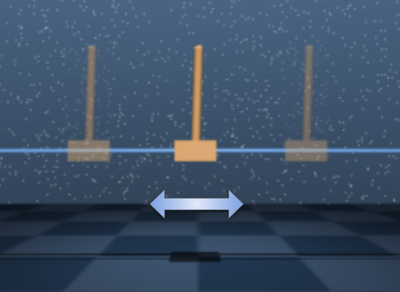
Figure 3: Depiction of translation symmetry of the cartpole environment in the Deepmind control suite (Tassa et al., 2020). The dynamics is invariant of the position along the horizontal bar, i.e. under shifts to the left and right symbolized by the arrow.

The cartpole’s dynamics admits a translation symmetry w.r.t. to its position i.e. it is invariant under left and right shifts, see fig.3. In the following we employ the KFC-algorithm for deriving symmetries from the Koopman latent representation in the cartpole gym environment (Brockman et al., 2016). Moreover, we highlight that this is possible when purposefully employing imprecise Koopman observables and operators. We choose the Koopman observables to simply be the state vector $g=s=(x,\dot{x},\theta,\dot{\theta})$; position, angle and their velocities. The dynamics is not linear in these observables, thus the latter constitute a rough approximation. Nevertheless we will see that our approach is successful. Note that symmetries can be inferred from the approximate Koopman space representation.

The trajectories are collected by a set of expert policies which admit the simple analytical form

$$\pi(s,z)=\Theta\big{(}0.015\,x\,+\,0.066\,\dot{x}\,+\,1.8\,\theta\,+\,0.32\,\dot{\theta}+z\big{)}\;,$$ (60)

where $\Theta$ is the Heaviside step function and $z\in\mathcal{U}(-0.2,0.2)$ a uniformly distributed random variable. The latter is sampled once at the beginning of each episode and is then fixed until the next one. This allows a for a wide variety of different expert policies from which we sample 100 trajectories each 1000 time-steps long. Note that Eq. (60) leads to an action set of $\{0,1\}$ as required by the cartpole gym environment (Brockman et al., 2016).

We empirically train a modified Koopman forward model Eq. (17) with trivial state embedding $g=s$ on the collected datasets and find that the approximate Koopman operator takes the form

$$\mathcal{K}\big{(}a=0\big{)}\;=\;\begin{pmatrix}1&0.02&-0.01&0.001\\ 0&1&0.6&0.8\\ 0&0&1&0.02\\ 0&-0.01&-0.7&-0.2\\ \end{pmatrix}$$ (61)

$$\mathcal{K}\big{(}a=1\big{)}\;=\;\begin{pmatrix}1&0.02&-0.009&0\\ 0&1&0.6&0.8\\ 0&0&1&0.02\\ 0&-0.009&-0.7&-0.2\\ \end{pmatrix}$$ (62)

for the actions $\{0,1\}$, respectively.

The translation symmetry generation matrix emerges when imposing it to be commuting with the Koopman operator taking the form

$$\sigma_{0}\;=\;\begin{pmatrix}-1&c_{1}&c_{2}&c_{3}\\ 0&0&0&0\\ 0&0&0&0\\ 0&0&0&0\\ \end{pmatrix}$$ (63)

where $c_{1}=-2.35,c_{2}=-25.95,c_{3}=-2$ for $a=0$ and $c_{1}=-2.60759,c_{2}=-29.0296,c_{3}=-2.22222$ for $a=1$.

The translation symmetry shift then takes the general form

$$\sigma_{a}^{\epsilon}=\mathds{1}+\epsilon\,\sigma_{0}=\left(\begin{array}[]{>{\columncolor{blue!20}}cccc}1-\epsilon&\epsilon\,c_{1}&\epsilon\,c_{2}&\epsilon\,c_{3}\\ &1&0&0\\ &0&1&0\\ &0&0&1\\ \end{array}\right)\,.$$ (64)

for $\epsilon\in\mathbb{R}$. Note that the Decoder and Encoder from and to Koopman space are simply the identify map in this case as we chose $g=s$. It is easy to see that Eq. (64) indeed is a translation symmetry. Note that the blue-shaded area guarantees that the position does not affect any of the other state variables. The latter, are mapped to themselves by the identity matrix in the lower right corner. Moreover, the red-shaded area implies that the initial position is mapped to another position by the symmetry map, controlled by the arbitrary $\epsilon$-parameter. We conclude that the translation symmetry operation emerges when imposing it to be commuting with the Koopman operator.

We show in theorem 3.9 that for $\epsilon\ll 1$ Eq. (64) is a local Lie symmetry. However, in this case we may show that the local symmetry can be extended to any global value. We take the matrix exponential of the generator $\sigma_{0}$ and find that it is equivalent to

$$\exp\big{(}\sigma_{0}\,t\big{)}=\hskip 91.04872pt$$

$$\left(\begin{array}[]{>{\columncolor{blue!20}}cccc}^{-t}&c_{1}\,(1-e^{-t})&c_{2}\,(1-e^{-t})&c_{3}\,(1-e^{-t})\\ &1&0&0\\ &0&1&0\\ &0&0&1\\ \end{array}\right),$$ (69)

for a parameter $t\in\mathbb{R}$. By comparison to Eq. (64) one infers that

$$\exp\big{(}\sigma_{0}\,t\big{)}=\sigma_{a}^{\epsilon}\;\;\;\text{if}\;\;\;\epsilon=1-e^{-t}\;\;.$$ (70)

In other words the composition of local symmetry transformations lead to extended "global" ones.

KFC++ algorithm: The translation symmetry can easily be inferred in a self supervised manner algorithmically by the KFC++ approach in Eq. (3.2) as

$${\bf\sigma^{\epsilon}_{a}\;\;:\;\;} \,s\mapsto\tilde{s}=\big{(}\mathds{1}+\sigma_{0}(\vec{\epsilon})\big{)}(s)\,,$$

$$\sigma_{0}(\vec{\epsilon}) ={\bf\mathscr{R}e}\big{(}\,U(a)\,\text{diag}(\epsilon_{1},\epsilon_{2},\epsilon_{3},\epsilon_{4})\,U^{-1}(a)\big{)}\;,\;\;\vspace{0.1 cm}$$

for $a=0,1$. One computes the eigenvalues $\lambda_{i},\,i=1,..,4$ and vectors $U(a=0,1)$ of the Koopman operators Eq. (61) and Eq. (62). Notable the systems admit an eigenvector $U_{0}=(1,0,0,0)$ to the eigenvalue $\lambda_{0}=1$. One infers that

$$\sigma^{\epsilon_{1}}_{a}=\mathds{1}+\sigma_{0}(\epsilon_{1},\epsilon_{2}=0,\epsilon_{3}=0,\epsilon_{4}=0)=$$

$$\left(\begin{array}[]{>{\columncolor{blue!20}}cccc}1+\epsilon_{1}&-\epsilon_{1}\,c_{1}&-\epsilon_{1}\,c_{2}&-\epsilon_{1}\,c_{3}\\ &1&0&0\\ &0&1&0\\ &0&0&1\\ \end{array}\right)\;\;.$$ (75)

Thus the translation symmetry is obtained by symmetry shifts w.r.t. the first eigenvalue. Moreover, we note that for the general setting i.e.  $\epsilon_{i}\neq 0,\,i=2,3,4$ one finds that the translation symmetry is naturally composed by other local symmetries as

$$\sigma^{\vec{\epsilon}}_{a}=\mathds{1}+\sigma_{0}(\vec{\epsilon})=\left(\begin{array}[]{>{\columncolor{blue!20}}cccc}1+\epsilon_{1}&\cdot&\cdot&\cdot\\ &\cdot&\cdot&\cdot\\ &\cdot&\cdot&\cdot\\ &\cdot&\cdot&\cdot\\ \end{array}\right)\;\;,$$ (80)

where we have used the symbol "$\cdot$" as proxy for in generally non-zero elements.

Local precision symmetry shifts Mujoco:

In this section we provide a quantitative analysis of the symmetry shifts generated by KFC++ in comparison to random shifts of the latent states. For the latter we choose the variance such that absolute state shift

$$\Delta S:=|\tilde{s}_{t}-s_{t}|+|\tilde{s}_{t+1}-s_{t+1}|$$ (81)

averaged over all sampled data points (D4RL) is comparable between the two setups. Moreover we simply use the encoder We then compare how well the shifted states are in alignment with the actual dynamic using the online Mujoco environment . To do so we set the environment state to the value $\tilde{s}_{t}$ and use the action $a_{t}$ to perform the environment step which we denote by $s_{t+1}=M(s_{t},a_{t})$ The performance metric is then given by

$$\Delta E:=|s_{t+1}-M(\tilde{s}_{t},a_{t})|\;\;.$$ (82)

Note that $\Delta E$ is simply the error to the actual dynamic of the environment. We take the model trained on the hopper-medium-expert dataset from section appendix D.1 to compute the symmetry shift. Moreover, for the comparison in Eq. (82) we split the state space into positions and velocities of the state vector, i.e. the first five elements of $s_{t+1}-M(\tilde{s}_{t},a_{t})$ give position while the remaining ones given velocities. The norm is taken subsequently. For the results see figure 4.

We conclude that there is a qualitative difference between the distributions obtained. Most notable the symmetry shift allows for a controlled shift by a larger $\Delta S$ while still maintaining a small error $\Delta E$. This amounts to a wide but accurate exploration of the environments state-space. Although we cannot say this conclusively we expect this to be the reason for the performance gains of KFC++ over random shifts.

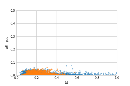
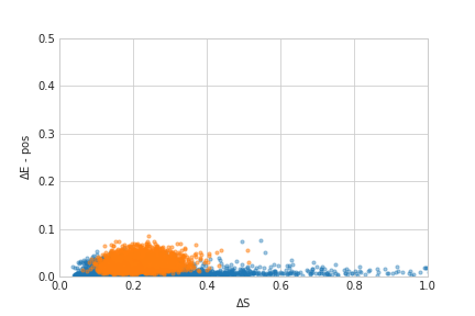
(a) Hopper position state shifts

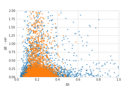
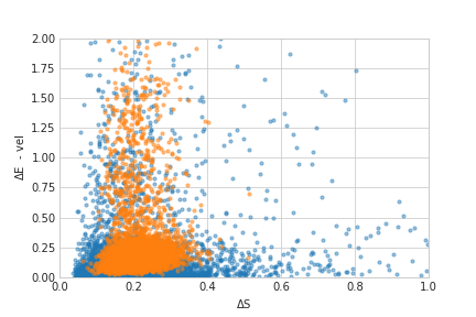
(b) Hopper velocity state shifts

Figure 4: Symmetry shifts vs. random latent space shifts of same magnitude in the mean of $\Delta S$ compared by its accuracy in the online evaluation in the gym Hopper-v3 environment. The first line shows the result where $s_{t}$ and $s_{t+1}$ are shifted by the same N-dimensional random variable. For the ablation study in line two we sample twice from the random variable for the shifts $s_{t}$ of $s_{t+1}$, respectively.

D.4 VAE without Koopman Operator

Task Name	S4RL-(Adv)	KFC	KFC++	VAE
Gym	61.61	66.36	67.76	52.90
Antmaze	62.88	65.52	67.35	54.26

Table 3: Results CQL with data-augmentation by a VAE with additive random latent space shifts. The results are averaged on the Gym and Antmaze tasks, respectively. We report the best results of the VAE over a hyperparameter search of the variance of the random variable.

We have performed an additional ablation study to compare KFC to a conventional VAE, see Table 3 for the results over the OpenAI Gym and Antmaze subset of the D4RL datasets. We find increased performance of KFC/KFC++ over data-augmentation by a common VAE with random latent space shifts. This ablation study is similar to the VAE baseline used in S4RL (Sinha et al., 2021), but the main difference is that we replace the Koopman operator in KFC with adding random noise in the learned latent representation of the VAE. We add noise of the form of $\mathcal{N}(0,\epsilon\times\mathcal{I})$; we perform a hyperparameter sweep over values for $\epsilon$ between $10^{-1}$ and $10^{-5}$. We report results with the best-performing noise value ($\epsilon=3\times 10^{-3}$). The VAE does not improve the performance over the S4RL baseline or KFC variants. We conclude that KFC/KFC++ is still the best-performing method due to the use of symmetry shifts and its Koopman latent representation, which is significantly better than adding random noise to the latent representation.

D.5 Prediction Model

As a further ablation study it is of interest to compare the symmetry induced state shifts tuple $(\tilde{s}_{t},\tilde{s}_{t+1})$ to one obtained by the forward prediction of our VAE-forward model Eq. (17).
KFC++prediction: In particular we use the forward prediction on $\tilde{s}_{t}$ obtained by the KFC++ shift, i.e.  $\tilde{s}_{t+1}=\mathcal{F}^{c=1}(\tilde{s}_{t},a_{t})$. We refer to this setup in the following as KFC++prediction. See table 4 for the results.
Fwd-prediction: Moreover, we study the case where we $\tilde{s}_{t}$ is obtained by a shift with a normally distributed random variable $\mathcal{N}(0,6\cdot 10^{-3})$ and then simply forward predict as $\tilde{s}_{t+1}=\mathcal{F}^{c=1}(\tilde{s}_{t},a_{t})$. This is comparable to conventional model based approaches employing our simple VAE forward model. This constitutes an ideal systematic comparison as the model, hyper-parameters and training procedure are identical to the one used in the KFC variants. Moreover, the variance of the random variable is such that the distance to the augmented states is comparable to the ones in KFC, see appendix D.2. See table 5 for the results.

Task Name	KFC	KFC++	KFC++-prediction
cheetah-random	48.6	49.2	46.5
cheetah-medium	55.9	59.1	53.7
cheetah-medium-replay	58.1	58.9	55.3
cheetah-medium-expert	79.9	79.8	76.3
hopper-random	10.4	10.7	10.8
hopper-medium	90.6	94.2	90.5
hopper-medium-replay	48.6	49.0	44.2
hopper-medium-expert	121.0	125.5	121.2
walker-random	19.1	17.6	15.6
walker-medium	102.1	108.0	105.3
walker-medium-replay	48.0	46.1	45.2
walker-medium-expert	114.0	115.6	114.5

Table 4: Results with prediction model KFC++-prediction on the Open AI Gym subset of the D4RL tasks. We report the mean normalized episodic rewards over 5 random seeds similar to the original D4RL paper (Fu et al., 2021).

Domain	Task Name	KFC	KFC++	Fwd-prediction
AntMaze	antmaze-umaze	96.9	99.8	92.7
	antmaze-umaze-diverse	91.2	91.1	90.1
	antmaze-medium-play	60.0	63.1	60.8
	antmaze-medium-diverse	87.1	90.5	88.0
	antmaze-large-play	24.8	25.6	23.1
	antmaze-large-diverse	33.1	34.0	29.3
Gym	cheetah-random	48.6	49.2	50
	cheetah-medium	55.9	59.1	50.1
	cheetah-medium-replay	58.1	58.9	56.4
	cheetah-medium-expert	79.9	79.8	71.3
	hopper-random	10.4	10.7	10.4
	hopper-medium	90.6	94.2	82.3
	hopper-medium-replay	48.6	49.0	40.8
	hopper-medium-expert	121.0	125.5	120.3
	walker-random	19.1	17.6	18.4
	walker-medium	102.1	108.0	103.2
	walker-medium-replay	48.0	46.1	41.7
	walker-medium-expert	114.0	115.3	111.8
Adroit	pen-human	61.3	60.0	49.4
	pen-cloned	71.3	68.4	50.2
	hammer-human	7.0	9.4	6.1
	hammer-cloned	3.0	4.2	4.2
	door-human	44.1	46.1	41.8
	door-cloned	3.6	5.6	1.2
	relocate-human	0.2	0.2	0.2
	relocate-cloned	-0.1	-0.1	-0.1
Franka	kitchen-complete	94.1	94.9	90.0
	kitchen-partial	92.3	95.9	84.6

Table 5: Results with prediction model Fwd-prediction on the D4RL tasks. We report the mean normalized episodic rewards over 5 random seeds similar to the original D4RL paper (Fu et al., 2021).

We conclude that KFC++prediction falls behind both KFC as well as KFC++. This was expected as the symmetry shift in the latter alters the original data points by means of the VAE which admits not only a much higher accuracy but also advanced generalisation capabilities to out of distribution values.
More interesting however is that Fwd-prediction falls behind both KFC as well as KFC++ as well as KFC++prediction. This is a strong indicator that the symmetry shifts provide superior out-of-distribution data for training a Q-learning algorithm.

D.6 Discussion

Although our KFC framework is suited best for the description of environments described by control dynamical systems the learned (in self-supervised manner) linear Koopman latent space representation may be applicable to a much wider set of tasks. However, there are notable shortcomings to the current implementation both conceptually as well as practically. The bilinearisation in Eq. (17) of the latent space theoretically assumes the dynamical system to be governed by Eq. (9), which is rather restrictive. Although a general non-affine control system admits a bilinearisation (Brunton et al., 2021) it generically requires the observables to depend on the action-space variables implicitly. Secondly, the Koopman operator formalism is theoretically defined by its action on an infinite dimensional observable space. The finite-dimensional approximation i.e. the latent space representation of the Koopman forward model in Eq. (17) lacks accuracy due to that. On the practical side our formalism requires data pre-processing which is computationally expensive, i.e. solving the Sylvester or eigenvalue problem for every data-point. Moreover, the Koopman forward model in Eq. (17) serves as a function approximation to two distinct tasks. Thus one faces a twofold accuracy vs. over-estimation problem which needs to be balanced. The systematic error in the VAE directly imprints itself on the state-data shift in Eqs. (16) and (3.2) and may thus conceal any potential benefit of the symmetry considerations. Lastly, the dynamical symmetries do not infer the reward. Thus the underlying working assumption is that the reward should not vary much in Eq. (16).

A note on the simplicity of the current algorithm:

Let us stress a crucial point. Algorithmically the symmetry maps are derived in two distinct ways KFC and KFC++. The latter, constitute a simple starting point to extract symmetries from our setup. More elaborate studies employing the extended literate on Koopman spectral analysis are desirable. Moreover, it is desirable to extend our framework to more complex latent space descriptions. It is our opinion that by doing so there is significant room for improvement both in the accuracy of the derived symmetry transformations as well their induced performance gains of Q-learning algorithms. Note that currently our VAE model is of very simple nature and the symmetries are extracted in a rather uneducated way. While the Sylvester algorithm simply converges to one out of many symmetry transformations for the KFC++ algorithm we omit all the information of the imaginary part, let alone utilize concrete spectral information.

References

- (1) Sylvester algorithm - scipy.org. URL https://docs.scipy.org/doc/scipy-0.15.1/reference/generated/scipy.linalg.solve_sylvester.html.
- Agarwal et al. (2020) Agarwal, R., Schuurmans, D., and Norouzi, M. An optimistic perspective on offline reinforcement learning. In International Conference on Machine Learning, 2020.
- Balaraman & Andrew (2004) Balaraman, R. and Andrew, G. B. Approximate homomorphisms: A framework for non-exact minimization in Markov decision processes. In In International Conference on Knowledge Based Computer Systems, 2004.
- Brockman et al. (2016) Brockman, G., Cheung, V., Pettersson, L., Schneider, J., Schulman, J., Tang, J., and Zaremba, W. Openai gym. arXiv: 1606.01540, 2016.
- Brunton et al. (2021) Brunton, S. L., Budišić, M., Kaiser, E., and Kutz, J. N. Modern Koopman theory for dynamical systems. arXiv: 2102.12086, 2021.
- Caselles-Dupré et al. (2019) Caselles-Dupré, H., Garcia Ortiz, M., and Filliat, D. Symmetry-based disentangled representation learning requires interaction with environments. In Wallach, H., Larochelle, H., Beygelzimer, A., d'Alché-Buc, F., Fox, E., and Garnett, R. (eds.), Advances in Neural Information Processing Systems, volume 32. Curran Associates, Inc., 2019.
- Ernst et al. (2005) Ernst, D., Geurts, P., and Wehenkel, L. Tree-based batch mode reinforcement learning. Journal of Machine Learning Research, 6(18):503–556, 2005.
- Fu et al. (2021) Fu, J., Kumar, A., Nachum, O., Tucker, G., and Levine, S. D4rl: Datasets for deep data-driven reinforcement learning. arXiv: 2004.07219, 2021.
- Fujimoto et al. (2019) Fujimoto, S., Meger, D., and Precup, D. Off-policy deep reinforcement learning without exploration. In Proceedings of the 36th International Conference on Machine Learning, volume 97 of Proceedings of Machine Learning Research, pp. 2052–2062. PMLR, 09–15 Jun 2019.
- Gelada et al. (2019) Gelada, C., Kumar, S., Buckman, J., Nachum, O., and Bellemare, M. G. DeepMDP: Learning continuous latent space models for representation learning. In Chaudhuri, K. and Salakhutdinov, R. (eds.), Proceedings of the 36th International Conference on Machine Learning, volume 97 of Proceedings of Machine Learning Research, pp. 2170–2179. PMLR, 09–15 Jun 2019. URL https://proceedings.mlr.press/v97/gelada19a.html.
- Goswami & Paley (2017) Goswami, D. and Paley, D. A. Global bilinearization and controllability of control-affine nonlinear systems: A Koopman spectral approach. 2017 IEEE 56th Annual Conference on Decision and Control (CDC), pp. 6107–6112, 2017.
- Ha & Schmidhuber (2018) Ha, D. and Schmidhuber, J. Recurrent world models facilitate policy evolution. In Bengio, S., Wallach, H., Larochelle, H., Grauman, K., Cesa-Bianchi, N., and Garnett, R. (eds.), Advances in Neural Information Processing Systems, volume 31. Curran Associates, Inc., 2018. URL https://proceedings.neurips.cc/paper/2018/file/2de5d16682c3c35007e4e92982f1a2ba-Paper.pdf.
- Haarnoja et al. (2017) Haarnoja, T., Tang, H., Abbeel, P., and Levine, S. Reinforcement learning with deep energy-based policies. In Precup, D. and Teh, Y. W. (eds.), Proceedings of the 34th International Conference on Machine Learning, volume 70 of Proceedings of Machine Learning Research, pp. 1352–1361. PMLR, 06–11 Aug 2017.
- Haarnoja et al. (2018) Haarnoja, T., Zhou, A., Abbeel, P., and Levine, S. Soft actor-critic: Off-policy maximum entropy deep reinforcement learning with a stochastic actor. In Dy, J. and Krause, A. (eds.), Proceedings of the 35th International Conference on Machine Learning, volume 80 of Proceedings of Machine Learning Research, pp. 1861–1870. PMLR, 10–15 Jul 2018.
- Higgins et al. (2018) Higgins, I., Amos, D., Pfau, D., Racaniere, S., Matthey, L., Rezende, D., and Lerchner, A. Towards a definition of disentangled representations. arXiv: 1812.02230, 2018.
- Iwata & Kawahara (2021) Iwata, T. and Kawahara, Y. Controlling nonlinear dynamical systems with linear quadratic regulator-based policy networks in Koopman space. In Proc. of the 60th IEEE Conf. on Decision and Control (CDC’21), pp. 5086–5091, 2021.
- Kaiser et al. (2021) Kaiser, E., Kutz, J. N., and Brunton, S. L. Data-driven discovery of Koopman eigenfunctions for control. Machine Learning: Science and Technology, 2:035023, 2021.
- Kalashnikov et al. (2018) Kalashnikov, D., Irpan, A., Pastor, P., Ibarz, J., Herzog, A., Jang, E., Quillen, D., Holly, E., Kalakrishnan, M., Vanhoucke, V., and Levine, S. Scalable deep reinforcement learning for vision-based robotic manipulation. In Billard, A., Dragan, A., Peters, J., and Morimoto, J. (eds.), Proceedings of The 2nd Conference on Robot Learning, volume 87 of Proceedings of Machine Learning Research, pp. 651–673. PMLR, 29–31 Oct 2018.
- Kingma & Welling (2013) Kingma, D. P. and Welling, M. Auto-encoding variational Bayes. arXiv: 1312.6114, 2013.
- Koopman (1931) Koopman, B. O. Hamiltonian systems and transformation in Hilbert space. Proceedings of the National Academy of Sciences of the United States of America, 17(5):315–318, 1931.
- Kumar et al. (2020) Kumar, A., Zhou, A., Tucker, G., and Levine, S. Conservative Q-learning for offline reinforcement learning. In Larochelle, H., Ranzato, M., Hadsell, R., Balcan, M. F., and Lin, H. (eds.), Advances in Neural Information Processing Systems, volume 33, pp. 1179–1191. Curran Associates, Inc., 2020.
- Laskin et al. (2020a) Laskin, M., Lee, K., Stooke, A., Pinto, L., Abbeel, P., and Srinivas, A. Reinforcement learning with augmented data. In Larochelle, H., Ranzato, M., Hadsell, R., Balcan, M. F., and Lin, H. (eds.), Advances in Neural Information Processing Systems, volume 33, pp. 19884–19895. Curran Associates, Inc., 2020a.
- Laskin et al. (2020b) Laskin, M., Srinivas, A., and Abbeel, P. CURL: Contrastive unsupervised representations for reinforcement learning. In III, H. D. and Singh, A. (eds.), Proceedings of the 37th International Conference on Machine Learning, volume 119 of Proceedings of Machine Learning Research, pp. 5639–5650. PMLR, 13–18 Jul 2020b.
- Li et al. (2010) Li, L., Chu, W., Langford, J., and Schapire, R. E. A contextual-bandit approach to personalized news article recommendation. In Proceedings of the 19th international conference on World wide web, pp. 661–670, 2010.
- Li et al. (2020) Li, Y., He, H., Wu, J., Katabi, D., and Torralba, A. Learning compositional Koopman operators for model-based control. In Proc. of the 8th Int’l Conf. on Learning Representation (ICLR’20), 2020.
- Mauroy et al. (2020) Mauroy, A., Mezić, I., and Susuki, Y. The Koopman Operator in Systems and Control: Concepts, Methodologies, and Applications. Springer, 2020.
- Mezić (2005) Mezić, I. Spectral properties of dynamical systems, model reduction and decompositions. Nonlinear Dynamics, 41:309–325, 2005.
- Morton et al. (2019) Morton, J., Witherden, F. D., and Kochenderfer, M. J. Deep variational Koopman models: Inferring Koopman observations for uncertainty-aware dynamics modeling and control. In Proceedings of the 28th International Joint Conference on Artificial Intelligence, IJCAI’19. AAAI Press, 2019.
- Nair & Hinton (2010) Nair, V. and Hinton, G. E. Rectified linear units improve restricted Boltzmann machines. In Icml, 2010.
- Ohnishi et al. (2021) Ohnishi, M., Ishikawa, I., Lowrey, K., Ikeda, M., Kakade, S., and Kawahara, Y. Koopman spectrum nonlinear regulator and provably efficient online learning. arXiv: 2106.15775, 2021.
- Paszke et al. (2019) Paszke, A., Gross, S., Massa, F., Lerer, A., Bradbury, J., Chanan, G., Killeen, T., Lin, Z., Gimelshein, N., Antiga, L., et al. Pytorch: An imperative style, high-performance deep learning library. Advances in neural information processing systems, 32:8026–8037, 2019.
- Rajeswaran et al. (2017) Rajeswaran, A., Kumar, V., Gupta, A., Vezzani, G., Schulman, J., Todorov, E., and Levine, S. Learning complex dexterous manipulation with deep reinforcement learning and demonstrations. arXiv: 1709.10087, 2017.
- Salova et al. (2019) Salova, A., Emenheiser, J., Rupe, A., Crutchfield, J. P., and D’Souza, R. M. Koopman operator and its approximations for systems with symmetries. Chaos: An Interdisciplinary Journal of Nonlinear Science, 29(9):093128, 2019. doi: 10.1063/1.5099091.
- Sinha et al. (2020) Sinha, S., Nandanoori, S. P., and Yeung, E. Koopman operator methods for global phase space exploration of equivariant dynamical systems. arXiv: 2003.04870, 2020.
- Sinha et al. (2021) Sinha, S., Mandlekar, A., and Garg, A. S4RL: Surprisingly Simple Self-Supervision for Offline Reinforcement Learning. In Conference on Robot Learning, 2021.
- Tassa et al. (2020) Tassa, Y., Tunyasuvunakool, S., Muldal, A., Doron, Y., Liu, S., Bohez, S., Merel, J., Erez, T., Lillicrap, T., and Heess, N. dm control: Software and tasks for continuous control. arXiv: 2006.12983, 2020.
- van der Pol et al. (2020) van der Pol, E., Worrall, D., van Hoof, H., Oliehoek, F., and Welling, M. Mdp homomorphic networks: Group symmetries in reinforcement learning. In Larochelle, H., Ranzato, M., Hadsell, R., Balcan, M. F., and Lin, H. (eds.), Advances in Neural Information Processing Systems, volume 33, pp. 4199–4210. Curran Associates, Inc., 2020.
- Wu et al. (2019) Wu, Y., Tucker, G., and Nachum, O. Behavior regularized offline reinforcement learning. arXiv: 1911.11361, 2019.
- Yu et al. (2019) Yu, T., Quillen, D., He, Z., Julian, R., Hausman, K., Finn, C., and Levine, S. Meta-world: A benchmark and evaluation for multi-task and meta reinforcement learning. arXiv: 1910.10897, 2019.
- Zhang et al. (2021) Zhang, A., McAllister, R. T., Calandra, R., Gal, Y., and Levine, S. Learning invariant representations for reinforcement learning without reconstruction. In International Conference on Learning Representations, 2021. URL https://openreview.net/forum?id=-2FCwDKRREu.
- Zhu et al. (2020) Zhu, Y., Wong, J., Mandlekar, A., and Martín-Martín, R. robosuite: A modular simulation framework and benchmark for robot learning. arXiv: 2009.12293, 2020.