Primordial black holes and scalar induced gravitational waves from Higgs inflation with noncanonical kinetic term

Abstract

We resolve the potential-restriction problem in K/G inflation by introducing nonminimal coupling. In this context, Higgs field successfully drives inflation satisfying CMB observations while enhancing curvature perturbations at small scales, which in turn accounts for primordial black holes (PBHs) and scalar induced gravitational waves (SIGWs). We then uncover the effect of the non-canonical kinetic coupling function in more detail and study its the observational constraint. Besides, we also give the gauge invariant expression for the integral kernel of SIGWs, which is related to terms propagating with the speed of light. Finally, the non-Gaussian effect on PBH abundance and SIGWs is studied. We find that non-Gaussianity makes PBHs form more easily, but its effect on the energy density of SIGWs is negligible.

I Introduction

The overdense inhomogeneities in the radiation era could gravitationally collapse to form primordial black holes (PBHs) Carr and Hawking (1974); Hawking (1971), which could be used to account for Dark Matters (DM) Ivanov et al. (1994); Frampton et al. (2010); Belotsky et al. (2014); Khlopov et al. (2005); Clesse and García-Bellido (2015); Carr et al. (2016); Inomata et al. (2017a); García-Bellido (2017); Kovetz (2017). Due to the vast range of masses, PBHs may explain the Black Hole binaries with tiny effective spin detected by LIGO-Virgo Collaboration Abbott et al. (2016a, b); Bird et al. (2016); Sasaki et al. (2016). These density inhomogeneities can be generated from the inflationary stage, and cause collapse to form PBHs after horizon reentry. This mechanism requires the amplitude of the primordial curvature perturbation to be $A_{s}\sim\mathcal{O}(10^{-2})$ Sato-Polito et al. (2019) while the amplitude has been constrained by the cosmic microwave background (CMB) anisotropy measurements to be $A_{s}\approx 2.1\times 10^{-9}$ at the pivot scale $k_{*}=0.05\ \text{Mpc}^{-1}$ Akrami et al. (2020). Thus the enhancement of the amplitude can occur exclusively at small scales.

A way to enhance the curvature perturbation is to provide a dramatic decrease in the velocity of the inflaton, and thus the slow-roll condition is violated. This can be achieved by an inflationary potential with an inflection point Germani and Prokopec (2017); Motohashi and Hu (2017); Di and Gong (2018); Wu et al. (2021) or a step-like feature Inomata et al. (2021a). For other enhancement mechanisms, please see Refs. Fu et al. (2019); Kawai and Kim (2021); Chen et al. (2021); Teimoori et al. (2021); Liu and Xu (2021); Zheng et al. (2021); Heydari and Karami (2021a, b); Cai et al. (2021a); Wang et al. (2021); Ahmed et al. (2021). While the inflection point does lead to the decrease in $\dot{\phi}$, and thus the enhancement of the power spectrum, it is a challenge to fine-tune the model parameters to enhance the power spectrum to the order of $\mathcal{O}(10^{-2})$ with the total number of $e$-folds within $N\simeq 50\text{-}60$ Sasaki et al. (2018); Passaglia et al. (2019). Meanwhile, a new mechanism with a peak function $G(\phi)$ in the noncanonical kinetic term was proposed to enhance the primordial power spectrum at small scales Lin et al. (2020); Yi et al. (2021a, b); Gao et al. (2021); Yi and Zhu (2021); Zhang et al. (2021a, b); Solbi and Karami (2021). As we will show in our paper, the peak function serves not only the enhancement of the curvature perturbation, but also the fast exit of inflation keeping the $e$-folds within $N\simeq 50\text{-}60$. Both sharp and broad peak functions are acceptable Yi et al. (2021b), which contribute up to $\sim 20$ $e$-folds so that the usual slow-roll inflation epoch should be kept $30\text{-}40$ $e$-folds and the inflationary potential may be restricted. To cure this problem, this mechanism was improved by generalizing the noncanonical kinetic term to $G(\phi)+f(\phi)$ Yi et al. (2021a, b); Gao et al. (2021); Yi and Zhu (2021). In this paper, we will show another way to avoid this potential-restriction problem by employing the nonminimal coupling between gravity and scalar field.

On the other hand, as the only scalar field verified so far, Higgs, if drives inflation, suffers from the problem of unacceptably large tensor-to-scalar ratio $r$. To satisfy CMB observation, nonminimal (derivative) couplings $\xi\phi^{2}R$, $G^{\mu\nu}\partial_{\mu}\phi\partial_{\nu}\phi$ are introduced to reduce $r$ Kaiser (1995); Bezrukov and Shaposhnikov (2008); Germani and Kehagias (2010); Germani et al. (2014); Hamada et al. (2014); Yang et al. (2016); Fumagalli et al. (2018, 2020). Taking into account the running of self-coupling constant and the nonminimal coupling between Higgs field and gravity, the effective potential in Einstein frame possesses an inflection point, which can enhance the curvature perturbation. However, such an enhancement is only of five orders of magnitude compared with CMB constraint $A_{s}\sim\mathcal{O}(10^{-9})$, and is unable to produce a significant abundance of PBHs Ezquiaga et al. (2018); Bezrukov et al. (2018). In our paper, we will show that, by introducing a noncanonical kinetic term and a nonminimal coupling, the Higgs-field-driving inflation is compatible with CMB observation while simultaneously enhancing the curvature perturbations to order $\mathcal{O}(10^{-2})$ at small scales.

The production of PBHs by the enhanced primordial curvature perturbation is accompanied by the generation of scalar induced gravitational waves (SIGWs) Matarrese et al. (1998); Mollerach et al. (2004); Ananda et al. (2007); Baumann et al. (2007); Garcia-Bellido et al. (2017); Saito and Yokoyama (2009, 2010); Bugaev and Klimai (2010, 2011); Alabidi et al. (2012); Orlofsky et al. (2017); Nakama et al. (2017); Inomata et al. (2017b); Cheng et al. (2018); Kawai and Kim (2021); Cai et al. (2019a, 2020, b), for recent review, please refer Domènech (2021), which consist of the stochastic background and can be tested by Pulsar Timing Arrays (PTA) Ferdman et al. (2010); Hobbs et al. (2010); McLaughlin (2013); Hobbs (2013) and the space based GW observatories like Laser Interferometer Space Antenna (LISA) Amaro-Seoane et al. (2017), Taiji Hu and Wu (2017) and TianQin Luo et al. (2016). Therefore, the observations of both PBHs and SIGWs can be used to constrain the amplitude enhancement of the primordial curvature perturbation during inflation and thus to probe the physics in the early universe.

The paper is organized as follows. In Sec. II, we show our mechanism to enhance the curvature perturbation with Higgs potential by combining the noncanonical kinetic term with the nonminimal coupling. The PBH abundance and the energy density of SIGWs generated by Higgs inflation are presented in Sec. III. In Sec.IV, we discuss the effect of the non-Gaussianity on PBH abundance and SIGWs. We conclude the paper in Sec.V.

II K/G inflation with nonminimal coupling

II.1 Review of K/G inflation

An idea to enhance curvature perturbation is to temporarily change the friction term in curvature perturbation equation

$$\zeta^{\prime\prime}_{k}+2\frac{z^{\prime}}{z}\zeta^{\prime}_{k}+k^{2}\zeta_{k}=0,$$ (1)

into a driving term during inflation. To wit, $z^{\prime}/z<0$. For K/G inflation Lin et al. (2020) with the noncanonical kinetic term $[1+G(\phi)]X$ where $X=\dot{\phi}^{2}/2$, the friction term is

$$\frac{z^{\prime}}{z}=aH\left[1+\epsilon_{1}-\epsilon_{2}+\frac{G_{\phi}\dot{\phi}}{2H(1+G)}\right],$$ (2)

where $\epsilon_{1}=-\dot{H}/H^{2},\epsilon_{2}=-\ddot{\phi}/(H\dot{\phi})$ are slow-roll parameters. To make $z^{\prime}/z<0$, we could temporarily keep the second slow-roll parameter $\epsilon_{2}>0$ and large, i.e. the velocity of scalar field should dramatically decrease. The scalar field equation is

$$H\dot{\phi}(3-\epsilon_{2})+V_{\phi}^{\text{eff}}=0,$$ (3)

where

$$V^{\text{eff}}_{\phi}=\frac{V_{\phi}+XG_{\phi}}{1+G}$$ (4)

is the gradient of effective potential and the subscript $\phi$ represents the derivative with respect to $\phi$. In our orignal paper Lin et al. (2020), we have shown that the power spectrum can be enhanced if $G$ has a peak. Motivated by Brans-Dicke theory Brans and Dicke (1961) with coupling $1/\phi^{q}$, we choose Lin et al. (2020); Yi et al. (2021b)

$$G(\phi)=\frac{h}{1+(\left|\phi-\phi_{c}\right|/c)^{q}},$$ (5)

where $h,c$ determine the amplitude and width of the peak, respectively. $q$ controls the shape of the enhanced power spectrum. Larger $q$ may give a broad peak in the power spectrum. The peak position $\phi_{c}$ is related to the peak mass of PBH and the peak frequency of SIGWs. Away from the peak, $G\approx 0$ such that the usual slow-roll inflation is recovered., In fact, by performing a field-redefinition $d\varphi=\sqrt{1+G(\phi)}d\phi$, K/G inflation is equivalent to a class of the canonical inflation with the potential $U(\varphi)$ possessing an inflection point, as shown in Fig.1.

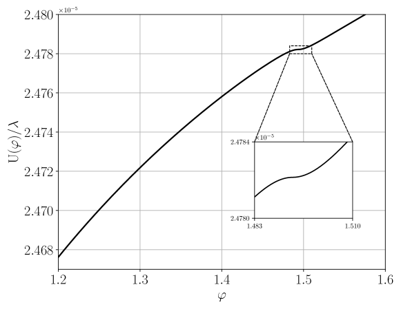
Figure 1: After the field redefinition, the corresponding canonical potential possesses an inflection point.

II.2 Potential-restriction problem and K/G inflation with nonminimal coupling

Note that due to the dramatic decrease in $\dot{\phi}$, the peak function $G(\phi)$ will contribute up to $\sim 20$ $e$-folds, and the usual slow-roll inflation epoch should be kept e-folds $N\simeq 30\text{-}40$ so that the total $e$-folds during inflation is within $N\simeq 50\text{-}60$. Thus the usual K/G inflation suffers from the potential-restriction problem. For power-law potential $V=\lambda\phi^{p}$ with $0<p\leq 4$, the $e$-folds during slow-roll inflation can be expressed in terms of the spectrum index as $N_{sr}\approx(p+2)/2(1-n_{s})$. To keep $N_{sr}\simeq 30\text{-}40$, the power-law index $p$ should be bounded by $p\lesssim 1$. Thus this mechanism does not work for Higgs field ($p=4$). Besides, the tensor-to-scalar ratio predicted by inflation with Higgs potential is

$$r\approx 8\left(\frac{V_{\phi}}{V}\right)^{2}=\frac{8p(1-n_{s})}{p+2}\Big{|}_{p=4}\approx 0.18,$$ (6)

which is incompatible with observational constraints $r_{0.05}<0.036(95\%\rm{CL})$ Ade et al. (2021).

To realize the enhanced power spectrum with Higgs field, we combine K/G enhancement mechanism with the nonmiminal coupling between Higgs field and gravity, i.e. $\Omega(\phi)\tilde{R}$ . The action in Jordan frame is

$$S=\int d^{4}x\sqrt{-\tilde{g}}\left[\frac{1}{2}\Omega(\phi)\tilde{R}(\tilde{g})-\frac{1}{2}\omega(\phi)\tilde{g}^{\mu\nu}\nabla_{\mu}\phi\nabla_{\nu}\phi-V(\phi)\right].$$ (7)

Under conformal transformation $g_{\mu\nu}=\Omega(\phi)\tilde{g}_{\mu\nu}$, the action in Einstein frame becomes

$$S=\int d^{4}x\sqrt{-g}\left[\frac{1}{2}R(g)-\frac{1}{2}W(\phi)g^{\mu\nu}\nabla_{\mu}\phi\nabla_{\nu}\phi-U(\phi)\right],$$ (8)

where

$$W(\phi)=\frac{3}{2}\frac{(d\Omega/d\phi)^{2}}{\Omega^{2}(\phi)}+\frac{\omega(\phi)}{\Omega(\phi)},\quad U(\phi)=V(\phi)/\Omega^{2}(\phi).$$ (9)

For power-law potential $V(\phi)=\lambda\phi^{p}$, we choose the conformal factor

$$\Omega(\phi)=1+\xi\phi^{p/2}.$$ (10)

The conformal factor can flatten the power-law potential so that the tensor-to-scalar ratio is within the CMB observation and the $e$-folds of usual slow-roll inflation is kept within $30\text{-}40$. By choosing the appropriate coupling function $\omega(\phi)$ in Jordan frame, the coupling function in Einstein frame becomes

$$W(\phi)=1+G(\phi).$$ (11)

Models	$\phi_{*}$	$\phi_{c}$	$\lambda$	$h$	$c$	$N$	$n_{s}$	$r$	$k_{\text{peak}}/\text{Mpc}^{-1}$	$\mathcal{P}_{\zeta(\text{peak})}$
H1	1.6	1.515	$2.3\times 10^{-7}$	$8\times 10^{7}$	$8.3\times 10^{-11}$	63	0.97	0.0007	$2.84\times 10^{5}$	0.036
H2	1.6	1.3	$2.3\times 10^{-7}$	$8.15\times 10^{7}$	$1.309\times 10^{-10}$	63	0.966	0.0007	$4\times 10^{12}$	0.0258
WH	1.6	1.47	$2.3\times 10^{-7}$	$8\times 10^{7}$	$7.445\times 10^{-10}$	64	0.965	0.0007	$2.99\times 10^{5}$	0.016
Q	1.3	0.98	$3.3\times 10^{-7}$	$1.5\times 10^{7}$	$9.35\times 10^{-10}$	64	0.965	0.0007	$6.53\times 10^{12}$	0.013

Table 1: The chosen parameters and the results for the scalar power spectrum at small peak scales.

We will show now this mechanism works for generic power-law potentials. To be specific, we will numerically calculate the power spectrum for Higgs field ($p=4$) and power-law potential with $p=2$. We use labels ”H” and ”WH” to represent Higgs inflations with the shape parameter $q=1$ and $q=6/5$, respectively and use label ”Q” to represent power-law inflation with $p=2$. The self-coupling constant $\lambda$ is set as $\mathcal{O}(10^{-7})$ to satisfy the amplitude of power spectrum $A_{s}\simeq 2\times 10^{-9}$ at CMB scale. To get $\mathcal{O}(10^{-2})$ enhancement at small scale, we choose $h\sim\mathcal{O}(10^{7})$. The nonminimal coupling constant is taken as $\xi=100$. With the model parameters listed in Table 1, solving the equations for the background and the perturbations numerically, the results for the scalar power spectrum are shown in Table 1 and Fig.2. From these results, we can see that $n_{s}$ and $r$ are well within the CMB observation constraints, $n_{s}=0.9649\pm 0.0042(68\%\rm{CL})$ and $r_{0.05}<0.036(95\%\rm{CL})$ Akrami et al. (2020); Ade et al. (2021). In particular, due to conformal factor, $r$ can be reduced to order $\mathcal{O}(10^{-4})$. The total $e$-folds are around $60$. The power spectrum is enhanced to $\mathcal{O}(10^{-2})$ at the scales $\mathcal{O}(10^{5})~{}\rm{Mpc}^{-1}$ and $\mathcal{O}(10^{12})~{}\rm{Mpc}^{-1}$. To be specific, the power spectrum for models H1 and WH are enhanced at the scale $\mathcal{O}(10^{5})~{}\rm{Mpc}^{-1}$ and the power spectrum for models H2 and Q are enhanced at the scale $\mathcal{O}(10^{12})~{}\rm{Mpc}^{-1}$. In addition, the shape parameter $q=1$ produces a sharp peak while the larger shape parameter $q=6/5$ produces the broad peak.

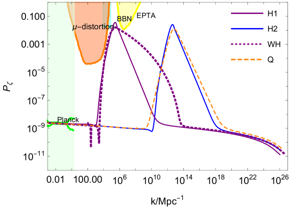
Figure 2: The results for the scalar power spectrum for Model H1 (the purple line), Model H2 (the blue line), Model WH (the dotted purple line) and Model Q (the orange dashed line). The green lines show the scale-dependent behavior of the power spectrum. The light-green shaded region is excluded by the CMB observations Akrami et al. (2020). The light-grey, light-blue and thistle regions show the constraints from $\mu$-distortion of CMB Fixsen et al. (1996), the effect on the ratio between neutron and proton during the big bang nucleosynthesis (BBN) Inomata et al. (2016) and the PTA observations Inomata and Nakama (2019), respectively.

II.3 Non-canonical kinetic coupling function and its observational constraint

In this subsection, we will uncover the effect of non-canonical kinetic coupling function in more detail and study the observational constraint on the parameter space of non-canonical kinetic coupling function.

In Fig.3, we show the numerical results for the behaviors of the gradient of effective potential $V^{\text{eff}}_{\phi}$ and the second slow-roll parameter $\epsilon_{2}$ around the peak $\phi_{c}=1.515$ for Model H1. As we can see, as $\phi$ rolls down to the right region of the peak where $G_{\phi}$ is negative and very large, the gradient of effective potential satisfies $V^{\text{eff}}_{\phi}<0$ so that $\epsilon_{2}>3$ and $\dot{\phi}$ will dramatically decrease, and thus enhance curvature perturbation. As $\phi$ leaves for the left region where $G_{\phi}$ is positive and very large, the gradient of effective potential $V^{\text{eff}}_{\phi}>0$ such that $\epsilon_{2}<0$. Here $\dot{\phi}$ will violently increase and help inflation exit. To sum up, phenomenologically, the peak function $G$ enables not only the dramatic decrease in $\dot{\phi}$, which further leads to the enhancement of the curvature perturbation but also the fast exit of inflation.

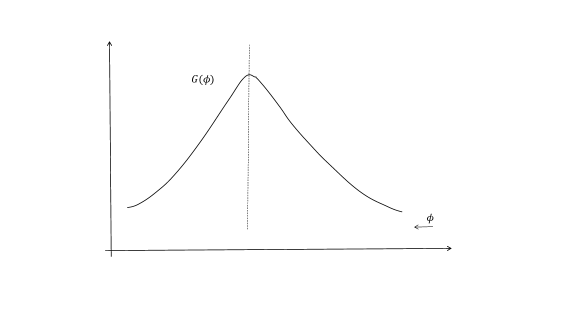
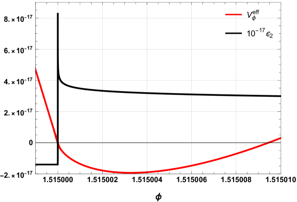
Figure 3: The peak function $G(\phi)$ and numerical results for the behaviors of $V^{\text{eff}}_{\phi}$ and $\epsilon_{2}$ around the peak $\phi_{c}=1.515$ for Model H1.

$c$	$8.3\times 10^{-11}$	$8.8\times 10^{-11}$	$9.3\times 10^{-11}$	$1\times 10^{-10}$	$2\times 10^{-10}$
Upper bound on $h$	$8.05\times 10^{7}$	$7.6\times 10^{7}$	$7.2\times 10^{7}$	$6.7\times 10^{7}$	$3.4\times 10^{7}$

Table 2: Constraint on K/G model with with Higgs potantial from LIGO merger rate. Here $\phi_{c}=1.515$ and $q=1$.

$c$	$1.4\times 10^{-10}$	$2\times 10^{-10}$	$2.5\times 10^{-10}$	$3\times 10^{-10}$	$3.2\times 10^{-10}$
Upper bound on $h$	$8\times 10^{7}$	$5.65\times 10^{7}$	$4.55\times 10^{7}$	$3.85\times 10^{7}$	$3.7\times 10^{7}$

Table 3: Constraint on K/G model with with Higgs potential from White Dwarf Explosion. Here $\phi_{c}=1.28$ and $q=1$.

The observational constraints on the present PBH abundance can be used to to constrain the power spectrum for primordial curvature perturbations at small scales and thus the range of parameter space of non-canonical kinetic coupling function. Now let us study the observation constraints on K/G model with Higgs potential in detail. The LIGO merger rates Ali-Haïmoud et al. (2017) constrain the power spectrum as $\mathcal{P}_{\zeta}\lesssim 0.04$ for $8.9\times 10^{4}~{}\text{Mpc}^{-1}\lesssim k\lesssim 4.9\times 10^{5}~{}\text{Mpc}^{-1}$ Sato-Polito et al. (2019). This $k$-range of this constraint can be used to bound the amplitude parameter $h$ of our models with the peak position $1.5\lesssim\phi_{c}$ for the shape factor $q=1$ and $1.47\lesssim\phi_{c}$ for $q=6/5$, which could further apply to the realizations of Models H1 and WH. To be specific, by choosing the peak position $\phi_{c}=1.515$ and $q=1$ and varying the width parameter $c$, we numerically find the upper bound on the amplitude parameter $h$ and the results are shown in Tab.2. The larger the parameter $c$ is, the lower the upper bound on $h$ will be. This result is well comprehensive. For a wider peak function, the velocity of the inflaton decreases more dramatically. Therefore a smaller amplitude parameter $h$ is required to realize the same enhancement on the curvature perturbation. Moreover, the White Dwarf Explosion Graham et al. (2015) constrains the power spectrum to be $\mathcal{P}_{\zeta}\lesssim 0.023$ for $5.1\times 10^{12}\text{Mpc}^{-1}\lesssim k\lesssim 2\times 10^{13}\text{Mpc}^{-1}$. This $k$-range of this constraint can be used to bound the amplitude parameter $h$ of our models with the peak position $1.27\lesssim\phi_{c}$ for $q=1$, which could further apply to the realizations of Models H2. The corresponding bound on $h$ is shown in Tab.3 and here we choose $\phi_{c}=1.28$ and $q=1$.

III Primordial black holes and scalar induced gravitational waves

The large curvature perturbation from inflation can induce PBHs and GWs at radiation era. In this section, we will calculate PBHs abundance and SIGWs from K/G inflation with nonminimal coupling. Before that, we will first consider the gauge issue on SIGWs and give a gauge invariant expression for the integral kernel of SIGWs.

III.1 The gauge invariant expression for the integral kernel of SIGWs

Considering a metric perturbation

$$\mathrm{d}s^{2}=a^{2}\left[-(1+2\phi)\mathrm{d}\tau^{2}+2B_{,i}\mathrm{~{}d}x^{i}\mathrm{~{}d}\tau+\left((1-2\psi)\delta_{ij}+2E_{,ij}+\frac{1}{2}h_{ij}^{\mathrm{TT}}\right)\mathrm{d}x^{i}\mathrm{~{}d}x^{j}\right],$$ (12)

the scalar-induced tensor perturbations $h^{\text{TT}}_{ij}$ satisfy Ananda et al. (2007); Baumann et al. (2007)

$$h_{ij}^{\mathrm{TT}\prime\prime}+2\mathcal{H}h_{ij}^{\mathrm{TT}\prime}-\nabla^{2}h_{ij}^{\mathrm{TT}}=4\mathcal{T}_{ij}^{lm}s_{lm},$$ (13)

where $\mathcal{H}=aH$, $\mathcal{T}_{ij}^{lm}$ is the projection tensor extracting the transverse and traceless part of a tensor and the scalar source is Lu et al. (2020)

$$\begin{split}-s_{ij}=&\psi_{,i}\psi_{,j}+\phi_{,i}\phi_{,j}-\sigma_{,ij}\left(\phi^{\prime}+\psi^{\prime}-\nabla^{2}\sigma\right)+\left(\psi_{,i}^{\prime}\sigma_{,j}+\psi_{,j}^{\prime}\sigma_{,i}\right)-\sigma_{,ik}\sigma_{,jk}+2\psi_{,ij}\left(\phi+\psi\right)\\ &-8\pi Ga^{2}({\rho_{0}}+{P_{0}})\delta V_{,i}\delta V_{,j}-2\psi_{,ij}\nabla^{2}E+2E_{,ij}\left(\psi^{\prime\prime}+2\mathcal{H}\psi^{\prime}-\nabla^{2}\psi\right)-E_{,ik}^{\prime}E_{,jk}^{\prime}\\ &+E_{,ikl}E_{,jkl}+2\left(\psi_{,jk}E_{,ik}+\psi_{,ik}E_{,jk}\right)-2\mathcal{H}(\psi_{,i}E_{,j}^{\prime}+\psi_{,j}E_{,i}^{\prime})-\left(\psi_{,i}^{\prime}E_{,j}^{\prime}+\psi_{,j}^{\prime}E_{,i}^{\prime}\right)\\ &-\left(\psi_{,i}E_{,j}^{\prime\prime}+\psi_{,j}E_{,i}^{\prime\prime}\right)+2E_{,ij}^{\prime}\psi^{\prime}+E_{,ijk}\left(E^{\prime\prime}+2\mathcal{H}E^{\prime}-\nabla^{2}E\right)_{,k},\end{split}$$ (14)

where $\sigma=E^{\prime}-B$ is the shear potential. Solving eq. (13), the current energy density of SIGWs can be expressed as Inomata et al. (2017b); Kohri and Terada (2018)

$$\begin{split}\Omega_{\mathrm{GW}}(k,\eta_{0})=&\frac{1}{6}\frac{\Omega_{r}(\eta_{0})}{\Omega_{r}(\eta)}\left(\frac{k}{aH}\right)^{2}\int_{0}^{\infty}dv\int_{|1-v|}^{1+v}du\left\{\left[\frac{4v^{2}-(1-u^{2}+v^{2})^{2}}{4uv}\right]^{2}\right.\\ &\left.\times\overline{I_{\text{RD}}^{2}(u,v,x\to\infty)}\mathcal{P}_{\zeta}(kv)\mathcal{P}_{\zeta}(ku)\right\},\end{split}$$ (15)

where $u=|\bm{k}-\tilde{\bm{k}}|/k$, $v=\tilde{k}/k$, $x=k\tau$, $\Omega_{r}$ is the fraction energy density of radiation, the overbar denotes the oscillation time average and $I_{\text{RD}}$ is the integral kernel in radiation domination. In Newtonian gauge, the integral kernel is

$$\begin{split}I_{\text{N}}(u,v,x)=&\int_{1}^{x}dy\,y\sin(x-y)\{3T_{N}(uy)T_{N}(vy)\\ &+y[T_{N}(vy)uT_{N}^{\prime}(uy)+vT_{N}^{\prime}(vy)T_{N}(uy)]+y^{2}uvT_{N}^{\prime}(uy)T_{N}^{\prime}(vy)\},\end{split}$$ (16)

where the transfer function $T_{N}$ in the radiation domination is

$$T_{N}(x)=\frac{9}{x^{2}}\left(\frac{\sin(x/\sqrt{3})}{x/\sqrt{3}}-\cos(x/\sqrt{3})\right).$$ (17)

The analytical expression for $I_{\text{RD}}$ in Newtonian gauge was given in Refs. Espinosa et al. (2018); Lu et al. (2019); Kohri and Terada (2018). However, SIGWs suffer from the gauge issue Hwang et al. (2017); Tomikawa and Kobayashi (2020); Lu et al. (2020); Ali et al. (2021); De Luca et al. (2020); Inomata and Terada (2020); Yuan et al. (2020); Domènech and Sasaki (2021); Chang et al. (2020); Cai et al. (2021b). On one hand, this issue may be related to the definitions of gravitational waves and their energy Cai et al. (2021b). On the other hand, as noted in Ref. Inomata and Terada (2020); Ali et al. (2021), only terms that oscillate as $\sin x$ and $\cos x$ propagate with the speed of light. They are taken as genuine GWs out of second-order tensor perturbations. Now let us write down the integral kernel in arbitrary gauge and extract the terms that propagate with speed of light. The integral kernel in arbitrary gauge can be obtained by the transformation

$$I_{\mathrm{N}}(u,v,x)\rightarrow I_{\mathrm{N}}(u,v,x)+I_{\chi}(u,v,x),$$ (18)

where

$$I_{\chi}(u,v,x)= -\frac{1}{4uv}\left(\frac{3+3w}{5+3w}\right)^{2}\left[\vphantom{\frac{u^{2}}{v^{2}}}-4\left(\frac{u}{v}T_{\mathrm{N}}(ux)T_{\beta}(vx)+\frac{v}{u}T_{\mathrm{N}}(vx)T_{\beta}(ux)\right)\right.$$

$$+2T_{\alpha}(ux)T_{\alpha}(vx)+4\frac{\mathcal{H}}{k}\left(\frac{1}{v}T_{\alpha}(ux)T_{\beta}(vx)+\frac{1}{u}T_{\beta}(ux)T_{\alpha}(vx)\right)$$

$$\left.+\frac{1-u^{2}-v^{2}}{uv}T_{\beta}(ux)T_{\beta}(vx)\right],$$ (19)

$T_{\alpha},T_{\beta}$ are related to gauge transformation. Note that the gauge transformation can be expressed in terms of scalar perturbations, thus $I_{\chi}$ only contains terms with sound speed $c_{s}^{2}=w$ instead of the speed of light. Omitting terms that do not propagate with speed of light, the kernel of genuine SIGWs (the terms of $\sin x$ and $\cos x$, which propagate with the speed of light) in arbitrary gauge is

$$I_{\mathrm{GW}}(u,v,x)$$

$$= \frac{3}{4u^{3}v^{3}x}\Bigg{\{}-4uv(u^{2}+v^{2}-3)\sin x+(u^{2}+v^{2}-3)^{2}$$

$$\times\bigg{[}\sin x\bigg{(}\mathrm{Ci}\left[\left(1+\frac{u-v}{\sqrt{3}}\right)x\right]+\mathrm{Ci}\left[\left(1+\frac{v-u}{\sqrt{3}}\right)x\right]-\mathrm{Ci}\left[\left(1+\frac{u+v}{\sqrt{3}}\right)x\right]$$

$$-\mathrm{Ci}\left[\left|1-\frac{u+v}{\sqrt{3}}\right|x\right]+\log\left|\frac{3-(u+v)^{2}}{3-(u-v)^{2}}\right|\bigg{)}+\cos x\bigg{(}-\mathrm{Si}\left[\left(1+\frac{u-v}{\sqrt{3}}\right)x\right]$$

$$-\mathrm{Si}\left[\left(1+\frac{v-u}{\sqrt{3}}\right)x\right]+\mathrm{Si}\left[\left(1-\frac{u+v}{\sqrt{3}}\right)x\right]+\mathrm{Si}\left[\left(1+\frac{u+v}{\sqrt{3}}\right)x\right]\bigg{)}\bigg{]}\Bigg{\}},$$ (20)

where

$$\operatorname{Si}(x)\equiv\int_{0}^{x}\frac{\sin y}{y}\mathrm{~{}d}y,\ \operatorname{Ci}(x)\equiv-\int_{x}^{\infty}\frac{\cos y}{y}\mathrm{~{}d}y.$$ (21)

At late time $x\to\infty$, the integral kernel of genuine SIGWs becomes

$$\overline{I_{\mathrm{GW}}^{2}(u,v,x\rightarrow\infty)}= \overline{I_{\mathrm{N}}^{2}(u,v,x\rightarrow\infty)}$$ (22)

$$= \frac{1}{2x^{2}}\left(\frac{3\left(u^{2}+v^{2}-3\right)}{4u^{3}v^{3}}\right)^{2}\left\{\left(-4uv+\left(u^{2}+v^{2}-3\right)\log\left|\frac{3-(u+v)^{2}}{3-(u-v)^{2}}\right|\right)^{2}\right.$$

$$\left.+\pi^{2}\left(u^{2}+v^{2}-3\right)^{2}\Theta(u+v-\sqrt{3})\right\},$$

where the HeavisideTheta function

$$\Theta(x)=\begin{cases}1,&x\geqslant 0\\ 0,&x<0\end{cases}.$$ (23)

III.2 PBHs and SIGWs from Higgs inflation

The overdense region would gravitationally collapse to form PBHs when horizon reentry during radiation dominated era. The current fractional energy density of PBHs with mass $M$ to DM is Carr et al. (2016); Di and Gong (2018)

$$\begin{split}Y_{\text{PBH}}(M)=&\frac{\beta(M)}{3.94\times 10^{-9}}\left(\frac{\gamma}{0.2}\right)^{1/2}\left(\frac{g_{*}}{10.75}\right)^{-1/4}\left(\frac{0.12}{\Omega_{\text{DM}}h^{2}}\right)\left(\frac{M}{M_{\odot}}\right)^{-1/2},\end{split}$$ (24)

where $M_{\odot}$ is the solar mass, $\gamma=0.2$ Carr (1975). $g_{*}$ is the effective degrees of freedom at the formation time. For the temperature $T>300$ GeV, $g_{*}=107.5$ and for $0.5\ \text{MeV}<T<300\ \text{GeV}$, $g_{*}=10.75$. $\Omega_{\text{DM}}$ is the current energy density parameter of DM and we take $\Omega_{\text{DM}}h^{2}=0.12$ Aghanim et al. (2020). The PBH mass $M$ is related to the scale $k$ as Di and Gong (2018)

$$M(k)=3.68\left(\frac{\gamma}{0.2}\right)\left(\frac{g_{*}}{10.75}\right)^{-1/6}\left(\frac{k}{10^{6}\ \text{Mpc}^{-1}}\right)^{-2}M_{\odot}.$$ (25)

$\beta(M)$ is the fractional energy density of PBHs at the formation. For Gaussian comoving curvature perturbation $\zeta$ Özsoy et al. (2018); Tada and Yokoyama (2019), we have

$$\beta^{G}(M)\approx\sqrt{\frac{2}{\pi}}\frac{\sqrt{\mathcal{P}_{\zeta}}}{\mu_{c}}\exp\left(-\frac{\mu_{c}^{2}}{2\mathcal{P}_{\zeta}}\right),$$ (26)

where $\delta_{c}$ is the threshold for the PBH formation and $\mu_{c}=9\sqrt{2}\delta_{c}/4$ Yi et al. (2021b). Here we choose $\delta_{c}=0.4$ Musco and Miller (2013); Harada et al. (2013); Tada and Yokoyama (2019); Escrivà et al. (2020); Yoo et al. (2020) for calculations.

Substituting the obtained power spectrum from Higgs inflation in Sec.II.2 into Eqs.(24) and (15), we get the PBH abundances as shown in Table.4 and Fig.4 and the current energy densities of SIGWs as shown in Fig.5. Model H1 produces PBHs with mass $M\simeq 30M_{\odot}$ and the abundance $Y^{\text{peak}}\simeq 5.3\times 10^{-4}$, which may explain the BH event GW150914 observed by LIGO Abbott et al. (2016a). The accompanying SIGWs have the peak frequency $f\sim 4.8\times 10^{-10}\rm{Hz}$ and could be tested by SKA. Although Model WH can not produce significant PBHs using the Gaussian formulate Eq.(26) , the energy density of SIGWs lies within the $2\sigma$ region of the NANOGrav signal De Luca et al. (2021); Inomata et al. (2021b); Vaskonen and Veermäe (2021); Kohri and Terada (2021); Domènech and Pi (2020); Vagnozzi (2021); Kawasaki and Nakatsuka (2021). Thus NANOGrav signal may originate from the Higgs field. Models H2 produces PBHs with mass $M\simeq\mathcal{O}(10^{-13})M_{\odot}$. In these mass ranges, PBHs can constitute almost all DM. The accompanying SIGWs has the millihertz frequency, which can be tested by future space-based detectors like LISA, TaiJi, and TianQin.

Model	$k_{\text{peak}}/\text{Mpc}^{-1}$	$\mathcal{P}_{\zeta(\text{peak})}$	$M_{\text{PBH}}^{\text{peak}}/M_{\odot}$	$Y_{\text{PBH}(\text{peak})}^{G}$	$f_{c}$/Hz
H1	$2.84\times 10^{5}$	0.036	29	$5.3\times 10^{-4}$	$4.8\times 10^{-10}$
H2	$4\times 10^{12}$	0.0258	$1.48\times 10^{-13}$	0.88	$6.8\times 10^{-3}$
WH	$2.99\times 10^{5}$	0.016			$5\times 10^{-10}$
Q	$6.53\times 10^{12}$	0.013			$1.1\times 10^{-2}$

Table 4: The results for PBH abundance and critical frequency of SIGWs.

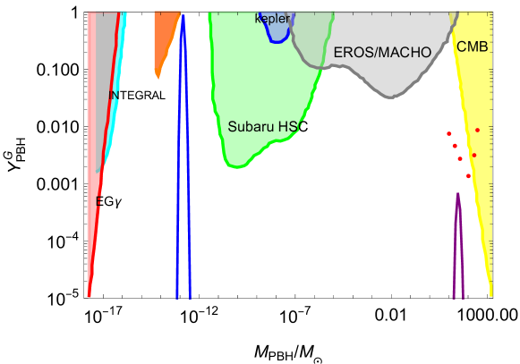
Figure 4: The PBH abundances for Model H1 (the purple line) and Model H2 (the blue line) using the Gaussian formulate $\beta^{G}$ for the fraction energy density of PBHs at the formation. The shaded regions show the observational constraints on the PBH abundance:the red region from extragalactic gamma-rays by PBH evaporation (EG$\gamma$) Carr et al. (2010), the cyan region from galactic center 511 keV gamma-ray line (INTEGRAL) Laha (2019); Dasgupta et al. (2020), the orange region from white dwarf explosion (WD) Graham et al. (2015), the green region from microlensing events with Subaru HSC Niikura et al. (2019), the blue region from the Kepler satellite Griest et al. (2013), the gray region from the EROS/MACHO Tisserand et al. (2007), the red points from LIGO merger rate Ali-Haïmoud et al. (2017) and the yellow region from accretion constraints by CMB Ali-Haïmoud and Kamionkowski (2017); Poulin et al. (2017).

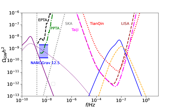
Figure 5: The SIGWs from Model H1 (the purple line), Model H2 (the blue line), WH (the purple dotted line) and Q (the orange dashed line). The black dashed curve shows the EPTA limit Ferdman et al. (2010); Hobbs et al. (2010); McLaughlin (2013); Hobbs (2013) , the grey dotted curve denotes the SKA limit Moore et al. (2015), the brown dashed curve shows the LISA limit Amaro-Seoane et al. (2017), the red dot-dashed curve denotes the TianQin limit Luo et al. (2016) and the dotted magenta curve denotes the TaiJi limit Hu and Wu (2017)

IV Primordial non-Gaussianity

Due to the violation of the slow-roll condition, the non-Gaussianity may be large. Thus it is necessary to investigate the impact of non-Gaussianity on PBH abundance and SIGWs. In this section, we first compute the primordial non-Gaussianity from our model and then we discuss its effects on PBH abundance and the energy density of SIGWs.

The non-Gaussianity parameter $f_{\text{NL}}$ is Byrnes et al. (2010)

$$f_{\text{NL}}(k_{1},k_{2},k_{3})=\frac{5}{6}\frac{B_{\zeta}(k_{1},k_{2},k_{3})}{P_{\zeta}(k_{1})P_{\zeta}(k_{2})+P_{\zeta}(k_{2})P_{\zeta}(k_{3})+P_{\zeta}(k_{3})P_{\zeta}(k_{1})},$$ (27)

where $P_{\zeta}(k)=2\pi^{2}\mathcal{P}_{\zeta}(k)/k^{3}$ and the bispectrum is defined as

$$\left\langle\hat{\zeta}_{\bm{k}_{1}}\hat{\zeta}_{\bm{k}_{2}}\hat{\zeta}_{\bm{k}_{3}}\right\rangle=(2\pi)^{3}\delta^{3}\left(\bm{k}_{1}+\bm{k}_{2}+\bm{k}_{3}\right)B_{\zeta}\left(k_{1},k_{2},k_{3}\right).$$ (28)

The expression for bispectrum is presented in Appendix.A.

With the parameter sets in table 1, we numerically compute the non-Gaussianity parameter $f_{\text{NL}}$ and the results are shown in Figs. 6 and 7. For single-field inflation, there is a consistency relation Maldacena (2003); Creminelli and Zaldarriaga (2004) that relates the bispectrum and power spectrum,

$$\lim_{k_{3}\rightarrow 0}f_{\mathrm{NL}}(k_{1},k_{2},k_{3})=\frac{5}{12}(1-n_{\mathrm{s}}),\quad\text{for}~{}k_{1}=k_{2},$$ (29)

which can be used to test our numerical computation of non-Gaussianity. From Figs. 6 and 7, we can see that the spectrum index $n_{s}-1$ matches with $-12f_{\text{NL}}/5$ in squeezed limit. Note that from the expressions for bispectrum eqs. (39)(42), the large non-Gaussianity parameter $f_{\text{NL}}$ may originate from the dramatic change in the velocity and acceleration of the inflaton. Note that the second slow-roll parameter $\epsilon_{2}$ for H1 ($q=1$, sharp power spectrum) changes more dramatically than WH ($q=6/5$, broad power spectrum) around the peak scale. Thus the non-Gaussianity parameter of WH around the peak region always stays smaller than H1, as shown in Table.5.

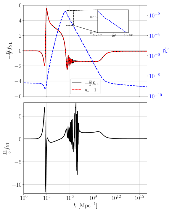
Figure 6: The power spectrum of primordial curvature perturbation and the non-Gaussianity parameter $f_{\mathrm{NL}}$ for the model H1. We show the power spectrum with the blue dashed line, $-12f_{\mathrm{NL}}/5$ in the squeezed limit with the solid black line for the modes $k_{1}=k_{2}=10^{6}k_{3}=k$ and the scalar spectral tilt $n_{\mathrm{s}}-1$ with the red dashed line in the upper panel. The insets show the oscillations in $\mathcal{P}_{\zeta}$. The lower panel shows $12f_{\mathrm{NL}}/5$ in the equilateral limit for the modes $k_{1}=k_{2}=k_{3}=k$.

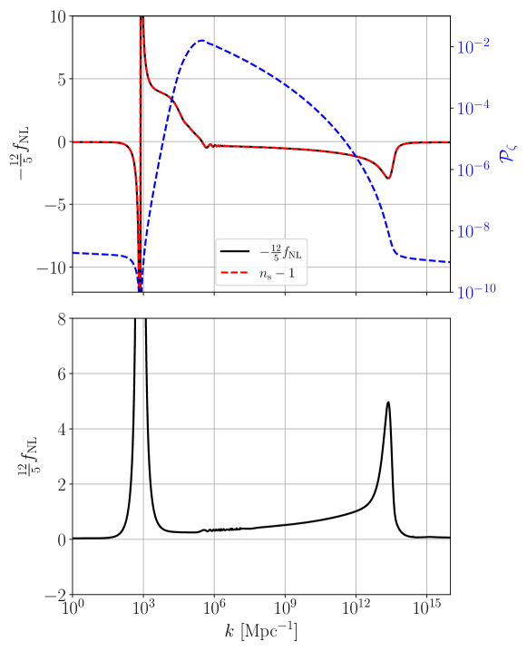
Figure 7: The power spectrum of primordial curvature perturbation and the non-Gaussianity parameter $f_{\mathrm{NL}}$ for the model WH. We show $-12f_{\mathrm{NL}}/5$ in the squzeed limit with the solid black line for the modes $k_{1}=k_{2}=10^{6}k_{3}=k$ and $12f_{\mathrm{NL}}/5$ in the equilateral limit for the modes $k_{1}=k_{2}=k_{3}=k$ in the upper and lower panels, respectively. We also show the power spectrum with the blue dashed line and the scalar spectral tilt $n_{\mathrm{s}}-1$ with the red dashed line in the upper panel.

IV.1 Non-Gaussian effect on PBH abundance

Now let us consider the non-Gaussian effect on PBH abundance. Taking the non-Gaussianity correction into account, the fraction energy density of PBH at the formation becomes Franciolini et al. (2018); Kehagias et al. (2019); Atal and Germani (2019); Riccardi et al. (2021)

$$\beta=\text{e}^{\Delta_{3}}\beta^{G}.$$ (30)

The mass of PBHs we consider is almost monochromatic, thus the third cumulant $\Delta_{3}$ can be approximately expressed as Zhang et al. (2021b)

$$\begin{split}\Delta_{3}\approx 23\frac{\delta^{3}_{c}}{\mathcal{P}_{\zeta}(k_{\text{peak}})}f_{\mathrm{NL}}(k_{\text{peak}},k_{\text{peak}},k_{\text{peak}}).\end{split}$$ (31)

In Table.5, we show the results for the non-Gaussianity parameter $f_{\text{NL}}$ and the third cumulant $\Delta_{3}$. The non-Gaussianity parameter $f_{\text{NL}}$ is of order $\mathcal{O}(10^{-1})$. In fact, during inflation with the sharper peak, the velocity of the inflaton changes more dramatically such that the non-Gaussianity effect is more significant than inflation with the broad peak. The non-Gaussianity correction has a significant enhancement on PBH abundance, which means the formation of PBHs is easier with the consideration of the non-Gaussianity. The PBH abundance is underestimated with Gaussian statistics. Note that in Ref.Zhang et al. (2021a), we have used the approximation formula for non-Gaussian PBH abundance proposed in Ref. Saito et al. (2008) and concluded that for K/G inflation, the non-Gaussian effect on PBH abundance can be neglected due to $J_{\text{peak}}\sim\mathcal{O}(10^{-3})\ll 1$. However, this analysis neglected the factor before $J_{\text{peak}}$, i.e. $\left(\hat{\zeta}^{5}-8\hat{\zeta}^{3}+9\hat{\zeta}\right)J_{\text{peak }}$, where $\hat{\zeta}\equiv\zeta/\sqrt{\mathcal{P}_{\zeta}\left(k_{\text{peak }}\right)}$ and $J\equiv\left\langle\zeta_{R_{M}}^{3}\right\rangle_{c}/\sigma_{R_{M}}^{3}/6$. Taking the critical value $\zeta_{c}\sim\mathcal{O}(1)$ Musco and Miller (2013); Harada et al. (2013); Young et al. (2014); Motohashi and Hu (2017); Franciolini et al. (2018) and thus $\hat{\zeta}_{c}\sim\mathcal{O}(10)$ , then we can find $\left(\hat{\zeta}_{c}^{5}-8\hat{\zeta}_{c}^{3}+9\hat{\zeta}_{c}\right)J_{\text{peak}}\sim\mathcal{O}(10^{2})$, which is large enough so that the non-Gaussian effect on PBH cannot be neglected. On the other hand, note that the formula for non-Gaussian PBH abundance in Ref.Saito et al. (2008) is an approximation result requiring the term $(\text{prefactor}\times J)\ll 1$, which is not satisfied in K/G inflation. Thus in this paper and Ref.Zhang et al. (2021b), we adopt the exact formula for non-Gaussian PBH abundance proposed in Ref.Franciolini et al. (2018).

Model	$f_{\text{NL}}(k_{\text{peak}},k_{\text{peak}},k_{\text{peak}})$	$\Delta_{3}$
H1	0.62	25
H2	0.53	30
WH	0.13	12

Table 5: The results for the non-Gaussianity parameter $f_{\text{NL}}$ and the third cumulant $\Delta_{3}$.

IV.2 Non-Gaussian effect on SIGW

To investigate the non-Gaussian effect on SIGWs, we first consider the power spectrum with the non-Gaussian correction. The comoving curvature perturvation with the nonlinear corrections can be expressed as Verde et al. (2000); Komatsu and Spergel (2001)

$$\zeta(\bm{x})=\zeta^{G}(\bm{x})+\frac{3}{5}f_{\text{NL}}(\zeta^{G}(\bm{x})^{2}-\langle\zeta^{G}(\bm{x})^{2}\rangle),$$ (32)

where $\zeta^{G}$ is the Gaussian part of the curvature perturbation. Thus the power spectrum is

$$\mathcal{P}_{\zeta}(k)=\mathcal{P}^{G}_{\zeta}(k)+\mathcal{P}^{NG}_{\zeta}(k),$$ (33)

with the non-Gaussian correction of the power spectrum

$$\mathcal{P}^{NG}_{\zeta}(k)=\left(\frac{3}{5}\right)^{2}\frac{k^{3}}{2\pi}f^{2}_{\mathrm{NL}}\int d^{3}\bm{p}\frac{\mathcal{P}^{G}_{\zeta}(p)}{p^{3}}\frac{\mathcal{P}^{G}_{\zeta}(|\bm{k}-\bm{p}|)}{|\bm{k}-\bm{p}|^{3}}.$$ (34)

For our model with $f_{\text{NL}}\sim\mathcal{O}(10^{-1})$ at peak scales, we have $\mathcal{P}^{NG}_{\zeta}(k)\ll\mathcal{P}^{G}_{\zeta}(k)$ and thus the non-Gaussian effect can be neglected when calculating SIGWs.

V Conclusions

K/G inflation with a noncanonical kinetic term $(1+G(\phi))X$ can produce enhanced curvature perturbations at small scales if the coupling function $G(\phi)$ has a peak. However, due to the dramatic decrease in $\dot{\phi}$, the peak function $G(\phi)$ will contribute up to $\sim 20$ $e$-folds and the usual slow-roll inflation epoch endures around $30\text{-}40$ $e$-folds. For power-law potential $V=\lambda\phi^{p}$, this indicates $p$ should be bounded as $p\lesssim 1$. In particular, this mechanism does not work for Higgs potential $V=\lambda\phi^{4}$. To resolve potential-restriction problem and produce PBHs and SIGWs in Higgs inflation, we introduce K/G inflation with nonminimal coupling and show that the curvature perturbation at small scales can be enhanced by the Higgs field while satisfying the constraints from CMB observations. To be specific, in the Einstein frame, the conformal factor flattens the Higgs potential such that the $e$-folds during slow-roll inflation is within $40$ and the tensor-to-scalar ratio is reduced.

We then study the non-canonical kinetic coupling function in detail. On the one hand, phenomenologically, we find that the non-canonical kinetic coupling function not only drives the dramatic decreases in $\dot{\phi}$ and thus the enhancement of the curvature perturbation but also helps the exit of inflation. On the other hand, we study the observational constraints from LIGO merger rates and the White Dwarf explosion on the parameter space of the non-canonical kinetic coupling function. Our numerical results show that for a given width parameter $c$, there is an upper bound on the amplitude parameter $h$ and as $c$ gets larger, the upper bound on $h$ decreases. The reason is that the larger $c$ indicates a wider peak function and thus the velocity of the inflaton decreases more dramatically and a smaller amplitude parameter $h$ is required to realize the same enhancement on curvature perturbations.

By varying the peak position, the curvature perturbation can be enhanced at different scales and thus different mass ranges of PBHs and frequencies of SIGWs can be produced. PBHs with mass $\mathcal{O}(10)M_{\odot},\ \mathcal{O}(10^{-12})M_{\odot}$ from models H1 and H2 may explain BHs in LIGO-Virgo events and almost all the DM, respectively. For SIGWs, we give the gauge invariant expression for the integral kernel of genuine SIGWs, which is related to terms propagating with the speed of light. The energy density of SIGWs from the model WH lies within the $2\sigma$ region of the NANOGrav signal. Thus NANOGrav signal may originate from the Higgs field. SIGWs from the model H2 have the millihertz frequency, which can be tested by future space-based detectors like LISA, TaiJi, and TianQin.

Due to the violation of the slow-roll condition, the non-Gaussianity may have a significant effect on PBH abundance and SIGWs. Around the peak scale, we find that the non-Gaussianity parameter $f_{\text{NL}}$ of sharp power spectrum is larger than that of broad power spectrum due to more dramatic change in the velocity of the inflaton. For our models, the non-Gaussianity parameter $f_{\text{NL}}$ in the equilateral limit is of order $\mathcal{O}(10^{-1})$ at peak scales and the non-Gaussianity correction has a significant enhancement on PBH abundance. Notwithstanding, the energy density of SIGWs remains invariant even if we take the non-Gaussianity into account, as the power spectrum receives very tiny corrections.

Appendix A The expression for the bispectrum

The bispectrum $B_{\zeta}(k_{1},k_{2},k_{3})$ is Hazra et al. (2013); Ragavendra et al. (2020); Arroja and Tanaka (2011)

$$B_{\zeta}(k_{1},k_{2},k_{3})=\Sigma^{10}_{i=1}B^{i}_{\zeta}(k_{1},k_{2},k_{3}),$$ (35)

$$\begin{split}B^{1}_{\zeta}(k_{1},k_{2},k_{3})=&-4\operatorname{Im}\left[\zeta_{{k}_{1}}(\tau_{*})\zeta_{{k}_{2}}(\tau_{*})\zeta_{{k}_{3}}(\tau_{*})\int_{\tau_{i}}^{\tau_{*}}d\tau a^{2}\epsilon_{1}^{2}\left\{\zeta^{*}_{{k}_{1}}(\tau)\zeta^{{}^{\prime}*}_{{k}_{2}}(\tau)\zeta^{{}^{\prime}*}_{{k}_{3}}(\tau)+\mathrm{perm}\right\}\right],\end{split}$$ (36)

$$\begin{split}B^{2}_{\zeta}(k_{1},k_{2},k_{3})=&2\operatorname{Im}\left[\vphantom{\left(\frac{\bm{k}_{2}\cdot\bm{k}_{3}}{k_{3}}\right)^{2}}\zeta_{{k}_{1}}(\tau_{*})\zeta_{{k}_{2}}(\tau_{*})\zeta_{{k}_{3}}(\tau_{*})\right.\\ &\left.\int_{\tau_{i}}^{\tau_{*}}d\tau a^{2}\epsilon_{1}^{2}\left\{(k^{2}_{1}-k^{2}_{2}-k^{2}_{3})\zeta^{*}_{{k}_{1}}(\tau)\zeta^{*}_{{k}_{2}}(\tau)\zeta^{*}_{{k}_{3}}(\tau)+\mathrm{perm}\right\}\right],\end{split}$$ (37)

$$\begin{split}B^{3}_{\zeta}(k_{1},k_{2},k_{3})=&2\operatorname{Im}\left[\vphantom{\left(\frac{\bm{k}_{2}\cdot\bm{k}_{3}}{k_{3}}\right)^{2}}\zeta_{{k}_{1}}(\tau_{*})\zeta_{{k}_{2}}(\tau_{*})\zeta_{{k}_{3}}(\tau_{*})\right.\\ &\left.\int_{\tau_{i}}^{\tau_{*}}d\tau a^{2}\epsilon_{1}^{2}\left\{\left(\frac{k^{2}_{2}-k^{2}_{1}-k^{2}_{3}}{k^{2}_{1}}+\frac{k^{2}_{1}-k^{2}_{2}-k^{2}_{3}}{k^{2}_{2}}\right)\zeta^{{}^{\prime}*}_{{k}_{1}}(\tau)\zeta^{{}^{\prime}*}_{{k}_{2}}(\tau)\zeta^{*}_{{k}_{3}}(\tau)+\mathrm{perm}\right\}\right],\end{split}$$ (38)

$$B^{4}_{\zeta}(k_{1},k_{2},k_{3})=-2\operatorname{Im}\left[\zeta_{{k}_{1}}(\tau_{*})\zeta_{{k}_{2}}(\tau_{*})\zeta_{{k}_{3}}(\tau_{*})\int_{\tau_{i}}^{\tau_{*}}d\tau a^{2}\epsilon_{1}\eta^{\prime}\left\{\zeta^{*}_{{k}_{1}}(\tau)\zeta^{*}_{{k}_{2}}(\tau)\zeta^{{}^{\prime}*}_{{k}_{3}}(\tau)+\mathrm{perm}\right\}\right],$$ (39)

$$\begin{split}B^{5}_{\zeta}(k_{1},k_{2},k_{3})=&-\frac{1}{2}\operatorname{Im}\left[\vphantom{\left(\frac{\bm{k}_{2}\cdot\bm{k}_{3}}{k_{3}}\right)^{2}}\zeta_{{k}_{1}}(\tau_{*})\zeta_{{k}_{2}}(\tau_{*})\zeta_{{k}_{3}}(\tau_{*})\right.\\ &\left.\int_{\tau_{i}}^{\tau_{*}}d\tau a^{2}\epsilon_{1}^{3}\left\{\left(\frac{k^{2}_{2}-k^{2}_{1}-k^{2}_{3}}{k^{2}_{1}}+\frac{k^{2}_{1}-k^{2}_{2}-k^{2}_{3}}{k^{2}_{2}}\right)\zeta^{{}^{\prime}*}_{{k}_{1}}(\tau)\zeta^{{}^{\prime}*}_{{k}_{2}}(\tau)\zeta^{*}_{{k}_{3}}(\tau)+\mathrm{perm}\right\}\right],\end{split}$$ (40)

$$\begin{split}B^{6}_{\zeta}(k_{1},k_{2},k_{3})=&-\frac{1}{2}\operatorname{Im}\left[\vphantom{\left(\frac{\bm{k}_{2}\cdot\bm{k}_{3}}{k_{3}}\right)^{2}}\zeta_{{k}_{1}}(\tau_{*})\zeta_{{k}_{2}}(\tau_{*})\zeta_{{k}_{3}}(\tau_{*})\right.\\ &\left.\int_{\tau_{i}}^{\tau_{*}}d\tau a^{2}\epsilon_{1}^{3}\left\{\frac{k^{2}_{3}\left(k^{2}_{3}-k^{2}_{1}-k^{2}_{2}\right)}{k^{2}_{1}k^{2}_{2}}\zeta^{{}^{\prime}*}_{{k}_{1}}(\tau)\zeta^{{}^{\prime}*}_{{k}_{2}}(\tau)\zeta^{*}_{{k}_{3}}(\tau)+\mathrm{perm}\right\}\right],\end{split}$$ (41)

$$B^{7}_{\zeta}(k_{1},k_{2},k_{3})=2\operatorname{Im}\left[\zeta_{k_{1}}(\tau_{*})\zeta_{k_{2}}(\tau_{*})\zeta_{k_{3}}(\tau_{*})\left(a^{2}\epsilon_{1}\eta\zeta_{k_{1}}^{*}(\tau)\zeta_{k_{2}}^{*}(\tau)\zeta_{k_{3}}^{\prime*}(\tau)+\mathrm{perm}\right)\right]\Big{|}_{\tau_{i}}^{\tau_{*}},$$ (42)

$$\begin{split}B^{8}_{\zeta}(k_{1},k_{2},k_{3})=&2\operatorname{Im}\left[\zeta_{k_{1}}(\tau_{*})\zeta_{k_{2}}(\tau_{*})\zeta_{k_{3}}(\tau_{*})\times\left(\frac{a}{H}\zeta_{k_{1}}^{*}(\tau)\zeta_{k_{2}}^{*}(\tau)\zeta_{k_{3}}^{*}(\tau)\right)\right.\\ &\left.\times\left\{54(aH)^{2}+2(1-\epsilon_{1})(\bm{k}_{1}\cdot\bm{k}_{2}+\mathrm{perm})+\right.\right.\\ &\left.\left.\frac{1}{2(aH)^{2}}\left[\left(\bm{k}_{1}\cdot\bm{k}_{2}\right)k_{3}^{2}+\mathrm{perm}\right]\right\}\right]\Big{|}_{\tau_{i}}^{\tau_{*}},\end{split}$$ (43)

$$\begin{split}B^{9}_{\zeta}(k_{1},k_{2},k_{3})=&-\operatorname{Im}\left[\vphantom{\left(\frac{\bm{k}_{2}\cdot\bm{k}_{3}}{k_{3}}\right)^{2}}\zeta_{k_{1}}(\tau_{*})\zeta_{k_{2}}(\tau_{*})\zeta_{k_{3}}(\tau_{*})\left\{\frac{\epsilon_{1}}{H^{2}}\zeta_{k_{1}}^{*}(\tau)\zeta_{k_{2}}^{*}(\tau)\zeta_{k_{3}}^{\prime*}(\tau)\right.\right.\\ &\left.\left.\left[k_{1}^{2}+k_{2}^{2}-\left(\frac{\bm{k}_{1}\cdot\bm{k}_{3}}{k_{3}}\right)^{2}-\left(\frac{\bm{k}_{2}\cdot\bm{k}_{3}}{k_{3}}\right)^{2}\right]+\mathrm{perm}\right\}\right]\Big{|}^{\tau_{*}}_{\tau_{i}},\end{split}$$ (44)

$$\begin{split}B^{10}_{\zeta}(k_{1},k_{2},k_{3})=&2\operatorname{Im}\left[\vphantom{\left(\frac{\bm{k}_{2}\cdot\bm{k}_{3}}{k_{3}}\right)^{2}}\zeta_{k_{1}}(\tau_{*})\zeta_{k_{2}}(\tau_{*})\zeta_{k_{3}}(\tau_{*})\right.\\ &\left.\left.\times\left\{\frac{a\epsilon_{1}}{H}\zeta_{k_{1}}^{*}(\tau)\zeta_{k_{2}}^{\prime*}(\tau)\zeta_{k_{3}}^{\prime*}(\tau)\left[2-\epsilon_{1}+\epsilon_{1}\left(\frac{\bm{k}_{2}\cdot\bm{k}_{3}}{k_{2}k_{3}}\right)^{2}\right]+\mathrm{perm}\right\}\right]\right|^{\tau_{*}}_{\tau_{i}},\end{split}$$ (45)

where

$$\eta=\dot{\epsilon}_{1}/H\epsilon_{1},$$

$\tau_{i}$ is the early time when all relevant modes are well within the horizon and the plane-wave initial condition is imposed. $\tau_{*}$ is the late time when all relevant modes have been frozen.

References

- Carr and Hawking (1974) B. J. Carr and S. W. Hawking, Mon. Not. Roy. Astron. Soc. 168, 399 (1974).
- Hawking (1971) S. Hawking, Mon. Not. Roy. Astron. Soc. 152, 75 (1971).
- Ivanov et al. (1994) P. Ivanov, P. Naselsky, and I. Novikov, Phys. Rev. D 50, 7173 (1994).
- Frampton et al. (2010) P. H. Frampton, M. Kawasaki, F. Takahashi, and T. T. Yanagida, JCAP 04, 023 (2010), arXiv:1001.2308 [hep-ph] .
- Belotsky et al. (2014) K. M. Belotsky, A. D. Dmitriev, E. A. Esipova, V. A. Gani, A. V. Grobov, M. Y. Khlopov, A. A. Kirillov, S. G. Rubin, and I. V. Svadkovsky, Mod. Phys. Lett. A 29, 1440005 (2014), arXiv:1410.0203 [astro-ph.CO] .
- Khlopov et al. (2005) M. Y. Khlopov, S. G. Rubin, and A. S. Sakharov, Astropart. Phys. 23, 265 (2005), arXiv:astro-ph/0401532 .
- Clesse and García-Bellido (2015) S. Clesse and J. García-Bellido, Phys. Rev. D 92, 023524 (2015), arXiv:1501.07565 [astro-ph.CO] .
- Carr et al. (2016) B. Carr, F. Kuhnel, and M. Sandstad, Phys. Rev. D 94, 083504 (2016), arXiv:1607.06077 [astro-ph.CO] .
- Inomata et al. (2017a) K. Inomata, M. Kawasaki, K. Mukaida, Y. Tada, and T. T. Yanagida, Phys. Rev. D 96, 043504 (2017a), arXiv:1701.02544 [astro-ph.CO] .
- García-Bellido (2017) J. García-Bellido, J. Phys. Conf. Ser. 840, 012032 (2017), arXiv:1702.08275 [astro-ph.CO] .
- Kovetz (2017) E. D. Kovetz, Phys. Rev. Lett. 119, 131301 (2017), arXiv:1705.09182 [astro-ph.CO] .
- Abbott et al. (2016a) B. P. Abbott et al. (LIGO Scientific, Virgo), Phys. Rev. Lett. 116, 061102 (2016a), arXiv:1602.03837 [gr-qc] .
- Abbott et al. (2016b) B. P. Abbott et al. (LIGO Scientific, Virgo), Phys. Rev. Lett. 116, 241103 (2016b), arXiv:1606.04855 [gr-qc] .
- Bird et al. (2016) S. Bird, I. Cholis, J. B. Muñoz, Y. Ali-Haïmoud, M. Kamionkowski, E. D. Kovetz, A. Raccanelli, and A. G. Riess, Phys. Rev. Lett. 116, 201301 (2016), arXiv:1603.00464 [astro-ph.CO] .
- Sasaki et al. (2016) M. Sasaki, T. Suyama, T. Tanaka, and S. Yokoyama, Phys. Rev. Lett. 117, 061101 (2016), [Erratum: Phys.Rev.Lett. 121, 059901 (2018)], arXiv:1603.08338 [astro-ph.CO] .
- Sato-Polito et al. (2019) G. Sato-Polito, E. D. Kovetz, and M. Kamionkowski, Phys. Rev. D 100, 063521 (2019), arXiv:1904.10971 [astro-ph.CO] .
- Akrami et al. (2020) Y. Akrami et al. (Planck), Astron. Astrophys. 641, A10 (2020), arXiv:1807.06211 [astro-ph.CO] .
- Germani and Prokopec (2017) C. Germani and T. Prokopec, Phys. Dark Univ. 18, 6 (2017), arXiv:1706.04226 [astro-ph.CO] .
- Motohashi and Hu (2017) H. Motohashi and W. Hu, Phys. Rev. D 96, 063503 (2017), arXiv:1706.06784 [astro-ph.CO] .
- Di and Gong (2018) H. Di and Y. Gong, JCAP 07, 007 (2018), arXiv:1707.09578 [astro-ph.CO] .
- Wu et al. (2021) L. Wu, Y. Gong, and T. Li, (2021), arXiv:2105.07694 [gr-qc] .
- Inomata et al. (2021a) K. Inomata, E. McDonough, and W. Hu, (2021a), arXiv:2110.14641 [astro-ph.CO] .
- Fu et al. (2019) C. Fu, P. Wu, and H. Yu, Phys. Rev. D 100, 063532 (2019), arXiv:1907.05042 [astro-ph.CO] .
- Kawai and Kim (2021) S. Kawai and J. Kim, Phys. Rev. D 104, 083545 (2021), arXiv:2108.01340 [astro-ph.CO] .
- Chen et al. (2021) P. Chen, S. Koh, and G. Tumurtushaa, (2021), arXiv:2107.08638 [gr-qc] .
- Teimoori et al. (2021) Z. Teimoori, K. Rezazadeh, M. A. Rasheed, and K. Karami, (2021), 10.1088/1475-7516/2021/10/018, arXiv:2107.07620 [astro-ph.CO] .
- Liu and Xu (2021) L.-H. Liu and W.-L. Xu, (2021), arXiv:2107.07310 [astro-ph.CO] .
- Zheng et al. (2021) R. Zheng, J. Shi, and T. Qiu, (2021), arXiv:2106.04303 [astro-ph.CO] .
- Heydari and Karami (2021a) S. Heydari and K. Karami, (2021a), arXiv:2107.10550 [gr-qc] .
- Heydari and Karami (2021b) S. Heydari and K. Karami, (2021b), arXiv:2111.00494 [gr-qc] .
- Cai et al. (2021a) R.-G. Cai, C. Chen, and C. Fu, Phys. Rev. D 104, 083537 (2021a), arXiv:2108.03422 [astro-ph.CO] .
- Wang et al. (2021) Q. Wang, Y.-C. Liu, B.-Y. Su, and N. Li, Phys. Rev. D 104, 083546 (2021).
- Ahmed et al. (2021) W. Ahmed, M. Junaid, and U. Zubair, (2021), arXiv:2109.14838 [astro-ph.CO] .
- Sasaki et al. (2018) M. Sasaki, T. Suyama, T. Tanaka, and S. Yokoyama, Class. Quant. Grav. 35, 063001 (2018), arXiv:1801.05235 [astro-ph.CO] .
- Passaglia et al. (2019) S. Passaglia, W. Hu, and H. Motohashi, Phys. Rev. D 99, 043536 (2019), arXiv:1812.08243 [astro-ph.CO] .
- Lin et al. (2020) J. Lin, Q. Gao, Y. Gong, Y. Lu, C. Zhang, and F. Zhang, Phys. Rev. D 101, 103515 (2020), arXiv:2001.05909 [gr-qc] .
- Yi et al. (2021a) Z. Yi, Y. Gong, B. Wang, and Z.-h. Zhu, Phys. Rev. D 103, 063535 (2021a), arXiv:2007.09957 [gr-qc] .
- Yi et al. (2021b) Z. Yi, Q. Gao, Y. Gong, and Z.-h. Zhu, Phys. Rev. D 103, 063534 (2021b), arXiv:2011.10606 [astro-ph.CO] .
- Gao et al. (2021) Q. Gao, Y. Gong, and Z. Yi, Nucl. Phys. B 969, 115480 (2021), arXiv:2012.03856 [gr-qc] .
- Yi and Zhu (2021) Z. Yi and Z.-H. Zhu, (2021), arXiv:2105.01943 [gr-qc] .
- Zhang et al. (2021a) F. Zhang, Y. Gong, J. Lin, Y. Lu, and Z. Yi, JCAP 04, 045 (2021a), arXiv:2012.06960 [astro-ph.CO] .
- Zhang et al. (2021b) F. Zhang, J. Lin, and Y. Lu, Phys. Rev. D 104, 063515 (2021b), [Erratum: Phys.Rev.D 104, 129902 (2021)], arXiv:2106.10792 [gr-qc] .
- Solbi and Karami (2021) M. Solbi and K. Karami, JCAP 08, 056 (2021), arXiv:2102.05651 [astro-ph.CO] .
- Kaiser (1995) D. I. Kaiser, Phys. Rev. D 52, 4295 (1995), arXiv:astro-ph/9408044 .
- Bezrukov and Shaposhnikov (2008) F. L. Bezrukov and M. Shaposhnikov, Phys. Lett. B 659, 703 (2008), arXiv:0710.3755 [hep-th] .
- Germani and Kehagias (2010) C. Germani and A. Kehagias, Phys. Rev. Lett. 105, 011302 (2010), arXiv:1003.2635 [hep-ph] .
- Germani et al. (2014) C. Germani, Y. Watanabe, and N. Wintergerst, JCAP 12, 009 (2014), arXiv:1403.5766 [hep-ph] .
- Hamada et al. (2014) Y. Hamada, H. Kawai, K.-y. Oda, and S. C. Park, Phys. Rev. Lett. 112, 241301 (2014), arXiv:1403.5043 [hep-ph] .
- Yang et al. (2016) N. Yang, Q. Fei, Q. Gao, and Y. Gong, Class. Quant. Grav. 33, 205001 (2016), arXiv:1504.05839 [gr-qc] .
- Fumagalli et al. (2018) J. Fumagalli, S. Mooij, and M. Postma, JHEP 03, 038 (2018), arXiv:1711.08761 [hep-ph] .
- Fumagalli et al. (2020) J. Fumagalli, M. Postma, and M. Van Den Bout, JHEP 09, 114 (2020), arXiv:2005.05905 [hep-ph] .
- Ezquiaga et al. (2018) J. M. Ezquiaga, J. Garcia-Bellido, and E. Ruiz Morales, Phys. Lett. B 776, 345 (2018), arXiv:1705.04861 [astro-ph.CO] .
- Bezrukov et al. (2018) F. Bezrukov, M. Pauly, and J. Rubio, JCAP 02, 040 (2018), arXiv:1706.05007 [hep-ph] .
- Matarrese et al. (1998) S. Matarrese, S. Mollerach, and M. Bruni, Phys. Rev. D 58, 043504 (1998), arXiv:astro-ph/9707278 .
- Mollerach et al. (2004) S. Mollerach, D. Harari, and S. Matarrese, Phys. Rev. D 69, 063002 (2004), arXiv:astro-ph/0310711 .
- Ananda et al. (2007) K. N. Ananda, C. Clarkson, and D. Wands, Phys. Rev. D 75, 123518 (2007), arXiv:gr-qc/0612013 .
- Baumann et al. (2007) D. Baumann, P. J. Steinhardt, K. Takahashi, and K. Ichiki, Phys. Rev. D 76, 084019 (2007), arXiv:hep-th/0703290 .
- Garcia-Bellido et al. (2017) J. Garcia-Bellido, M. Peloso, and C. Unal, JCAP 09, 013 (2017), arXiv:1707.02441 [astro-ph.CO] .
- Saito and Yokoyama (2009) R. Saito and J. Yokoyama, Phys. Rev. Lett. 102, 161101 (2009), [Erratum: Phys.Rev.Lett. 107, 069901 (2011)], arXiv:0812.4339 [astro-ph] .
- Saito and Yokoyama (2010) R. Saito and J. Yokoyama, Prog. Theor. Phys. 123, 867 (2010), [Erratum: Prog.Theor.Phys. 126, 351–352 (2011)], arXiv:0912.5317 [astro-ph.CO] .
- Bugaev and Klimai (2010) E. Bugaev and P. Klimai, Phys. Rev. D 81, 023517 (2010), arXiv:0908.0664 [astro-ph.CO] .
- Bugaev and Klimai (2011) E. Bugaev and P. Klimai, Phys. Rev. D 83, 083521 (2011), arXiv:1012.4697 [astro-ph.CO] .
- Alabidi et al. (2012) L. Alabidi, K. Kohri, M. Sasaki, and Y. Sendouda, JCAP 09, 017 (2012), arXiv:1203.4663 [astro-ph.CO] .
- Orlofsky et al. (2017) N. Orlofsky, A. Pierce, and J. D. Wells, Phys. Rev. D 95, 063518 (2017), arXiv:1612.05279 [astro-ph.CO] .
- Nakama et al. (2017) T. Nakama, J. Silk, and M. Kamionkowski, Phys. Rev. D 95, 043511 (2017), arXiv:1612.06264 [astro-ph.CO] .
- Inomata et al. (2017b) K. Inomata, M. Kawasaki, K. Mukaida, Y. Tada, and T. T. Yanagida, Phys. Rev. D 95, 123510 (2017b), arXiv:1611.06130 [astro-ph.CO] .
- Cheng et al. (2018) S.-L. Cheng, W. Lee, and K.-W. Ng, JCAP 07, 001 (2018), arXiv:1801.09050 [astro-ph.CO] .
- Cai et al. (2019a) R.-G. Cai, S. Pi, S.-J. Wang, and X.-Y. Yang, JCAP 05, 013 (2019a), arXiv:1901.10152 [astro-ph.CO] .
- Cai et al. (2020) R.-G. Cai, Z.-K. Guo, J. Liu, L. Liu, and X.-Y. Yang, JCAP 06, 013 (2020), arXiv:1912.10437 [astro-ph.CO] .
- Cai et al. (2019b) R.-G. Cai, S. Pi, S.-J. Wang, and X.-Y. Yang, JCAP 10, 059 (2019b), arXiv:1907.06372 [astro-ph.CO] .
- Domènech (2021) G. Domènech, Universe 7, 398 (2021), arXiv:2109.01398 [gr-qc] .
- Ferdman et al. (2010) R. D. Ferdman et al., Class. Quant. Grav. 27, 084014 (2010), arXiv:1003.3405 [astro-ph.HE] .
- Hobbs et al. (2010) G. Hobbs et al., Class. Quant. Grav. 27, 084013 (2010), arXiv:0911.5206 [astro-ph.SR] .
- McLaughlin (2013) M. A. McLaughlin, Class. Quant. Grav. 30, 224008 (2013), arXiv:1310.0758 [astro-ph.IM] .
- Hobbs (2013) G. Hobbs, Class. Quant. Grav. 30, 224007 (2013), arXiv:1307.2629 [astro-ph.IM] .
- Amaro-Seoane et al. (2017) P. Amaro-Seoane et al. (LISA), (2017), arXiv:1702.00786 [astro-ph.IM] .
- Hu and Wu (2017) W.-R. Hu and Y.-L. Wu, Natl. Sci. Rev. 4, 685 (2017).
- Luo et al. (2016) J. Luo et al. (TianQin), Class. Quant. Grav. 33, 035010 (2016), arXiv:1512.02076 [astro-ph.IM] .
- Brans and Dicke (1961) C. Brans and R. H. Dicke, Phys. Rev. 124, 925 (1961).
- Ade et al. (2021) P. A. R. Ade et al. (BICEP, Keck), Phys. Rev. Lett. 127, 151301 (2021), arXiv:2110.00483 [astro-ph.CO] .
- Fixsen et al. (1996) D. J. Fixsen, E. S. Cheng, J. M. Gales, J. C. Mather, R. A. Shafer, and E. L. Wright, Astrophys. J. 473, 576 (1996), arXiv:astro-ph/9605054 .
- Inomata et al. (2016) K. Inomata, M. Kawasaki, and Y. Tada, Phys. Rev. D 94, 043527 (2016), arXiv:1605.04646 [astro-ph.CO] .
- Inomata and Nakama (2019) K. Inomata and T. Nakama, Phys. Rev. D 99, 043511 (2019), arXiv:1812.00674 [astro-ph.CO] .
- Ali-Haïmoud et al. (2017) Y. Ali-Haïmoud, E. D. Kovetz, and M. Kamionkowski, Phys. Rev. D 96, 123523 (2017), arXiv:1709.06576 [astro-ph.CO] .
- Graham et al. (2015) P. W. Graham, S. Rajendran, and J. Varela, Phys. Rev. D 92, 063007 (2015), arXiv:1505.04444 [hep-ph] .
- Lu et al. (2020) Y. Lu, A. Ali, Y. Gong, J. Lin, and F. Zhang, Phys. Rev. D 102, 083503 (2020), arXiv:2006.03450 [gr-qc] .
- Kohri and Terada (2018) K. Kohri and T. Terada, Phys. Rev. D 97, 123532 (2018), arXiv:1804.08577 [gr-qc] .
- Espinosa et al. (2018) J. R. Espinosa, D. Racco, and A. Riotto, JCAP 09, 012 (2018), arXiv:1804.07732 [hep-ph] .
- Lu et al. (2019) Y. Lu, Y. Gong, Z. Yi, and F. Zhang, JCAP 12, 031 (2019), arXiv:1907.11896 [gr-qc] .
- Hwang et al. (2017) J.-C. Hwang, D. Jeong, and H. Noh, Astrophysical Journal 842, 46 (2017), arXiv:1704.03500 [astro-ph.CO] .
- Tomikawa and Kobayashi (2020) K. Tomikawa and T. Kobayashi, Physical Review D 101, 083529 (2020), arXiv:1910.01880 [gr-qc] .
- Ali et al. (2021) A. Ali, Y. Gong, and Y. Lu, Phys. Rev. D 103, 043516 (2021), arXiv:2009.11081 [gr-qc] .
- De Luca et al. (2020) V. De Luca, G. Franciolini, A. Kehagias, and A. Riotto, JCAP 03, 014 (2020), arXiv:1911.09689 [gr-qc] .
- Inomata and Terada (2020) K. Inomata and T. Terada, Phys. Rev. D 101, 023523 (2020), arXiv:1912.00785 [gr-qc] .
- Yuan et al. (2020) C. Yuan, Z.-C. Chen, and Q.-G. Huang, Phys. Rev. D 101, 063018 (2020), arXiv:1912.00885 [astro-ph.CO] .
- Domènech and Sasaki (2021) G. Domènech and M. Sasaki, Phys. Rev. D 103, 063531 (2021), arXiv:2012.14016 [gr-qc] .
- Chang et al. (2020) Z. Chang, S. Wang, and Q.-H. Zhu, (2020), arXiv:2009.11994 [gr-qc] .
- Cai et al. (2021b) R.-G. Cai, X.-Y. Yang, and L. Zhao, (2021b), arXiv:2109.06865 [astro-ph.CO] .
- Carr (1975) B. J. Carr, Astrophys. J. 201, 1 (1975).
- Aghanim et al. (2020) N. Aghanim et al. (Planck), Astron. Astrophys. 641, A6 (2020), [Erratum: Astron.Astrophys. 652, C4 (2021)], arXiv:1807.06209 [astro-ph.CO] .
- Özsoy et al. (2018) O. Özsoy, S. Parameswaran, G. Tasinato, and I. Zavala, JCAP 07, 005 (2018), arXiv:1803.07626 [hep-th] .
- Tada and Yokoyama (2019) Y. Tada and S. Yokoyama, Phys. Rev. D 100, 023537 (2019), arXiv:1904.10298 [astro-ph.CO] .
- Musco and Miller (2013) I. Musco and J. C. Miller, Class. Quant. Grav. 30, 145009 (2013), arXiv:1201.2379 [gr-qc] .
- Harada et al. (2013) T. Harada, C.-M. Yoo, and K. Kohri, Phys. Rev. D 88, 084051 (2013), [Erratum: Phys.Rev.D 89, 029903 (2014)], arXiv:1309.4201 [astro-ph.CO] .
- Escrivà et al. (2020) A. Escrivà, C. Germani, and R. K. Sheth, Phys. Rev. D 101, 044022 (2020), arXiv:1907.13311 [gr-qc] .
- Yoo et al. (2020) C.-M. Yoo, T. Harada, and H. Okawa, Phys. Rev. D 102, 043526 (2020), arXiv:2004.01042 [gr-qc] .
- De Luca et al. (2021) V. De Luca, G. Franciolini, and A. Riotto, Phys. Rev. Lett. 126, 041303 (2021), arXiv:2009.08268 [astro-ph.CO] .
- Inomata et al. (2021b) K. Inomata, M. Kawasaki, K. Mukaida, and T. T. Yanagida, Phys. Rev. Lett. 126, 131301 (2021b), arXiv:2011.01270 [astro-ph.CO] .
- Vaskonen and Veermäe (2021) V. Vaskonen and H. Veermäe, Phys. Rev. Lett. 126, 051303 (2021), arXiv:2009.07832 [astro-ph.CO] .
- Kohri and Terada (2021) K. Kohri and T. Terada, Phys. Lett. B 813, 136040 (2021), arXiv:2009.11853 [astro-ph.CO] .
- Domènech and Pi (2020) G. Domènech and S. Pi, (2020), arXiv:2010.03976 [astro-ph.CO] .
- Vagnozzi (2021) S. Vagnozzi, Mon. Not. Roy. Astron. Soc. 502, L11 (2021), arXiv:2009.13432 [astro-ph.CO] .
- Kawasaki and Nakatsuka (2021) M. Kawasaki and H. Nakatsuka, JCAP 05, 023 (2021), arXiv:2101.11244 [astro-ph.CO] .
- Carr et al. (2010) B. J. Carr, K. Kohri, Y. Sendouda, and J. Yokoyama, Phys. Rev. D 81, 104019 (2010), arXiv:0912.5297 [astro-ph.CO] .
- Laha (2019) R. Laha, Phys. Rev. Lett. 123, 251101 (2019), arXiv:1906.09994 [astro-ph.HE] .
- Dasgupta et al. (2020) B. Dasgupta, R. Laha, and A. Ray, Phys. Rev. Lett. 125, 101101 (2020), arXiv:1912.01014 [hep-ph] .
- Niikura et al. (2019) H. Niikura et al., Nature Astron. 3, 524 (2019), arXiv:1701.02151 [astro-ph.CO] .
- Griest et al. (2013) K. Griest, A. M. Cieplak, and M. J. Lehner, Phys. Rev. Lett. 111, 181302 (2013).
- Tisserand et al. (2007) P. Tisserand et al. (EROS-2), Astron. Astrophys. 469, 387 (2007), arXiv:astro-ph/0607207 .
- Ali-Haïmoud and Kamionkowski (2017) Y. Ali-Haïmoud and M. Kamionkowski, Phys. Rev. D 95, 043534 (2017), arXiv:1612.05644 [astro-ph.CO] .
- Poulin et al. (2017) V. Poulin, P. D. Serpico, F. Calore, S. Clesse, and K. Kohri, Phys. Rev. D 96, 083524 (2017), arXiv:1707.04206 [astro-ph.CO] .
- Moore et al. (2015) C. J. Moore, R. H. Cole, and C. P. L. Berry, Class. Quant. Grav. 32, 015014 (2015), arXiv:1408.0740 [gr-qc] .
- Byrnes et al. (2010) C. T. Byrnes, M. Gerstenlauer, S. Nurmi, G. Tasinato, and D. Wands, JCAP 10, 004 (2010), arXiv:1007.4277 [astro-ph.CO] .
- Maldacena (2003) J. M. Maldacena, JHEP 05, 013 (2003), arXiv:astro-ph/0210603 .
- Creminelli and Zaldarriaga (2004) P. Creminelli and M. Zaldarriaga, JCAP 10, 006 (2004), arXiv:astro-ph/0407059 .
- Franciolini et al. (2018) G. Franciolini, A. Kehagias, S. Matarrese, and A. Riotto, JCAP 03, 016 (2018), arXiv:1801.09415 [astro-ph.CO] .
- Kehagias et al. (2019) A. Kehagias, I. Musco, and A. Riotto, JCAP 12, 029 (2019), arXiv:1906.07135 [astro-ph.CO] .
- Atal and Germani (2019) V. Atal and C. Germani, Phys. Dark Univ. 24, 100275 (2019), arXiv:1811.07857 [astro-ph.CO] .
- Riccardi et al. (2021) F. Riccardi, M. Taoso, and A. Urbano, JCAP 08, 060 (2021), arXiv:2102.04084 [astro-ph.CO] .
- Saito et al. (2008) R. Saito, J. Yokoyama, and R. Nagata, JCAP 06, 024 (2008), arXiv:0804.3470 [astro-ph] .
- Young et al. (2014) S. Young, C. T. Byrnes, and M. Sasaki, JCAP 07, 045 (2014), arXiv:1405.7023 [gr-qc] .
- Verde et al. (2000) L. Verde, L.-M. Wang, A. Heavens, and M. Kamionkowski, Mon. Not. Roy. Astron. Soc. 313, L141 (2000), arXiv:astro-ph/9906301 .
- Komatsu and Spergel (2001) E. Komatsu and D. N. Spergel, Phys. Rev. D 63, 063002 (2001), arXiv:astro-ph/0005036 .
- Hazra et al. (2013) D. K. Hazra, L. Sriramkumar, and J. Martin, JCAP 05, 026 (2013), arXiv:1201.0926 [astro-ph.CO] .
- Ragavendra et al. (2020) H. V. Ragavendra, D. Chowdhury, and L. Sriramkumar, (2020), arXiv:2003.01099 [astro-ph.CO] .
- Arroja and Tanaka (2011) F. Arroja and T. Tanaka, JCAP 05, 005 (2011), arXiv:1103.1102 [astro-ph.CO] .