Saturated feedback stabilizability to trajectories for the Schlögl parabolic equation

Abstract.

It is shown that there exist a finite number of indicator functions, which allow us to track an arbitrary given trajectory of the Schlögl model, by means of an explicit saturated feedback control input whose magnitude is bounded by a constant independent of the given targeted trajectory. Simulations are presented showing the stabilizing performance of the explicit feedback constrained control. Further, such performance is compared to that of a receding horizon constrained control minimizing the classical energy cost functional.

1. Introduction

We investigate the controlled Schlögl system, for time $t\geq 0$,

$$\tfrac{\partial}{\partial t}y-\nu\Delta y+(y-\zeta_{1})(y-\zeta_{2})(y-\zeta_{3})=h+U_{M}^{\diamond}u,$$ (1.1a)

$$y(0)=y_{0}\in W^{1,2}(\Omega),\qquad\tfrac{\partial}{\partial{\mathbf{n}}}y\left.\kern-2.4pt\right|_{\partial\Omega}=0,$$ (1.1b)

where $$U_{M}^{\diamond}u\coloneqq{\textstyle\sum\limits_{i=1}^{M_{\sigma}}u_{i}(t)1_{\omega^{M}_{i}}}$$, under control constraints as

$$\left\|u(t)\right\|\leq C_{u},$$ (1.1c)

evolving in the Hilbert Sobolev space $W^{1,2}(\Omega)$, where $\Omega\subset{\mathbb{R}}^{d}$ is a bounded rectangular domain, with $d\in\{1,2,3\}$. Further $M$ and $M_{\sigma}$ are positive integers, $U_{M}\coloneqq\{1_{\omega^{M}_{i}}\mid 1\leq i\leq M_{\sigma}\}\subseteq L^{2}(\Omega)$ is a given family of $M_{\sigma}$ actuators, which are indicator functions of open subdomains $\omega^{M}_{i}\subseteq\Omega$ depending on the index $M$. Finally, $\nu>0$, $(\zeta_{1},\zeta_{2},\zeta_{3})\in{\mathbb{R}}^{3}$,  $h\in L^{2}_{\rm loc}({\mathbb{R}}_{+},L^{2}(\Omega))$ is a given external force, and $u=u(t)=(u_{i}(t),u_{2}(t),\dots,u_{M_{\sigma}}(t))$ is a vector of scalar controls (tuning parameters) at our disposal. We are particularly interested in the case where the control $u=u(t)$ is subject to constraints as (1.1c) for an apriori given constant $C_{u}\in[0,+\infty]$ and an apriori given norm $\left\|\raisebox{-1.07639pt}{\scalebox{1.25}{$\cdot$}}\right\|$ in ${\mathbb{R}}^{M_{\sigma}}$. The usual Euclidean norm in ${\mathbb{R}}^{M_{\sigma}}$ shall be denoted by $\left|\raisebox{-1.07639pt}{\scalebox{1.25}{$\cdot$}}\right|_{{\mathbb{R}}^{M_{\sigma}}}$. Note that the extremal cases $C_{u}=+\infty$ and $C_{u}=0$ correspond, respectively, to the unconstrained case and to the free dynamics case.

Our family of actuators $U_{M}$ can be chosen so that the total volume covered by the actuators satisfies $\mathop{\rm vol}\nolimits(\bigcup_{i=1}^{M_{\sigma}}\omega^{M}_{i})=r\mathop{\rm vol}\nolimits(\Omega)$, with an arbitrary apriori given $r\in(0,1)$.

System (1.1) is a model for chemical reactions for non- equilibrium phase transitions; see [43, sect. 4] and [22]. Also, when coupled with a suitable ordinary differential equation, it gives rise to models in neurology and electrophysiology, namely, to the FitzHugh–Nagumo-like equations  [33, 21, 26]. It is also an interesting model from the mathematical point of view. Indeed, the cubic nonlinearity with $\zeta_{1}<\zeta_{2}<\zeta_{3}$ and vanishing $(f,u)$, determine the two stable equilibria $\zeta_{1}$ and $\zeta_{3}$, and the unstable equilibrium $\zeta_{2}$. This leads to interesting asymptotic behavior of the solutions and, as we shall see, it lends itself to a nontrivial analysis of the global saturated feedback control mechanism.

The main stabilizability problem under investigation is as follows. We are given a trajectory/solution $\widehat{y}$ of the free dynamics, that is, we assume that $\widehat{y}$ solves

$$\tfrac{\partial}{\partial t}\widehat{y}-\nu\Delta+(\widehat{y}-\zeta_{1})(\widehat{y}-\zeta_{2})(\widehat{y}-\zeta_{3})=h,$$ (1.2a)

$$\widehat{y}(0,\raisebox{-1.07639pt}{\scalebox{1.25}{$\cdot$}})=\widehat{y}_{0}\in W^{1,2}(\Omega),\qquad\tfrac{\partial}{\partial{\mathbf{n}}}\widehat{y}\left.\kern-2.4pt\right|_{\partial\Omega}=0,$$ (1.2b)

and that $\widehat{y}$ has a desired behavior, which we would like to track.

Next, we are also given another initial state $y_{0}\in W^{1,2}(\Omega)$. It turns out that the corresponding solution $y$ of the free dynamics, with $y(0,\raisebox{-1.07639pt}{\scalebox{1.25}{$\cdot$}})=y_{0}\in W^{1,2}(\Omega)$ may present an asymptotic behavior different from the targeted behavior of $\widehat{y}$. For example, in the case $h=0$, and $\zeta_{1}<\zeta_{2}<\zeta_{3}$ we could think of the free dynamics equilibrium $\widehat{y}(t,x)=\zeta_{2}$, with initial state $\widehat{y}(0,x)=\widehat{y}_{0}(x)=\zeta_{2}$, as our desired targeted behavior. We can see that $\widehat{y}(t,x)=\zeta_{2}$ is not a stable equilibrium, and that if $y_{0}(x)\coloneqq c\neq\zeta_{2}$ is a constant initial state, then the state $y(t,x)$, of the free dynamics solution, corresponding to the initial state $y(0,x)=c$, does not converge to the targeted $\widehat{y}(t,x)$.

Hence, to track a desired trajectory $\widehat{y}$ we (may) need to apply a control. Our goal is to design the control input $u$ such that the state $y(t,\raisebox{-1.07639pt}{\scalebox{1.25}{$\cdot$}})$ of the solution of system (1.1) converges exponentially to the targeted state $\widehat{y}(t,\raisebox{-1.07639pt}{\scalebox{1.25}{$\cdot$}})$ as time increases,

$$\left|y(t)-\widehat{y}(t)\right|_{L^{2}(\Omega)}^{2}\leq{\mathrm{e}}^{-\mu(t-s)}\left|y(s)-\widehat{y}(s)\right|_{L^{2}(\Omega)}^{2},$$ (1.3)

for all $t\geq s\geq 0$, for a suitable constant $\mu>0$.

We shall construct the stabilizing constrained control $u$ by saturating a suitable unconstrained stabilizing linear feedback control ${\mathcal{K}}(y-\widehat{y})$, with ${\mathcal{K}}\colon W^{1,2}(\Omega)\to{\mathbb{R}}^{M_{\sigma}}$, through a radial projection as follows

$$u=\overline{\mathcal{K}}(y-\widehat{y})\coloneqq{\mathfrak{P}}^{\left\|\raisebox{-0.75346pt}{\scalebox{1.25}{$\cdot$}}\right\|}_{C_{u}}({\mathcal{K}}(y-\widehat{y})),$$ (1.4a)

where

$${\mathfrak{P}}^{\left\|\raisebox{-0.75346pt}{\scalebox{1.25}{$\cdot$}}\right\|}_{C_{u}}(v)\coloneqq\begin{cases}v,&\mbox{ if }\left\|v\right\|\leq C_{u},\\ \frac{C_{u}}{\left\|v\right\|}v,&\mbox{ if }\left\|v\right\|>C_{u},\end{cases}\qquad v\in{\mathbb{R}}^{M_{\sigma}}.$$ (1.4b)

Note that we have, for $v\neq 0$

$${\mathfrak{P}}^{\left\|\raisebox{-0.75346pt}{\scalebox{1.25}{$\cdot$}}\right\|}_{C_{u}}(0)=0\quad\mbox{and}\quad{\mathfrak{P}}^{\left\|\raisebox{-0.75346pt}{\scalebox{1.25}{$\cdot$}}\right\|}_{C_{u}}(v)=\min\left\{1,\tfrac{C_{u}}{\left\|v\right\|}\right\}v,$$ (1.5)

and also that, for all $(v,C_{u})\in{\mathbb{R}}^{M_{\sigma}}\times[0,+\infty]$,

$$\left\|{\mathfrak{P}}^{\left\|\raisebox{-0.75346pt}{\scalebox{1.25}{$\cdot$}}\right\|}_{C_{u}}(v)\right\|\leq C_{u},\qquad{\mathfrak{P}}^{\left\|\raisebox{-0.75346pt}{\scalebox{1.25}{$\cdot$}}\right\|}_{0}(v)=0,\quad\mbox{and}\quad{\mathfrak{P}}^{\left\|\raisebox{-0.75346pt}{\scalebox{1.25}{$\cdot$}}\right\|}_{+\infty}(v)=v.$$

In particular, the saturated feedback control $u(t)=\overline{\mathcal{K}}(y(t)-\widehat{y}(t))$ satisfies $\left\|u(t)\right\|\leq C_{u}$.

The stabilizability of dynamical systems as (1.1a) is an important problem for applications, even in the case where the “magnitude” $\left\|u(t)\right\|$ of the control is allowed to take arbitrary large values (i.e., in the case $C_{u}=+\infty$), as shown by the amount of contributions we can find in the literature.

In applications we may be faced with physical constraints, for example, with an upper bound for the magnitude of the acceleration/forcing provided by an engine, or with an upper bound for the temperature provided by a heat radiator. For this reason it is also important to investigate the case of bounded controls (i.e., the case $C_{u}<+\infty$).

Remark 1.1.

We consider rectangular spatial domains for the sake of simplicity of exposition. Analogous results can be obtained for more general convex polygonal domains. We shall revisit this point in Remark 2.7.

Remark 1.2.

We consider a sequence $(U_{M})_{M\in{\mathbb{N}}_{+}}$ of families of indicator functions $U_{M}=\{1_{\omega^{M}_{i}}\mid 1\leq i\leq M_{\sigma}\}\subseteq L^{2}(\Omega)$ with supports $\overline{\omega^{M}_{i}}$ depending on the sequence index $M$. Such dependence on $M$ is also convenient to be able to consider a sequence of families whose total volume covered by the actuators is fixed apriori, $\mathop{\rm vol}\nolimits(\bigcup_{i=1}^{M_{\sigma}}\omega^{M}_{i})=r\mathop{\rm vol}\nolimits(\Omega)$, with $r\in(0,1)$ independent of $M$.

1.1. Global exponential stabilizability to zero

Considering the difference to the target, $z=y-\widehat{y}$, our goal (1.3) reads

$$\left|z(t)\right|_{L^{2}(\Omega)}^{2}\leq{\mathrm{e}}^{-\mu(t-s)}\left|z(s)\right|_{L^{2}(\Omega)}^{2},\mbox{ for all }t\geq s\geq\tau\geq 0.$$

In this way we “reduce” the stabilizability to trajectories to the stabilizability to zero.

Let us consider a general controlled dynamical system, with state $z$ and control $u$,

$$\tfrac{{\mathrm{d}}}{{\mathrm{d}}t}z(t)=f(t,z(t),u(t)),\qquad z(0)=z_{0}\in{\mathcal{Z}},\qquad t\geq 0,$$ (1.6a)

$$u(t)\in{\mathbb{R}}^{M_{\sigma}},\qquad\left\|u(t)\right\|_{{\mathbb{R}}^{M_{\sigma}}}\leq C_{u},$$ (1.6b)

evolving in a normed space ${\mathcal{Z}}$. Consider also the free dynamics

$$\tfrac{{\mathrm{d}}}{{\mathrm{d}}t}{z(t)}=f(t,z(t),0),\qquad z(0)=z_{0}\in{\mathcal{Z}},\qquad t\geq 0.$$ (1.7)

Let ${\mathcal{H}}$ be another normed space with ${\mathcal{Z}}\subseteq{\mathcal{H}}$.

Definition 1.3.

System (1.7) is globally exponentially stable in the ${\mathcal{H}}$-norm, if there are constants $\varrho\geq 1$ and $\mu>0$ such that for every initial condition $z_{0}\in{\mathcal{Z}}$, we have that $\left|z(t)\right|_{{\mathcal{H}}}\leq\varrho{\mathrm{e}}^{-\mu(t-s)}\left|z(s)\right|_{{\mathcal{H}}}$, for all $t\geq s\geq 0$.

Definition 1.4.

System (1.6) is globally exponentially stabilizable in the ${\mathcal{H}}$-norm, if there are constants $\varrho\geq 1$ and $\mu>0$ such that for every initial condition $z_{0}\in{\mathcal{Z}}$, there exists $u\in L^{2}({\mathbb{R}}_{+},{\mathbb{R}}^{M_{\sigma}})$ satisfying (1.6b) such that $\left|z(t)\right|_{{\mathcal{H}}}\leq\varrho{\mathrm{e}}^{-\mu(t-s)}\left|z(s)\right|_{{\mathcal{H}}}$, for all $t\geq s\geq 0$.

The class of systems globally stabilizable with constrained controls, $C_{u}<+\infty$, is strictly smaller than that of systems globally stabilizable with unconstrained controls, $C_{u}=+\infty$. This can be illustrated with the following system, where $r$ is a constant, $U_{M}=\{1\}$, $z(t)\in{\mathbb{R}}$, and our control input is $u(t)=u_{1}(t)\in{\mathbb{R}}$, $t\geq 0$,

$$\tfrac{{\mathrm{d}}}{{\mathrm{d}}t}z+rz=u_{1}1,\qquad\left|u\right|_{{\mathbb{R}}}\leq C_{u}.$$ (1.8)

Theorem 1.5.

If $C_{u}=+\infty$, then for arbitrary $r\in{\mathbb{R}}$, system (1.8) is globally exponentially stabilizable.

Theorem 1.6.

If $r<0$, then for an arbitrary given $C_{u}\in{\mathbb{R}}_{+}$, system (1.8) is not globally exponentially stabilizable.

The proofs of Theorems 1.5 and 1.6 are given in the Appendix. Theorem 1.6 shows that if the free dynamics of system (1.8) is unstable and if we are given a positive bound $C_{u}<+\infty$ for the magnitude of the control, then we cannot globally exponentially stabilize the system. Therefore, we will need to explore some properties of the free dynamics of (1.1) in order to conclude its global stabilizability to trajectories, with a prescribed arbitrary exponential decrease rate $\mu>0$.

1.2. The sequence of families of actuators

For our rectangular spatial domain $\Omega\subset{\mathbb{R}}^{d}$,

$$\Omega=\Omega^{\times}=(0,L_{1})\times(0,L_{2})\times\cdots\times(0,L_{d}),\quad d\in\{1,2,3\},$$

we consider the set $U_{M}$ of actuators as in  [25, sect. 4.8] and [27, sect. 5],

$$U_{M}\coloneqq\{1_{\omega_{j}}\mid 1\leq j\leq M_{\sigma}\}\subseteq L^{2}(\Omega),$$ (1.9a)

$${\mathcal{U}}_{M}\coloneqq\mathop{\rm span}\nolimits U_{M},\qquad\dim{\mathcal{U}}_{M}=M_{\sigma},$$ (1.9b)

where, for a fixed $$M M_{\sigma}=M^{d}$$, and

$$\omega_{j}=\omega_{j}^{M}\coloneqq{\bigtimes\limits_{n=1}^{d}}((c_{n})_{j}^{M}-\tfrac{rL_{n}}{2M},(c_{n})_{j}^{M}+\tfrac{rL_{n}}{2M}),$$ (1.9c)

with set of centers $$c=(c)^{M}_{j}$$

$$\{(c)^{M}_{j}\mid 1\leq j\leq M_{\sigma}\}=\!{\bigtimes\limits_{n=1}^{d}}\!\{\tfrac{(2k-1)L_{n}}{2M}\mid 1\leq k\leq M\}.$$ (1.9d)

See Fig. 1 for an illustration for the case $d=2$. See also  [38, sect. 5.2],  [39, sect. 4],  [40, sect. 6] where an analogous placement of the actuators/sensors have been used.

Figure 1. Supports of actuators in the rectangle $\Omega^{\times}\subset{\mathbb{R}}^{2}$.

1.3. The main stabilizability result and the RHC framework

For the (ordered) family $U_{M}$ of linearly independent actuators in (1.9), let $P_{{\mathcal{U}}_{M}}\in{\mathcal{L}}(L^{2}(\Omega),{\mathcal{U}}_{M})$ be the orthogonal projection in $L^{2}(\Omega)$ onto ${\mathcal{U}}_{M}$. Recall the control operator isomorphism in (1.1), $U_{M}^{\diamond}\colon{\mathbb{R}}^{M_{\sigma}}\to{\mathcal{U}}_{M},\quad u\mapsto{\textstyle\sum\limits_{i=1}^{M_{\sigma}}}u_{i}1_{\omega^{M}_{i}},$ and consider the unconstrained explicit feedback control

$$z\mapsto-\lambda P_{{\mathcal{U}}_{M}}z,\quad\mbox{for a given}\quad\lambda\geq 0,$$

where $z=y-\widehat{y}$ is the difference to the target $\widehat{y}$. Finally, we consider the saturated feedback control

$$\overline{\mathcal{K}}_{M}(z)\coloneqq{\mathfrak{P}}^{\left\|\raisebox{-0.75346pt}{\scalebox{1.25}{$\cdot$}}\right\|}_{C_{u}}\left(-\lambda(U_{M}^{\diamond})^{-1}P_{{\mathcal{U}}_{M}}z\right).$$

In this way, the difference $z$ will satisfy the system

$$\tfrac{\partial}{\partial t}z=\nu\Delta z-f^{\widehat{y}}(z)+U_{M}^{\diamond}{\mathfrak{P}}^{\left\|\raisebox{-0.75346pt}{\scalebox{1.25}{$\cdot$}}\right\|}_{C_{u}}\left(-\lambda(U_{M}^{\diamond})^{-1}P_{{\mathcal{U}}_{M}}z\right),$$ (1.10a)

$$z(0,\raisebox{-1.07639pt}{\scalebox{1.25}{$\cdot$}})=z_{0},\quad\tfrac{\partial}{\partial{\mathbf{n}}}z\left.\kern-2.4pt\right|_{\partial\Omega}=0,\quad\left\|u(t)\right\|\leq C_{u},$$ (1.10b)

with $z_{0}\in W^{1,2}(\Omega)$ and $f^{\widehat{y}}(z)=z^{3}+(3\widehat{y}+\xi_{2})z^{2}+(3\widehat{y}^{2}+2\xi_{2}\widehat{y}+\xi_{1})z$, for suitable constants $\xi_{1}$ and $\xi_{2}$.

Shortly, the main stabilizability result of this paper is as follows, whose precise statement shall be given in Theorem 2.1.

Main Result. For each $\mu>0$ there exist large enough constants $M\in{\mathbb{N}}_{+}$, $\lambda>0$, and  $C_{u}\in{\mathbb{R}}_{+}$, such that (1.10) is globally exponential stable, with exponential decrease rate $\mu$.

We also consider the infinite-horizon constrained optimal control problem

$$\min_{u\in L^{2}({\mathbb{R}}_{+},{\mathbb{R}}^{M_{\sigma}})}J_{\infty}{(u;y_{0},\widehat{y})}\mbox{ subject to~{}\eqref{sys-y-u-Cu}},$$ (1.11a)

$$J_{\infty}{(u;y_{0},\widehat{y})}\coloneqq\left|y-\widehat{y}\right|_{L^{2}({\mathbb{R}}_{+},{L^{2}})}^{2}+\beta\left|u\right|_{L^{2}({\mathbb{R}}_{+},{\mathbb{R}}^{M_{\sigma}})}^{2},$$ (1.11b)

where $\beta>0$ and the target trajectory $\widehat{y}$ is given as the solution to (1.2) for a pair $(\widehat{y}_{0},h)$. This problem is an infinite-horizon nonlinear time-varying optimal control problem with control constraints. One efficient approach to deal with (1.11) is the receding horizon control (RHC). In this approach, the stabilizing control is obtained by concatenating a sequence of finite-horizon open-loop controls. These controls are computed online as the solutions to problems of the following form, for time $t\in I_{t_{0}}^{T}\coloneqq(t_{0},t_{0}+T)$, $T>0$. With

$$\tfrac{\partial}{\partial t}y-\nu\Delta y+(y-\zeta_{i})(y-\zeta_{2})(y-\zeta_{3})=h+U_{M}^{\diamond}u,$$ (1.12a)

$$y(t_{0})=\bar{y}_{0},\qquad\tfrac{\partial}{\partial{\mathbf{n}}}y\left.\kern-2.4pt\right|_{\partial\Omega}=0,\qquad\left\|u(t)\right\|\leq C_{u},$$ (1.12b)

we consider the problem

$$\min_{u\in L^{2}(I_{t_{0}}^{T},{\mathbb{R}}^{M_{\sigma}})}J_{T}(u;t_{0},\bar{y}_{0},\widehat{y})\mbox{ subject to~{}\eqref{finite-OP-subto}},$$ (1.13a)

$$J_{T}(u;t_{0},\bar{y}_{0},\widehat{y})\!\coloneqq\!\left|y-\widehat{y}\right|_{L^{2}(I_{t_{0}}^{T},{L^{2}})}^{2}\!+\!\beta\left|u\right|_{L^{2}(I_{t_{0}}^{T},{\mathbb{R}}^{M_{\sigma}})}^{2}\!.\!\!$$ (1.13b)

The receding horizon framework is detailed by the steps of Algorithm 1.

Algorithm 1 RHC($\delta,T$)

0:  sampling time $\delta>0$, prediction horizon $T>\delta$, initial state $y_{0}\in W^{1,2}(\Omega)$, targeted trajectory $\widehat{y}$ solving (1.2)

0:   Receding horizon control  $u_{rh}\in L^{2}(\mathbb{R}_{+},\mathbb{R}^{M_{\sigma}})$.

1:  Set $t_{0}=0$ and $\bar{y}_{0}=y_{0}$;

2:  Find $(y_{T}^{*}(\cdot;t_{0},\bar{y}_{0}),u^{*}_{T}(\cdot;t_{0},\bar{y}_{0}))$ for time in $(t_{0},t_{0}+T)$ by solving the open-loop problem (1.13);

3:  For all $\tau\in[t_{0},t_{0}+\delta)$, set $u_{rh}(\tau)=u_{T}^{*}(\tau;t_{0},\bar{y}_{0})$;

4:  Update: $\bar{y}_{0}\leftarrow y_{T}^{*}(t_{0}+\delta;t_{0},\bar{y}_{0}),$;

5:  Update: $t_{0}\leftarrow t_{0}+\delta$;

6:  Go to step $2$;

The obtained RHC law is not optimal, as long as $T$ is finite. But, relying on the stabilizability stated in Main Result, we will show (Thm. 3.2) that it is stabilizing and suboptimal. The control constraints are enforced within the finite-horizon open-loop problems.

1.4. On previous related works in literature

The literature is rich in results concerning the feedback stabilizability of parabolic like equations under no constraints in the magnitude of the control. For example, we can mention [13, 12, 25, 34, 16, 4, 31], [8, sect. 2.2], and references therein. Though we do not address, in the present manuscript, the case of boundary controls, we would like to mention [35, 19, 11, 9, 5, 36, 37, 10, 6, 17, 24]. When compared to the unconstrained case, there is (it seems) a smaller amount of works in the literature considering an upper bound $C_{u}$ for the magnitude of the control $u(t)$. For finite-dimensional systems the literature is still rich, as examples we refer the reader to [23, 18, 49, 30, 47, 7, 29, 42, 46, 48]. For infinite-dimensional systems, the amount of works in the literature is more modest, for parabolic equations we mention [32], and for wave-like equations we refer the reader to [28, 44]. See also [45] with an application to the beam equation in [45, sect. 8.1].

We follow an approach which is common in many works dealing with bounded controls. Namely, we consider the saturation of a given unconstrained stabilizing feedback $u(t)={\mathcal{K}}(z(t))$, with $z=y-\widehat{y}$. This means that, at every instant of time $t\geq 0$, we simply rescale the given unconstrained feedback $u(t)$ if its magnitude violates the constraint. Note that the norm of the (unconstrained) feedback control $u(t)={\mathcal{K}}(z(t))\in{\mathbb{R}}^{M_{\sigma}}$ can take arbitrary large values (e.g., for linear ${\mathcal{K}}$ and $\gamma>0$ we have $\left\|{\mathcal{K}}(\gamma z)\right\|=\gamma\left\|{\mathcal{K}}(z)\right\|$). Exponentially stabilizing controls given in linear feedback form $u={\mathcal{K}}z$ are often demanded in applications, because such controls are able to respond to small measurement errors; see the numerical simulations in [40, 25].

In this work, we also continue the investigation on the receding horizon framework initiated in [1] for the stabilization (to zero) of linear nonautonomous (time-varying) systems. In this framework, no terminal cost or constraints is needed and, the stability is obtained by an appropriate concatenation scheme on a sequence of overlapping temporal intervals. Recall that, in theory, stabilizing system  (1.1) to a given time-dependent trajectory $\widehat{y}=\widehat{y}(t)$ is equivalent to stabilizing the nonautonomous error dynamics (1.10) to zero. We adapt the analysis given in [1] for (1.11), with the differences that here, firstly, the dynamics is nonlinear, secondly, control constraints are imposed and, finally, numerically, instead of stabilizing (1.10) to zero we stabilize the original system (1.1) to the trajectory $\widehat{y}$.

1.5. Contents and notation

The manuscript is organized as follows. Section 2 is dedicated to the proof of Main Result. In section 3 we discuss the receding horizon algorithm including the existence of optimal controls for the finite-horizon subproblems. The results of numerical simulations showing the stabilizing performance of both the explicit saturated feedback and the receding horizon control are discussed in section 4. Finally, the Appendix gathers the proofs of Theorems 1.5 and 1.6.

Concerning the notation, we write ${\mathbb{R}}$ and ${\mathbb{N}}$ for the sets of real numbers and nonnegative integers, respectively. We set ${\mathbb{R}}_{+}\coloneqq(0,+\infty)$ and ${\mathbb{N}}_{+}\coloneqq{\mathbb{N}}\setminus\{0\}$.

Given Banach spaces $X$ and $Y$, we write $X\xhookrightarrow{}Y$ if the inclusion $X\subseteq Y$ is continuous. The space of continuous linear mappings from $X$ into $Y$ is denoted by ${\mathcal{L}}(X,Y)$. We write ${\mathcal{L}}(X)\coloneqq{\mathcal{L}}(X,X)$. The continuous dual of $X$ is denoted $X^{\prime}\coloneqq{\mathcal{L}}(X,{\mathbb{R}})$. The adjoint of an operator $L\in{\mathcal{L}}(X,Y)$ will be denoted $L^{*}\in{\mathcal{L}}(Y^{\prime},X^{\prime})$. The space of continuous functions from $X$ into $Y$ is denoted by ${\mathcal{C}}(X,Y)$.

The orthogonal complement to a given subset $B\subset H$ of a Hilbert space $H$, with scalar product $(\raisebox{-1.07639pt}{\scalebox{1.25}{$\cdot$}},\raisebox{-1.07639pt}{\scalebox{1.25}{$\cdot$}})_{H}$, is denoted $B^{\perp H}\coloneqq\{h\in H\mid(h,s)_{H}=0\mbox{ for all }s\in B\}$.

Given two closed subspaces $F\subseteq H$ and $G\subseteq H$ of the Hilbert space $H=F+G$, with $F\bigcap G=\{0\}$, we denote by $P_{F}^{G}\in{\mathcal{L}}(H,F)$ the oblique projection in $H$ onto $F$ along $G$. That is, writing $h\in H$ as $h=h_{F}+h_{G}$ with $(h_{F},h_{G})\in F\times G$, we have $P_{F}^{G}h\coloneqq h_{F}$. The orthogonal projection in $H$ onto $F$ is denoted by $P_{F}\in{\mathcal{L}}(H,F)$. Notice that $P_{F}=P_{F}^{F^{\perp H}}$.

By $\overline{C}_{\left[a_{1},\dots,a_{n}\right]}$ we denote a nonnegative function that increases in each of its nonnegative arguments $a_{i}$, $1\leq i\leq n$.

Finally, $C,\,C_{i}$, $i=0,\,1,\,\dots$, stand for unessential positive constants.

2. Exponential stabilizability

We fix the data in the Schlögl system (1.1a) as

$$\nu>0,\;\;h\in L^{2}_{\rm loc}({\mathbb{R}}_{+},L^{2}(\Omega)),\mbox{ and }(\zeta_{1},\zeta_{2},\zeta_{3})\in{\mathbb{R}}^{3}.$$ (2.1)

We recall the free dynamics

$$\tfrac{\partial}{\partial t}y-\nu\Delta y+(y-\zeta_{1})(y-\zeta_{2})(y-\zeta_{3})=h,$$ (2.2a)

$$y(0)=y_{0}\in W^{1,2}(\Omega),\qquad\tfrac{\partial}{\partial{\mathbf{n}}}y\left.\kern-2.4pt\right|_{\partial\Omega}=0,$$ (2.2b)

whose solution, with initial state $y(0)=y_{0}$, will be denoted by ${\mathcal{S}}(y_{0};t)\coloneqq y(t)$. We show here that a saturated control allows us to track arbitrary solutions of the free-dynamics. Let us assume that the trajectory $\widehat{y}(t)={\mathcal{S}}(\widehat{y}_{0};t)$ has a desired behavior. Our goal is to construct a control which stabilizes the system to this trajectory. We consider the system

$$\tfrac{\partial}{\partial t}y-\nu\Delta y+(y-\zeta_{1})(y-\zeta_{2})(y-\zeta_{3})$$

$$\hskip 10.00002pt=h+U_{M}^{\diamond}\overline{\mathcal{K}}_{M}(y-\widehat{y}),$$ (2.3a)

$$y(0)=y_{0}\in W^{1,2}(\Omega),\qquad\tfrac{\partial}{\partial{\mathbf{n}}}\left.\kern-2.4pt\right|_{\partial\Omega}=0,$$ (2.3b)

with the saturated feedback control (cf. (1.10))

$$\overline{\mathcal{K}}_{M}(y-\widehat{y})={\mathfrak{P}}^{\left\|\raisebox{-0.75346pt}{\scalebox{1.25}{$\cdot$}}\right\|}_{C_{u}}\left(-\lambda(U_{M}^{\diamond})^{-1}P_{{\mathcal{U}}_{M}}(y-\widehat{y})\right).$$ (2.3c)

Let us denote the solution of (2.3) by $y(t)\coloneqq{\mathcal{S}}_{\rm feed}^{\widehat{y}}(y_{0};t)$.

Theorem 2.1.

For arbitrary $\mu>0$, there exists $M_{*}\in{\mathbb{N}}_{+}$ such that, for every $M\geq M_{*}$ there exists $\lambda_{*}>0$ such that, for every $\lambda>\lambda_{*}$ there exists $C_{u}^{*}\in{\mathbb{R}}_{+}$ such that, for all $C_{u}>C_{u}^{*}$ it holds that: for each $(\widehat{y}_{0},y_{0})\in W^{1,2}(\Omega)\times W^{1,2}(\Omega)$, the solutions $\widehat{y}(t)\coloneqq{\mathcal{S}}(\widehat{y}_{0};t)$ of (2.2) and $y(t)\coloneqq{\mathcal{S}}_{\rm feed}^{\widehat{y}}(y_{0};t)$ of (2.3) satisfy, for all $t\geq s\geq 0$,

$$\left|y(t)-\widehat{y}(t)\right|_{L^{2}(\Omega)}\leq{\mathrm{e}}^{-\mu(t-s)}\left|y(s)-\widehat{y}(s)\right|_{L^{2}(\Omega)}.$$ (2.4)

Furthermore, $M_{*}\leq\overline{C}_{\left[\mu,\left|\zeta\right|_{\infty}\right]}$, where $\left|\zeta\right|_{\infty}\coloneqq\max\limits_{1\leq i\leq 3}\left|\zeta_{i}\right|_{{\mathbb{R}}}$.

The proof of Theorem 2.1 is given in section 2.5. Observe that Theorem 2.1 states that every trajectory $\widehat{y}$ of the free-dynamics system (2.2) can be tracked exponentially fast. Note also that $M\geq M_{*}$ does not depend on the pair $(\widehat{y}_{0},y_{0})$ of initial states, which means that the number $M_{\sigma}$ of actuators can be chosen independently of both the targeted trajectory $\widehat{y}$ and of the initial error $y_{0}-\widehat{y}_{0}$.

For simplicity, we shall often denote $L^{2}\coloneqq L^{2}(\Omega)$ endowed with the usual scalar product, and we shall denote $V=W^{1,2}(\Omega)$ endowed with the scalar product

$$(w,z)_{V}\coloneqq\nu(\nabla w,\nabla z)_{(L^{2})^{d}}+(w,z)_{L^{2}}.$$ (2.5)

We also write, for more general Lebesgue and Sobolev spaces,

$$L^{p}\coloneqq L^{p}(\Omega),\quad W^{s,p}\coloneqq W^{s,p}(\Omega),\qquad p\geq 1,\quad s\geq 0.$$

2.1. On the well-posedness of strong solutions

The free dynamics (2.2) is the particular case of (2.3) when we take $\lambda=0$. When referring to “the solution of system (2.3)” we mean the strong solution $y\in W_{\rm loc}({\mathbb{R}}_{+},W^{2,2},L^{2})$, with

$$W_{\rm loc}({\mathbb{R}}_{+},X,Y) \coloneqq\{y\mid y\in W((0,T),X,Y),\mbox{ }T>0\},$$

$$W((0,T),X,Y) \coloneqq\{y\in L^{2}((0,T),X)\!\mid\dot{y}\in L^{2}((0,T),Y)\}.$$

whose existence and uniqueness can be derived as a weak limit of the solutions of finite-dimensional Galerkin approximations and suitable apriori “energy” estimates. We skip the details here. We just mention the following apriori-like “energy” estimates, with $Ay\coloneqq-\nu\Delta y+y$. For simplicity let us denote

$$\overline{h}_{\lambda}(t) \coloneqq U_{M}^{\diamond}\overline{\mathcal{K}}_{M}(y(t)-\widehat{y}(t))$$

$$=U_{M}^{\diamond}{\mathfrak{P}}^{\left\|\raisebox{-0.75346pt}{\scalebox{1.25}{$\cdot$}}\right\|}_{C_{u}}(-\lambda(U_{M}^{\diamond})^{-1}P_{{\mathcal{U}}_{M}}(y(t)-\widehat{y}(t))),\quad\lambda\geq 0,$$

from which we find

$$\left|\overline{h}_{\lambda}(t)\right|_{L^{2}} \leq\lambda\left|P_{{\mathcal{U}}_{M}}(y(t)-\widehat{y}(t))\right|_{L^{2}}\leq\lambda\left|y(t)-\widehat{y}(t)\right|_{L^{2}}.$$

Multiplying the dynamics by $2Ay$, we obtain

$$\tfrac{{\mathrm{d}}}{{\mathrm{d}}t}\left|y\right|_{V}^{2} \leq-2\left|Ay\right|_{L^{2}}^{2}+2(y,Ay)_{L^{2}}$$

$$\quad-2((y-\zeta_{1})(y-\zeta_{2})(y-\zeta_{3})+h+\overline{h}_{\lambda},Ay)_{L^{2}}$$

$$\leq-\tfrac{4}{3}\left|Ay\right|_{L^{2}}^{2}+3\left|h\right|_{L^{2}}^{2}+3\lambda^{2}\left|y-\widehat{y}\right|_{L^{2}}^{2}$$

$$\quad+2(-y^{3}+\xi_{2}y^{2}+(\xi_{1}+1)y+\xi_{0},Ay)_{L^{2}},$$

where

$$(\xi_{2},\xi_{1},\xi_{0})\coloneqq(\zeta_{1}+\zeta_{2}+\zeta_{3},-\zeta_{1}\zeta_{2}-\zeta_{1}\zeta_{3}-\zeta_{2}\zeta_{3},\zeta_{1}\zeta_{2}\zeta_{3}),$$ (2.6)

which gives us

$$\tfrac{{\mathrm{d}}}{{\mathrm{d}}t}\left|y\right|_{V}^{2} \leq-\left|Ay\right|_{L^{2}}^{2}+3\left|\xi_{0}\right|_{L^{2}}^{2}+3\left|h\right|_{L^{2}}^{2}+3\lambda^{2}\left|y-\widehat{y}\right|_{L^{2}}^{2}$$

$$\quad+2(-3y^{2}+2\xi_{2}y,\nu\left|\nabla y\right|_{{\mathbb{R}}^{d}}^{2})_{L^{2}}$$

$$\quad+2(-y^{2}+\xi_{2}y+(\xi_{1}+1),y^{2})_{L^{2}}$$

$$\leq-\left|Ay\right|_{L^{2}}^{2}+3\left|\xi_{0}\right|_{L^{2}}^{2}+3\left|h\right|_{L^{2}}^{2}$$

$$\quad+3\lambda^{2}\left|y-\widehat{y}\right|_{L^{2}}^{2}+2C\left|y\right|_{V}^{2},$$ (2.7)

where $C\coloneqq\max\{C_{0},C_{1}\}$, with $C_{1}\coloneqq\max\limits_{s\in{\mathbb{R}}}(-3s^{2}+2\xi_{2}s)$ and $C_{0}\coloneqq\max\limits_{s\in{\mathbb{R}}}(-s^{2}+\xi_{2}s+\xi_{1}+1)$.

The free dynamics

From (2.7) we obtain, for $\lambda=0$,

$$\tfrac{{\mathrm{d}}}{{\mathrm{d}}t}\left|y\right|_{V}^{2} \leq-\left|Ay\right|_{L^{2}}^{2}+3\left|\xi_{0}\right|_{L^{2}}^{2}+3\left|h\right|_{L^{2}}^{2}+2C\left|y\right|_{V}^{2}.$$

Then, the Gronwall inequality and time integration give us, for an arbitrary $T>0$, $y\in L^{\infty}((0,T),V){\textstyle\bigcap}L^{2}((0,T),{\mathrm{D}}(A)).$ It turns out that the (graph) norm of the domain ${\mathrm{D}}(A)$ of $A$ is equivalent to the usual norm in $W^{2,2}(\Omega)$. Thus, to show that $y\in W((0,T),W^{2,2},L^{2})$, it remains to show that $\dot{y}\in L^{2}((0,T),L^{2})$. For this purpose, we observe that the nonlinearity $f(y)\coloneqq(y-\zeta_{1})(y-\zeta_{2})(y-\zeta_{3})$ satisfies

$$\left|f(y)\right|_{L^{2}}^{2}=\!\left|y^{3}-\xi_{2}y^{2}-(\xi_{1}+1)y-\xi_{0}\right|_{L^{2}}^{2}\!\leq C_{1}\!\left(\left|y\right|_{L^{6}}^{6}+1\right)$$

for a suitable constant $C_{1}>0$. From $V\xhookrightarrow{}L^{6}$, we can derive that $f(y)\in L^{\infty}((0,T),L^{2})$. Then, from the dynamics equation in (2.2), it follows that $\dot{y}\in L^{2}((0,T),L^{2})$.

The controlled dynamics

By assumption the targeted state $\widehat{y}$ satisfies the free dynamics. In particular $\widehat{y}\in L^{2}((0,T),{\mathrm{D}}(A))\subseteq L^{2}((0,T),L^{2}).$ Now, if $\lambda>0$ and if $y$ satisfies the corresponding controlled dynamics with targeted trajectory $\widehat{y}$, by (2.7) we find that

$$\tfrac{{\mathrm{d}}}{{\mathrm{d}}t}\left|y\right|_{V}^{2} \leq-\left|Ay\right|_{L^{2}}^{2}+3\left|\xi_{0}\right|_{L^{2}}^{2}+3\left|h\right|_{L^{2}}^{2}+6\lambda^{2}\left|\widehat{y}\right|_{L^{2}}^{2}$$

$$\quad+6\lambda^{2}\left|y\right|_{L^{2}}^{2}+2C\left|y\right|_{V}^{2}$$

and, since $V\xhookrightarrow{}L^{2}$, it follows that

$$\tfrac{{\mathrm{d}}}{{\mathrm{d}}t}\left|y\right|_{V}^{2} \leq-\left|Ay\right|_{L^{2}}^{2}+3\left|\xi_{0}\right|_{L^{2}}^{2}+3\left|h\right|_{L^{2}}^{2}+6\lambda^{2}\left|\widehat{y}\right|_{L^{2}}^{2}$$

$$\quad+(2C+6\lambda^{2}C_{1})\left|y\right|_{V}^{2},$$

for a suitable constant $C_{1}>0$. We can argue as in the free dynamics case to conclude that $y\in W((0,T),W^{2,2},L^{2})$.

2.2. The dynamics of the error

For the dynamics of the error $z\coloneqq y-\widehat{y}$, that is, of the difference between the solution $y(t)$ of system (2.3) and the targeted solution $\widehat{y}(t)$ of the free dynamics (2.2), we find

$$\tfrac{\partial}{\partial t}z-\nu\Delta z+f(y)-f(\widehat{y})=U_{M}^{\diamond}\overline{\mathcal{K}}_{M}(z)$$ (2.8a)

$$z(0)=z_{0}\coloneqq y_{0}-\widehat{y}_{0},\qquad\tfrac{\partial}{\partial{\mathbf{n}}}z\left.\kern-2.4pt\right|_{\partial\Omega}=0,$$ (2.8b)

for given data as in (2.1), and with

$$f(w)\coloneqq(w-\zeta_{1})(w-\zeta_{2})(w-\zeta_{3}).$$ (2.8c)

We start by observing that $f(w)=w^{3}+\xi_{2}w^{2}+\xi_{1}w+\xi_{0}$ with the $\xi_{j}$s as in (2.6), which leads us to

$$f(z+\widehat{y}) =z^{3}+3\widehat{y}z^{2}+3\widehat{y}^{2}z+\widehat{y}^{3}+\xi_{2}(z^{2}+2\widehat{y}z+\widehat{y}^{2})$$

$$\quad+\xi_{1}(z+\widehat{y})+\xi_{0}$$

$$=z^{3}+(3\widehat{y}+\xi_{2})z^{2}+(3\widehat{y}^{2}+2\xi_{2}\widehat{y}+\xi_{1})z+f(\widehat{y}),$$

and, thus,

$$\tfrac{\partial}{\partial t}z =\nu\Delta z-z^{3}-\widehat{f}(z)+U_{M}^{\diamond}\overline{\mathcal{K}}_{M}(z),$$

$$\widehat{f}(z) \coloneqq(3\widehat{y}+\xi_{2})z^{2}+(3\widehat{y}^{2}+2\xi_{2}\widehat{y}+\xi_{1})z.$$

By multiplying the difference dynamics by $2z$, we find

$$\tfrac{{\mathrm{d}}}{{\mathrm{d}}t}\left|z\right|_{L^{2}}^{2} =-2\left|z\right|_{V}^{2}+2(z-z^{3},z)_{L^{2}}-2(\widehat{f}(z),z)_{L^{2}}$$

$$\quad+2(U_{M}^{\diamond}\overline{\mathcal{K}}_{M}(z),z)_{L^{2}}$$

$$=-2\left|z\right|_{V}^{2}+2\left|z\right|_{L^{2}}^{2}-2(z^{3}+\widehat{f}(z),z)_{L^{2}}$$

$$\quad+2(U_{M}^{\diamond}\overline{\mathcal{K}}_{M}(z),z)_{L^{2}}.$$ (2.9)

Observe that

$$-2(z^{3}+\color[rgb]{0,0,0}\widehat{f}(z),z)_{L^{2}}$$

$$\qquad=-2\left(z^{2}+3\widehat{y}z+\xi_{2}z+3\widehat{y}^{2}+2\xi_{2}\widehat{y}+\xi_{1},z^{2}\right)_{L^{2}}$$

and, by writing

$$z^{2}+3\widehat{y}z+3\widehat{y}^{2} =(\tfrac{15}{16})^{2}z^{2}+3\widehat{y}z+(\tfrac{16}{10})^{2}\widehat{y}^{2}$$

$$\quad+(1-(\tfrac{15}{16})^{2})z^{2}+(3-(\tfrac{16}{10})^{2})\widehat{y}^{2}$$

$$=(\tfrac{15}{16}z+\tfrac{16}{10}\widehat{y})^{2}+\tfrac{31}{256}z^{2}+\tfrac{44}{100}\widehat{y}^{2}$$

we arrive at

$$-2(z^{3}+\widehat{f}(z),z)_{L^{2}}+2\left((\tfrac{15}{16}z+\tfrac{16}{10}\widehat{y})^{2},z^{2}\right)_{L^{2}}$$

$$\leq-2\left(\tfrac{31}{256}z^{2}+\tfrac{44}{100}\widehat{y}^{2}+\xi_{2}z+2\xi_{2}\widehat{y}+\xi_{1},z^{2}\right)_{L^{2}}$$ (2.10a)

$$=-\tfrac{31}{128}\left|z\right|_{L^{4}}^{4}-\left(\tfrac{22}{25}\widehat{y}^{2}+4\xi_{2}\widehat{y}+2\xi_{1},z^{2}\right)_{L^{2}}-2\left(\xi_{2}z,z^{2}\right)_{L^{2}}.$$

The Cauchy-Schwarz and Young inequalities give us

$$-2\left(\xi_{2}z,z^{2}\right)_{L^{2}}\leq 2\left|\xi_{2}\right|_{{\mathbb{R}}}\left|z\right|_{L^{2}}\left|z\right|_{L^{4}}^{2}$$

$$\qquad\leq\gamma^{-1}\left|\xi_{2}\right|_{{\mathbb{R}}}^{2}\left|z\right|_{L^{2}}^{2}+\gamma\left|z\right|_{L^{4}}^{4},\quad\mbox{for all}\quad\gamma>0.$$

Further, observe that

$$\left(-\tfrac{22}{25}\widehat{y}^{2}-4\xi_{2}\widehat{y}-2\xi_{1},z^{2}\right)_{L^{2}}\leq\widehat{C}\left|z\right|_{L^{2}}^{2},$$ (2.10b)

where $$\widehat{C}\leq\overline{C}_{\left[\left|\zeta\right|_{\infty}\right]}$$, namely,

$$\widehat{C}\coloneqq\tfrac{50}{11}\xi_{2}^{2}-2\xi_{1}=\max_{s\in{\mathbb{R}}}(-\tfrac{22}{25}s^{2}-4\xi_{2}s-2\xi_{1}),$$ (2.10c)

where $\left|\zeta\right|_{\infty}\coloneqq\max\limits_{1\leq j\leq 3}\left|\zeta_{j}\right|_{{\mathbb{R}}}$; recall the $\xi_{i}$s defined in (2.6).

Now, from (2.10) with $\gamma=\frac{15}{128}$, we obtain

$$-2(z^{3}+\widehat{f}(z),z)_{L^{2}} \leq-\tfrac{1}{8}\left|z\right|_{L^{4}}^{4}+(\tfrac{128}{15}\left|\xi_{2}\right|_{{\mathbb{R}}}^{2}+\widehat{C})\left|z\right|_{L^{2}}^{2}.$$

Then, together with (2.9), we arrive at the inequality

$$\tfrac{{\mathrm{d}}}{{\mathrm{d}}t}\left|z\right|_{L^{2}}^{2} \leq-2\left|z\right|_{V}^{2}-\tfrac{1}{8}\left|z\right|_{L^{4}}^{4}+(\tfrac{128}{15}\left|\xi_{2}\right|_{{\mathbb{R}}}^{2}+\widehat{C}+2)\left|z\right|_{L^{2}}^{2}$$

$$\quad+2(U_{M}^{\diamond}\overline{\mathcal{K}}_{M}(z),z)_{L^{2}},$$ (2.11)

which shall be used in following sections, together with the following auxiliary results.

Lemma 2.2.

Let $(\beta_{0},\beta_{1},\beta_{2},\varkappa,p)\in{\mathbb{R}}_{+}^{5}$. Then we have $-\beta_{2}\varkappa^{p}+\beta_{0}\varkappa\leq-\beta_{1}\varkappa^{\frac{p+1}{2}}$ if $\varkappa^{\frac{p-1}{2}}\geq\tfrac{\beta_{1}+\sqrt{\beta_{1}^{2}+4\beta_{2}\beta_{0}}}{2\beta_{2}}.$

Proof.

With $r\coloneqq\varkappa^{\frac{p-1}{2}}$, we can rewrite $-\beta_{2}\varkappa^{p}+\beta_{0}\varkappa\leq-\beta_{1}\varkappa^{\frac{p+1}{2}}$ as $(-\beta_{2}r^{2}+\beta_{1}r+\beta_{0})\varkappa\leq 0$. ∎

Lemma 2.3.

The constrained feedback operator satisfies

$$\widetilde{\mathbf{K}}(t)\coloneqq\left(U_{M}^{\diamond}\overline{\mathcal{K}}_{M}(z(t)),z(t)\right)_{L^{2}}$$

$$=\begin{cases}-\lambda\min\left\{1,\tfrac{C_{u}}{\left\|v(t)\right\|}\right\}\left|P_{{\mathcal{U}}_{M}}z(t)\right|_{L^{2}}^{2}&\mbox{ if }P_{{\mathcal{U}}_{M}}z(t)\neq 0,\\ 0,&\mbox{ if }P_{{\mathcal{U}}_{M}}z(t)=0,\end{cases}$$

where $v(t)\coloneqq-\lambda(U_{M}^{\diamond})^{-1}P_{{\mathcal{U}}_{M}}z(t)$.

Proof.

Recalling (1.5) and the feedback in (2.3), with $v(t)=-\lambda(U_{M}^{\diamond})^{-1}P_{{\mathcal{U}}_{M}}z(t)$ we find

$$\widetilde{\mathbf{K}}(t) =\left(U_{M}^{\diamond}{\mathfrak{P}}^{\left\|\raisebox{-0.75346pt}{\scalebox{1.25}{$\cdot$}}\right\|}_{C_{u}}(-\lambda(U_{M}^{\diamond})^{-1}P_{{\mathcal{U}}_{M}}z(t)),z(t)\right)_{L^{2}}$$

$$=\min\left\{1,\tfrac{C_{u}}{\left\|v(t)\right\|}\right\}(U_{M}^{\diamond}v(t),z(t))_{L^{2}},\quad\mbox{if}\quad v(t)\neq 0,$$

from which we can conclude the proof. ∎

2.3. Norm decrease for large error

We consider again system (2.3). We show that if the error norm is large, at a given instant of time, then such norm is decreasing at that instant of time. Here, the nonlinear term plays a crucial role. Also, recall that $\widehat{y}_{0}=\widehat{y}(0)$ is the initial state of the targeted trajectory $\widehat{y}$ solving (2.2).

Lemma 2.4.

For every $\mu>0$, there is a constant $D\geq 1$ such that for all $(z_{0},\widehat{y}_{0})\in W^{1,2}(\Omega)\times W^{1,2}(\Omega)$ the solution of system (2.8) satisfies

$$\tfrac{{\mathrm{d}}}{{\mathrm{d}}t}\left|z(t)\right|_{L^{2}(\Omega)}\leq-\mu\left|z(t)\right|_{L^{2}(\Omega)}\quad\mbox{if}\quad\left|z(t)\right|_{L^{2}(\Omega)}\geq D,$$

and

$$\left|z(t)\right|_{L^{2}(\Omega)}\leq D\quad\mbox{for all}\quad t\geq(\mu^{2}D)^{-\frac{1}{2}}.$$

Moreover, if for some $s\geq 0$ we have that $\left|z(s)\right|_{L^{2}(\Omega)}\leq D$, then $\left|z(t)\right|_{L^{2}(\Omega)}\leq D$ for all $t\geq s$. Further, $D\leq\overline{C}_{\left[\mu,\left|\zeta\right|_{\infty}\right]}$ is independent of $(z_{0},\widehat{y}_{0},C_{u})$.

Proof.

By (2.11) and Lemma 2.3 we find

$$\tfrac{{\mathrm{d}}}{{\mathrm{d}}t}\left|z\right|_{L^{2}}^{2} \leq-\tfrac{1}{8}\left|z\right|_{L^{4}}^{4}+(\tfrac{128}{15}\left|\xi_{2}\right|_{{\mathbb{R}}}^{2}+\widehat{C}+2)\left|z\right|_{L^{2}}^{2},$$

which, together with

$$\left|z\right|_{L^{2}}^{2}\leq\left\|\Omega\right\|^{\frac{1}{2}}\left|z\right|_{L^{4}}^{2},\qquad\left\|\Omega\right\|\coloneqq{\int_{\Omega}}1\,{\mathrm{d}}x,$$

gives us

$$\tfrac{{\mathrm{d}}}{{\mathrm{d}}t}\left|z\right|_{L^{2}}^{2} \leq-\tfrac{1}{8}\left\|\Omega\right\|^{-1}\left|z\right|_{L^{2}}^{4}+C_{1}\left|z\right|_{L^{2}}^{2},$$

where $0\leq C_{1}=\tfrac{128}{15}\left|\xi_{2}\right|_{{\mathbb{R}}}^{2}+\widehat{C}+2\leq\overline{C}_{\left[\left|\zeta\right|_{\infty}\right]}$; with $\xi_{2}$ and $\widehat{C}$ defined in (2.6) and (2.10), respectively.

By taking $(\beta_{0},\beta_{1},\beta_{2},\varkappa,p)=(C_{1},2\mu,\frac{1}{8}\left\|\Omega\right\|^{-1},\left|z\right|_{L^{2}}^{2},2)$ in Lemma 2.2, we find

$$\tfrac{{\mathrm{d}}}{{\mathrm{d}}t}\left|z\right|_{L^{2}}^{2}\leq-2\mu(\left|z\right|_{L^{2}}^{2})^{\frac{3}{2}}$$

$$\mbox{while}\quad\left|z\right|_{L^{2}}\geq\widehat{D}\coloneqq\tfrac{2\mu+\sqrt{4\mu^{2}+\frac{1}{2}\left\|\Omega\right\|^{-1}C_{1}}}{\frac{1}{4}\left\|\Omega\right\|^{-1}}.$$ (2.12)

In particular

$$\tfrac{{\mathrm{d}}}{{\mathrm{d}}t}\left|z\right|_{L^{2}}^{2}\leq-2\mu(\left|z\right|_{L^{2}}^{2})^{\frac{3}{2}}\quad\mbox{and}\quad\tfrac{{\mathrm{d}}}{{\mathrm{d}}t}\left|z\right|_{L^{2}}^{2}\leq-2\mu\left|z\right|_{L^{2}}^{2}$$ (2.13a)

$$\mbox{while}\quad\left|z\right|_{L^{2}}\geq D\coloneqq\max\{1,\widehat{D}\}.$$ (2.13b)

Next, observe that for $r>1$, the solution $\varphi(t)\in{\mathbb{R}}$ of

$$\dot{\varphi}=-2\mu\varphi^{r},\qquad\varphi(0)=\varphi_{0}\geq 0,\qquad t\geq 0,$$

is given by

$$\varphi(t)=\frac{\varphi_{0}}{(1+2\mu(r-1)\varphi_{0}^{r-1}t)^{\frac{1}{r-1}}}.$$

Hence, from (2.13), we conclude that if $\left|z_{0}\right|_{L^{2}}>D$, then

$$\left|z(t)\right|_{L^{2}}^{2}\leq\frac{\left|z_{0}\right|_{L^{2}}^{2}}{\left(1+\mu\left|z_{0}\right|_{L^{2}}t\right)^{2}}\quad\mbox{while}\quad\left|z(t)\right|_{L^{2}}\geq D.$$

In particular

$$\left|z(t)\right|_{L^{2}}^{2}\leq(\mu t)^{-2}\mbox{ while }\left|z(t)\right|_{L^{2}}\geq D,\quad\mbox{if }\left|z_{0}\right|_{L^{2}}>D.$$

Observe also that if $\left|z_{0}\right|_{L^{2}}>D$, then

$$(\mu t)^{-2}=D\quad\Longleftrightarrow\quad t=\tau\coloneqq(\mu^{2}D)^{-\frac{1}{2}}.$$

Therefore, if $\left|z_{0}\right|_{L^{2}}>D$, then $\left|z(t_{*})\right|_{L^{2}}=D$ for some $t_{*}\leq\tau$. By (2.13) it also follows that, if $\left|z(t_{0})\right|_{L^{2}}\leq D$ for some $t_{0}\geq 0$, then $\left|z(t)\right|_{L^{2}}\leq D$ for all $t\geq t_{0}$. In particular, for every initial error $z_{0}\in W^{1,2}(\Omega)$ it holds that $\left|z(t)\right|_{L^{2}}\leq D$, for all $t\geq\tau$. Furthermore, from the second inequality in (2.13) we can conclude that if $\left|z_{0}\right|_{L^{2}}>D$, then

$$\left|z(t)\right|_{L^{2}}^{2}\leq{\mathrm{e}}^{-2\mu(t-s)}\left|z(s)\right|_{L^{2}}^{2}\quad\mbox{while}\quad\left|z(t)\right|_{L^{2}}\geq D.$$

Finally, the constants $\widehat{D}\leq\overline{C}_{\left[\mu,\left|\zeta\right|_{\infty}\right]}$ and $D\leq\overline{C}_{\left[\mu,\left|\zeta\right|_{\infty}\right]}$, defined in (2.12) and (2.13), are independent of $(z_{0},\widehat{y}_{0},C_{u})$. ∎

2.4. A property of the sequence of families of actuators

We present an auxiliary result concerning the sequence $({\mathcal{U}}_{M})_{M\in{\mathbb{N}}_{+}}$ in section 1.2. Recall that $P_{{\mathcal{U}}_{M}}$ stands for the orthogonal projection in $L^{2}(\Omega)$ onto ${\mathcal{U}}_{M}$. Further, for simplicity we denote by $S^{\perp}\coloneqq S^{\perp,L^{2}(\Omega)}$ the orthogonal complement in $L^{2}(\Omega)$ of a subset $S\subseteq L^{2}(\Omega)$.

Lemma 2.5.

For every $\varpi>0$, there exists $M_{*}=\overline{C}_{\left[\varpi\right]}\in{\mathbb{N}}_{+}$ such that for all $M\geq M_{*}$ we can find $\lambda_{*}=\lambda_{*}(M)=\overline{C}_{\left[\varpi\right]}>0$ such that

$$\left|w\right|_{V}^{2}+2\lambda_{*}\left|P_{{\mathcal{U}}_{M}}w\right|_{H}^{2}\geq\varpi\left|w\right|_{L^{2}}^{2},\mbox{ for all }w\in V=W^{1,2}(\Omega).$$

Proof.

In fact Lemma 2.5 follows from the result in [27, Cor. 3.1] for general diffusion-like operators, which include the shifted Laplacian $A=-\nu\Delta+{\mathbf{1}}$, as mentioned in [27, sect. 5]. From the proof of [27, Cor. 3.1] we find

$$\left|w\right|_{V}^{2}+2\lambda\left|P_{{\mathcal{U}}_{M}}w\right|_{H}^{2}\geq\left|w\right|_{V}^{2}+2\lambda\left|P_{\widetilde{\mathcal{U}}_{M}}^{{\mathcal{U}}_{M}^{\perp}}w\right|_{{\mathcal{L}}(H)}^{-2}\left|P_{\widetilde{\mathcal{U}}_{M}}^{{\mathcal{U}}_{M}^{\perp}}P_{{\mathcal{U}}_{M}}w\right|_{H}^{2}$$

where $\widetilde{\mathcal{U}}_{M}$ is an auxiliary finite-dimensional space, satisfying  $L^{2}(\Omega)=\widetilde{\mathcal{U}}_{M}+{\mathcal{U}}_{M}^{\perp}$ and $\widetilde{\mathcal{U}}_{M}\bigcap{\mathcal{U}}_{M}^{\perp}=\{0\}$, and $P_{\widetilde{\mathcal{U}}_{M}}^{{\mathcal{U}}_{M}^{\perp}}$ is the oblique projection in $L^{2}(\Omega)$ onto $\widetilde{\mathcal{U}}_{M}$ along ${\mathcal{U}}_{M}^{\perp}$. From [40, sect. 6] we know that by choosing the auxiliary space as the span of “regularized” actuators as in [40, Eq. (6.8)], then the norm of the oblique projection is independent of $M$. Hence

$$\left|w\right|_{V}^{2}+2\lambda_{*}\left|P_{{\mathcal{U}}_{M}}w\right|_{H}^{2}\geq\left|w\right|_{V}^{2}+2\lambda_{*}\Xi\left|P_{\widetilde{\mathcal{U}}_{M}}^{{\mathcal{U}}_{M}^{\perp}}w\right|_{H}^{2}$$

with $\Xi$ independent of $M$. By the proof of [27, Lem. 3.5] the desired result follows if

$$\beta_{M_{+}}\geq 4\varpi\quad\mbox{and}\quad\lambda_{*}\geq(2\varpi\left|{\mathbf{1}}\right|_{{\mathcal{L}}(V,H)}^{2}+1)\tfrac{\beta_{M}^{2}}{2\Xi},$$

where, see [27, Eqs. (2.2) and (3.1)],

$$\beta_{M_{+}}\coloneqq\inf_{\varTheta\in(V\bigcap{\mathcal{U}}_{M}^{\perp})\setminus\{0\}}\tfrac{\left|\varTheta\right|_{V}}{\left|\varTheta\right|_{H}}\quad\mbox{and}\quad\beta_{M}\coloneqq\sup_{\theta\in\widetilde{\mathcal{U}}_{M}\setminus\{0\}}\tfrac{\left|\theta\right|_{V}}{\left|\theta\right|_{H}}.$$

From [39, sect. 5], it follows that $\beta_{M_{+}}=C_{1}M^{2}+1$. Therefore, we can choose $M_{*}=\min\{M\in{\mathbb{N}}_{+}\mid\beta_{M_{+}}\geq 4\varpi\}$ and $\lambda_{*}=(2\varpi\left|{\mathbf{1}}\right|_{{\mathcal{L}}(V,H)}^{2}+1)\tfrac{\beta_{M}^{2}}{2\Xi}\}$. ∎

Remark 2.6.

From [39, end of Sect. 5] (see also [40, Thm. 6.1]) it follows that $\beta_{M}\geq C_{2}M^{2}+1$. Therefore, for large $M$ we (may) need to take large $\lambda_{*}$.

Remark 2.7.

The divergence $\beta_{M}\to+\infty$ plays a crucial role in the derivation of Lemma 2.5. The proof of such divergence, shown in [39, Sect. 5] [40, Thm. 6.1] for rectangular domains (boxes), can be adapted for general polygonal domains which are the union of a finite number of triangles (simplexes). The proof in [39, 40] is based on the fact that a rectangle can be partitioned into rescaled copies of itself. Note that a triangle can also be partitioned into smaller triangles. Indeed, for planar triangles, $d=2$, we obtain $4$ similar congruent triangles by connecting the middle points of the edges, and iterating the procedure we obtain finer partitions into congruent triangles. For the case $d=3$, it may be not possible to partition a triangle ${\mathcal{T}}$ (tetrahedron) into smaller triangles all congruent to ${\mathcal{T}}$, however the partition is possible into triangles where the number of congruent classes does not exceed $3$; see [20, Sect. 3 and Fig. 5] [15, Thm. 4.1 and Fig. 5]. This fact allows us to repeat/adapt the arguments in [39, 40].

On the other hand the satisfiability of the divergence $\beta_{M}\to+\infty$ for smooth domains is an open nontrivial question (cf. [41, Conj. 4.6] and discussion thereafter).

2.5. Proof of Theorem 2.1

For an arbitrary given $\mu>0$, by (2.11) we have that

$$\tfrac{{\mathrm{d}}}{{\mathrm{d}}t}\left|z\right|_{L^{2}}^{2} \leq-\left|z\right|_{V}^{2}+(\tfrac{128}{15}\left|\xi_{2}\right|_{{\mathbb{R}}}^{2}+\widehat{C}+2)\left|z\right|_{L^{2}}^{2}$$

$$\quad+2(U_{M}^{\diamond}\overline{\mathcal{K}}_{M}(z),z)_{L^{2}}$$ (2.14)

$$\leq-\left|z\right|_{V}^{2}+2(U_{M}^{\diamond}\overline{\mathcal{K}}_{M}(z),z)_{L^{2}}+\varpi\left|z\right|_{L^{2}}^{2}-2\mu\left|z\right|_{L^{2}}^{2},$$

with

$$\varpi\coloneqq 2\mu+\tfrac{128}{15}\left|\xi_{2}\right|_{{\mathbb{R}}}^{2}+\widehat{C}+2,$$

and $\xi_{2}$ and $\widehat{C}$ as in (2.6) and (2.10). With $M_{*}=\overline{C}_{\left[\varpi\right]}\leq\overline{C}_{\left[\mu,\left|\zeta\right|_{\infty}\right]}$ and $\lambda_{*}>0$ be given by Lemma 2.5, we arrive at

$$\left|z\right|_{V}^{2}+2\lambda\left|P_{{\mathcal{U}}_{M}}z\right|_{L^{2}}^{2}\geq\varpi\left|z\right|_{L^{2}}^{2},\mbox{ if }M\geq\!M_{*}\mbox{ and }\lambda\geq\!\lambda_{*}(M),$$

which leads us to

$$\tfrac{{\mathrm{d}}}{{\mathrm{d}}t}\left|z\right|_{L^{2}}^{2} \leq 2(U_{M}^{\diamond}\overline{\mathcal{K}}_{M}(z),z)_{L^{2}}+2\lambda\left|P_{{\mathcal{U}}_{M}}z\right|_{L^{2}}^{2}$$

$$\quad-2\mu\left|z\right|_{L^{2}}^{2}.$$ (2.15)

Observe that, by Lemma 2.3, we have that

$$\left(U_{M}^{\diamond}\overline{\mathcal{K}}_{M}(z(t)),z(t)\right)_{L^{2}}=-\lambda\left|P_{{\mathcal{U}}_{M}}z(t)\right|_{L^{2}}^{2}$$

$$\quad\Longleftarrow\quad \left\|-\lambda(U_{M}^{\diamond})^{-1}P_{{\mathcal{U}}_{M}}z\right\|\leq C_{u}$$

$$\quad\Longleftarrow\quad C_{u}\geq\lambda\left\|(U_{M}^{\diamond})^{-1}\right\|\left|z\right|_{L^{2}}.$$ (2.16)

where $\left\|(U_{M}^{\diamond})^{-1}\right\|\coloneqq\max\limits_{w\in L^{2}\setminus\{0\}}\frac{\left\|(U_{M}^{\diamond})^{-1}w\right\|}{\left|w\right|_{L^{2}}}$.

From Lemma 2.4, there is a constant $D\geq 1$ such that for

$$t_{\mathrm{a}}\coloneqq\min\{t\geq 0\mid\left|z(t)\right|_{L^{2}}\leq D\}\leq(\mu^{2}D)^{-\frac{1}{2}},$$ (2.17a)

we have that

$$\left|z(t)\right|_{L^{2}}\leq{\mathrm{e}}^{-\mu(t-s)}\left|z(s)\right|_{L^{2}},\mbox{ for all }0\leq s\leq t\leq t_{\mathrm{a}},$$ (2.17b)

$$\left|z(t)\right|_{L^{2}}\leq D,\mbox{ for all }t\geq t_{\mathrm{a}}.$$ (2.17c)

Now, motivated by (2.16) we set

$$C_{u}^{*}\coloneqq\lambda\left\|(U_{M}^{\diamond})^{-1}\right\|D.$$ (2.18)

We can conclude that

$$\left\|-\lambda(U_{M}^{\diamond})^{-1}P_{{\mathcal{U}}_{M}}z(t)\right\|\leq C_{u},\quad\mbox{if}\quad C_{u}\geq C_{u}^{*}\quad\mbox{and}\quad t\geq t_{\mathrm{a}}.$$

By (2.16), we have $(U_{M}^{\diamond}\overline{\mathcal{K}}(z(t)),z(t))_{L^{2}}=-\lambda\left|P_{{\mathcal{U}}_{M}}z(t)\right|_{L^{2}}^{2}$ if $C_{u}\geq C_{u}^{*}$ and $t\geq t_{\mathrm{a}}$. Therefore, by (2.15),

$$\tfrac{{\mathrm{d}}}{{\mathrm{d}}t}\left|z\right|_{L^{2}}^{2} \leq-2\mu\left|z\right|_{L^{2}}^{2},\quad\mbox{for all}\quad t\geq t_{\mathrm{a}},\quad\mbox{if}\quad C_{u}\geq C_{u}^{*},$$

which implies that

$$\left|z(t)\right|_{L^{2}} \leq{\mathrm{e}}^{-\mu(t-s)}\left|z(s)\right|_{L^{2}},\;\;t\geq s\geq t_{\mathrm{a}},\;\;C_{u}\geq C_{u}^{*}.$$ (2.19)

Combining (2.17) and (2.19) we find

$$\left|z(t)\right|_{L^{2}}\leq{\mathrm{e}}^{-\mu(t-t_{\mathrm{a}})}{\mathrm{e}}^{-\mu(t_{\mathrm{a}}-s)}\left|z(s)\right|_{L^{2}}={\mathrm{e}}^{-\mu(t-s)}\left|z(s)\right|_{L^{2}},$$

$$\hskip 30.00005pt\quad\mbox{for all}\quad t\geq t_{\mathrm{a}}\geq s\geq 0,\quad\mbox{if}\quad C_{u}\geq C_{u}^{*}.$$ (2.20)

By (2.17), (2.19), and (2.20), we have that (2.4) holds true. ∎

Remark 2.8.

Note that $C_{u}^{*}$ as in (2.18) depends on $\lambda=\lambda(M)$. Due to Remark 2.6, we can expect $\lambda(M)$ to increase with $M$. From the proof of Theorem 2.1 it also follows that the triple $(M_{*},\lambda_{*},C_{u}^{*})$ can be chosen independent of $h$, however, the same triple depends on $\nu$ through the used Lemma 2.5, because by (2.5) the $V$-norm depends on $\nu$.

3. Receding Horizon Control

We investigate the performance and stability of Algorithm 1 applied to infinite-horizon problem (1.11). To present our results, we introduce the finite- and infinite-horizon value functions.

Definition 3.1.

Let $\widehat{y}\in W_{\rm loc}({\mathbb{R}}_{+},W^{2,2},L^{2})$ (cf. sect. 2.1) be a solution to (1.2) for a given pair $(\widehat{y}_{0},h)$. The infinite-horizon value function $V_{\infty}:W^{1,2}\to\overline{\mathbb{R}_{+}}$ and the finite-horizon value function $V_{T}\colon\overline{\mathbb{R}_{+}}\times W^{1,2}\to\overline{\mathbb{R}_{+}}$, with $T>0$, are as follows; see (1.11) and (1.13). With $I_{t_{0}}^{T}\coloneqq(t_{0},t_{0}+T)$,

$$V_{\infty}(y_{0}) \coloneqq\inf_{u\in L^{2}(\mathbb{R}_{+},\mathbb{R}^{M_{\sigma}})}\{J_{\infty}({u;y_{0},\widehat{y})}\text{ subject to~{}\eqref{sys-y-u-Cu}}\}.$$

$$V_{T}(t_{0},\bar{y}_{0}) \coloneqq\inf_{u\in L^{2}(I_{t_{0}}^{T},\mathbb{R}^{M_{\sigma}})}\{J_{T}(u;t_{0},\bar{y}_{0},\widehat{y})\text{ subject to~{}\eqref{finite-OP-subto}}\}.$$

Theorem 3.2.

Suppose that for a chosen $(\mu,\lambda,C_{u})$, system (2.3) is globally exponentially stable with rate $\mu$ around the reference trajectory $\widehat{y}$ of (2.2), that is, (2.4) holds for every $(y_{0},\widehat{y}_{0})\in W^{1,2}\times W^{1,2}$. Then, for every given sampling time $\delta>0$, there are numbers $T^{*}>\delta$, and $\alpha\in(0,1)$, such that for every prediction horizon $T\geq T^{*}$, and every pair of $(y_{0},\widehat{y}_{0})\in W^{1,2}\times W^{1,2}$, the receding horizon control $u_{rh}$ given by Algorithm 1 satisfies the suboptimality inequality

$$\alpha V_{\infty}(y_{0})\leq\alpha J_{\infty}(u_{rh};t_{0},y_{0},\widehat{y})\leq V_{\infty}(y_{0}),$$

and provides the asymptotic behavior $\left|y_{rh}(t)-\widehat{y}(t)\right|_{L^{2}(\Omega)}\to 0$ as $t\to+\infty$.

Proof.

We consider the dynamics of the error $z:=y-\widehat{y}$, see (1.10), with a general control $u$ in the time interval $I_{t_{0}}^{T}=(t_{0},t_{0}+T)$, with $t_{0}\geq 0$ and $T\in(0,+\infty]$,

$$\tfrac{\partial}{\partial t}z-\nu\Delta z+f^{\widehat{y}}(z)\!=\!U_{M}^{\diamond}u,\;\tfrac{\partial}{\partial{\mathbf{n}}}z\left.\kern-2.4pt\right|_{\partial\Omega}\!=\!0,\;z(t_{0})\!=\!\bar{z}_{0},$$ (3.1a)

$$\left\|u(t)\right\|\leq C_{u},$$ (3.1b)

where $f^{\widehat{y}}(z)=z^{3}+(3\widehat{y}+\xi_{2})z^{2}+(3\widehat{y}^{2}+2\xi_{2}\widehat{y}+\xi_{1})z$. In this way, for the solution $z=z(t_{0},\bar{z},u)$ of (3.1), $\beta>0$, we define the following performance index

$$J^{D}_{T}{(u;t_{0},\bar{z}_{0})}\coloneqq\left|z\right|_{L^{2}({I_{t_{0}}^{T}},{L^{2}})}^{2}+\beta\left|u\right|_{L^{2}({I_{t_{0}}^{T}},{\mathbb{R}}^{M_{\sigma}})}^{2}.$$ (3.2)

Then, we can also define the following value functions

$$\overline{V}_{\infty}(z_{0}) :=\inf_{u\in L^{2}(\mathbb{R}_{+},\mathbb{R}^{M_{\sigma}})}\{J^{D}_{\infty}({u;0,z_{0})}\text{ subject to~{}\eqref{sys-z-rhc}}\},$$

$$\overline{V}_{T}{(t_{0},z_{0})} :=\inf_{u\in L^{2}(I_{t_{0}}^{T},\mathbb{R}^{M_{\sigma}})}\{J^{D}_{T}{(u;t_{0},z_{0})}\text{ subject to~{}\eqref{sys-z-rhc}}\},$$

(for given initial pairs $(0,z_{0})$ and $(t_{0},z_{0})$, respectively). Next, for a given triple $(t_{0},T,\bar{z}_{0})$, we define the open-loop problem

$$\min_{u\in L^{2}(I_{t_{0}}^{T},{\mathbb{R}}^{M_{\sigma}})}J^{D}_{T}(u;t_{0},\bar{z}_{0})\mbox{ subject to ~{}\eqref{sys-z-rhc}},$$ (3.3)

and write Algorithm 2. By induction, it can be easily be shown that both of Algorithms 1 and 2

Algorithm 2 RHC2($\delta,T$)

0:  sampling time $\delta>0$, prediction horizon $T>\delta$, initial state $y_{0}\in W^{1,2}$, targeted trajectory $\widehat{y}$ solving (1.2)

0:   Receding horizon control  $u_{rh}\in L^{2}(\mathbb{R}_{0},\mathbb{R}^{M_{\sigma}})$.

1:  Set $t_{0}=0$ and $\bar{z}_{0}:=y_{0}-\widehat{y}_{0}$;

2:  Find $(z_{T}^{*}(\cdot;t_{0},\bar{z}_{0}),u^{*}_{T}(\cdot;t_{0},\bar{y}_{0}))$ for time in $(t_{0},t_{0}+T)$ by solving the open-loop problem (3.3);

3:  For all $\tau\in[t_{0},t_{0}+\delta)$, set $u_{rh}(\tau)=u_{T}^{*}(\cdot;t_{0},\bar{y}_{0})$;

4:  Update: $\bar{z}_{0}\leftarrow z_{T}^{*}(t_{0}+\delta;t_{0},\bar{z}_{0}),$;

5:  Update: $t_{0}\leftarrow t_{0}+\delta$;

6:  Go to step $2$;

deliver the same receding horizon control $u_{rh}$. Further for $z_{0}=y_{0}-\widehat{y}_{0}$, it can be seen that $V_{\infty}(y_{0})=\overline{V}_{\infty}(z_{0})$, $V_{T}(0,y_{0})=\overline{V}_{T}(0,z_{0})$, and $J^{D}_{\infty}(u_{rh};0,z_{0})=J_{\infty}(u_{rh};0,y_{0})$. Thus we can restrict ourselves to show that the following suboptimality inequalities and asymptotic behavior hold for Algorithm 2,

$$\alpha\overline{V}_{\infty}(z_{0})\leq\alpha J^{D}_{\infty}(u_{rh};0,z_{0})\leq\overline{V}_{\infty}(z_{0}),$$ (3.4a)

$$\left|z_{rh}(t)\right|_{L^{2}}\to 0\text{ as }t\to+\infty.$$ (3.4b)

Verification of (3.4a): Since the stabilizability result for the time-varying system (3.1) holds globally, the proof follows with similar arguments given in [1, Thm. 2.6]. Therefore, we omit the proof here and restrict ourselves to the verification of Properties P1–P2 in [1, Thm. 2.6] as follows.

P1: There is a continuous, nondecreasing, and bounded function $\gamma_{2}:\mathbb{R}_{+}\to\mathbb{R}_{+}$ such that, for all $(t_{0},z_{0})\in\mathbb{R}_{+}\times W^{1,2}$,

$$\overline{V}_{T}(t_{0},z_{0})\leq\gamma_{2}(T)|z_{0}|^{2}_{L^{2}}.$$ (3.5)

First, we show that for every given $(t_{0},z_{0})$ there exist a control $\hat{u}\in L^{2}((t_{0},+\infty),\mathbb{R}^{M_{\sigma}})$, satisfying (3.1b), for which the solution of (3.1a) satisfies

$$\left|z(t)\right|_{L^{2}}\leq{\mathrm{e}}^{-\mu(t-t_{0})}\left|y(t_{0})\right|_{L^{2}}\mbox{ for }t\geq t_{0}.$$ (3.6)

This follows by applying the control law (2.3c), with $(\mu,\lambda,C_{u})$ given by Theorem 2.1, to the following time-shifted system with $\bar{z}(s):=z(s+t_{0})$, $\bar{\widehat{y}}(s):=\widehat{y}(t_{0}+s)$, for $s\geq 0$,

$$\tfrac{\partial}{\partial s}\bar{z}-\nu\Delta\bar{z}+f^{\bar{\widehat{y}}}(\bar{z})=U_{M}^{\diamond}\bar{u},\quad\tfrac{\partial}{\partial{\mathbf{n}}}\bar{z}\left.\kern-2.4pt\right|_{\partial\Omega}=0,\quad\bar{z}(0,\raisebox{-1.07639pt}{\scalebox{1.25}{$\cdot$}})=z_{0},$$

with $\bar{\widehat{y}}$ the solution of the free dynamics (1.2) with forcing function $\bar{h}:=h(\cdot+t_{0})$ and initial function $\widehat{y}(t_{0})$ in place of $h$ and $\widehat{y}_{0}$, respectively. Since $h\in L^{2}_{\rm loc}({\mathbb{R}}_{+},L^{2}(\Omega))$ and $\hat{y}_{0}\in W^{1,2}$ it follows that $\bar{h}\in L^{2}_{\rm loc}({\mathbb{R}}_{+},L^{2}(\Omega))$ and $\widehat{y}(t_{0})\in W^{1,2}$ and, thus, the saturated control $U_{M}^{\diamond}\bar{u}=\sum\limits_{i=1}^{M_{\sigma}}\bar{u}_{i}1_{\omega^{M}_{i}}:=U_{M}^{\diamond}{\mathfrak{P}}^{\left\|\raisebox{-0.75346pt}{\scalebox{1.25}{$\cdot$}}\right\|}_{C_{u}}\left(-\lambda(U_{M}^{\diamond})^{-1}P_{{\mathcal{U}}_{M}}\bar{z}\right)$ is exponentially stabilizing. Therefore,  (3.6) holds for $\hat{u}(t):=\bar{u}(t-t_{0})$ for $t\geq t_{0}$, where $\lambda$, $C_{u}$, and $M$ are independent of $t_{0}$ and $z_{0}$. Evaluating (3.2) at $u=\hat{u}$ we obtain

$$\overline{V}_{T}(t_{0},z_{0}) \leq J^{D}_{T}(\hat{u};t_{0},z_{0})\leq\tfrac{(1+\beta\bar{C})}{2\mu}(1-e^{-2\mu T})\left|z_{0}\right|_{L^{2}}^{2}$$

$$\eqqcolon\gamma_{2}(T)\left|z_{0}\right|_{L^{2}}^{2},$$ (3.7)

where $\bar{C}$ depends on ${\mathcal{K}}$, $C_{u}$, and $U_{M}^{\diamond}$; see  (1.4).

P2: For every $(t_{0},\bar{z}_{0})\in\overline{\mathbb{R}}_{+}\times W^{1,2}$, every finite horizon optimal control problem of the form  (3.3) admits a solution: We use a standard argument from calculus of variations. Since the set of admissible controls

$$\mathcal{U}_{ad}:=\{u\in L^{2}(I_{t_{0}}^{T},\mathbb{R}^{M_{\sigma}}):\|u(t)\|\leq C_{u}\},$$

is nonempty and $J^{D}_{T}$ is nonnegative, we can select an admissible minimizing sequence $\{(u^{n},z^{n})\}_{n}\in L^{2}(I_{t_{0}}^{T},\mathbb{R}^{M_{\sigma}})\times W((0,T),W^{2,2},L^{2})$ satisfying $J^{D}_{T}(u^{n};t_{0},\bar{z}_{0})\to\overline{V}_{T}(t_{0},\bar{z}_{0})$. Due to the fact that  $\mathcal{U}_{ad}$ is a closed bounded and convex subset of $L^{2}(I_{t_{0}}^{T},\mathbb{R}^{M_{\sigma}})$ and using the energy estimate

$$\left|z\right|_{W(I_{t_{0}}^{T},W^{2,2},L^{2})}\leq C_{z}\left(\left|\bar{z}_{0}\right|_{W^{1,2}}+\left|u\right|_{L^{2}(I_{t_{0}}^{T},\mathbb{R}^{M_{\sigma}})}\right),$$ (3.8)

with $C_{z}>0$ for  (3.1a), which is justified by similar arguments given in section 2.1, we can infer that there exists a weakly convergent subsequence, still denoted by $\{(u^{n},z^{n})\}_{n}$, so that

$$\begin{split}z^{n}\xrightharpoonup[W(I_{t_{0}}^{T},W^{2,2},L^{2})]{}z^{*}\quad\text{ and }\quad u^{n}\xrightharpoonup[L^{2}(I_{t_{0}}^{T},\mathbb{R}^{M_{\sigma}})]{}u^{*}.\end{split}$$ (3.9)

We verify that $z^{*}$ is the strong solution of (3.1a) corresponding to $u^{*}$. To show this, we need to pass the limit in the variational formulation for (3.1a). From (3.9) we find that

$$\left(\tfrac{\partial}{\partial t}z^{n},\Delta z^{n},U_{M}^{\diamond}u^{n}\right)\xrightharpoonup[\left(L^{2}(I_{t_{0}}^{T},L^{2})\right)^{3}]{}\left(\tfrac{\partial}{\partial t}z^{*},\Delta z^{*},U_{M}^{\diamond}u^{*}\right).$$

It remains to show that $f^{\widehat{y}}(z^{n})\xrightharpoonup[L^{2}(I_{t_{0}}^{T},L^{2})]{}f^{\widehat{y}}(z^{*})$. Writing $\delta_{z}^{n}\coloneqq z^{n}-z^{*}$ and $\delta_{f}^{n}\coloneqq f^{\widehat{y}}(z^{n})-f^{\widehat{y}}(z^{*})$, we find

$$\left|\delta_{f}^{n}\right|_{L^{2}} \leq\left|(z^{n})^{3}-(z^{*})^{3}\right|_{L^{2}}+\left|\widehat{f}(z^{n})-\widehat{f}(z^{*})\right|_{L^{2}}$$

$$\leq\left|(z^{n})^{3}-(z^{*})^{3}\right|_{L^{2}}+\left|(3\widehat{y}+\xi_{2})((z^{n})^{2}-(z^{*})^{2})\right|_{L^{2}}$$

$$\quad+\left|(3\widehat{y}^{2}+2\xi_{2}\widehat{y}+\xi_{1})\delta_{z}^{n}\right|_{L^{2}}$$ (3.10a)

and, estimating separately the terms on the right-hand side,

$$\left|(z^{n})^{3}-(z^{*})^{3}\right|_{L^{2}}\leq\left|(z^{n})^{2}+z^{n}z^{*}+(z^{*})^{2}\right|_{L^{3}}\left|\delta_{z}^{n}\right|_{L^{6}}$$

$$\leq\varPsi_{1}\left|\delta_{z}^{n}\right|_{L^{6}},\mbox{ with }\varPsi_{1}:=\tfrac{3}{2}\left(\left|z^{n}\right|_{L^{6}}^{2}+\left|z^{*}\right|_{L^{6}}^{2}\right);$$ (3.10b)

$$\left|(3\widehat{y}+\xi_{2})((z^{n})^{2}-(z^{*})^{2})\right|_{L^{2}}$$

$$\leq\left|(3\widehat{y}+\xi_{2})(z^{n}+z^{*})\right|_{L^{3}}\left|\delta_{z}^{n}\right|_{L^{6}}\leq\varPsi_{2}\left|z^{n}-z^{*}\right|_{L^{6}}$$

$$\hskip 30.00005pt\mbox{with }\varPsi_{2}:=\left|3\widehat{y}+\xi_{2}\right|_{L^{6}}\left(\left|z^{n}\right|_{L^{6}}+\left|z^{*}\right|_{L^{6}}\right);$$ (3.10c)

$$\left|(3\widehat{y}^{2}+2\xi_{2}\widehat{y}+\xi_{1})\delta_{z}^{n}\right|_{L^{2}}\leq\left|3\widehat{y}^{2}+2\xi_{2}\widehat{y}+\xi_{1}\right|_{L^{3}}\left|\delta_{z}^{n}\right|_{L^{6}}$$

$$\leq\varPsi_{3}\left|\delta_{z}^{n}\right|_{L^{6}},\mbox{ with }\varPsi_{3}:=\left(3\left|\widehat{y}\right|_{L^{6}}^{2}\!+\!\left|2\xi_{2}\widehat{y}+\xi_{1}\right|_{L^{3}}\right).$$ (3.10d)

Now, since the terms $\left|z^{*}\right|_{W(I_{t_{0}}^{T},W^{2,2},L^{2})}$, $\left|\widehat{y}\right|_{W(I_{t_{0}}^{T},W^{2,2},L^{2})}$, and $\{\left|z^{n}\right|_{W(I_{t_{0}}^{T},W^{2,2},L^{2})}\}_{n}$ are bounded and since $W(I_{t_{0}}^{T},W^{2,2},L^{2})\hookrightarrow L^{\infty}(I_{t_{0}}^{T},W^{1,2})$, we have

$$\varPsi_{i}(t)\leq C_{\varPsi}\quad\text{ for all }t\in I_{t_{0}}^{T}\text{ and }i\in\{1,2,3\}$$

Therefore, from (3.10), we can conclude

$$\left|\delta_{f}^{n}\right|_{L^{2}(I_{t_{0}}^{T},L^{2})}^{2}\leq 9C^{2}_{\varPsi}\left|{\mathbf{1}}\right|_{{\mathcal{L}}(W^{1,2},L^{6})}^{2}\left|\delta_{z}^{n}\right|_{L^{2}(I_{t_{0}}^{T};W^{1,2})}^{2}.$$ (3.11)

Using (3.9), (3.11), and the fact that the embedding $W(I_{t_{0}}^{T},W^{2,2},L^{2})\hookrightarrow L^{2}(I_{t_{0}}^{T},W^{1,2})$ is compact, we conclude that $f^{\widehat{y}}(z^{n})\xrightarrow[L^{2}(I_{t_{0}}^{T},L^{2})]{}f^{\widehat{y}}(z^{*})$ and, as a consequence, $z^{*}$ is the strong solution associated to $u^{*}$.

Finally, since $z^{n}\xrightarrow[L^{2}(I_{t_{0}}^{T},L^{2})]{}z^{*}$ and $J^{D}_{T}$ is a convex and continuous mapping in $u$, it is weakly lower semi-continuous and, thus, we obtain that

$$J_{T}^{D}(u^{*};t_{0},\bar{z}_{0})\leq\liminf_{n\to\infty}J_{T}^{D}(u^{n};t_{0},\bar{z}_{0})=\overline{V}_{T}(t_{0},\bar{z}_{0}).$$

Hence, $(z^{*},u^{*})$ is optimal. The rest of proof follows as in the proof of [1, Thm. 2.6] by using a dissipation inequality for the finite-horizon value function $\overline{V}_{T}$. It is derived by applying (3.5) for all initial pairs $(t_{i},z_{rh}(t_{i}))$ with $i>1$, where $t_{i}=\delta+t_{i-1}$ and $z_{rh}(t_{i})=z^{*}_{T}(t_{i};t_{i-1},z_{rh}(t_{i-1}))$. Therefore it is essential that $z_{th}(t_{i})\in W^{1,2}$ for all $i\geq 1$. This fact can be justified using induction and estimate (3.8) repeatedly.

Verification of (3.4b). Using (3.4a) and (3.7), for $t_{0}=0$ and $T\to\infty$, we obtain

$$\left|z_{rh}\right|_{L^{2}(\mathbb{R}_{0},L^{2})}^{2}+\beta\left|u_{rh}\right|_{L^{2}(\mathbb{R}_{0},\mathbb{R}^{M_{\sigma}})}^{2}\!\leq\!\tfrac{\overline{V}_{\infty}(z_{0})}{\alpha}\!\leq\!\tfrac{(1+\beta\bar{C})}{2\alpha\mu}\left|z_{0}\right|_{L^{2}}^{2}.$$

Therefore, there exists a constants $C_{J}$ such that

$$\max\left\{\left|z_{rh}\right|_{L^{2}(\mathbb{R}_{+},L^{2})}^{2},\left|u_{rh}\right|_{L^{2}(\mathbb{R}_{+},\mathbb{R}^{M_{\sigma}})}^{2}\right\}\leq C_{J}\left|z_{0}\right|_{L^{2}}^{2}.$$ (3.12)

Further, similarly to the estimate (2.14), we can find

$$\tfrac{{\mathrm{d}}}{{\mathrm{d}}t}\left|z_{rh}\right|_{L^{2}}^{2} \leq-\left|z_{rh}\right|_{V}^{2}+D_{0}\left|z_{rh}\right|_{L^{2}}^{2}+2(z_{rh},U_{M}^{\diamond}u_{rh})_{L^{2}},$$

where $D_{0}:=\tfrac{128}{15}\left|\xi_{2}\right|_{{\mathbb{R}}}^{2}+\widehat{C}+2$ was defined for (2.14). After time integration over the interval $(s,t)$, with $t>s$, we obtain

$$\Xi(t,s)\coloneqq\left|z_{rh}(t)\right|_{L^{2}}^{2}-\left|z_{rh}(s)\right|_{L^{2}}^{2}$$ (3.13)

$$\quad\leq D_{0}\int^{t}_{s}\left|z_{rh}\right|_{L^{2}}^{2}\,{\mathrm{d}}t+2C_{B}\int^{t}_{s}\left|z_{rh}\right|_{L^{2}}\left|u_{rh}\right|_{\mathbb{R}_{M_{\sigma}}}\,{\mathrm{d}}t,$$

where $C_{B}>0$ depends only on $U_{M}$. Using  (3.13) with $s=0$,  (3.12), and Young’s inequality we obtain

$$\left|z_{rh}\right|_{L^{\infty}(\mathbb{R}_{0},L^{2})}\leq C_{inf}\left|z_{0}\right|_{L^{2}},$$ (3.14)

for some $C_{inf}>0$. From (3.13), with $Y\coloneqq L^{2}((s,t),L^{2})$,

$$\Xi(t,s) \leq D_{0}\left|z_{rh}\right|_{Y}^{2}+2C_{B}\left|z_{rh}\right|_{Y}\left|u_{rh}\right|_{L^{2}((s,t),\mathbb{R}_{M_{\sigma}})}$$

$$\leq C_{h}(t-s)^{\frac{1}{2}}\|z_{0}\|^{2}_{L^{2}}$$ (3.15)

for every $t\geq s$, where $C_{h}:=C_{inf}(D_{0}+2C_{B})C_{J}$, and  (3.12) and  (3.14) were used. The rest of proof follows the same lines as in the proof of [1, Thm. 6.4] based on (3.15) and (3.12). ∎

4. Numerical simulations

We present the results of numerical simulations showing the stabilizing performance of the proposed saturated feedback. We compute the targeted trajectory $\widehat{y}$, solving (2.2),

$$\tfrac{\partial}{\partial t}\widehat{y}-\nu\Delta\widehat{y}+f(\widehat{y})=h,\quad\tfrac{\partial}{\partial{\mathbf{n}}}y\left.\kern-2.4pt\right|_{\partial\Omega}=0,\quad\widehat{y}(0)=\widehat{y}_{0},$$

where $f(w)\coloneqq(w-\zeta_{1})(w-\zeta_{2})(w-\zeta_{3})$, and the controlled trajectory $y$ solving (2.3),

$$\tfrac{\partial}{\partial t}y-\nu\Delta y+f(y)=h+U_{M}^{\diamond}\overline{\mathcal{K}}_{M}(y-\widehat{y}),$$

$$y(0)=y_{0},\qquad\tfrac{\partial}{\partial{\mathbf{n}}}y\left.\kern-2.4pt\right|_{\partial\Omega}=0,$$

with the saturated feedback control

$$\overline{\mathcal{K}}_{M}(y-\widehat{y})={\mathfrak{P}}^{\left\|\raisebox{-0.75346pt}{\scalebox{1.25}{$\cdot$}}\right\|}_{C_{u}}\left(-\lambda(U_{M}^{\diamond})^{-1}P_{{\mathcal{U}}_{M}}(y-\widehat{y})\right).$$

We also report on numerical experiments associated with Algorithm 1 and draw a comparison between the saturated controls and the RHC laws. We have chosen the parameters

$$\nu=0.1\quad\mbox{and}\quad(\zeta_{1},\zeta_{2},\zeta_{3})=(-1,0,2).$$

The spatial domain is the unit square $\Omega=(0,1)\times(0,1)\subset{\mathbb{R}}^{2}$. As spatial discretization we have taken a standard piecewise linear finite element approximation, for the triangulations given in Fig. 2. Most of the simulations correspond to the case $M_{\sigma}=9$ with ${\rm npts}\Omega=3328$ mesh points (degrees of freedom). For the temporal discretization we have taken a standard Crank–Nicolson/Adams–Bashford scheme with stepsize $k=10^{-3}$. For solving the open-loop problems within Algorithm 1, we employed a projected gradient method to the associated reduced problems, namely, we used the iteration

$$u^{j+1}=P_{\mathcal{U}_{ad}}(u^{j}-\alpha_{j}\mathcal{F}^{\prime}(u^{j})),$$

where $\mathcal{F}^{\prime}$ stands for the gradient of the reduced problem and the stepsize $\alpha_{j}$ is computed by a nonmonotone linesearch algorithm which uses the Barzilai–Borwein stepsizes [14, 2] corresponding to $\mathcal{F}$ as the initial trial stepsize, see [3], and the references therein for more details. For every problem, we used the saturated control with $\lambda=175$ as the initial iterate. Further, the optimization algorithm was terminated when the norm of the difference corresponding to two successive iterations was less that $10^{-4}$.

We will consider the cases of $1$, $4$, $9$, and $16$ actuators, whose locations and supports are illustrated in Fig. 2.

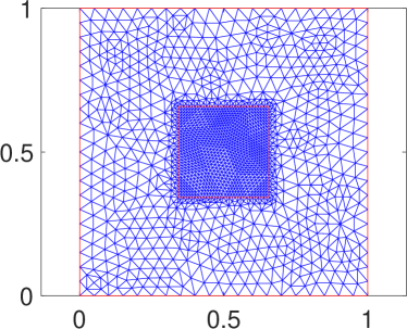
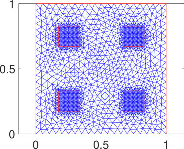
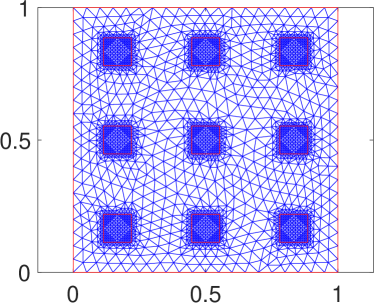
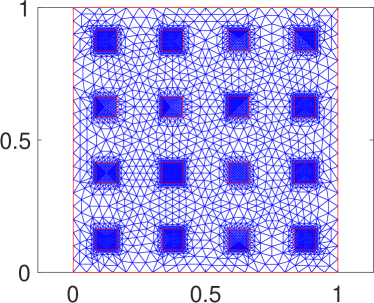
Figure 2. Location of the actuators. Cases $M_{\sigma}\in\{1,4,9,16\}$.

Example 4.1.

We take as initial states the constant functions

$$\widehat{y}_{0}(x)=\zeta_{2}\quad\mbox{and}\quad y_{0}(x)=\zeta_{3},$$

and we take the vanishing external force

$$h(t,x)=0.$$

Note that $\widehat{y}_{0}(x)$ is an unstable equilibrium and $y_{0}(x)$ is a stable equilibrium, for the free dynamics. Thus, our goal is to leave a stable state and to approach and stabilize an unstable one. In Fig. 3 we can see that the saturated feedback control is able to stabilize the error dynamics in case  $C_{u}\geq{\mathrm{e}}^{3.5}$.

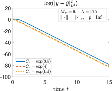
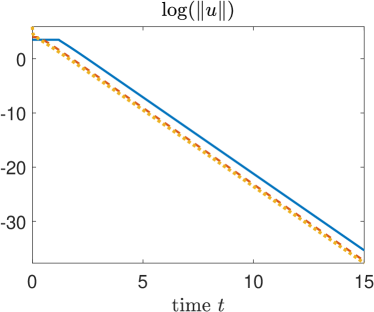
Figure 3. Norms of error and control. Large control constraint. (Ex. 4.1)

On the other hand, for magnitudes $C_{u}\leq{\mathrm{e}}^{1}$, in Fig. 4 we can see that the saturated control is not able to stabilize the error dynamics.

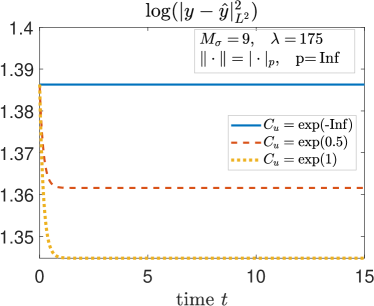
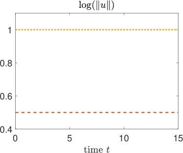
Figure 4. Norms of error and control. Small control constraint. (Ex. 4.1)

Example 4.2.

We compare the performance of the control generated by Algorithm 1 (RHC) with that of the explicitly given saturated control. For Algorithm  1, we set $T=1.25$ and $\delta=0.5$ and run the algorithm until the final computational time $T_{\infty}$ for two control cost parameters $\beta\in\{10^{-3},10^{-5}\}$. As initial states we take the constant functions

$$\widehat{y}_{0}(x)=\zeta_{3}\quad\mbox{and}\quad y_{0}(x)=\zeta_{1},$$

and as external force we take the time-periodic function

$$h(t,x)=\tfrac{1}{2}1_{\{s\geq 0\mid\left|\sin(6s)\right|_{{\mathbb{R}}}>\frac{1}{2}\}}(t)1_{\{w\in\Omega\mid\left|w\right|_{{\mathbb{R}}}^{2}<\frac{1}{2}\}}(x).$$ (4.1)

The initial states are stable equilibria of the free dynamics in the case of a vanishing external force, $h=0$. Here, we are taking a nonzero time-periodic external forcing, which induces the asymptotic periodic-like behavior shown in Fig. 5 for the norm of the targeted trajectory $\widehat{y}$. From Figs. 6–10, we can see that the saturated feedback control is able to stabilize the error dynamics for $C_{u}\geq{\mathrm{e}}^{1.5}$, whereas RHC is stabilizing for $C_{u}\geq{\mathrm{e}}^{1}$. This can be seen from Fig. 7, where the saturated control fails to track $\widehat{y}$, while RHC succeeds. For the case $C_{u}=e^{0.5}$, it can be seen in Fig. 6 that, none of the control laws is able to track $\widehat{y}$. As illustrated in Figs. 6–10, the saturated control is active for a longer interval compared to RHC. Further, observing the plots related to $\left|y-\widehat{y}\right|_{L^{2}((0,T_{\infty}),L^{2})}^{2}$, we can see that the influence of $\beta$ is only recognizable for $C_{u}\geq e^{2}$.

The value of the performance index function

$$J_{T_{\infty}}(u;0,y_{0},\widehat{y})=\left|y-\widehat{y}\right|_{L^{2}((0,T_{\infty}),L^{2})}^{2}+\beta\left|u\right|_{L^{2}((0,T_{\infty}),\mathbb{R}^{M_{\sigma}})}^{2},$$

for different control laws is reported in Table 1. As we would expect, in all the cases, RHC delivers better results than the saturated controls concerning the value of $J_{\infty}$. We can also see that as $C_{u}$ is getting larger the performance of the saturated control and RHC are getting closer to each other (except the case $C_{u}=e^{\infty}$).

	$(e^{0.5},25)$	$(e^{1},20)$	$(e^{1.5},10)$	$(e^{2},7)$	$(e^{\infty},5)$
RHC $\Bigl{.}\beta=10^{-3}\Bigr{.}$	$202.47$	$90.376$	$30.238$	$17.554$	$25.827$
SatCon $\lambda=175$	$203.04$	$152.93$	$34.226$	$17.922$	$30.787$
RHC $\Bigl{.}\beta=10^{-5}\Bigr{.}$	$201.86$	$89.497$	$29.415$	$15.459$	1.0466
SatCon $\lambda=175$	$202.47$	$151.73$	$33.439$	$16.729$	$1.0973$

Table 1. The value of $J_{T_{\infty}}$. (Ex. 4.2)

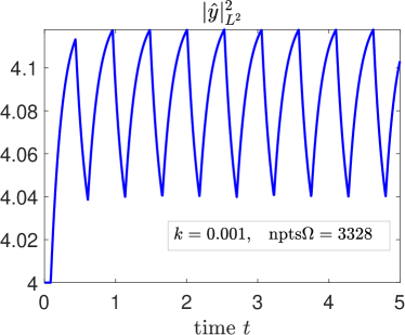
Figure 5. Norm of targeted trajectory. (Ex. 4.2)

Note that for large time the logarithm of the norm of the error $y-\widehat{y}$ stays close to a small value, approximately around $-35$. This can be explained due to the accuracy/precision used in the numerical computations, in fact that value is relatively close to the standard Matlab precision ${\tt eps}\approx 10^{-16}$ we have used; indeed ${\mathrm{e}}^{-35}\approx 6\times 10^{-16}$.

Recall that we are also computing the targeted trajectory $\widehat{y}$, whose values are then used to compute the controlled trajectory $y$. We cannot expect that the computational errors associated with the solution of the two systems will cancel each other. Hence, the aforementioned behavior for the norm of $y-\widehat{y}$ is consistent.

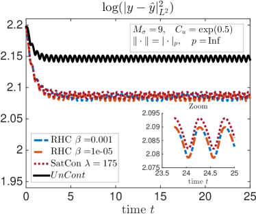
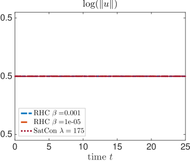
Figure 6. Norms of error and control for $(C_{u},T_{\infty})=(e^{0.5},25)$. (Ex. 4.2)

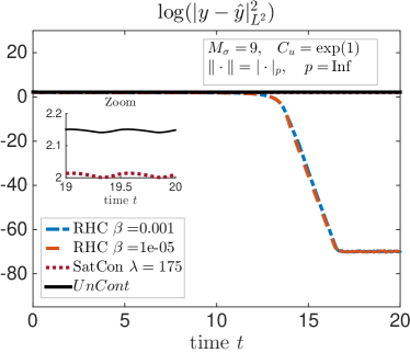
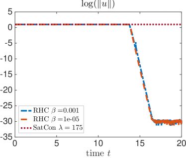
Figure 7. Norms of error and control for $(C_{u},T_{\infty})=(e^{1},20)$. (Ex. 4.2)

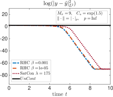
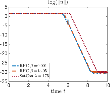
Figure 8. Norms of error and control. $(C_{u},T_{\infty})=(e^{1.5},10)$. (Ex. 4.2)

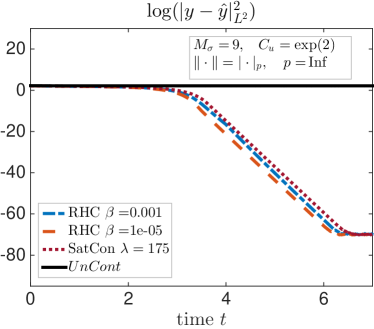
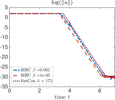
Figure 9. Norms of error and control. $(C_{u},T_{\infty})=(e^{2},7)$. (Ex. 4.2)

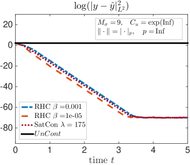
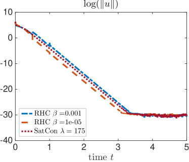
Figure 10. Norms of error and control. $(C_{u},T_{\infty})=(e^{\infty},5)$. (Ex. 4.2)

Example 4.3.

Now we take as initial conditions

$$\widehat{y}_{0}(x)=10-20x_{1}x_{2};\qquad y_{0}(x)=-10x_{1}+x_{2}.$$

Their norms as well as the norm of the initial error $z_{0}=y_{0}-\widehat{y}_{0}$ are large when compared to those in Examples 4.1 and 4.2. The external forcing is taken as (4.1). In Fig. 11, we can see that the norm of the targeted trajectory $\widehat{y}$ decreases fast as long as it is large (cf. Sect. 2.3). Asymptotically it exhibits again a periodic-like behavior near $2$.

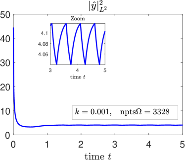
Figure 11. Norm of targeted trajectory. (Ex. 4.3)

Comparing Figs. 12 and 13, we see again that we achieve the stability of the controlled error dynamics if, and only if, the magnitude $C_{u}$ of the control constraint is large enough.

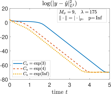
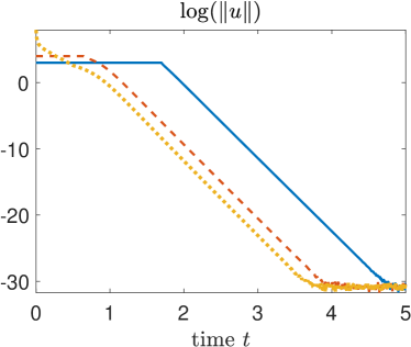
Figure 12. Norms of error and control. Large control constraint. (Ex. 4.3)

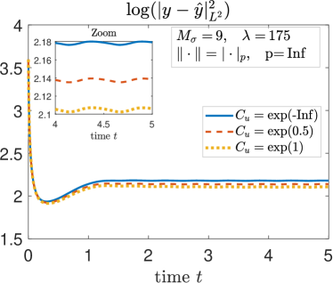
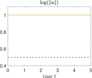
Figure 13. Norms of error and control. Small control constraint. (Ex. 4.3)

Example 4.4.

We take the initial states and external force again as in Example 4.3. But, instead of investigating the role played by the control constraint $C_{u}$, we focus on parameters $M$ and $\lambda$ determining the feedback law.In Fig. 12 we see that by increasing the control constraint $C_{u}$ we approach the behavior of the unconstrained limit case $C_{u}=+\infty$. To verify that an arbitrary exponential decrease rate $\mu$ can be achieved with a sufficiently large $C_{u}=C_{u}(\mu)$, it is enough to show that this rate can be achieved with the unconstrained feedback. Indeed, in Fig. 14 we confirm that by increasing $M$ and $\lambda$ we reach larger exponential decrease rates. This is consistent with our theoretical result which says that we can achieve an arbitrary large exponential decrease rate $\mu$. We recall the idea of the proof: for small time the exponential decrease rate is guaranteed for large initial errors, with norm larger than a suitable constant $D=D(\mu)$; for such $D$ we choose $M$ and $\lambda$ large enough to achieve such exponential decrease rate with the unconstrained control; finally we choose $C_{u}=C_{u}(D(\mu))$ large enough so that the constraint is inactive for an error norm smaller than $D$.

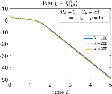
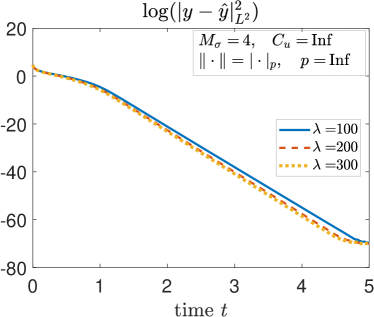
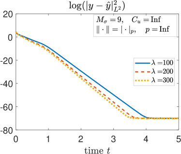
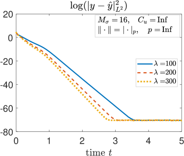
Figure 14. Norm of error for several pairs $(M_{\sigma},\lambda)$. $C_{u}=+\infty$. (Ex. 4.4)

Remark 4.5.

In Fig. 14 we see that with a single actuator, $M_{\sigma}=1$, we are able to achieve the exponential stability of the error dynamics, for a suitable rate $\mu_{1}$. This does not follow from, nor contradicts, our theoretical results, from which we have that exponential stability with an apriori given rate $\mu$ holds for large enough $M_{\sigma}$. This leads us to the following question: (when, if possible) can we guarantee/achieve exponential stability with a single actuator? This could be an interesting problem for future research.

Above, we have taken $\lambda\geq 100$, which allow us to obtain large exponential decrease rates for the error norm. Fig. 15 shows that, for  $M_{\sigma}=16$ actuators, we can achieve exponential stability of the error dynamics with $\lambda\geq 5$. However, the figure also shows that $\lambda$ cannot be taken arbitrarily small, since the error dynamics is not exponentially stable with $\lambda\leq 1$.

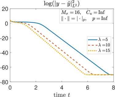
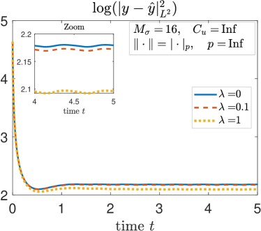
Figure 15. Norm of error for small $\lambda$. $C_{u}=+\infty$. (Ex. 4.5)

5. Concluding remarks

We have shown the global stabilizability to trajectories for the Schlögl model for chemical reactions, with a finite number of internal actuators and under control magnitude constraints. The number of actuators and the magnitude of the controls depend on the diffusion coefficient and on the nonlinearity, but they are independent of the external forcing and the targeted trajectory. The stabilizing controls can be taken as the saturation of an explicit feedback operator. Its performance was compared to a receding horizon control approach.

An interesting topic for future work could the investigation of systems coupling the Schlögl parabolic equation with an ODE. These are systems of FitzHugh–Nagumo type modeling phenomena in neurology and electrophysiology.

Appendix

A.1. Proof of Theorem 1.5

Let $\mu>0$. Taking the feedback control $u_{1}=(r-2\mu)z$ and multiplying the dynamics in (1.8) by $2z$, we find that $\tfrac{{\mathrm{d}}}{{\mathrm{d}}t}z^{2}=-2\mu z^{2}$, from which we obtain $z^{2}(t)={\mathrm{e}}^{-2\mu(t-s)}z^{2}(s)$. ∎

A.2. Proof of Theorem 1.6

Let $r<0$. Let us fix an arbitrary $C_{u}\in{\mathbb{R}}_{+}$ and an arbitrary control input function $u=u_{1}$ satisfying $\left|u(t)\right|_{{\mathbb{R}}}\leq C_{u}$, for all $t\geq 0$. Multiplying the dynamics in (1.8) by $2z$, we find that

$$\tfrac{{\mathrm{d}}}{{\mathrm{d}}t}z^{2} =-2rz^{2}+2u_{1}z\geq-2rz^{2}-2C_{u}\left|z\right|_{{\mathbb{R}}}$$

$$=2\left|z\right|_{{\mathbb{R}}}(-r\left|z\right|_{{\mathbb{R}}}-C_{u}),$$

which implies that

$$\tfrac{{\mathrm{d}}}{{\mathrm{d}}t}z^{2}(t)>0\quad\mbox{if}\quad\left|z(t)\right|_{{\mathbb{R}}}>\tfrac{C_{u}}{-r}.$$

Thus, if $\left|z(0)\right|_{{\mathbb{R}}}>\tfrac{C_{u}}{-r}$ then $\left|z(t)\right|_{{\mathbb{R}}}>\left|z(0)\right|_{{\mathbb{R}}}$ for all $t>0$. ∎

Acknowledgments: K. K. and S. R. were supported by ERC advanced grant 668998 (OCLOC) under the EU’s H2020 research program. S. R. also acknowledges partial support from Austrian Science Fund (FWF): P 33432-NBL.

References

• [1] B. Azmi and K. Kunisch. A hybrid finite-dimensional RHC for stabilization of time-varying parabolic equations. SIAM J. Control Optim., 57(5):3496–3526, 2019. doi:10.1137/19M1239787.
• [2] B. Azmi and K. Kunisch. Analysis of the Barzilai–Borwein step-sizes for problems in Hilbert spaces. J. Optim. Theory Appl., 185(3):819–844, 2020. doi:10.1007/s10957-020-01677-y.
• [3] B. Azmi and K. Kunisch. On the convergence and mesh-independent property of the Barzilai–Borwein method for PDE-constrained optimization. IMA J. Numer. Anal., 2021. drab056. doi:10.1093/imanum/drab056.
• [4] A. Azouani and E. S. Titi. Feedback control of nonlinear dissipative systems by finite determining parameters – a reaction-diffusion paradigm. Evol. Equ. Control Theory, 3(4):579–594, 2014. doi:10.3934/eect.2014.3.579.
• [5] M. Badra and T. Takahashi. Stabilization of parabolic nonlinear systems with finite dimensional feedback or dynamical controllers: Application to the Navier–Stokes system. SIAM J. Control Optim., 49(2):420–463, 2011. doi:10.1137/090778146.
• [6] A. Balogh and M. Krstic. Burgers’ equation with nonlinear boundary feedback: $H^{1}$ stability, well-posedness and simulation. Math. Probl. Engineering, 6:189–200, 2000. doi:10.1155/S1024123X00001320.
• [7] C. Barbu, J. J. Cheng, and R. A. Freeman. Achieving maximum regions of attraction for unstable linear systems with control constraints. In Proceedings of the American Control Conference (ACC), Albuquerque, New Mexico, pages 848–852, 1997. doi:10.1109/ACC.1997.611924.
• [8] V. Barbu. Stabilization of Navier–Stokes Flows. Comm. Control Engrg. Ser. Springer-Verlag London, 2011. doi:10.1007/978-0-85729-043-4.
• [9] V. Barbu. Stabilization of Navier–Stokes equations by oblique boundary feedback controllers. SIAM J. Control Optim., 50(4):2288–2307, 2012. doi:10.1137/110837164.
• [10] V. Barbu. Boundary stabilization of equilibrium solutions to parabolic equations. IEEE Trans. Automat. Control, 58(9):2416–2420, 2013. doi:10.1109/TAC.2013.2254013.
• [11] V. Barbu, I. Lasiecka, and R. Triggiani. Abstract settings for tangential boundary stabilization of Navier–Stokes equations by high- and low-gain feedback controllers. Nonlinear Anal., 64(12):2704–2746, 2006. doi:10.1016/j.na.2005.09.012.
• [12] V. Barbu, S. S. Rodrigues, and A. Shirikyan. Internal exponential stabilization to a nonstationary solution for 3D Navier–Stokes equations. SIAM J. Control Optim., 49(4):1454–1478, 2011. doi:10.1137/100785739.
• [13] V. Barbu and R. Triggiani. Internal stabilization of Navier–Stokes equations with finite-dimensional controllers. Indiana Univ. Math. J., 53(5):1443–1494, 2004. doi:10.1512/iumj.2004.53.2445.
• [14] J. Barzilai and J. M. Borwein. Two-point step size gradient methods. IMA J. Numer. Anal., 8(1):141–148, 1988. doi:10.1093/imanum/8.1.141.
• [15] J. Bey. Simplicial grid refinement: on Freudenthal algorithm and the optimal number of congruence classes. Numer. Math., 85:1–29, 2000. doi:10.1007/s002110000108.
• [16] T. Breiten, K. Kunisch, and S. S. Rodrigues. Feedback stabilization to nonstationary solutions of a class of reaction diffusion equations of FitzHugh–Nagumo type. SIAM J. Control Optim., 55(4):2684–2713, 2017. doi:10.1137/15M1038165.
• [17] J. Cochran, R. Vazquez, and M. Krstic. Backstepping boundary control of Navier–Stokes channel flow: A 3D extension. In Proceedings of the 2006 American Control Conference, Minneapolis, Minnesota, USA, pages 769–774, 6 2006. URL: 10.1109/ACC.2006.1655449.
• [18] M.L. Corradini, A. Cristofaro, and G. Orlando. Robust stabilization of multi input plants with saturating actuators. IEEE Trans. Automat. Control, 55(2):419–425, 2010. doi:10.1109/TAC.2009.2036308.
• [19] J. Deutscher. Backstepping design of robust output feedback regulators for boundary controlled parabolic PDEs. IEEE Trans. Automat. Control, 61(8):2288–2294, 2016. doi:10.1109/TAC.2015.2491718.
• [20] H. Edelsbrunner and D. R. Grayson. Edgewise subdivision of a simplex. Discrete Comput. Geom., 24:707–719, 2000. doi:10.1007/s004540010063.
• [21] R. FitzHugh. Impulses and physiological states in theoretical models of nerve membrane. Biophysical J., 1(6):445–466, 1937. doi:doi:10.1016/S0006-3495(61)86902-6.
• [22] M. Gugat and F. Troeltzsch. Boundary feedback stabilization of the schlögl system. Automatica J. IFAC, 51:192–1199, 2015. doi:10.1016/j.automatica.2014.10.106.
• [23] T. Hu, Z. Lin, and L. Qiu. Stabilization of exponentially unstable linear systems with saturating actuators. IEEE Trans. Automat. Control, 46(6):973–979, 2001. doi:10.1109/9.928610.
• [24] M. Krstic, L. Magnis, and R. Vazquez. Nonlinear control of the viscous Burgers equation: Trajectory generation, tracking, and observer design. J. Dyn. Syst. Meas. Control, 131(2):{021012}, 2009. doi:10.1115/1.3023128.
• [25] K. Kunisch and S. S. Rodrigues. Explicit exponential stabilization of nonautonomous linear parabolic-like systems by a finite number of internal actuators. ESAIM Control Optim. Calc. Var., 25:{67}, 2019. doi:10.1051/cocv/2018054.
• [26] K. Kunisch and S. S. Rodrigues. Oblique projection based stabilizing feedback for nonautonomous coupled parabolic-ode systems. Discrete Contin. Dyn. Syst., 39(11):6355–6389, 2019. doi:10.3934/dcds.2019276.
• [27] K. Kunisch, S. S. Rodrigues, and D. Walter. Learning an optimal feedback operator semiglobally stabilizing semilinear parabolic equations. Appl. Math. Optim., 2021. doi:10.1007/s00245-021-09769-5.
• [28] I. Lasiecka and T. I. Seidman. Strong stability of elastic control systems with dissipative saturating feedback. Systems Control Lett., 48(3-4):243–252, 2003. doi:10.1016/S0167-6911(02)00269-4.
• [29] T. Lauvdal and T.I. Fossen. Stabilization of linear unstable systems with control constraints. In Proceedings of the 36th IEEE Conference on Decision and Control, pages 4504–4509, 1997. doi:10.1109/CDC.1997.649680.
• [30] W. Liu, Y. Chitour, and E. Sontag. On finite-gain stabilizability of linear systems subject to input saturation. SIAM J. Control Optim., 34(4):1190–1219, 1996. doi:10.1137/S0363012994263469.
• [31] E. Lunasin and E.S. Titi. Finite determining parameters feedback control for distributed nonlinear dissipative systems – a computational study. Evol. Equ. Control Theory, 6(4):535–557, 2017. doi:10.3934/eect.2017027.
• [32] A. Mironchenko, C. Prieur, and F. Wirth. Local stabilization of an unstable parabolic equation via saturated controls. IEEE Trans. Automat. Control, 66(5):2162–2176, 2021. doi:10.1109/TAC.2020.3007733.
• [33] J. Nagumo, S. Arimoto, and S. Yoshizawa. An active pulse transmission line simulating nerve axon. In Proc. of the IRE, pages 2061–2070, October 1962. doi:10.1109/JRPROC.1962.288235.
• [34] D. Phan and S.S. Rodrigues. Stabilization to trajectories for parabolic equations. Math. Control Signals Syst., 30(2):{11}, 2018. doi:10.1007/s00498-018-0218-0.
• [35] C. Prieur and E. Trélat. Feedback stabilization of a 1-d linear reaction–diffusion equation with delay boundary control. IEEE Trans. Automat. Control, 64(4):1415–1425, 2019. doi:10.1109/TAC.2018.2849560.
• [36] J.-P. Raymond. Stabilizability of infinite-dimensional systems by finite-dimensional controls. Comput. Methods Appl. Math., 19(4):797–811, 2019. doi:10.1515/cmam-2018-0031.
• [37] S.S. Rodrigues. Feedback boundary stabilization to trajectories for 3D Navier–Stokes equations. Appl. Math. Optim., 2018. doi:10.1007/s00245-017-9474-5.
• [38] S.S. Rodrigues. Semiglobal exponential stabilization of nonautonomous semilinear parabolic-like systems. Evol. Equ. Control Theory, 9(3):635–672, 2020. doi:10.3934/eect.2020027.
• [39] S.S. Rodrigues. Oblique projection exponential dynamical observer for nonautonomous linear parabolic-like equations. SIAM J. Control Optim., 59(1):464–488, 2021. doi:10.1137/19M1278934.
• [40] S.S. Rodrigues. Oblique projection output-based feedback stabilization of nonautonomous parabolic equations. Automatica J. IFAC, 129:{109621}, 2021. doi:10.1016/j.automatica.2021.109621.
• [41] S.S. Rodrigues. Semiglobal oblique projection exponential dynamical observers for nonautonomous semilinear parabolic-like equations. J. Nonlin. Sci., 31(6):{100}, 2021. doi:10.1007/s00332-021-09756-8.
• [42] A. Saberi, Z. Lin, and A.R. Teel. Control of linear systems with saturating actuators. IEEE Trans. Automat. Control, 41(3):368–378, 1996. doi:10.1109/9.486638.
• [43] F. Schlögl. Chemical reaction models for non-equilibrium phase transitions. Z. Physik, 253:147–161, 1972. doi:10.1007/BF01379769.
• [44] T.I. Seidman and H. Li. A note on stabilization with saturating feedback. Discrete Contin. Dyn. Syst., 7(2):319–328, 2001. doi:10.3934/dcds.2001.7.319.
• [45] M. Slemrod. Feedback stabilization of a linear control system in Hilbert space with an a priori bounded control. Math. Control Signals Syst., 2(3):265–285, 1989. doi:10.1007/BF02551387.
• [46] H.J. Sussmann, E.D. Sontag, and Y. Yang. A general result on the stabilization of linear systems using bounded controls. IEEE Trans. Automat. Control, 39(12):2411–2425, 1994. doi:10.1109/9.362853.
• [47] A.R. Teel. Global stabilization and restricted tracking for multiple integrators with bounded controls. Systems Control Lett., 18(3):165–171, 1992. doi:10.1016/0167-6911(92)90001-9.
• [48] G.F. Wredenhagen and P.R. Bélanger. Piecewise-linear LQ control for systems with input constraints. Automatica J. IFAC, 30(3):403–416, 1994. doi:10.1016/0005-1098(94)90118-X.
• [49] B. Zhou and J. Lam. Global stabilization of linearized spacecraft rendezvous system by saturated linear feedback. IEEE Trans. Control Syst. Tech., 25(6):2185–2193, 2017. doi:10.1109/TCST.2016.2632529.