BayesDLMfMRI: Bayesian Matrix-Variate Dynamic Linear Models for Task-based fRMI Modeling in R

Abstract

This article introduces an R package to perform statistical analysis for task-based fMRI data at both individual and group levels. The analysis to detect brain activation at the individual level is based on modeling the fMRI signal using Matrix-Variate Dynamic Linear Models (MDLM). Therefore, the analysis for the group stage is based on posterior distributions of the state parameter obtained from the modeling at the individual level. In this way, this package offers several R functions with different algorithms to perform inference on the state parameter to assess brain activation for both individual and group stages. Those functions allow for parallel computation when the analysis is performed for the entire brain as well as analysis at specific voxels when it is required.

Keywords First keyword  $\cdot$ Second keyword  $\cdot$ More

1 Introduction: fMRI packages with options for Bayesian Analysis

Statistical modeling of processed fMRI data is a challenging problem, which has caught the attention of the statistical community in the past two decades. Large amount of observations are usually obtained with only one subject in an fMRI session which makes the implementation of more appropriate and sophisticated statistical models that can account for the spatiotemporal structures that are usually present in this type of data really challenging. From a Bayesian perspective, there have been published and proposed different types of models to model fMRI data (see for instance Zhang et al. (2016), Eklund et al. (2017), Bezener et al. (2018), Yu et al. (2018) and a complete review by Zhang et al. (2015)). Despite that, just a few software implementations of Bayesian methods are available for fMRI data analysis. For instance, the FSL software (Jenkinson et al., 2012) offers a Bayesian procedure for the group stage analysis, which depends on a Frequentist or Classical output from the individual stage. Another popular software among practioners in the neurosicience community with implementations of Bayesian methods is the SPM package (Penny et al., 2011). It has alternatives for Bayesian analysis to both individual and group stages, but as in the case of the FSL package, the group analysis depends on a Frequentist individaul stage output. There is also available a MATLAB GUI called NPBayes-fMRI (Kook et al., 2019), which is an implementation of the work proposed by Zhang et al. (2016), a fully Bayesian modeling for individual and group stages. In R (R Core Team, 2018), tools for different types of fMRI data analysis are provided in packages like fmri (Tabelow and Polzehl, 2011), oro.nifti (Whitcher et al., 2011), neurobase (Muschelli, 2018), and neuRosim (Welvaert et al., 2011). For fMRI data analysis under a Bayesian approach there was a package called cudaBayesreg (da Silva et al., 2011), which was removed recently from the CRAN repository. Thus, the package BHMSMAfMRI (Sanyal and Ferreira, 2019) is to our knowledge the only Bayesian option for fMRI data analysis in R to this date.

In this work, we are presenting an R package called BayesDLMfMRI, which is an implementation of the method proposed in Jiménez et al. (2019) and Jiménez (2019). The BayesDLMfMRI permits to perform fMRI individual and group analysis based on the Matrix-Variate Dynamic Linear Model (MVDLM) proposed by Quintana (1985). Given this type of analysis usually involved large amounts of data, we take advantage of the packages Rcpp (Eddelbuettel et al., 2011) and RcppArmadillo (Eddelbuettel and Sanderson, 2014) in order to speed up the computation time. BayesDLMfMRI also depends internally on the package pbapply (Solymos and Zawadzki, 2019), which allows the user to visualize a progress bar while the process is run in either sequence or parallel. In order to run an analysis using our package the user must provide a 4D array (or a 4D$\times N$ array for a group analysis with $N$ subjects) containing the sequence of processed images and a design matrix whose columns are related to the so-called expected blood-oxygen-Level dependent (BOLD) response and/or some other covariates related to particular subjects’ characteristics. To process the raw images, we recommend the use of packages such as FSL or SPM. And to build the expected BOLD response the user has options like the fmri package, which allows defining different types of models to represent the haemodynamic response function (HRF). BayesDLMfMRI package is intended to be just another well tested and assessed tool for the practitioners who are interested to perform statistical analysis of processed fMRI images from a Bayesian perspective. In the next section, we give a brief description of the model and methods on which the BayesDLMfMRI package is based and present its R functions to perform fMRI data analysis. In section three, we present some examples to illustrate the use of the package and in the final section, we give some concluding remarks.

2 Methods and software

Table 1: Functions implemented in the BayesDLMfMRI package for fMRI (group) individual analysis. LLT stands for Transformation Linear Test, which is the same as the average cluster effect (ACE) distribution defined in ArchiveRef.

Function	Description
(ffdGroupEvidenceFEST) ffdEvidenceFEST	It returns 3D arrays to build (group) individual activation evidence maps (based on outputs from MVDLM) fitting an MVDLM at individual level and using the FEST algorithm to assess voxel activation. There are two options related to the posterior distribution of $\Theta_{\scaleto{[i,j,k]t\mathstrut}{4pt}}^{\scaleto{(z)\mathstrut}{4pt}}$: LLT and Joint. Each one runs independently and must be set by the user as an input parameter.
(ffdGroupEvidenceFFBS) ffdEvidenceFFBS	It returns 3D arrays to build (group) individual activation evidence maps (based on outputs from MVDLM) fitting an MVDLM and using the FFBS algorithm to assess voxel activation. The options LLT and Joint related to the posterior distribution of $\Theta_{\scaleto{[i,j,k]t\mathstrut}{4pt}}^{\scaleto{(z)\mathstrut}{4pt}}$ are simultaneously executed in the same run.
(ffdGroupEvidenceFSTS) ffdEvidenceFSTS	Same features as (ffdGroupEvidenceFFBS) ffdEvidenceFFBS, though using the FSTS algorithm.
(GroupSingleVoxelFEST) SingleVoxelFEST	Produces some usefull outputs from a single voxel analysis related to the FEST algorithm
(GroupSingleVoxelFFBS) SingleVoxelFFBS	Same features as (GroupSingleVoxelFEST) SingleVoxelFEST, though using the FFBS algorithm
(GroupSingleVoxelFSTS) SingleVoxelFSTS	Same features as (GroupSingleVoxelFEST) SingleVoxelFEST, though using the FSTS algorithm

The type of MVDLM which this package relies on is the version originally developed by Quintana (1985) and Quintana (1987). Here, we just give a brief description of the model and methods. For a better understanding of the method implemented in this package for the individual stage, see Jiménez et al. (2019). Let $\mathbf{Y}_{\scaleto{[i,j,k]t\mathstrut}{6pt}}^{(z)}$ be a $q\times 1$ random vector representing the cluster of observed BOLD responses at position $(i,j,k)$ in the brain image, time $t$ and subject $z$, for $i=1,\ldots,d_{1}$, $j=1,\ldots,d_{2}$, $k=1,\ldots,d_{3}$, $t=1,\ldots,T$ and $z=1\ldots,N$. Thus, the cluster of BOLD signals is modeled as

$$\begin{array}[]{lccl}\text{Observation:}&\mathbf{Y}_{\scaleto{[i,j,k]t\mathstrut}{4pt}}^{\scaleto{(z)\mathstrut}{4pt}}&=&\mathbf{F}^{{}^{\prime}}_{t}\Theta_{\scaleto{[i,j,k]t\mathstrut}{4pt}}^{\scaleto{(z)\mathstrut}{4pt}}+\bm{\nu}_{\scaleto{[i,j,k]t\mathstrut}{4pt}}^{\scaleto{{}^{\prime}(z)\mathstrut}{4pt}}\\ \text{Evolution:}&\Theta_{\scaleto{[i,j,k]t\mathstrut}{4pt}}^{\scaleto{(z)\mathstrut}{4pt}}&=&\mathbf{G}_{t}\Theta_{\scaleto{[i,j,k]t-1\mathstrut}{4pt}}^{\scaleto{(z)\mathstrut}{4pt}}+\Omega_{\scaleto{[i,j,k]t\mathstrut}{4pt}}^{\scaleto{(z)\mathstrut}{4pt}},\\ \end{array}$$ (1)

where, for each $t$ we have a $q\times 1$ vector $\bm{\nu}_{\scaleto{[i,j,k]t\mathstrut}{4pt}}^{\scaleto{{}^{\prime}(z)\mathstrut}{4pt}}$ of observational errors, a $p\times q$ matrix $\Theta_{\scaleto{[i,j,k]t\mathstrut}{4pt}}$ of state parameters, a $p\times q$ matrix $\Omega_{\scaleto{[i,j,k]t\mathstrut}{4pt}}^{\scaleto{(z)\mathstrut}{4pt}}$ of evolution errors. The $1\times p$ and $p\times p$ matrices $\mathbf{F}^{{}^{\prime}}_{t}$ and $\mathbf{G}_{t}$ respectivelly are common to each of the $q$ univariate DLMs. The covariates related to the design being used, either a block or an event-related design as well as other characteristics of the subjects, can be included in the columns of $\mathbf{F}^{{}^{\prime}}_{t}$. For individual analysis the model (1) is fitted to every cluster of voxels related to position $[i,j,k]$ in the brain image and the cluster size depends on the $r$ distance, which is a parameter defined by the user. To identify wether or not there is significant evidence of cluster activation or brain reaction at region $[i,j,k]$, three different algorithms (FEST, FSTS and FFBS) proposed in Jiménez et al. (2019) are implemented. Those algorithms are sampling schemes that allow to draw on-line trajectory curves related to the state parameter $\Theta_{\scaleto{[i,j,k]t\mathstrut}{4pt}}^{\scaleto{(z)\mathstrut}{4pt}}$, and with those resulting samples a Monte Carlo evidence related to the event of cluster activation is computed. The information obtained from the first stage can be combined in different ways to produce several measures of evidence for the group activation. For a better understanding of the method implemented in this package for the group stage, see Jiménez (2019). In table 2, the package’s functions for (group) individual analysis and a brief description of them are presented.

3 Illustrations

In order to show some practical illustrations about the use of the BayesDLMfMRI package, we use data related to an fMRI experiment where a sound stimilus is presented. That experiment is intended to offer a "voice localizer" scan, which allows rapid and reliable localization of the voice-sensitive "temporal voice areas" (TVA) of human auditory cortex (Pernet et al., 2015). The data of this "voice localizer" scan is freely available on the online platform OpenNEURO (Gorgolewski et al., 2017). In the original experiment, the voice and non-voice sounds are separately analyzed, but here we merge both sounds in one block as it were just one stimulus (see figure 1). For the individual analysis, we select one from the 217 subjects whose data are available on OpenNEURO, specifically, we take the data from sub-007. To illustrate the use of the group analysis functions, we take 20 subjects (sub-001:sub-021). The raw fMRI data is preprocessed using the standard processing pipelines implemented on the FSL software for motion correction, spatial smoothing and other necessary procedures to perform statistical analysis for both individual and group stages.

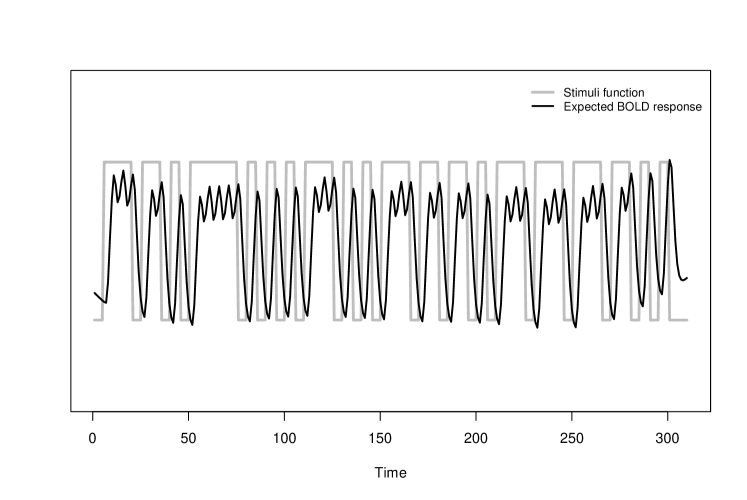
Figure 1: Merged stimuli function for voice and non-voice sounds with its respective expected BOLD response function for the "voice localizer" example.

Individual analysis

In order to run any of the functions related to individual analysis, the user must provide two inputs: an array of four dimensions containing the MRI images and a matrix whose columns contain the covariates to model the observed BOLD response. Thus, we read the data.nii.qz file, which contains the MRI images, using the function readNIFTI from the package oro.nifti and the covariates.cvs file which contains the expected BOLD response (show in figure 1) and its derivative respectively.

R> library("oro.nifti")R> fMRI.data <- readNIfTI("./fMRIData/sub-007.nii.gz", reorient=FALSE)R> fMRI.data <- fMRI.data@.DataR> dim(fMRI.data)

[1]  91 109  91 310

R> Covariates <- read.csv("./covariates.csv", header=FALSE, sep="")R> dim(Covariates)

[1] 310   2

To perform a voxel-wise anaylsis to obtain a 3D array with measurements of activation evidence for every voxel, the user has three options (ffdEvidenceFEST, ffdEvidenceFFBS and ffdEvidenceFSTS), which at the same time can yield three different types of evidence measurements for voxel activation. Just to ilustrate their use, we run them using the "voice localizer" example.

R> library(devtools)R> install_github("JohnatanLAB/BayesDLMfMRI")R> library(BayesDLMfMRI)R> res <- ffdEvidenceFEST(ffdc = fMRI.data, covariates = Covariates,+ m0 = 0, Cova = 100, delta = 0.95, S0 = 1, n0 = 1, Nsimu1 = 100, Cutpos1 = 30,+ r1 = 1, Test = "LTT",  Ncores = 15)

  |++++++++++++++++++++++++++++++++++++++++++++++++++| 100% elapsed = 05m 36s

The arguments m0, Cova, S0 and n0 are the hyper-parameters related to the joint prior distribution of $(\Theta_{\scaleto{[i,j,k]t\mathstrut}{4pt}}^{\scaleto{(z)\mathstrut}{4pt}},\Sigma_{\scaleto{[i,j,k]t\mathstrut}{4pt}}^{\scaleto{(z)\mathstrut}{4pt}})$. For this example, we are setting a "vague" prior distribution acording to Quintana and West (1987), where m0 = 0 define a null matrix with zero values in all its entries and both Cova = 100 and S0 = 1 define diagonal matrices. r1 is the euclidean distance, which defines the size of the cluster of voxels jointly modeled. Test is the parameter related to the test selected by the user, for which there are two options: "LTT" and "Joint". "Ncores" is the argument related to the number of cores when the process is executed in parallel. Nsimu1 is the number of simulated on-line trajectories related to the state parameter $\Theta_{\scaleto{[i,j,k]t\mathstrut}{4pt}}^{\scaleto{(z)\mathstrut}{4pt}}$. From our own experience dealing with different sets of fMRI data, we recommend Nsimu1 = 100 as a good number of draws to obtain reliable results. Cutpos1 is the time up from where the on-line trajectories are considered in order to compute the activation evidence and delta is the value of the discount factor. For a better understanding about the setting of these two last arguments, see (Archive1).

R> str(res)

List of 2 $ : num [1:91, 1:109, 1:91] 0 0 0 0 0 0 0 0 0 0 ... $ : num [1:91, 1:109, 1:91] 0 0 0 0 0 0 0 0 0 0 ...

R> dim(res[[1]])

[1]  91 109  91

The output for the ffdEvidenceFEST function depends on the type of Test set by the user. For Test = "LTT" the function returns a list of the type res[[p]][x, y, z], where [[p]] represents the column position in the covariates matrix and [x, y, z] represent the voxel position in the brain image. Thus, for the "voice localizer" example res[[1]] and res[[2]] are the 3D arrays related to the evidence for brain activation related to the BOLD response for the auditory stimuli and its derivative respectively. When Test = Joint the output returned is an array

R> library(neurobase)R> res.auxi <- res[[1]]R> ffd <- readNIfTI("./standard.nii.gz")R> Z.visual.c <- nifti(res.auxi, datatype=16)R> ortho2(ffd, ifelse(Z.visual.c > 0.95, Z.visual.c, NA),+  col.y = heat.colors(50), ycolorbar = TRUE, ybreaks = seq(0.95, 1, by = 0.001))

The neurobase package is one amongst several options available in R to visualize MRI images. In this example, we use its ortho2() function in order to plot the evidence activation map. The standar.nii.gz contains the MNI brain atlas, which is used in this work as a reference space for individual and group analysis. For a better understanding of the use of brain atlas, see Brett et al. (2002).

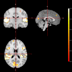
Figure 2: Activations maps obtained with the functions ffdEvidenceFEST (left) and ffdEvidenceFFBS (right) using the "Joint" as sampler distribution.

R> res <- ffdEvidenceFEST(ffdc = fMRI.data, covariates = Covariates,+  m0 = 0, Cova = 100, delta = 0.95, S0 = 1, n0 = 1, Nsimu1 = 100, Cutpos1 = 30,+  r1 = 2, Test = "JointTest",  Ncores = 15)

 |++++++++++++++++++++++++++++++++++++++++++++++++++| 100% elapsed = 28m 57s

R> str(res)

List of 4 $ : num [1:91, 1:109, 1:91] 0 0 0 0 0 0 0 0 0 0 ... $ : num [1:91, 1:109, 1:91] 0 0 0 0 0 0 0 0 0 0 ... $ : num [1:91, 1:109, 1:91] 0 0 0 0 0 0 0 0 0 0 ...

For both ffdEvidenceFFBS and ffdEvidenceFSTS the input arguments and output structures are the same. Below we run the "voice localizer" example using the ffdEvidenceFFBS function. It returns a list of the form res[[T]][p,x,y,z], where T defines the type of test (T = 1 for "Marginal", T = 2 for "JointTest", and T = 3 for "LTT"), p represents the column position in the covariates matrix and x, y, z represent the voxel position in the brain image.

#Change JointTest for JointR> res <- ffdEvidenceFFBS(ffdc = fMRI.data, covariates = covariables, m0 = 0,+  Cova = 100, delta = 0.95, S0 = 1,n0 = 1, Nsimu1 = 100, Cutpos1 = 30,+  r1 = 1,  Ncores = 15)

 |++++++++++++++++++++++++++++++++++++++++++++++++++| 100% elapsed = 19m 08s

R> str(res)

List of 3 $ : num [1:2, 1:91, 1:109, 1:91] 0 0 0 0 0 0 0 0 0 0 ... $ : num [1:2, 1:91, 1:109, 1:91] 0 0 0 0 0 0 0 0 0 0 ... $ : num [1:2, 1:91, 1:109, 1:91] 0 0 0 0 0 0 0 0 0 0 ...$

R> library(neurobase)R> res.auxi <- res[[3]][1,,,]R> ffd <- readNIfTI("standard.nii.gz")R> Z.visual.c <- nifti(res.auxi, datatype=16)R> ortho2(ffd, ifelse(Z.visual.c > 0.95, Z.visual.c, NA),+  col.y = heat.colors(50), ycolorbar = TRUE, ybreaks = seq(0.95, 1, by = 0.001))

The BayesDLMfMRI package also has functions that allow taking a closer look for specific voxels defined by the user. For instance, let’s suppose we are interested to see some of the output elements related to the FEST algorithm for an active voxel when using the LTT test.

R> #Identifying active voxels for a probability threshold of 0.99R> active.voxels = which(res[[1]] > 0.99, arr.ind = TRUE)R> head(active.voxels)

     dim1 dim2 dim3[1,]   28   75   22[2,]   22   71   24[3,]   22   72   24[4,]   23   72   24[5,]   23   73   24[6,]   24   73   24

R> N1 <- dim(covariables)[1]R> res.indi <- SingleVoxelFEST(posi.ffd = c(14, 56, 40), covariates+  = Covariates, ffdc =  fMRI.data, m0 = 0, Cova = 100, delta = 0.95, S0 = 1,+  n0 = 1, Nsimu1 = 100, N1 = N1, Cutpos1 = 30, Min.vol = 0.10, r1 = 1,+  Test = "LTT")R> str(res.indi)

List of 4$ Eviden      : num [1, 1:2] 0.98 0$ Online_theta: num [1:280, 1:2, 1:100] 2.57 2.52 2.54 2.62 2.46 ...$ Y_simu      : num [1:280, 1:100] 1.785 0.521 0.624 1.028 -0.165 ...$ FitnessV    : num 0.762

The function IndividualVoxelFEST() requires just a few additional input arguments: the position of the voxel in the brain image (posi.ffd), the last period of time of the temporal series ($\mathbf{Y}_{\scaleto{[i,j,k]t=1\mathstrut}{5pt}}:\mathbf{Y}_{\scaleto{[i,j,k]t=N1\mathstrut}{5pt}}$) that are used in the analysis (N1) and Min.vol, which helps to define a threshold for the voxels that are considered in the analysis. For example, Min.vol = 0.10 means that all the voxels with values below to max(fMRI.data) * Min.vol are discarted from the analysis. The output is a list containing a vector (Eviden) with the evidence measure of activation for each one of the p covariates considered in the model, the simulated online trajectories of $\Theta_{\scaleto{[i,j,k]t\mathstrut}{4pt}}^{\scaleto{(z)\mathstrut}{4pt}}$ (Online_theta), the simulated BOLD responses (Y_simu) and measure to examine the goodnes of fit of the model ($100*|\mathbf{Y}_{\scaleto{[i,j,k]t\mathstrut}{5pt}}-\mathbf{\hat{Y}}_{\scaleto{[i,j,k]t\mathstrut}{5pt}}|/\mathbf{\hat{Y}}_{\scaleto{[i,j,k]t\mathstrut}{5pt}}$) for that particular voxel (FitnessV).

R> res.indi2 <- singleVoxelFEST(posi.ffd = c(14, 56, 40),+  covariates = covariates, ffdc =  fMRI.data, m0 = 0, Cova = 100,+  delta = 0.95, S0 = 1,n0 = 1, Nsimu1 = 100, N1=N1, Cutpos1 = 30, Min.vol=0.10,+  r1 = 1, Test = "JointTest")R> str(res.indi2)

List of 5$ EvidenMultivariate: num [1, 1:2] 0.81 0$ EvidenMarginal    : num [1, 1:2] 0.98 0$ Online_theta      : num [1:2, 1:280, 1:100] 2.38 -1.7 2.42 -1.77 2.35 ...$ Y_simu            : num [1:100, 1:7, 1:280] 0.597 0.883 1.716 0.11 0.344 ...$ FitnessV          : num 0.805$

When Test = "Joint", the function IndividualVoxelFEST returns two measures of voxel activation related to the joint and marginal tests along with the already explained remain list elements.

R> res.indi3 <- SingleVoxelFFBS(posi.ffd = c(14, 56, 40), covariates = covariates,+  ffdc = fMRI.data, m0 = 0, Cova = 100, delta = 0.95, S0 = 1, n0 = 1,+  Nsimu1 = 100, N1 = N1, Cutpos1 = 30, Min.vol=0.10, r1 = 1)R> str(res.indi3)

List of 5 $ Eviden_joint     : num [1, 1:2] 0.94 0.03 $ Eviden_margin    : num [1, 1:2] 1 0.08 $ eviden_lt        : num [1, 1:2] 1 0.08 $ Online_theta     : num [1:310, 1:2, 1:100] 0 0 0 0 0 0 0 0 0 0 ... $ Online_theta_mean: num [1:310, 1:2, 1:100] 0 0 0 0 0 0 0 0 0 0 ...$

For both functions IndividualVoxelFFBS and IndividualVoxelFSTS the input arguments and output estructures are exactly the same. Three measures of evidence related to the joint, marginal and linear transformation (LTT) tests are generated in the same run. There are also two elements from the list output related to the online simulated trajectories of the state parameter. Online_theta are the draws for the marginal model and Online_theta_mean are the mean draws obtained from the joint model.

R> frame()R> plot.window(xlim=c(30, 311), ylim=c(-5, 5))axis(1, at=seq(30, 310, by = 20), lwd = 2, xlab = "Time")R> box(lwd = 2)R> for(i in 1:dim(res.indi$Y_simu)[2]){lines(31:dim(covariates)[1],+ res.indi$Y_simu[, i])}R> lines(31:dim(covariates)[1], covariates[31:dim(covariates)[1], 1],+ col = "red", lwd = 2)

R> frame()R> plot.window(xlim=c(30, 311), ylim=c(-0.5, 4.5), ylab = expression(theta))R> axis(1, at=seq(30, 310, by = 20), lwd = 2, xlab = "Time")R> axis(2, at=-1:4, lwd=2)R> box(lwd = 2)R> for(i in 1:dim(res.indi$Online_theta)[2]){lines(31:dim(covariates)[1],+ res.indi$Online_theta[, i])}R> abline(h = 0, col = "red" , lwd = 2)

posi.ffd = c(14, 56, 40)	posi.ffd = c(28, 67, 15)

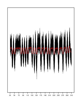
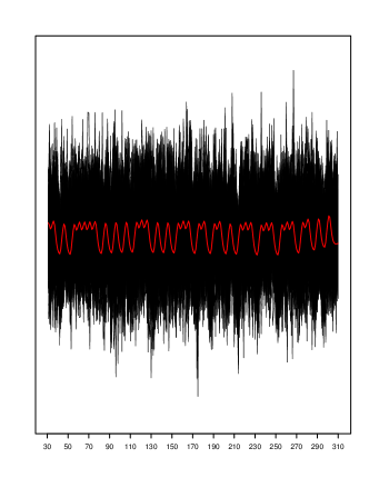
Figure 3: Simulated Bold response (black lines) and expected Bold response (red line) for an active (left) and non-active (right) voxel respectively.

posi.ffd = c(14, 56, 40)	posi.ffd = c(28, 67, 15)

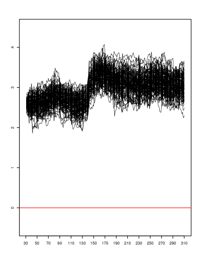
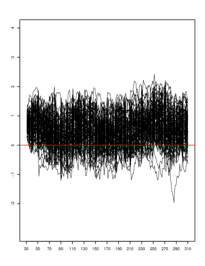
Figure 4: Simulated online trajectories of the state parameter for an active (left) and nonactive (right) volxel respectively.

Group analysis

Now we ilustrate how to run an fMRI group analysis as it is described in (RefARchive2). First, we read the fMRI images of 21 subjects from the "voice-localizer" example:

R> names <- list.files("~/fMRIData/")R> names

using the "Joint" as sampler distribution.

 [1] "sub-001.nii.gz" "sub-002.nii.gz" "sub-003.nii.gz" [4] "sub-004.nii.gz" "sub-005.nii.gz" "sub-006.nii.gz" [7] "sub-007.nii.gz" "sub-008.nii.gz" "sub-009.nii.gz"[10] "sub-010.nii.gz" "sub-011.nii.gz" "sub-012.nii.gz"[13] "sub-013.nii.gz" "sub-014.nii.gz" "sub-015.nii.gz"[16] "sub-016.nii.gz" "sub-017.nii.gz" "sub-018.nii.gz"[19] "sub-019.nii.gz" "sub-020.nii.gz" "sub-021.nii.gz"

R> DataGroups <- function(x){+   ffd.c2 <- readNIfTI(paste("~/fMRIParietal/",x, sep=""), reorient = FALSE)+   ffd.c <- ffd.c2@.Data+   return(ffd.c)+ }R> system.time(DatabaseGroup <- parLapply(names, DataGroups, cl = 7))   user  system elapsed637.016 923.008 400.528R> str(DatabaseGroup)

List of 21 $ : num [1:91, 1:109, 1:91, 1:310] 0 0 0 0 0 0 0 0 0 0 ... $ : num [1:91, 1:109, 1:91, 1:310] 0 0 0 0 0 0 0 0 0 0 ... $ : num [1:91, 1:109, 1:91, 1:310] 0 0 0 0 0 0 0 0 0 0 ... $ : num [1:91, 1:109, 1:91, 1:310] 0 0 0 0 0 0 0 0 0 0 ... $ : num [1:91, 1:109, 1:91, 1:310] 0 0 0 0 0 0 0 0 0 0 ... $ : num [1:91, 1:109, 1:91, 1:310] 0 0 0 0 0 0 0 0 0 0 ... $ : num [1:91, 1:109, 1:91, 1:310] 0 0 0 0 0 0 0 0 0 0 ... $ : num [1:91, 1:109, 1:91, 1:310] 0 0 0 0 0 0 0 0 0 0 ...

In order to run any of the functions available in this package to perform fMRI group analysis, the datasets or set of images from each subject must be stored on a list object as it is shown above. To deal with this huge amount of information the user has to have a big RAM memory capacity available on the machine where this process is going to be run. It is also recommended to have a multi-core processor available in order to speed up computation time. The arguments or input parameters for any of the functions offered in this package to run group analysis are almost the same as those required for individual analysis. There is only an additional argument needed (mask), which adds a 3D array that works as a brain of reference (MNI atlas) for the group analysis.

R> MASK <- readNIfTI("~/mask.nii.gz")

R> res <- ffdGroupEvidenceFEST(ffdGroup = DatabaseGroup,+ covariates = Covariates, m0 = 0, Cova = 100, delta = 0.95, S0 = 1,+ n0 = 1, N1 = FALSE, Nsimu1 = 100, Cutpos=30, r1 = 1, Test = "Joint",+ mask = MASK, Ncores = 7)

 |++++++++++++++++++++++++++++++++++++++++++++++++++| 100% elapsed = 53m 45s

R> str(res)

List of 4 $ : num [1:91, 1:109, 1:91] 0 0 0 0 0 0 0 0 0 0 ... $ : num [1:91, 1:109, 1:91] 0 0 0 0 0 0 0 0 0 0 ... $ : num [1:91, 1:109, 1:91] 0 0 0 0 0 0 0 0 0 0 ... $ : num [1:91, 1:109, 1:91] 0 0 0 0 0 0 0 0 0 0 ...

ffdGroupEvidenceFEST returns an array of dimension $2\times p$ elements, where $p$ is the number of covariates and $2$ is the number of options evaluated as sampler distributions: "Joint" and "Marginal". The first $p$ elements are the 3D arrays related to each column of the covariates matrix respectively when computing the activation evidence using the "Join" distribution. The ramaining arrays are those related to the marginal distribution.

R> res2 <- ffdGroupEvidenceFFBS(ffdGroup = DatabaseGroup, covariates = Covariates,+ m0=0, Cova=100, delta = 0.95, S0 = 1, n0 = 1, N1 = FALSE, Nsimu1 = 100,+ Cutpos = 30, r1 = 1, mask = MASK, Ncores = 7)

 |++++++++++++++++++++++++++++++++++++++++++++++++++| 100% elapsed = 44m 49s

R> str(res2)

List of 3 $ : num [1:2, 1:91, 1:109, 1:91] 0 0 0 0 0 0 0 0 0 0 ... $ : num [1:2, 1:91, 1:109, 1:91] 0 0 0 0 0 0 0 0 0 0 ... $ : num [1:2, 1:91, 1:109, 1:91] 0 0 0 0 0 0 0 0 0 0$ ...

ffdGroupEvidenceFFBS returns an 3D array with the same structure and characteristics as its individual counterpart.

R> library(neurobase)R> res.auxi <- res2[[1]][1,,,]R> ffd <- readNIfTI("standard.nii.gz")R> Z.visual.c <- nifti(res.auxi, datatype=16)R> ortho2(ffd, ifelse(Z.visual.c > 0.95, Z.visual.c, NA),+  col.y = heat.colors(50), ycolorbar = TRUE, ybreaks = seq(0.95, 1, by = 0.001))

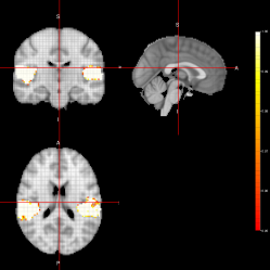
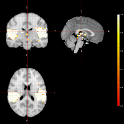
Figure 5: Activations maps obtained with the functions ffdGroupEvidenceFEST (left) and ffdGroupEvidenceFFBS (right) using the "Joint" as sampler distribution.

The functioning of the functions for single-voxel analysis at the group stage is the same as their counterparts at the individual stage.

R> resSingle <- GroupSingleVoxelFEST(posi.ffd = c(14, 56, 40), DatabaseGroup,+ covariates = Covariates, m0 = 0, Cova = 100, delta = 0.95, S0 = 1, n0 = 1,+ N1 = FALSE, Nsimu1 = 100, r1 = 1, Test = "Joint", Cutpos = 30)

R> frame()R> plot.window(xlim=c(30, 311), ylim = c(-5, 5))axis(1, at=seq(30, 310, by = 20), lwd = 2, xlab = "Time")R> box(lwd = 2)R> for(j in 2:7){for(i in 1:dim(resSingle[[4]])[1]){lines(31:dim(covariates)[1],+ resSingle[[4]][i, j,], col = "green")}}R> for(i in 1:dim(resSingle[[4]])[1]){lines(31:dim(covariates)[1],+ resSingle[[4]][i, 1,], col = "black")}lines(31:dim(covariates)[1], covariates[31:dim(covariates)[1], 1],+ col = "red", lwd = 2)

posi.ffd = c(14, 56, 40)	posi.ffd = c(28, 67, 15)

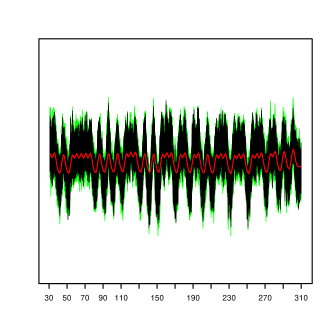
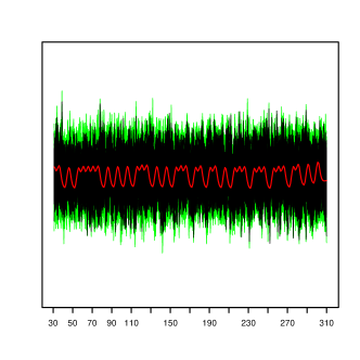
Figure 6: The black curves are simulated BOLD responses for voxel at position posi.ffd and the green curves are the BOLD responses related to its neighbors. The red curve is the expected BOLD response for the "voice localizer" experiment.

posi.ffd = c(14, 56, 40)	posi.ffd = c(28, 67, 15)

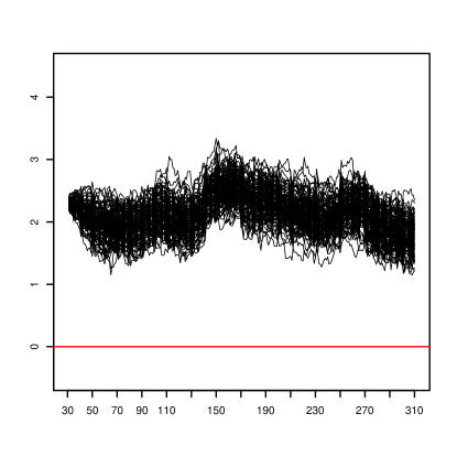
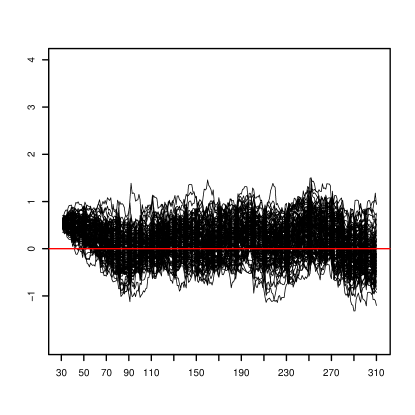
Figure 7: Simulated online trajectories of the state parameter for an active (left) and nonactive (right) volxel respectively.

R> frame()R> plot.window(xlim=c(30, 311), ylim=c(-0.5, 4.5), ylab = expression(theta))R> axis(1, at=seq(30, 310, by = 20), lwd = 2, xlab = "Time")R> axis(2, at=-1:4, lwd=2)R> box(lwd = 2)R> for(i in 1:dim(resSingle[[3]])[3]){lines(31:dim(covariates)[1],resSingle[[3]][1, , i])}R> abline(h = 0, col = "red" , lwd = 2)

4 Conclusions and future work

In this work, we present the BayesDLMfMRI package, which allows performing statistical analysis for fMRI data at individual and group stages. It offers different options to assess brain activation for single voxels as well as the entire brain volume and/or more specific brain regions with the help of a mask. The low-level functions are written in C++ and options for parallel computation are available in some of the functions. Currently, some extensions for this package related to comparisons between groups and comparisons between tasks as well as other relevant features are being developed.

Computational details

The results in this paper were obtained using R 3.4.4 with the Rcpp 1.0.2, RcppArmadillo 0.9.200.5.0 and pbapply 1.4.2 packages on a computer with Linux-Ubuntu, 32 CPUs and 188GB of RAM. R itself and all packages used are available from the Comprehensive R Archive Network (CRAN) at https://CRAN.R-project.org/.

References

- Zhang et al. [2016] Linlin Zhang, Michele Guindani, Francesco Versace, Jeffrey M Engelmann, Marina Vannucci, et al. A spatiotemporal nonparametric bayesian model of multi-subject fmri data. The Annals of Applied Statistics, 10(2):638–666, 2016.
- Eklund et al. [2017] Anders Eklund, Martin A Lindquist, and Mattias Villani. A bayesian heteroscedastic glm with application to fmri data with motion spikes. NeuroImage, 155:354–369, 2017.
- Bezener et al. [2018] Martin Bezener, John Hughes, Galin Jones, et al. Bayesian spatiotemporal modeling using hierarchical spatial priors, with applications to functional magnetic resonance imaging. Bayesian Analysis, 2018.
- Yu et al. [2018] Cheng-Han Yu, Raquel Prado, Hernando Ombao, and Daniel Rowe. A bayesian variable selection approach yields improved detection of brain activation from complex-valued fmri. Journal of the American Statistical Association, (just-accepted):1–61, 2018.
- Zhang et al. [2015] Linlin Zhang, Michele Guindani, and Marina Vannucci. Bayesian models for fmri data analysis. Wiley interdisciplinary reviews. Computational statistics, 7(1):21–41, 2015.
- Jenkinson et al. [2012] Mark Jenkinson, Christian F Beckmann, Timothy EJ Behrens, Mark W Woolrich, and Stephen M Smith. Fsl. Neuroimage, 62(2):782–790, 2012.
- Penny et al. [2011] William D Penny, Karl J Friston, John T Ashburner, Stefan J Kiebel, and Thomas E Nichols. Statistical parametric mapping: the analysis of functional brain images. Elsevier, 2011.
- Kook et al. [2019] Jeong Hwan Kook, Michele Guindani, Linlin Zhang, and Marina Vannucci. Npbayes-fmri: Non-parametric bayesian general linear models for single-and multi-subject fmri data. Statistics in Biosciences, 11(1):3–21, 2019.
- R Core Team [2018] R Core Team. R: A Language and Environment for Statistical Computing. R Foundation for Statistical Computing, Vienna, Austria, 2018. URL https://www.R-project.org/.
- Tabelow and Polzehl [2011] Karsten Tabelow and Jörg Polzehl. Statistical parametric maps for functional mri experiments in R: The package fmri. Journal of Statistical Software, 44(11):1–21, 2011. URL http://www.jstatsoft.org/v44/i11/.
- Whitcher et al. [2011] Brandon Whitcher, Volker J. Schmid, and Andrew Thornton. Working with the DICOM and NIfTI data standards in R. Journal of Statistical Software, 44(6):1–28, 2011. URL http://www.jstatsoft.org/v44/i06/.
- Muschelli [2018] John Muschelli. neurobase: ’Neuroconductor’ Base Package with Helper Functions for ’nifti’ Objects, 2018. URL https://CRAN.R-project.org/package=neurobase. R package version 1.27.6.
- Welvaert et al. [2011] Marijke Welvaert, Joke Durnez, Beatrijs Moerkerke, Geert Verdoolaege, and Yves Rosseel. neurosim: An r package for generating fmri data. Journal of Statistical Software, 44(10):1–18, 2011.
- da Silva et al. [2011] AR Ferreira da Silva et al. cudabayesreg: parallel implementation of a bayesian multilevel model for fmri data analysis. Journal of Statistical Software, 44(4):1–24, 2011.
- Sanyal and Ferreira [2019] Nilotpal Sanyal and Marco A.R. Ferreira. BHMSMAfMRI: Bayesian Hierarchical Multi-Subject Multiscale Analysis of Functional MRI Data, 2019. URL https://CRAN.R-project.org/package=BHMSMAfMRI. R package version 1.3.
- Jiménez et al. [2019] Johnatan Cardona Jiménez, Carlos A. de B. Pereira, and Victor Fossaluza. Assessing dynamic effects on a bayesian matrix-variate dynamic linear model: an application to fmri data analysis. arXiv:1910.12058, 2019.
- Jiménez [2019] Johnatan Cardona Jiménez. fmri group analysis based on outputs from matrix-variate dynamic linear models. arXiv:1911.00708, 2019.
- Quintana [1985] Jose Mario Quintana. A dynamic linear matrix–variate regression model, 1985.
- Eddelbuettel et al. [2011] Dirk Eddelbuettel, Romain François, J Allaire, Kevin Ushey, Qiang Kou, N Russel, John Chambers, and D Bates. Rcpp: Seamless r and c++ integration. Journal of Statistical Software, 40(8):1–18, 2011.
- Eddelbuettel and Sanderson [2014] Dirk Eddelbuettel and Conrad Sanderson. Rcpparmadillo: Accelerating r with high-performance c++ linear algebra. Computational Statistics and Data Analysis, 71:1054–1063, March 2014. URL http://dx.doi.org/10.1016/j.csda.2013.02.005.
- Solymos and Zawadzki [2019] Peter Solymos and Zygmunt Zawadzki. pbapply: Adding Progress Bar to ’*apply’ Functions, 2019. URL https://CRAN.R-project.org/package=pbapply. R package version 1.4-1.
- Quintana [1987] Jose Mario Quintana. Multivariate Bayesian forecasting models. PhD thesis, University of Warwick, 1987.
- Pernet et al. [2015] Cyril R Pernet, Phil McAleer, Marianne Latinus, Krzysztof J Gorgolewski, Ian Charest, Patricia EG Bestelmeyer, Rebecca H Watson, David Fleming, Frances Crabbe, Mitchell Valdes-Sosa, et al. The human voice areas: Spatial organization and inter-individual variability in temporal and extra-temporal cortices. Neuroimage, 119:164–174, 2015.
- Gorgolewski et al. [2017] Krzysztof Gorgolewski, Oscar Esteban, Gunnar Schaefer, Brian Wandell, and Russell Poldrack. Openneuro - a free online platform for sharing and analysis of neuroimaging data. Organization for Human Brain Mapping. Vancouver, Canada, 1677, 2017.
- Quintana and West [1987] Jose Mario Quintana and Mike West. An analysis of international exchange rates using multivariate dlm’s. The Statistician, pages 275–281, 1987.
- Brett et al. [2002] Matthew Brett, Ingrid S Johnsrude, and Adrian M Owen. The problem of functional localization in the human brain. Nature reviews neuroscience, 3(3):243, 2002.