FC-based shock-dynamics solver with neural-network localized artificial-viscosity assignment

Abstract

This paper presents a spectral scheme for the numerical solution of nonlinear conservation laws in non-periodic domains under arbitrary boundary conditions. The approach relies on the use of the Fourier Continuation (FC) method for spectral representation of non-periodic functions in conjunction with smooth localized artificial viscosity assignments produced by means of a Shock-Detecting Neural Network (SDNN). Like previous shock capturing schemes and artificial viscosity techniques, the combined FC-SDNN strategy effectively controls spurious oscillations in the proximity of discontinuities. Thanks to its use of a localized but smooth artificial viscosity term, whose support is restricted to a vicinity of flow-discontinuity points, the algorithm enjoys spectral accuracy and low dissipation away from flow discontinuities, and, in such regions, it produces smooth numerical solutions—as evidenced by an essential absence of spurious oscillations in level set lines. The FC-SDNN viscosity assignment, which does not require use of problem-dependent algorithmic parameters, induces a significantly lower overall dissipation than other methods, including the Fourier-spectral versions of the previous entropy viscosity method. The character of the proposed algorithm is illustrated with a variety of numerical results for the linear advection, Burgers and Euler equations in one and two-dimensional non-periodic spatial domains.

Keywords: Machine learning, Neural networks, Shocks, Artificial viscosity, Conservation laws, Fourier continuation, Non-periodic domain, Spectral method

1 Introduction

This paper presents a new “FC-SDNN” spectral scheme for the numerical solution of nonlinear conservation laws under arbitrary boundary conditions. The proposed approaches relies on use of the FC-Gram Fourier Continuation method [1, 2, 5, 28] for spectral representation of non-periodic functions in conjunction with localized smooth artificial viscosity assignments prescribed by means of the neural network-based shock-detection method proposed in [37]. The neural network approach [37] itself utilizes Fourier series to discretize the gas dynamics and related equations, and it eliminates Gibbs ringing at shock positions (which are determined by means of an artificial neural network) by assigning artificial viscosity over a small number of discrete points in a close vicinity of shocks. The use of the classical Fourier spectral method in that contribution restricts the method’s applicability to periodic problems (so that, in particular, the outer computational boundaries cannot be physical boundaries), and its highly localized viscosity assignments give rise to a degree of non-smoothness, resulting in certain types of unphysical oscillations manifested as serrated level-set lines in the flow fields. The FC-SDNN method presented in this paper addresses these challenges. In particular, in view of its use of certain newly-designed smooth viscosity windows introduced in Section 3.3, the method avoids the introduction of roughness in the viscosity assignments and thus it yields smooth flows away from shocks and other flow discontinuities. In addition, the underlying FC-Gram spectral representations enable applicability to general non-periodic problems, and, in view of the weak local viscosity assignments used, it gives rise to sharp resolution of shocks. As a result, and as demonstrated in this paper via application to a range of well known 1D and 2D shock-wave test configurations, the overall FC-SDNN approach yields accurate and essentially oscillation-free solutions for general non-periodic problems.

The computational solution of systems of conservation laws has been tackled by means of a variety of numerical methods, including low-order finite volume [25, 26] and finite difference methods equipped with slope limiters [25, 26], as well as higher order shock-capturing methods such as the ENO [14] and WENO schemes [27, 16]. An efficient FC/WENO hybrid solver was proposed in [38]. The use of artificial viscosity as a computational device for conservation laws, on the other hand, was first proposed in [36, 44] and the subsequent contributions[21, 22, 9]. The viscous terms proposed in these papers, which incorporate derivatives of the square of the velocity gradient, may induce oscillations in the vicinity of shocks [22] (since the velocity itself is not smooth in such regions), and, as they do not completely vanish away from the discontinuities, they may lead to significant approximation errors in regions were the fluid velocity varies rapidly. Reference [31] proposes the use of a shock-detecting sensor in order to localize the support of the artificial viscosity, which is used in the context of a Discontinuous Galerkin scheme.

The entropy viscosity method [13] (EV) incorporates a nonlinear viscous “entropy-residual” term which essentially vanishes away from discontinuities—in view of the fact that the flow is isentropic over smooth flow regions—and which is thus used to limit non-zero viscosity assignments to regions near flow discontinuities, including both shock waves and contact discontinuities. This method, however, relies on several problem-dependent algorithmic parameters that require tuning for every application. Additionally, this approach gives rise to a significant amount of dissipation even away from shocks, in particular in the vicinity of contact discontinuities and regions containing fast spatial variation in the flow-field variables. Considerable improvements concerning this issue were obtained in [20] (which additionally introduced a Hermite-based method to discretize the hyperbolic systems) by modifying the EV viscosity term. Like the viscous term introduced by [44], the EV viscosity assignments [13, 20] are themselves discontinuous in the vicinity of shocks, and, thus, their use may introduce spurious oscillations. The C-method [35, 32, 33], which augments the hyperbolic system with an additional equation used to determine a spatio-temporally smooth viscous term, relies, like the EV method, on use of several problem dependent parameters and algorithmic variations.

Recently, significant progress was made by incorporating machine learning-based techniques (ML) to enhance the performance of classical shock capturing schemes [34, 8, 42, 37]. The approach [34, 8, 37] utilizes ML-based methods to detect discontinuities which are then smeared by means of shock-localized artificial viscosity assignments in the context of various discretization methods, including Discontinuous Galerkin schemes [34, 8] and Fourier spectral schemes [37]. The ML-based approach utilized in [42], in turn, modifies the finite volume coefficients utilized in the WENO5-JS scheme by learning small perturbations of these coefficients leading to improved accurate representations of functions at cell boundaries.

Like the strategy underlying the contribution [37], the FC-SDNN method proposed in this paper relies on the occurrence of Gibbs oscillations for ML-based shock detection. Unlike the previous approach, however, the present method assigns a smooth (albeit also shock-localized) viscous term. In view of its smooth viscosity assignments this procedure effectively eliminates Gibbs oscillations while avoiding introduction of the flow-field roughness that is often evidenced by the serrated level sets produced by other methods. In view of its use of FC-based Fourier expansions, further, the proposed algorithm enjoys spectral accuracy away from shocks (thus, delivering, in particular, essentially vanishing dispersion in such regions; see Section 2.3 and Figure 6) while enabling solution under general (non-periodic) boundary conditions. Unlike other techniques, finally, the approach does not require use of problem-dependent algorithmic parameters.

The capabilities of the proposed algorithm are illustrated by means of a variety of numerical results, in one and two-dimensional contexts, for the Linear Advection, Burgers and Euler equations. In order to provide a useful reference point, this paper also presents an FC-based version, termed FC-EV, of the EV algorithm [13]. (The modified version [20] of the entropy viscosity approach, which was also tested as a possible reference solver, was not found to be completely reliable in our FC-based context, since it occasionally led to spurious oscillations in shock regions as grids were refined, and the corresponding results were therefore not included in this paper.) We find that the FC-SDNN algorithm generally provides significantly more accurate numerical approximations than the FC-EV, as the localized artificial viscosity in the former approach induces a much lower dissipation level than the latter.

This paper is organized as follows. After necessary preliminaries are presented in Section 2 (concerning the hyperbolic problems under consideration, as well as the Fourier Continuation method, and including basic background on the artificial-viscosity strategies we consider), Section 3 describes the proposed FC-SDNN approach. Section 4 then demonstrates the algorithm’s performance for a variety of non-periodic linear and nonlinear hyperbolic problems. In particular, cases are considered for the linear advection equation, Burgers equation and Euler’s equations in one-dimensional and two-dimensional rectangular and non-rectangular spatial domains, including cases in which shock waves meet smooth and non-smooth physical boundaries.

2 Preliminaries

2.1 Conservation laws

This paper proposes novel spectral methodologies, applicable in general non-periodic contexts and with general boundary conditions, for the numerical solution of conservation-law equations of the form

$$\dfrac{\partial}{\partial t}\textit{{e}}(\textit{{x}},t)+\nabla\cdot\big{(}f(\textit{{e}}(\textit{{x}},t))\big{)}=0$$ (1)

on a bounded domain $\Omega\subset\mathbb{R}^{q}$, where $\textit{{e}}:\Omega\times[0,T]\rightarrow\mathbb{R}^{r}$ and $f:\mathbb{R}^{r}\rightarrow\mathbb{R}^{r}\times\mathbb{R}^{q}$ denote the unknown solution vector and a (smooth) convective flux, respectively.

The proposed spectral approaches are demonstrated for several equations of the form (1), including the Linear Advection equation

$$\frac{\partial u}{\partial t}+a\frac{\partial u}{\partial x}=0$$ (2)

with a constant propagation velocity $a$, where we have $\textit{{e}}=u$, and $f(u)=au$; the one- and two-dimensional scalar Burgers equations

$$\frac{\partial u}{\partial t}+\frac{1}{2}\Big{(}\frac{\partial u^{2}}{\partial x}\Big{)}=0$$ (3)

and

$$\frac{\partial u}{\partial t}+\frac{1}{2}\Big{(}\frac{\partial u^{2}}{\partial x}\Big{)}+\frac{1}{2}\Big{(}\frac{\partial u^{2}}{\partial y}\Big{)}=0,$$ (4)

for each of which we have $\textit{{e}}=u$ and $f(u)=\frac{u^{2}}{2}$; as well as the one- and two-dimensional Euler equations

$$\dfrac{\partial}{\partial t}\begin{pmatrix}\ \rho\\[3.0pt] \ \rho u\\[3.0pt] \ E\end{pmatrix}+\frac{\partial}{\partial x}\begin{pmatrix}\ \rho u\\[3.0pt] \ \rho u^{2}+p\\[3.0pt] \ u(E+p)\end{pmatrix}=0$$ (5)

and

$$\dfrac{\partial}{\partial t}\begin{pmatrix}\ \rho\\[3.0pt] \ \rho u\\[3.0pt] \ \rho v\\[3.0pt] \ E\end{pmatrix}+\frac{\partial}{\partial x}\begin{pmatrix}\ \rho u\\[3.0pt] \ \rho u^{2}+p\\[3.0pt] \ \rho uv\\[3.0pt] \ u(E+p)\end{pmatrix}+\frac{\partial}{\partial y}\begin{pmatrix}\ \rho v\\[3.0pt] \ \rho uv\\[3.0pt] \ \rho v^{2}+p\\[3.0pt] \ v(E+p)\end{pmatrix}=0$$ (6)

with

$$E=\frac{p}{\gamma-1}+\frac{1}{2}\rho\lvert\textit{{u}}\rvert^{2},$$ (7)

for each of which we have

$$\textit{{e}}=(\rho,\rho\textit{{u}},E)^{T},\quad f(\textit{{e}})=(\rho\textit{{u}},\rho\textit{{u}}\otimes\textit{{u}}+p\mathbb{I},\textit{{u}}(E+p))^{T}.$$ (8)

Here $\mathbb{I}$ denotes the identity tensor, $\textbf{a}\otimes\textbf{b}=(a_{i}b_{j})$ denotes the tensor product of the vectors $\textbf{a}=(a_{i})$ and $\textbf{b}=(b_{j})$, and $\rho$, u, $E$ and $p$ denote the density, velocity vector, total energy and pressure, respectively. The speed of sound [25]

$$a=\sqrt{\frac{\gamma p}{\rho}}$$ (9)

for the Euler equations plays important roles in the various artificial viscosity assignments considered in this paper for Euler problems in both 1D and 2D.

Remark 1.

As an example concerning notational conventions, note that in the case of the 2D Euler equations, for which $f$ is given by (8), $\nabla\cdot\big{(}f(\textit{{e}})\big{)}$ can be viewed as a three coordinate vector whose first, second and third coordinates are a scalar, a vector and a scalar, respectively. Using the Einstein summation convention, these three components are respectively given by $\nabla\cdot(\rho\textbf{u})=\partial_{i}(\rho u_{i})$, $\big{(}\nabla\cdot(\rho\textit{{u}}\otimes\textit{{u}}+p\mathbb{I})\big{)}_{j}=\partial_{i}(\rho u_{j}u_{i}+p)$ and $\nabla\cdot((E+p)\textbf{u})=\partial_{i}((E+p)u_{i})$.

2.2 Artificial viscosity

As is well known, the shocks and other flow discontinuities that arise in the context of nonlinear conservation laws of the form (1) give rise to a number of challenges from the point of view of computational simulation. In particular, in the framework of classical finite difference methods as well as Fourier spectral methods, such discontinuities are associated with the appearance of spurious “Gibbs oscillations”. Artificial viscosity methods aim at tackling this difficulty by considering, instead of the inviscid equations (1), certain closely related equations which include viscous terms containing second order spatial derivatives. Provided the viscous terms are adequately chosen and sufficiently small, the resulting solutions, which are smooth functions on account of viscosity, approximate well the desired (discontinuous) inviscid solutions. In general terms, the viscous equations are obtained by adding a viscous term of the form $\nabla\cdot\big{(}f_{\textit{visc}}[\textit{{e}}]\big{)}$ to the right hand side of (1), where the “viscous flux” operator

$$f_{\textit{visc}}[\textit{{e}}]=\mu[\textit{{e}}]\mathbf{D}[\textit{{e}}],$$ (10)

(which, for a given vector-valued function $\textbf{e}(x,t)$, produces a vector-valued function $f_{\textit{visc}}[\textit{{e}}](x,t)$ defined in the complete computational domain), is given in terms of a certain “viscosity” operator $\mu[\textit{{e}}](x,t)$ (which may or may not include derivatives of the flow variables e), and a certain matrix-valued first order differential operator $\mathbf{D}$. Once such a viscous term is included, the viscous equation

$$\frac{\partial\textit{{e}}(\textit{{x}},t)}{\partial t}+\nabla\cdot\big{(}f(\textit{{e}}(\textit{{x}},t))\big{)}=\nabla\cdot\big{(}f_{\textit{visc}}[\textit{{e}}](\textit{{x}},t)\big{)}$$ (11)

results.

Per the discussion in Section 1, this paper exploits and extends, in the context of the Fourier-Continuation discretizations, two different approaches to viscosity-regularization—each one resulting from a corresponding selection of the operators $\mu$ and $\mathbf{D}$. One of these approaches, the EV method, produces a viscosity assignment $\mu[\textit{{e}}](x,t)$ on the basis of certain differential and algebraic operations together with a number of tunable problem-dependent parameters that are specifically designed for each particular equation considered, as described in Section 2.2.2. The resulting viscosity values $\mu[\textit{{e}}](x,t)$ are highest in a vicinity of discontinuity regions and decrease rapidly away from such regions. The neural-network approach introduced in Section 2.2.1, in turn, uses machine learning methods to pinpoint the location of discontinuities, and then produces a viscosity function whose support is restricted to a vicinity of such discontinuity locations. As a significant advantage, the neural-network method, which does not require use of tunable parameters, is essentially problem independent, and it can use a single pre-trained neural network for all the equations considered. Details concerning these two viscosity-assignment methods considered are provided in what follows.

2.2.1 Artificial viscosity via shock-detecting neural network (SDNN)

The SDNN approach proposed in this paper is based on the neural-network strategy introduced in [37] for detection of discontinuities on the basis of Gibbs oscillations in Fourier series, together with a novel selection of the operator $\mu$ in (10) that yields spatially localized but smooth viscosity assignments: per the description in Section 3.3, the FC-SDNN viscosity $\mu[\textit{{e}}](\textit{{x}},t)$ is a smooth function that vanishes except in narrow regions around flow discontinuities. The differential operator $\mathbf{D}$, in turn, is simply given by

$$\mathbf{D}[\textit{{e}}](\textit{{x}},t)=\nabla(\textit{{e}}(\textit{{x}},t)),$$ (12)

where the gradient is computed component-wise. As indicated in Section 1, the smoothness of the proposed viscosity assignments is inherited by the resulting flows away from flow discontinuities, thus helping eliminate the serrated level-set lines that are ubiquitous in the flow patterns produced by other methods.

2.2.2 Entropy viscosity methodology (EV)

The operators $\mu$ and $\mathbf{D}$ employed by the EV approach [13] are defined in terms of a number of problem dependent functions, vectors and operators. Indeed, starting with an equation dependent entropy pair $(\eta,\nu)$ where $\eta$ is a scalar function and $\nu$ is a vector of the same dimensionality as the velocity vector, the EV approach utilizes an associated scalar entropy residual operator

$$R_{EV}[\textit{{e}}](\textit{{x}},t)=\frac{\partial\eta(\textit{{e}}(\textit{{x}},t))}{\partial t}+\nabla\cdot\nu(\textit{{e}}(\textit{{x}},t))$$ (13)

together with a function $C=C(\textit{{e}})$ related to the local wave speed, and a normalization operator $N=N[e](x,t)$ obtained from the function $\eta$.

In practice, reference [13] proposes $\eta(\textit{{e}})=\frac{u^{2}}{2}$, $\nu(\textit{{e}})=a\frac{u^{2}}{2}$ and $C(\textit{{e}})=a$ for the Linear Advection equation (2), $\eta(\textit{{e}})=\frac{u^{2}}{2}$, $\nu(\textit{{e}})=\frac{u^{3}}{3}$ and $C(\textit{{e}})=u$ for the 1D and 2D Burgers equations (3) and (4), and $\eta(\textit{{e}})=\frac{\rho}{\gamma-1}\log(p/\rho^{\gamma})$, $\nu(\textit{{e}})=\textit{{u}}\frac{\rho}{\gamma-1}\log(p/\rho^{\gamma})$ and $C(\textit{{e}})=\|\textit{{u}}\|+a$ (where $a$ denotes the speed of sound (9)) for the 1D and 2D Euler equations (5) and (6). As for the normalization operator, reference [13] proposes $N=1$ for the Euler equations and $N[e](x,t)=|\eta(e)(x,t)-\overline{\eta}(e)(t)|$ for the Linear advection and Burgers equations, where $\overline{\eta}(e)(t)$ denotes the spatial average of $\eta(e)$ at time $t$.

For a numerical discretization with maximum spatial mesh size $h$, the EV viscosity function is defined by

$$\mu[\textit{{e}}](\textit{{x}},t)=\min(\mu_{\textit{max}}[\textit{{e}}](t),\mu_{E}[\textit{{e}}](\textit{{x}},t))$$ (14)

where the maximum viscosity $\mu_{\textit{max}}$ is given by

$$\mu_{\textit{max}}[\textit{{e}}](t)=c_{\textit{max}}h\max_{x\in\Omega}|C(\textit{{e}}(\textit{{x}},t))|$$ (15)

and where

$$\mu_{E}[\textit{{e}}](\textit{{x}},t)=c_{E}h^{2}\frac{|R_{EV}[\textit{{e}}](\textit{{x}},t)|}{N[\textit{{e}}](\textit{{x}},t)}.$$ (16)

In particular, the EV viscosity function depends on two parameters, $c_{\textit{max}}$ and $c_{E}$, both of size $\mathcal{O}(1)$, that, following [13], are to be tuned to each particular problem.

Finally, the EV differential operator $\mathbf{D}$ for the Linear Advection and Burgers equations is defined by

$$\mathbf{D}[\textit{{e}}](\textit{{x}},t)=\nabla(\textit{{e}}(\textit{{x}},t)),$$ (17)

while for the Euler equations it is given by

$$\mathbf{D}[\textit{{e}}](\textit{{x}},t)=\begin{pmatrix}\ 0\\[3.0pt] \ \frac{1}{2}(\nabla\textit{{u}}+(\nabla\textit{{u}})^{T})\\[3.0pt] \ \frac{1}{2}(\nabla\textit{{u}}+(\nabla\textit{{u}})^{T})\textit{{u}}+\kappa\nabla(p/\rho)\end{pmatrix}$$ (18)

where, using the Einstein notation $\left\{(\nabla\textit{{u}}+(\nabla\textit{{u}})^{T})\textit{{u}}\right\}_{i}=(\partial_{i}u_{j}+\partial_{j}u_{i})u_{j}$, and where $\kappa=\frac{\mathcal{P}}{\gamma-1}\mu$, with the Prandtl number $\mathcal{P}$ taken to equal 1.

2.3 Fourier Continuation spatial approximation

The straightforward Fourier-based discretization of nonlinear conservation laws generally suffers from crippling Gibbs oscillations resulting from two different sources: the physical flow discontinuities, on one hand, and the overall generic non-periodicity of the flow variables, on the other. Unlike the Gibbs ringing in flow-discontinuity regions, the ringing induced by lack of periodicity is not susceptible to treatment via artificial viscosity assignments of the type discussed in 2.2. In order to tackle this difficulty we resort to use of the Fourier Continuation (FC) method for equispaced-grid spectral approximation of non-periodic functions.

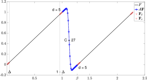
Figure 1: Fourier Continuation of the non-periodic function $F(x)=x$ on the interval $[0,1]$. With reference to the text, the red triangles (resp. squares), represent the $d=5$ left (resp. right) matching points, while the blue circles represent the $C=27$ continuation points.

The basic FC algorithm [1], called FC-Gram in view of its reliance on Gram polynomials for near-boundary approximation, constructs an accurate Fourier approximation of a given generally non-periodic function $F$ defined on a given one-dimensional interval—which, for definiteness, is assumed in this section to equal the unit interval $[0,1]$. The Fourier continuation algorithm relies on use of the function values $F_{j}=F(x_{j})$ of the function $F:[0,1]\to\mathbb{R}$ at $N$ points $x_{j}=jh\in[0,1]$ ($h=1/(N-1)$) to produce a function

$$F^{c}(x)=\sum^{M}_{k=-M}\hat{F}^{c}_{k}\exp(2\pi ikx/\beta)$$ (19)

which is defined (and periodic) in an interval $[0,\beta]$ that strictly contains $[0,1]$, where $\hat{F}^{c}_{k}$ denote the FC coefficients of $F$ and where, as detailed below, $M$ is an integer that, for $N$ large, is close to (but different from) the integer $\lfloor N/2\rfloor$.

In order to produce the FC function $F^{c}$, the FC-Gram algorithm first uses two subsets of the function values in the vector $\mathbf{F}=(F_{0},\dots,F_{N-1})^{T}$ (namely the function values at the“matching points” $\{x_{0},..,x_{d-1}\}$ and $\{x_{N-d},...,x_{N-1}\}$ located in small matching subintervals $[0,\Delta]$ and $[1-\Delta,1]$ of length $\Delta=(d-1)h$ near the left and right ends of the interval $[0,1]$, where $d$ is a small integer independent of $N$), to produce, at first, a discrete (but “smooth”) periodic extension vector $\mathbf{F}^{c}$ of the vector $\mathbf{F}$. Indeed, using the matching point data, the FC-Gram algorithm produces and appends a number $C$ of continuation function values in the interval $[1,\beta]$ to the data vector $\mathbf{F}$, so that the extension $\mathbf{F}^{c}$ transitions smoothly from $F_{N-1}$ back to $F_{0}$, as depicted in Figure 1. (The FC method can also be applied on the basis certain combinations of function values and derivatives by constructing the continuation vector $\mathbf{F}^{c}$, as described below in this section, on the basis of e.g. the vector $\mathbf{F}=(F_{0},\dots,F_{N-2},F^{\prime}_{N-1})^{T}$, where $F_{j}\approx F(x_{j})$ for $1\leq j\leq N-2$ and where $F^{\prime}_{N-1}\approx F^{\prime}(x_{N-1})$. Such a procedure enables imposition of Neumann boundary conditions in the context of the FC method.) The resulting vector $\mathbf{F}^{c}$ can be viewed as a discrete set of values of a smooth and periodic function which can be used to produce the Fourier continuation function $F^{c}$ via an application of the FFT algorithm. The function $F^{c}$ provides a spectral approximation of $F$ throughout the interval $[0,1]$ which does not suffer from either Gibbs-ringing or the associated interval-wide accuracy degradation. Throughout this paper we assume, for simplicity, that $N+C$ is an odd integer, and, thus, the resulting series has bandwidth $M=\frac{N+C-1}{2}$; consideration of even values of $N+C$ would require a slight modification of the index range in (19).

To obtain the necessary discrete periodic extension $\mathbf{F}^{c}$, the FC-Gram algorithm first produces two polynomial interpolants, one per matching subinterval, using, as indicated above, a small number $d$ of function values or a combination of function values and a derivative near each one of the endpoints of the interval $[0,1]$. This approach gives rise to high-order interpolation of the function $F$ over the matching intervals $[0,\Delta]$ and $[1-\Delta,1]$. The method for evaluation of the discrete periodic extension is based on a representation of these two polynomials in a particular orthogonal polynomials basis (the Gram polynomials), for each element of which the algorithm utilizes a precomputed smooth function which blends the basis polynomial to the zero function over the distance $\beta-1$ [1, 2]. Certain simple operations involving these “blending to zero” functions are then used, as indicated in these references and as illustrated in Figure 1, to obtain smooth transitions-to-zero from the left-most and right-most function values to the extension interval $[1,\beta]$. The values of this transition function at the points $N/(N-1),(N+1)/(N-1),\ldots,(N+C-1)/(N-1)$ provide the necessary $C$ additional point values from which, as mentioned above, the discrete extension $\mathbf{F}^{c}$ is obtained. The continuation function $F^{c}$ then easily results via an application of the FFT algorithm to the function values $F^{c}$ in the interval $[0,\beta]$.

The discrete continuation procedure can be expressed in the matricial form

$$\mathbf{F}^{c}=\begin{pmatrix}\mathbf{F}\\[3.0pt] A_{\ell}Q^{T}\mathbf{F}_{\ell}+A_{r}Q^{T}\mathbf{F}_{r}\end{pmatrix}$$ (20)

where the $d$-dimensional vectors $\mathbf{F}_{\ell}$ and $\mathbf{F}_{r}$ contain the point values of $F$ at the first and last $d$ discretization points in the interval $[0,1]$, respectively; where $Q$ is a $d\times d$ matrix, whose columns contain the point values of the elements of the Gram polynomial bases on the left matching intervals; and where $A_{\ell}$ and $A_{r}$ are $C\times d$, matrices containing the $C$ values of the blended-to-zero Gram polynomials in the left and right Gram bases, respectively. These small matrices can be computed once and stored on disc, and then read for use to produce FC expansions for functions $G:[a,b]\to\mathbb{R}$ defined on a given 1D interval $[a,b]$, via re-scaling to the interval $[0,1]$.

A minor modification of the procedure presented above suffices to produce a Fourier continuation function on the basis of data points at the domain interior and a derivative at interval endpoints. For example, given the vector $\mathbf{F}=(F_{0},\dots,F_{N-2},F^{\prime}_{N-1})^{T}$, using an adequately modified version $\widetilde{Q}$ of the matrix $Q$, an FC series $F^{c}(x)$ can be produced which matches the function values $F_{0},\dots,F_{N-2}$ at $x=x_{0},\dots,x_{N-2}$, and whose derivative equals $F^{\prime}_{N-1}$ at $x_{N-1}$. The matrix $\widetilde{Q}$ is obtained by using the matrix $Q$ to obtain a value $F_{N-1}$ such that the derivative $F^{\prime}(x_{N-1})$ equals the given value $F^{\prime}_{N-1}$. Full details in this regard can be found in [2, Sec. 3.2].

Clearly, the approximation order of the Fourier Continuation method (whether derivative values or function values are prescribed at endpoints) is restricted by the corresponding order $d$ of the Gram polynomial expansion, which, as detailed in various cases in Section 4, is selected as a small integer: $d=2$ or $d=5$. The relatively low order of accuracy afforded by the $d=2$ selection, which must be used in some cases to ensure stability, is not a matter of consequence in the context of the problems considered in the present paper, where high orders of accuracy are not expected from any numerical method on account of shocks and other flow discontinuities. Importantly, even in this context the FC method preserves one of the most significant numerical properties of Fourier series, namely its extremely small numerical dispersion. In fact, with exception of the cyclic advection example presented in Section 4.1.2, for which errors can accumulate on account of the spatio-temporal periodicity, for all cases in Section 4 for which both the $d=2$ and $d=5$ simulations were performed (which include those presented in Sections 4.1.1 (1D linear advection), 4.2.2 (2D Burgers equation) and 4.3.1 (1D Euler equations), the lower and higher order results obtained were visually indistinguishable.

The low dispersion character resulting from use of the FC method is demonstrated in Figure 6, which displays solutions produced by means of two different methods, namely, the FC-based order-5 FC-SDNN algorithm (Section 3) and the order-6 centered finite-difference scheme (both of which use the SSPRK-4 time discretization scheme), for a linear advection problem. The FC-SDNN solution presented in the figure does not deteriorate even for long propagation times, thus illustrating the essentially dispersion-free character of the FC-based approach. The finite-difference solution included in the Figure, in turn, does exhibit clear degradation with time, owing to the dispersion and diffusion effects associated with the underlying finite difference discretization.

3 FC-based time marching under neural network-controlled artificial viscosity

3.1 Spatial grid functions and spatio-temporal FC-based differentiation

We consider in this work 1D problems on intervals $I=[\xi_{\ell},\xi_{r}]$ as well as 2D problems on open domains $\Omega$ contained in rectangular regions $I\times J$, where $I=[\xi_{\ell},\xi_{r}]$ and $J=[\xi_{d},\xi_{u}]$ ($\xi_{\ell}<\xi_{r}$, $\xi_{d}<\xi_{u}$). Using a spatial meshsize $h$, the spatially discrete vectors of unknowns and certain related flow quantities will be represented by means of scalar and vector grid functions defined on 1D or 2D discretization grids of the form

$$G=\{x_{i}\ :\ x_{i}=x_{0}+ih,\quad i=0,\dots,N-1\}\quad(x_{0}=\xi_{\ell},\quad x_{N-1}=\xi_{r}),$$

and

$$G=\overline{\Omega}\cap\big{\{}(x_{i},y_{j})\ :\ x_{i}=x_{0}+ih,y_{j}=y_{0}+jh,0\leq i\leq N_{1}-1,\ 0\leq j\leq N_{2}-1\big{\}},$$

respectively. Here $\overline{\Omega}$ denotes the closure of $\Omega$, $x_{0}=\xi_{\ell}$, $x_{N_{1}-1}=\xi_{r}$, $y_{0}=\xi_{d}$ and $y_{N_{2}-1}=\xi_{u}$. In either case a function

$$b:G\to\mathbb{R}^{q}$$

will be called a “$q$-dimensional vector grid function”. Letting

$$\mathcal{I}=\big{\{}(i,j)\in\{0,\dots,N_{1}-1\}\times\{0,\dots,N_{2}-1\}\ :\ (x_{i},y_{j})\in G\big{\}},$$

we will also write $b(x_{i})=b_{i}$ ($0\leq i\leq N-1$) and $b(x_{i},y_{j})=b_{ij}$ ($(i,j)\in\mathcal{I}$). The set of $q$-dimensional vector grid functions defined on $G$ will be denoted by $\mathcal{G}^{q}$.

It is important to mention that, although the two-dimensional setting described above does not impose any restrictions on the character of the domain $\Omega$, for simplicity, the FC-SDNN solver presented in this paper assumes that the boundary of $\overline{\Omega}$ is given by a union of horizontal and vertical straight segments, each one of which runs along a Cartesian discretization line; see e.g. the Mach 3 forward-facing step case considered in Figure 16(a). Extensions to general domains $\Omega$, which could rely on either an embedded-boundary [5, 28, 6] approach, or an overlapping patch boundary-conforming curvilinear discretization strategy [1, 2, 4], is left for future work.

A spatially-discrete but time-continuous version of the solution vector $\textbf{{e}}(\mathbf{x},t)$ considered in Section 2 for 1D problems (resp. 2D problems) can be viewed as a time-dependent $q$-dimensional vector grid function $\textbf{{e}}_{i}=\textbf{{e}}_{i}(t)$ (resp. $\textbf{{e}}_{ij}=\textbf{{e}}_{ij}(t)$). Using $\textbf{{e}}_{h}=\textbf{{e}}_{h}(t)$ to refer generically to the $1D$ and $2D$ time-dependent grid functions $\textbf{{e}}_{i}$ and $\textbf{{e}}_{ij}$, the semidiscrete scheme for equation (11) becomes

$$\frac{d\textbf{{e}}_{h}(t)}{dt}=L[\textbf{{e}}_{h}(t)],$$ (21)

where $L$ denotes a consistent discrete approximation of the spatial operator in (11).

The discrete time evolution of the problem, on the other hand, is produced, throughout this paper, by means of the 4-th order strong stability preserving Runge-Kutta scheme (SSPRK-4) [12]—which, while not providing high convergence orders for the non-smooth solutions considered in this paper, does lead to low temporal dispersion and diffusion over smooth space-time regions of the computational domain. The corresponding time step is selected adaptively at each time-step $t=t_{n}$ according to the expression

$$\Delta t=\frac{\textrm{CFL}}{\pi(\frac{\max_{\textit{{x}}\in\Omega}\lvert S[\textit{{e}}](\mathbf{x},t)))\rvert}{h}+\frac{\max_{\textit{{x}}\in\Omega}\mu[\textit{{e}}](\textit{{x}},t)}{h^{2}})}.$$ (22)

Here CFL is a constant parameter that must be selected for each problem considered (as illustrated by the various selections utilized in Section 4), and $\mu[\textit{{e}}](\mathbf{x},t)$ and $S=S[\textit{{e}}](\mathbf{x},t)$ denote the artificial viscosity (equations (37) and (42)) and a maximum wave speed bound (MWSB) operator (which must be appropriately selected for each equation; see Section 3.3) at the spatio-temporal point $(\mathbf{x},t)$. (To avoid confusion we emphasize that equation (22) utilizes the maximum value for all $\mathbf{x}\in\Omega$ of the selected bound $S[\textit{{e}}](\mathbf{x},t)$ on the maximum wave speed.)

To obtain FC-based approximate derivatives of a function $F:K\to\mathbb{R}$ defined on a one-dimensional interval $K=[x_{0},x_{N-1}]$, whose values $(F_{0},F_{1},\dots,F_{N-1})^{T}$ are given on the uniform mesh $\{x_{0},x_{1},\dots,x_{N-1}\}$, the interval $K$ is re-scaled to $[0,1]$ and the corresponding continuation function $F^{c}$ is obtained by means of the FC-Gram procedure described in Section 2.3. The approximate derivatives at all mesh points are then obtained by applying the IFFT algorithm to the Fourier coefficients

$$(\hat{F}^{c})^{\prime}_{k}=\frac{2\pi ik}{\beta}\hat{F}^{c}_{k}.$$ (23)

of the derivative of the series (19) and re-scaling back to the interval $K$.

All of the numerical derivatives needed to evaluate the spatial operator $L[\textbf{{e}}_{h}(t)]$ are obtained via repeated application of the 1D FC differentiation procedure described above. For a function $F=F(x,y)$ defined on a two-dimensional domain $\Omega$ and whose values $F_{ij}$ ($(i,j)\in\mathcal{I}$) are given on a grid $G$ of the type described above in this section, for example, partial derivatives with respect to $x$ along the line $y=y_{j_{0}}$ for a relevant value of $j_{0}$ are obtained by differentiation of the FC expansion obtained for the function values $(F(x_{i},y_{j_{0}}))_{i}$ for integers $i$ such that $(i,j_{0})\in\mathcal{I}$. The $y$ differentiation process proceeds similarly. Mixed derivatives, finally, are produced by successive application of the $x$ and $y$ differentiation processes. Details concerning the filtered derivatives used in the proposed scheme are provided in Section 3.4.

The boundary conditions of Dirichlet and Neumann considered in this paper are imposed as part of the differentiation process described above. Dirichlet boundary conditions at time $t_{n,\nu}$ ($t_{n}<t_{n,\nu}\leq t_{n+1}$) corresponding to the $\nu$-th SSPRK-4 stage ($\nu=1,\dots,4$) for the time-step starting at $t=t_{n}$, are simply imposed by overwriting the boundary values of the unknown solution vector $\textit{{e}}_{h}$ obtained at time $t=t_{n,\nu}$ with the given boundary values at that time, prior to the evaluation of the spatial derivatives needed for the subsequent SSPRK-4 stage. Neumann boundary conditions are similarly enforced by constructing appropriate continuation vectors (Section 2.3) after each stage of the SSPRK-4 scheme on the basis of the modified pre-computed matrix $\widetilde{Q}$ mentioned in Section 2.3.

It is known that enforcement of the given physical boundary conditions at intermediate Runge-Kutta stages, which is referred to as the “conventional method” in [7], may lead to a reduced temporal order of accuracy at spatial points in a neighborhood of the boundary of the domain boundary. This is not a significant concern in the context of this paper, where the global order of accuracy is limited in view of the discontinuous character of the solutions considered. Alternative approaches that preserve the order of accuracy for smooth solutions, such as those introduced in [7, 30], could also be used in conjunction with the proposed approach. Another alternative, under which no boundary conditions are enforced at intermediate Runge-Kutta stages [19], can also be utilized in our context, but we have found the conventional method leads to smoother solutions near boundaries.

3.2 Neural network-induced smoothness-classification

3.2.1 Smoothness-classification operator and data pre-processing

The method described in the forthcoming Section 3.3 for determination of the artificial viscosity values $\mu[\textit{{e}}](\mathbf{x},t)$ (cf. also Section 2.2) relies on the “degree of smoothness” of a certain function $\Phi(\textit{{e}})(\mathbf{x},t)$ (called the “proxy variable”) of the unknown solution vector e. In detail, following [37], in this paper a proxy variable $\Phi(\textit{{e}})$ is used, which equals the velocity $u$, $\Phi(\textit{{e}})=u$, (resp. the Mach number, $\Phi(\textit{{e}})=\left\lVert\mathbf{u}\right\rVert\sqrt{\frac{\rho}{\gamma p}}$) for equations (2) through (4) (resp. equations (5) and (6)). The degree of smoothness of the function $\Phi(\textit{{e}})$ at a certain time $t$ is characterized by a smoothness-classification operator $\tau=\tau[\Phi(\textit{{e}})]$ that analyzes the oscillations in an FC expansion of $\Phi(\textit{{e}})$—which is itself obtained from the discrete numerical values $\bm{\phi}=\Phi(\textbf{{e}}_{h})$, so that, in particular, $\tau[\Phi(\textit{{e}})]=\tilde{\tau}[\bm{\phi}]$ for some discrete operator $\tilde{\tau}$. The determination (or, rather, estimation) of the degree of smoothness by the operator $\tilde{\tau}$ is effected on the basis of an Artificial Neural Network (ANN). (We introduce the operators $\tau$ and $\tilde{\tau}$ for the specific function $\Phi(\textbf{{e}})$, but, clearly, the algorithm applies to arbitrary scalar or vector functions, as can be seen e.g. in the application of these operators, in the context of network training, in Section 3.2.2.)

We first describe the operator $\tilde{\tau}=\tilde{\tau}[\bm{\phi}]$ for for a conservation law over a one-dimensional interval $I=[\xi_{\ell},\xi_{r}]$ discretized by an $N$-point equispaced mesh $(x_{0},\dots,x_{N-1})$ of mesh-size $h$, and for which FC expansions are obtained on the basis of the extended equispaced mesh $\{x_{0},\dots,x_{N+C-1}\}$. (Note that, in accordance with Section 2.3, this extended mesh includes the discrete points $\{x_{0},\dots,x_{N-1}\}$ in the interval $I$ as well as the discrete points $\{x_{N},\dots,x_{N+C-1}\}$ in the FC extension region.) In this case, the evaluation of the operator $\tilde{\tau}$ proceeds as follows.

1. Obtain the FC expansion coefficients $(\hat{\bm{\phi}}^{c}_{-M},\dots,\hat{\bm{\phi}}^{c}_{M})^{T}$ of $\Phi(\textbf{{e}})$ by applying the FC procedure described in Section 2.3 to the column vector $(\bm{\phi}_{0},\dots,\bm{\phi}_{N-1})^{T}$. (Note that in the present 1D case we have $\bm{\phi}_{j}=\Phi(\textbf{{e}}_{j})$.)

2. For a suitable selected non-negative number $\delta<h$, evaluate the values $\bm{\phi}^{(\delta)}_{j}$ ($0\leq j\leq N+C-1$ ) of the FC expansion obtained in point (i) at the shifted grid points $x_{0}+\delta,x_{1}+\delta,\dots,x_{N+C-1}+\delta$. This is achieved by applying the FFT algorithm to the “shifted” Fourier coefficients $\hat{\bm{\phi}}^{\delta}=(\hat{\bm{\phi}}^{\delta}_{-M},\dots,\hat{\bm{\phi}}^{\delta}_{M})$ where $\hat{\bm{\phi}}^{\delta}_{j}=\hat{\bm{\phi}}^{c}_{j}\exp(\frac{2\pi ij\delta}{\beta})$. Here, as in Section 2.3 and equation (19), $\beta$ denotes the length of the FC periodicity interval. Throughout this work, the value $\delta=\frac{h}{10}$ is used for classification of flow discontinuities. As indicated in Section 3.2.2, different values of $\delta$ are used in the training process.

3. For each $j\in\{0,\dots,N-1\}$, form the seven-point stencil

   $$\bm{\phi}^{(\delta,j)}=\big{(}\bm{\phi}^{(\delta)}_{m(j-3,N+C)},\dots,\bm{\phi}^{(\delta)}_{m(j,N+C)},\dots,\bm{\phi}^{(\delta)}_{m(j+3,N+C)}\big{)}^{T}$$

   of values of the shifted grid function obtained per point (ii). (Here, for an integer $0\leq j\leq P$, $m(j,P)$ denotes the remainder of $j$ modulo $P$, that is to say, $m(j,P)$ is the only integer between $0$ and $P-1$ such that $j-m(j,P)$ is an integer multiple of $P$. In view of the extended domain inherent in the continuation method, use of the remainder function $m$ allows for the smoothness classification algorithm to continue to operate correctly even at points $x_{j}$ near physical boundaries—for which the seven-point subgrid $(x_{j-3},\dots,x_{j},\dots,x_{j+3})$ may not be fully contained within the physical domain.)

4. Obtain the modified stencils $\widetilde{\bm{\phi}}^{(\delta,j)}=\big{(}\widetilde{\bm{\phi}}^{(\delta)}_{m(j-3,N+C)},\ldots,\widetilde{\bm{\phi}}^{(\delta)}_{m(j,N+C)},\ldots\widetilde{\bm{\phi}}^{(\delta)}_{m(j+3,N+C)}\big{)}^{T}$ given by

   $$\widetilde{\bm{\phi}}^{(\delta)}_{m(j+r,N+C)}=\bm{\phi}^{(\delta)}_{m(j+r,N+C)}-\ell_{j+r}\quad(-3\leq r\leq 3),$$ (24)

   that result by subtracting the “straight line”

   $$\ell_{j+r}=\bm{\phi}^{(\delta)}_{m(j-3,N+C)}+\frac{r+3}{6}(\bm{\phi}^{(\delta)}_{m(j+3,N+C)}-\bm{\phi}^{(\delta)}_{m(j-3,N+C)})\quad(-3\leq r\leq 3)$$ (25)

   passing through the first and last stencil points.

5. Rescale each stencil $\widetilde{\bm{\phi}}^{(\delta,j)}$ so as to obtain the ANN input stencils

   $$\check{\bm{\phi}}^{(\delta,j)}=\big{(}\check{\bm{\phi}}^{(\delta)}_{m(j-3,N+C)},\ldots,\check{\bm{\phi}}^{(\delta)}_{m(j,N+C)},\ldots\check{\bm{\phi}}^{(\delta)}_{m(j+3,N+C)}\big{)}^{T},$$

   given by

   $$\check{\bm{\phi}}^{(\delta)}_{m(j+r,N+C)}=\frac{2\widetilde{\bm{\phi}}^{(\delta)}_{m(j+r,N+C)}-M^{(+)}_{j}-M^{(-)}_{j}}{M^{(+)}_{j}-M^{(-)}_{j}}\quad(-3\leq r\leq 3)$$ (26)

   where

   $$M^{(+)}_{j}=\max_{-3\leq r\leq 3}\widetilde{\bm{\phi}}^{(\delta)}_{m(j+r,N+C)}\quad\mbox{and}\quad M^{(-)}_{j}=\min_{-3\leq r\leq 3}\widetilde{\bm{\phi}}^{(\delta)}_{m(j+r,N+C)}.$$ (27)

   Clearly, the new stencil entries satisfy satisfy $-1\leq\check{\bm{\phi}}^{(\delta)}_{m(j+r,N+C)}\leq 1$.

6. Apply the ANN algorithm described in Section 3.2.2 to each one of the stencils $\check{\bm{\phi}}^{(\delta,j)}=\big{\{}\check{\bm{\phi}}^{(\delta)}_{m(j-3,N+C)},\ldots,\check{\bm{\phi}}^{(\delta)}_{m(j,N+C)},\ldots\check{\bm{\phi}}^{(\delta)}_{m(j+3,N+C)}\big{\}}$, to produce a four-dimensional vector $w^{j}$ of estimated probabilities (EP) for each $j\in[0,\dots,N-1]$, where $w^{j}_{1}$ is the EP that $\Phi(\textit{{e}})$ is discontinuous on the subinterval $I_{j}=[x_{j}-3h,x_{j}+3h]$, where, for $i=2,3$, $w^{j}_{i}$ equals the EP that $\Phi(\textit{{e}})\in\mathcal{C}^{i-2}\setminus\mathcal{C}^{i-1}$ on $I_{j}$, and where, for $i=4$, $w^{j}_{i}$ equals the EP that $\Phi(\textit{{e}})\in\mathcal{C}^{2}$ on $I_{j}$. Define $\tau[\bm{\phi}]_{j}$ as the index $i$ corresponding to the maximum entry of $w^{j}_{i}$ ($i=1,\dots 4$):

   $$\tilde{\tau}[\bm{\phi}]_{j}=\operatorname*{arg\,max}_{1\leq i\leq 4}(w^{j}_{i})\quad(0\leq j\leq N-1).$$ (28)

   (Note that, for points $x_{j}$ close to physical boundaries, the interval $I_{j}=[x_{j}-3h,x_{j}+3h]$, within which the smoothness of the function $\Phi(\textit{{e}})$ is estimated, can extend beyond the physical domain and into the extended Fourier Continuation region; cf. also point iii above.)

This completes the definition of the 1D smoothness classification operator $\tilde{\tau}$.

For 2D configurations, in turn, we define a two-dimensional smoothness classification operator $\tau_{xy}[\Phi(\textit{{e}})]=\tilde{\tau}_{xy}[\bm{\phi}]$, similar to the 1D operator, which classifies the smoothness of the proxy variable $\Phi(\textit{{e}})$ on the basis of its discrete values $\bm{\phi}=\bm{\phi}_{ij}$. Note the $xy$ subindex which indicates 2D classification operators $\tau_{xy}$ and $\tilde{\tau}_{xy}$; certain associated 1D “partial” discrete classification operators in the $x$ and $y$ variables, which are used in the definition of $\tilde{\tau}_{xy}$, will be denoted by $\tilde{\tau}_{x}$ and $\tilde{\tau}_{y}$, respectively.

In order to introduce the operator $\tilde{\tau}_{xy}$ we utilize certain 1D sections of both the set $\mathcal{I}$ and the grid function $\bm{\phi}=\bm{\phi}_{ij}$ (see Section 3.1). Thus, the $i$-th horizontal section (resp. the $j$ vertical section) of $\mathcal{I}$ is defined by $\mathcal{I}_{i:}=\{j\in\mathbb{Z}\ :\ (i,j)\in\mathcal{I}\}$ (resp. $\mathcal{I}_{:j}=\{i\in\mathbb{Z}\ :\ (i,j)\in\mathcal{I}\}$). Similarly, for a given 2D grid function $\bm{\phi}=\bm{\phi}_{ij}$, the $i$-th horizontal section $\bm{\phi}_{i:}$ (resp. the $j$ vertical section $\bm{\phi}_{:j}$) of $\bm{\phi}$ is defined by $\left(\bm{\phi}_{i:}\right)_{j}=\bm{\phi}_{ij}$, $j\in\mathcal{I}_{i:}$ (resp. $\left(\bm{\phi}_{:j}\right)_{i}=\bm{\phi}_{ij}$, $i\in\mathcal{I}_{:j}$). Utilizing these notations we define

$$\tilde{\tau}_{xy}[\mathbf{\bm{\phi}}]_{ij}=\min\left\{\tilde{\tau}_{x}[\bm{\phi}_{i:}]_{j},\tilde{\tau}_{y}[\bm{\phi}_{:j}]_{i}\right\},$$ (29)

where, as suggested above, $\tilde{\tau}_{x}$ (resp. $\tilde{\tau}_{y}$) denotes the discrete one-dimensional classification operator along the $x$ direction (resp. the $y$ direction), given by (28) but with $j\in\mathcal{I}_{i:}$ (resp. $i\in\mathcal{I}_{:j}$). In other words, the 2D smoothness operator $\tilde{\tau}_{xy}$ equals the lowest degree of smoothness between the classifications given by the two partial classification operators.

Remark 2.

Small amplitude noise in the proxy variable can affect ANN analysis, leading to misclassification of stencils and under-prediction of the smoothness of the proxy variable. In order to eliminate the effect of noise, stencils $\check{\bm{\phi}}^{(\delta,j)}_{j}$ for which $M^{(+)}_{j}-M^{(-)}_{j}\leq\varepsilon$, for a prescribed value of $\varepsilon$, are assigned regularity $\tilde{\tau}[\bm{\phi}]_{j}=4$. Throughout this paper we have used the value $\varepsilon=0.01$.

3.2.2 Neural network architecture and training

The proposed strategy relies on standard neural-network techniques and nomenclature [11, Sec. 6]: it utilizes an ANN with a depth of four layers, including three fully-connected hidden layers of sixteen neurons each. The ANN takes as input a seven-point “preprocessed stencil” $z=(z_{1},z_{2},z_{3},z_{4},z_{5},z_{6},z_{7})^{T}$—namely, a stencil $z$ that results from an application of points (i) to (v) in the previous section to the 401-coordinate vector $\mathbf{F}$ of grid values obtained for a given function $F$ on a 401-point equispaced grid in the interval $[0,2\pi]$—in place of the grid values of the proxy variable $\Phi(\textbf{{e}})$—resulting in a total of $401$ stencils, one centered around each one of the $401$ grid points considered; cf. points (i) to (iii) and note that, on the basis of the FC-extended function, the stencils near endpoints draw values at grid points outside the interval $[0,2\pi]$. (A variation of point (ii) is used in the training process: shift values $\delta=\frac{h}{10},\frac{2h}{10}\dots\frac{10h}{10}$ are used to produce a variety of seven-point stencils for training purposes instead of the single value $\delta=\frac{h}{10}$ used while employing the ANN in the classification process.) The output of the final layer of the ANN is a four-dimensional vector $\widetilde{w}=(\widetilde{w}_{1},\widetilde{w}_{2},\widetilde{w}_{3},\widetilde{w}_{4})^{T}$, from which, via an application of the softmax activation function [11, Sec. 4.1], the EP mentioned in point (vi) of the previous section, are obtained:

$$w_{i}=\frac{e^{\widetilde{w}_{i}}}{\sum_{\ell=1}^{4}e^{\widetilde{w}_{\ell}}},\quad 1\leq i\leq 4.$$ (30)

(The values $w_{i}^{j}$ ($1\leq i\leq 4$) mentioned in point (vi) result from the expression (30) when the overall scheme described above in the present Section 3.2.2 is applied to $z=\check{\bm{\phi}}^{(\delta,j)}$.) The ELU activation function

$$\textrm{ELU}(x;\alpha_{0})=\left\{\begin{array}[]{ccc}x&\mbox{if }x>0\\ \alpha_{0}(e^{x}-1)&\mbox{if }x\leq 0,\end{array}\right.\\$$ (31)

with $\alpha_{0}=1$, is used in all of the hidden layers.

In what follows we consider, for both the ANN training and validation processes, the data set $\mathcal{D}_{\mathcal{F}}$ of preprocessed stencils resulting from the set $\mathcal{F}=\big{\{}\big{(}F_{k},D_{k}\big{)},k=1,2,\dots\big{\}}$ of all pairs $\big{(}F_{k},D_{k}\big{)}$, where $F_{k}$ is a function defined on the interval $[0,2\pi]$ and where $D_{k}$ is a certain “restriction domain”, as described in what follows. The functions $F_{k}$ are all the functions obtained on the basis of one of the five different parameter-dependent analytic expressions

$$\begin{split}f_{1}(x)&=\sin(2ax)\\ f_{2}(x)&=a|x-\pi|\\ f_{3}(x)&=\left\{\begin{array}[]{ccc}a_{1}&\mbox{if}\quad|x-\pi|\leq a_{3}\\ a_{2}&\mbox{if}\quad|x-\pi|>a_{3}\end{array}\right.\\ f_{4}(x)&=\left\{\begin{array}[]{ccc}a_{1}|x-\pi|-a_{1}a_{3}&\mbox{if}\quad|x-\pi|\leq a_{3}\\ a_{2}|x-\pi|-a_{2}a_{3}&\mbox{if}\quad|x-\pi|>a_{3}\end{array}\right.\\ f_{5}(x)&=\left\{\begin{array}[]{ccc}0.5a_{1}|x-\pi|^{2}-a_{1}a_{3}&\mbox{if}|x-\pi|\leq a_{3}\\ a_{2}|x-\pi|^{2}-a_{2}-0.5a_{3}^{2}(a_{1}-a_{2})&\mbox{if}|x-\pi|>a_{3}\end{array}\right.\\ \end{split}$$ (32)

proposed in [37], for each one of the possible selections of the parameters $a,a_{1},a_{2},a_{3}$, as prescribed in Table 1. The corresponding parameter dependent restriction domains $D_{k}$ are also prescribed in Table 1; in all cases $D_{k}$ is a subinterval of $[0,2\pi]$.

The restriction domains $D_{k}$ are used to constrain the choice of stencils to be used among all of the $401$ stencils available for each function $F_{k}$—so that, for a given function $F_{k}$, the preprocessed stencils associated with gridpoints contained within $D_{k}$, but not others, are included within the set $\mathcal{D}_{\mathcal{F}}$. The set $\mathcal{D}_{\mathcal{F}}$ is randomly partitioned into a training set $\mathcal{D}_{\mathcal{F}}^{\mathcal{T}}$ containing $80\%$ of the elements in $\mathcal{D}_{\mathcal{F}}$ (which is used for optimization of the ANN weights and biases), and a validation set $\mathcal{D}_{\mathcal{F}}^{\mathcal{V}}$ containing the remaining $20\%$—which is used to evaluate the accuracy of the ANN after each epoch [11, Sec. 7.7].

The network training and validation processes rely on use of a “label” function $C$ defined on $\mathcal{D}_{\mathcal{F}}$ which takes one of four possible values. Thus each stencil $z\in\mathcal{D}_{\mathcal{F}}$ is labeled by a class vector $C(z)=(C_{1}(z),C_{2}(z),C_{3}(z),C_{4}(z))^{T}$, where for each $z$, $C(z)=(1,0,0,0)^{T}$, $(0,1,0,0)^{T}$, $(0,0,1,0)^{T}$ or $(0,0,0,1)^{T}$ depending on whether $z$ was obtained from a function $F_{k}$ that is $\mathcal{C}^{2}$, $\mathcal{C}^{1}\setminus\mathcal{C}^{2}$, $\mathcal{C}^{0}\setminus\mathcal{C}^{1}$, or discontinuous over the subinterval $I_{z}\cap[0,2\pi]$, where $I_{z}$ denotes the interval spanned by the set of seven consecutive grid points associated with the prepocessed stencil $z$.

The ANN is characterized by a relatively large number of parameters contained in four weight matrices of various dimensions (a $16\times 7$ matrix, a $4\times 16$, and two $16\times 16$ matrices), as well as four bias vectors (one 4-dimensional vector and three 16-dimensional vectors). In what follows a single parameter vector $X$ is utilized which contains all of the elements in these matrices and vectors in some arbitrarily prescribed order. Utilizing the parameter vector $X$, for each stencil $z$ the ANN produces the estimates $w_{i}$, given by (30), of the actual classification vector $C(z)$. In order to account for the dependence of $w_{i}$ on the parameter vector $X$ for each stencil $z$, in what follows we write $w_{i}=A_{i}(X,z)$ ($1\leq i\leq 4$).

The parameter vector $X$ itself is obtained by training the network on the basis of existing data, which is accomplished in the present context by selecting $X$ as an approximate minimizer of the “cross entropy” loss function [11, Sec. 6.2]

$$\mathcal{L}(X)=-\frac{1}{N_{\mathcal{T}}}\sum_{z\in\mathcal{D}_{\mathcal{F}}^{\mathcal{T}}}\sum_{i=1}^{4}C_{i}(z)\log(A_{i}(X,z))$$ (33)

over all $z$ in the training set $\mathcal{D}_{\mathcal{F}}^{\mathcal{T}}$, where $N_{\mathcal{T}}$ denotes the number of elements in the training set. The loss function $\mathcal{L}$ provides an indicator of the discrepancy between the EP $A(X,z)=(A_{1}(X,z),A_{2}(X,z),A_{3}(X,z),A_{4}(X,z))$ produced by the ANN and the corresponding classification vector $C(z)=(C_{1}(z),C_{2}(z),C_{3}(z),C_{4}(z))^{T}$ introduced above, over all the preprocessed stencils $z\in\mathcal{D}_{\mathcal{F}}$. The minimizing vector $X$ of weights and biases define the network, which can subsequently be used to produce $A(X,z)$ for any given preprocessed stencil $z$.

The Neural Network is trained (that is, the loss function $L$ is minimized with respect to $X$) by exploiting the stochastic gradient descent algorithm without momentum [11, Secs. 8.1, 8.4], with mini batches of size 128 and with a constant learning rate of $10^{-6}$. The weight matrices and bias vectors are initialized using the Glorot initialization [10]. The training set is randomly re-shuffled after every epoch, and the validation data is re-shuffled before each network validation. The best performing network obtained, which is used for all the illustrations presented in this paper, has a training accuracy of $99.61\%$ and validation accuracy of $99.58\%$.

$f(x)$	Parameters	restriction domains	$\tau$
$f_{1}$	$a=\big{\{}-20,-19.5,\ldots,19,5\big{\}}$	$\big{[}0,2\pi\big{]}$	4
$f_{2}$	$a=\big{\{}-10,-9,\ldots,10\big{\}}$	$\big{[}3.53,5.89\big{]}$	4
$f_{3}$	$a_{1}=\big{\{}-10,-9,\ldots,9\big{\}}$ $a_{2}=\big{\{}-10,-9,\ldots,9\big{\}}$ $a_{3}=\big{\{}0.25,0.5,\ldots,2.5\big{\}}$ s.t. $a_{1}\neq a_{2}$	$\big{[}\pi+a_{3}-0.05,\pi+a_{3}+0.05\big{]}$	1
$f_{4}$	$a_{1}=\big{\{}-10,-9,\ldots,9\big{\}}$ $a_{2}=\big{\{}-10,-9,\ldots,9\big{\}}$ $a_{3}=\big{\{}0.25,0.5,\ldots,2.5\big{\}}$ s.t. $a_{1}>2a_{2}$ or $a_{1}<0.5a_{2}$	$\big{[}\pi+a_{3}-0.05,\pi+a_{3}+0.05\big{]}$	2
$f_{5}$	$a_{1}=\big{\{}-10,-9,\ldots,9\big{\}}$ $a_{2}=\big{\{}-10,-9,\ldots,9\big{\}}$ $a_{3}=\big{\{}0.25,0.5,\ldots,2.5\big{\}}$ s.t. $a_{1}>5a_{2}$ or $a_{1}<0.2a_{2}$	$\big{[}\pi+a_{3}-0.05,\pi+a_{3}+0.05\big{]}$	3

Table 1: Data set.

3.3 SDNN-localized artificial viscosity algorithm

As indicated in Section 1, in order to avoid introduction of spurious irregularities in the flow field, the algorithm proposed in this paper relies on use of smoothly varying artificial viscosity assignments. For a given discrete solution vector $\textit{{e}}_{h}$, the necessary grid values of the artificial viscosity, which correspond to discrete values of the continuous operator $\mu=\mu[\textit{{e}}]$ in (10), are provided by a certain discrete viscosity operator $\tilde{\mu}=\tilde{\mu}[\textit{{e}}_{h}]$. The discrete operator $\tilde{\mu}$ is defined in terms of a number of flow- and geometry-related concepts, namely the proxy variable $\bm{\phi}$ defined in Section 3.2.1 and the smoothness-classification operator given by equations (28) and (29) for the 1D and 2D cases, respectively, as well as certain additional functions and operators, namely a “weight function” $R$ and “weight operator” $\widetilde{R}$, an MWSB operator $S$ (see Section 3.1) and its discrete version $\widetilde{S}$, a sequence of “localization stencils” (denoted by $L^{i}$ with $0\leq i\leq N-1$ in the 1D case, and by $L^{i,j}$ with $(i,j)\in\mathcal{I}$ in the 2D case) , and a ”windowed-localization” operator $\Lambda$. A detailed description of the 1D and 2D discrete artificial viscosity operators $\tilde{\mu}=\tilde{\mu}[\textit{{e}}_{h}]$ is provided in Sections 3.3.1 and 3.3.2, respectively.

3.3.1 One-dimensional case

The proxy variable $\bm{\phi}$ and 1D smoothness-classification operator $\tau$ that are used in the definition of the 1D artificial viscosity operator have been described earlier in this paper; in what follows we introduce the additional necessary functions and operators mentioned above.

The weight function $R$ assigns a viscosity weight according to the smoothness classification; throughout this paper we use the weight function given by $R(1)=2$, $R(2)=1$, $R(3)=0$, and $R(4)=0$; the corresponding grid-function operator $\widetilde{R}$, which acts over the set of grid functions $\eta$ with grid values $1$, $2$, $3$ and $4$, is defined by $\widetilde{R}[\eta]_{i}=R(\eta_{i})$.

The MWSB operator $S:\mathcal{G}^{q}\to\mathcal{G}$ maps the $q$-dimensional vector grid function $\textit{{e}}_{h}$ onto a grid function corresponding to a bound on the maximum eigenvalue of the flux Jacobian $\left(J_{\textbf{{e}}}f\right)_{k\ell}=\left(\partial_{\textbf{{e}}^{\ell}}f_{k}\right)$ at $\textbf{{e}}=\textit{{e}}_{h}$, where $\textbf{{e}}^{\ell}$, (resp. $f_{k}$) denotes the $\ell$-th (resp. $k$-th) component of the unknowns solution vector e (resp. of the convective flux $f(\textbf{{e}})$). For the one-dimensional problems, the MWSB operator $S(\textit{{e}})$ (resp. the discretized operator $\widetilde{S}[\textit{{e}}_{h}]$ on the grid $\{x_{i}\}$) is taken to equal the maximum characteristic speed (since the maximum characteristic speed is easily computable from the velocity in the 1D case), so that $S(\textit{{e}})=a$ (resp $\widetilde{S}[\textit{{e}}_{h}]_{i}=a_{i}$) for the 1D Linear Advection equation (2), $S(\textit{{e}})=|u|$ (resp $\widetilde{S}[\textit{{e}}_{h}]_{i}=|u_{i}|$) for the 1D Burgers equation (3), and $S(\textit{{e}})=|u|+a$ [25] (resp $\widetilde{S}[\textit{{e}}_{h}]_{i}=|u_{i}|+a_{i}$) in the case of the 1D Euler problem (5) (in terms of the sound speed (9)).

The localization stencil $L^{i}$ ($0\leq i\leq N-1$) is a set of seven points that surround $x_{i}$: $L^{i}=\big{\{}x_{i-3},\ldots,x_{i},\ldots x_{i+3}\big{\}}$ for $4\leq i\leq N-4$, $L^{i}=\big{\{}x_{0},\ldots x_{6}\big{\}}$ for $i\leq 3$, and $L^{i}=\big{\{}x_{N-7},\ldots x_{N-1}\big{\}}$ for $i\geq N-3$.

The windowed-localization operator $\Lambda$ is constructed on the basis of the window function

$$q_{c,r}(x)=\left\{\begin{array}[]{ccl}1&\mbox{if}&|x|<ch/2\\ \cos^{2}\Big{(}\frac{\pi(|x|-ch/2)}{rh}\Big{)}&\mbox{if}&ch/2\leq|x|\leq(c/2+r)h\\ 0&\mbox{if}&|x|>(c/2+r)h,\\ \end{array}\right.$$ (34)

depicted in Figure 2 left, where $c$ and $r$ denote small positive integer values, with $c$ even. (Note that the $q_{c,r}$ notation does not explicitly display the $h$-dependence of this function.) Using the window function $q_{c,r}$, two sequences of windowing functions, denoted by $W^{j}$ and $\check{W}^{j}$ ($0\leq j\leq N-1$), are defined, where the second sequence is a normalized version of the former. In detail $W^{j}(x)$ is obtained by translation of the function $q_{c,r}$ with $c=0$ and $r=9$: $W^{j}(x)=q_{0,9}(x-x_{j})$; the corresponding grid values of this function on the grid $\{x_{i}\}$ are denoted by $W^{j}_{i}=W^{j}(x_{i})$.

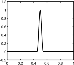
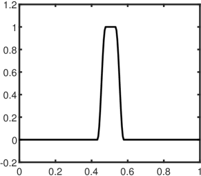
Figure 2: Left: Windowing function $W^{j}(x)$ (with $j=100$, on the domain $[0,1]$, and using $N=200$ discretization points) utilized in the definition of the windowed-localization operator $\Lambda$. Right: Windowing function $q_{18,9}(x-z)$ utilized for the localized filtering of the initial condition on the domain $[0,1]$ (using $N=200$ discretization points) for a discontinuity located at $z=0.5$.

The normalized windowing functions $\check{W}^{j}$ and the windowed-localization operator $\Lambda$, finally, are given by

$$\check{W}^{j}_{i}=\frac{W^{j}_{i}}{\sum_{k=0}^{N-1}W^{j}_{k}},$$ (35)

and

$$\Lambda[b]_{i}=\sum_{k=0}^{N-1}\check{W}^{k}_{i}b_{k},$$ (36)

respectively. Using these operators and functions, we define the 1D artificial viscosity operator

$$\tilde{\mu}[\textit{{e}}_{h}]_{i}=\Lambda[\widetilde{R}(\tilde{\tau}[\bm{\phi}])]_{i}\cdot\max_{j\in L^{i}}(\widetilde{S}[\textit{{e}}_{h}]_{j})h;$$ (37)

as mentioned in Section 1 and demonstrated in Section 4, use of the smooth artificial viscosity assignments produced by this expression yield smooth flows away from shocks and other discontinuities.

It is important to note the essential role of the windowed-localization operator in the assignment of smooth viscosity profiles. The smooth character of the resulting viscosity functions is illustrated in Figure 3, which showcases the viscosity assignments corresponding to the second time-step in the solution process. (This run corresponds to the Sod problem described in Section 4.3.1.) The left image displays the viscosity profiles used in [37] (which do not utilize the smoothing windows (36)) and the right image presents the window-based viscosity profile (37). The right-hand profile, which is comparable in size but, in fact, more sharply focused around the shock than the non-smooth profile on the left-hand image, helps eliminate spurious oscillations that otherwise arise from viscosity non-smoothness, and allows the FC-SDNN method to produce smooth flow fields, as demonstrated in Section 4.3.1.

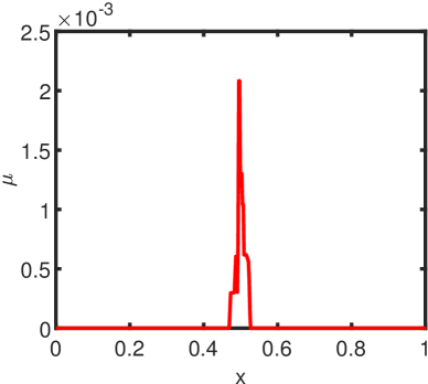
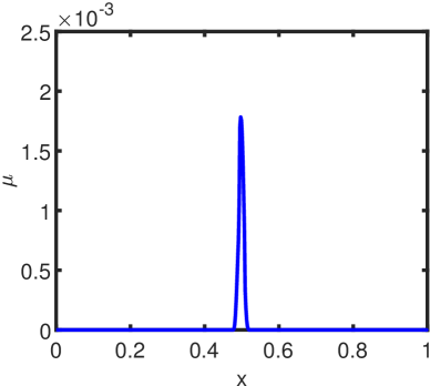
Figure 3: Comparison of the viscosity functions arising at the first viscous time-step for the Sod problem, using $N=500$ discretization points. Left: viscosity used in [37]. Right: viscosity used in the present FC-SDNN method (equation (37)).

Remark 3.

For the case of a 1D periodic problem, such as those considered in Section 4.1.2, the localization stencils and the windowing functions are defined by $L^{i}=\big{\{}x_{m(i-3,N)},\ldots,x_{m(i,N)},\ldots x_{m(i+3,N)}\big{\}}$, where the modulo function $m$ is defined in Section 3.2.1, and where $W^{j}_{i}=q_{c,r}(|x_{j}-x_{\widetilde{m}(i,j,N)}|)$. Here, for $s=\frac{c}{2}+r$ we have set

$$\widetilde{m}(i,j,N)=\left\{\begin{array}[]{ccc}j+N-i&\mbox{if}&j<2s\mbox{ and }N-2s+j\leq i\leq N-1\\ j-1-i&\mbox{if}&N-2s<j\leq N-1\mbox{ and }0\leq i\leq 2s-(N-j)\\ i&\mbox{else.}\\ \end{array}\right.$$ (38)

The values $c=0$ and $r=9$ considered previously are once again used in the periodic context.

As an example, Figure 4 displays the viscosity assignments produced, by the method described in this section for the function

$$u(x)=\left\{\begin{array}[]{cl}10(x-0.2)&\mbox{if }0.2<x\leq 0.3\\ 10(0.4-x)&\mbox{if }0.3<x\leq 0.4\\ 1&\mbox{if }0.6<x\leq 0.8\\ 100(x-1)(1.2-x)&\mbox{if }1<x\leq 1.2\\ 0&\mbox{otherwise.}\end{array}\right.$$ (39)

in the interval $[0,1.4]$. Clearly, the viscosity profiles are smooth and they are supported around points where the function $u$ is not smooth.

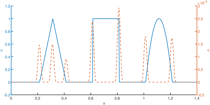
Figure 4: Viscosity assignment (orange dashed line) resulting from application of the SDNN-localized artificial viscosity algorithm to the initial condition (39) (blue solid line), using $N=500$ discretization points.

3.3.2 Two-dimensional case

The definition of the 2D viscosity operator follows similarly as the one for the 1D case, with adequately modified versions of the underlying functions and operators. In detail, in the present 2D case we define $\widetilde{R}$ and $R$ ($\widetilde{R}[\eta]_{ij}=R(\eta_{ij})$) as in the 1D case, but using the values $R(1)=1.5$, $R(2)=1$, $R(3)=0.5$, and $R(4)=0$. The $7\times 7$ localization stencils $L^{i,j}$ ($(i,j)\in\mathcal{I}$) are defined in terms of the 1D localization stencils $L^{i}$ and $L^{j}$ via the relation $L^{i,j}=L^{i}\times L^{j}$. For the 2D scalar Burgers equation, the MWSB operator $S[\textit{{e}}]$ (resp. the discrete operator $\widetilde{S}[\textit{{e}}_{h}]$) is taken to equal the maximum characteristic speed, that is $S[\textit{{e}}]=|u|$ (resp. $\widetilde{S}[\textit{{e}}_{h}]_{ij}=|u_{ij}|$ for $(i,j)\in\mathcal{I}$). In the case of the 2D Euler problem, the MWSB operator $S$ used in this paper assigns to e the upper bound $S(\textbf{{e}})=|u|+|v|+a$ on the speed of propagation $\mathbf{u}\cdot\vec{\kappa}+a$ of the wave corresponding to the largest eigenvalue of the 2D Flux-Jacobian (which, in a direction supported by the unit vector $\vec{\kappa}$, equals $\mathbf{u}\cdot\vec{\kappa}+a$ [15, Sec. 16.3 and 16.5]), so that the discrete operator $\widetilde{S}$ we propose is given on the grid by

$$\widetilde{S}[\textit{{e}}_{h}]_{ij}=|u_{ij}|+|v_{ij}|+a_{ij}.$$ (40)

Note that this MWSB operator, which equals $a$ plus the sum of the absolute values of the components of the velocity vector $\mathbf{u}$, differs slightly from the upper-bound selected in [13, 20], where the (equivalent) Euclidean-norm of $\mathbf{u}$ was used instead. The two-dimensional local-window operator, finally, is given by

$$\Lambda[b]_{ij}=\sum_{(k,\ell)\in\mathcal{I}}\check{W}^{k}_{i}\check{W}^{\ell}_{j}b_{k\ell}$$ (41)

—which, clearly, can be obtained in practice by applying consecutively the 1D local window operator introduced in Section 3.3.1 in the horizontal and vertical directions consecutively. As in the 1D case, using these operators and functions, we define the 2D artificial viscosity operator

$$\tilde{\mu}[\textit{{e}}_{h}]_{ij}=\Lambda[\widetilde{R}(\tilde{\tau}_{xy}[\bm{\phi}])]_{ij}\cdot\max_{(k,\ell)\in L^{ij}}(S[\textit{{e}}_{h}]_{k\ell})h.$$ (42)

3.4 Spectral filtering

Spectral methods regularly use filtering strategies in order to control the error growth in the unresolved high frequency modes. One such “global” filtering strategy is employed in the context of this paper as well, in conjunction with FC [1, 2], as detailed in Section 3.4.1. Additionally, a new “localized” filtering strategy 3.4.2 is introduced in this paper, in order to regularize discontinuous initial conditions, while avoiding the over-smearing of smooth flow-features. Details regarding the global and localized filtering strategies are provided in what follows.

3.4.1 Global filtering strategy

As indicated above, the proposed algorithm employs spectral filters in conjunction with the FC method to control the error growth in unresolved high frequency modes [1, 2]. For a given Fourier Continuation expansion

$$\sum_{k=-M}^{M}\hat{F}^{c}_{k}\exp(2\pi ikx/\beta)$$

the corresponding globally-filtered Fourier Continuation expansion is given by

$$\widetilde{F}_{g}=\sum_{k=-M}^{M}\hat{F}^{c}_{k}\sigma\Big{(}\frac{2k}{N+C}\Big{)}\exp(2\pi ikx/\beta)$$ (43)

where

$$\sigma\Big{(}\frac{2k}{N+C}\Big{)}=\exp\Big{(}-\alpha_{f}\Big{(}\frac{2k}{N+C}\Big{)}^{p_{f}}\Big{)}$$

for adequately chosen values of the positive integer $p_{f}$ and the real parameter $\alpha_{f}>0$. For applications involving two-dimensional domains the spectral filter is applied sequentially, one dimension at a time.

In the algorithm proposed in this paper, all the components of the unknown solution vector e are filtered using this procedure at every time step following the initial time, using the parameter values $\alpha_{f}=10$ and $p_{f}=14$, as indicated in Algorithm 1.

3.4.2 Localized discontinuity-smearing for initial data

In order to avoid the introduction of spurious oscillations arising from discontinuities in the initial condition, the spectral filter considered in the previous section is additionally applied, in a modified form, before the time-stepping process is initiated. A stronger filter is used to treat the initial conditions, however, since, unlike the flow field for positive times, the initial conditions are not affected by artificial viscosity. In order to avoid unduly degrading the representation of the smooth features of the initial data, on the other hand, a localized discontinuity-smearing method, based on use of filtering and windowing is used, that is described in what follows.

We first present the discontinuity-smearing approach for a 1D function $F:I\rightarrow\mathbb{R}$, defined on a one-dimensional interval $I$, which is discontinuous at a single point $z\in I$. In this case, the smeared-discontinuity function $\widetilde{F}_{\mathrm{sm}}$, which combines the globally filtered function $\widetilde{F}_{g}$ in a neighborhood of the discontinuity with the unfiltered function elsewhere, is defined by

$$\widetilde{F}_{\mathrm{sm}}(x)=q_{c,r}(x-z)\widetilde{F}_{g}(x)+(1-q_{c,r}(x-z))F(x),$$ (44)

Remark 4.

Throughout this paper, windows $q_{c,r}$ with $c=18$ and $r=9$ and globally filtered functions $\widetilde{F}_{g}$ with filter parameters $\alpha_{f}=10$ and $p_{f}=2$, which is depicted in Figure 2 right, were used for the initial-condition filtering problem, except as noted below in cases resulting in window overlap.

In case multiple discontinuities exist the procedure is repeated around each discontinuity point. Should the support of two or more of the associated windowing functions overlap, then each group of overlapping windows is replaced by a single window which equals zero outside the union of the supports of the windows in the group, and which equals one except in the rise regions for the leftmost and rightmost window functions in the group.

1:\\Initialization.

2:Input the trained ANN weights and biases (Section 3.2.2).

3:Initialize the unknown solution vector $\textit{{e}}_{h}$ (Section 2.1) to the given initial-condition values over the given spatial grid.

4:Initialize time: $t=0$.

5:while $t<T$ do

6:    Evaluate the proxy variable $\bm{\phi}$ corresponding to $\textit{{e}}_{h}$ at all spatial grid points.

7:    Obtain the smoothness classification values ($\tilde{\tau}[\bm{\phi}]$, equation (28), in the 1D case, or $\tilde{\tau}_{xy}[\bm{\phi}]$, equation (29), in the 2D case) at all grid points by applying steps (i) through (vi) in Section 3.2.1 as required in each case, 1D or 2D.

8:    Evaluate the MWSB operator $\widetilde{S}[\textit{{e}}_{h}]$ at all spatial grid points (Section 3.3.1 in the 1D cases, and Section 3.3.2 in the 2D cases).

9:    Determine the artificial viscosity assignments $\tilde{\mu}[\textit{{e}}_{h}]$ (Equation (37) in the 1D case or equation (42) in the 2D case) at all spatial grid points.

10:    (Case $t=0$) Apply localized discontinuity-smearing (Section 3.4.2) to the solution vector $\textit{{e}}_{h}$ and overwrite $\textit{{e}}_{h}$ with the resulting values.

11:    (Case $t>0$) Apply global filtering (Section 3.4.1) to the solution vector $\textit{{e}}_{h}$ and overwrite $\textit{{e}}_{h}$ with the resulting values.

12:    Evaluate the temporal step-size $\Delta t$ by substituting the discrete version $\widetilde{S}[\textit{{e}}_{h}]$ and $\tilde{\mu}[\textit{{e}}_{h}]$ of $S[\textit{{e}}]$ and $\mu[\textit{{e}}]$ in equation (22).

13:    Apply the SSPRK-4 time stepping scheme and FC-based spatial differentiation for given (Dirichlet or Neumann) boundary conditions (Sections 2.3 and 3.1) to the discrete version of the viscous system of equations (10)-(11) with $\mu[\textit{{e}}]$ substituted by $\tilde{\mu}[\textit{{e}}_{h}]$.

14:    Update time: $t=t+\Delta t$

15:end while

Algorithm 1 FC-SDNN algorithm

In the 2D case the localized filtering strategy is first performed along every horizontal line $y=y_{j:}$ for $0\leq j\leq N_{2}-1$. The resulting “partially” filtered function is then filtered along every vertical line $x=x_{i}$ for $0\leq i\leq N-1$ using the same procedure.

Remark 5.

For PDE problems involving vectorial unknowns, the localized discontinuity-smearing strategies for the initial condition is applied independently to each component.

As indicated in Algorithm 1, all the components of the initial ($t=0$) solution vector e are filtered using the procedure described in this section.

3.5 Algorithm pseudo-code

A pseudo-code for the complete FC-SDNN numerical method for the various equations considered in this paper, and for both 1D and 2D cases, is presented in Algorithm 1.

4 Numerical results

This section presents results of application of the FC-SDNN method to a number of non-periodic test problems (with the exception of a periodic linear-advection problem, in Section 4.1.2, demonstrating the limited dispersion of the method), time-dependent boundary conditions, shock waves impinging on physical boundaries (including a corner point and a non rectangular domain), etc. All of the examples presented in this section resulted from runs on Matlab implementations of the various methods used. Computing times are not reported in this paper in view of the inefficiencies associated with the interpreter computer language used but, for reference, we note from [38] that, for the types of equations considered in this paper, the FC implementations can be quite competitive, in terms of computing time, for a given accuracy. Our experiments indicate, further, that the relative cost of application of smooth-viscosity operators of the type used in this paper decreases as the mesh is refined, and that for large enough discretizations the relative cost of the neural network algorithm becomes insignificant. We thus expect that, as in [38], efficient implementations of the proposed FC-SDNN algorithm will prove highly competitive for general configurations.

4.1 Linear advection

The simple 1D linear-advection results presented in this section demonstrate, in a simple context, two main benefits resulting from the proposed approach, namely 1) Effective handling of boundary conditions (Section 4.1.1); and 2) Essentially dispersionless character (Section 4.1.2). For the examples in this section FC expansions with $d=5$ were used.

4.1.1 Boundary conditions

Figure 5 displays the FC-SDNN solution to the linear advection problem (2), in which three waves with various degrees of smoothness emanate from the left boundary, on the interval $[0,1.4]$ and with an initial condition $u(x,0)=0$ and boundary condition at $x=0$ given by

$$u(0,t)=\left\{\begin{array}[]{cl}100t(t-0.2)&\mbox{if }0<t<0.2\\ 1&\mbox{if }0.2<t<0.4\\ 10(t-0.8)&\mbox{if }0.8<t<0.9\\ 1-10(t-0.9)&\mbox{if }0.9<t<1\\ 0&\mbox{otherwise.}\end{array}\right.$$ (45)

At the outflow boundary $x=1.4$, the solution was evolved similarly as for the interior points. The solution was computed up to time $T=2$, using an adaptive time step given by (22), with $\textrm{CFL}=2$. As shown in Figure 5, the waves travel within the domain and match the position of the exact solution, showcasing the dispersionless character of the solver. The introduction of waves and irregularities at times $t=0$, $t=0.2$, $t=0.4$, $t=0.6$, $t=0.8$, $t=0.9$, $t=1$ through the left boundary is automatically accompanied by the assignment of artificial viscosity on a small area near that boundary. The FC-SDNN algorithm then stops assigning viscosity after a short time, when the irregularities are sufficiently smeared. This is a desirable property of the original algorithm [37] which is preserved in the present context. Finally, the waves exit the domain without producing undesired reflective artifacts around the boundary.

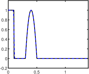
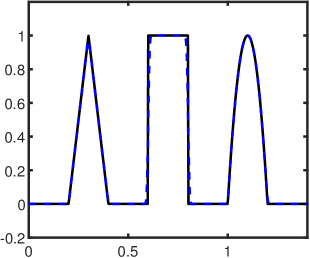
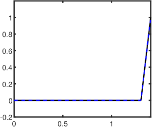
Figure 5: Solution of the non-periodic one dimensional linear advection problem at three different points in time, using $N=500$ discretization points. Exact (black solid line), FC-SDNN (blue dashed line). Left: $t=0.5$. Center: $t=1.3$. Right: $t=2.3$.

4.1.2 Limited dispersion

To demonstrate the limited dispersion inherent the FC-SDNN algorithm we consider a problem of cyclic advection of a “bump” solution over a bounded 1D spatial domain—thus effectively simulating, in a bounded domain, propagation over arbitrarily extended spatial regions. To do this we utilize the smooth cut-off “bump” function $\omega=\omega(x,q_{1},q_{2})$ ($q_{1}\neq q_{2}$) defined by

$$\omega(x,q_{1},q_{2})=\left\{\begin{array}[]{ccc}\exp(2\frac{e^{-1/\xi}}{\xi-1})&\mbox{if}&q_{1}\leq|x|\leq q_{2}\\ 1&\mbox{if}&|x|\leq q_{1}\\ 0&\mbox{if}&|x|\geq q_{2},\\ \end{array}\right.\quad\mbox{where}\quad\xi=\frac{|x|-q_{1}}{q_{2}-q_{1}}.$$ (46)

For this example we solve the equation (2) with $a=1$, starting from a smooth initial condition given by $u(x,0)=\omega(x-0.5,0,0.2)$, over the domain $\left[0,1\right]$ under periodic boundary conditions. In order to enforce such periodic conditions, the FC differentiation scheme is adapted, by using the same precomputed matrices $A_{\ell}$, $A_{r}$ and $Q$ (see Section 2.3) in conjunction with the ”wrapping” procedure described in [1, Sec. 3.3]. Using the FC-SDNN algorithm of order $d=5$ and SSPRK-4, the solution was evolved for five hundred periods, up to $T=500$; the resulting $t=500$ solution $u(x,500)$ is displayed in Figure 6. For comparison this figure presents numerical results obtained by means of a 6-th order central finite-difference scheme (also with SSPRK-4 time stepping). The finite-difference method uses a constant time-step $\Delta t=0.0034$, while the FC-SDNN uses the adaptive time step defined in (22) for which, in the present case, with $\mu=0$ and $S=1$, we have $\Delta t=0.0036$. Clearly, the FC-SDNN solution matches the exact solution remarkably well even after very long times, showcasing the low dissipation and dispersion afforded by the FC-based approach. In comparison, the higher-order finite difference solution suffers greatly from the dissipation and dispersion effects. Thus, significant advantages arise from use the FC-based strategy as well as the localized-viscosity approach that underlies the FC-SDNN method.

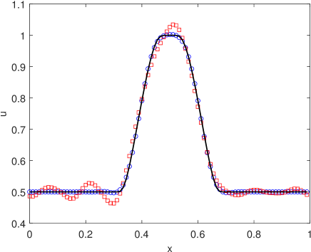
Figure 6: Numerical solutions to the periodic one-dimensional linear advection problem with $a=1$ up to time $T=500$: Exact solution (solid black line), fifth order FC-SDNN method (blue circles) and sixth order centered finite-difference scheme (red squares). Both numerical solutions were obtained using $N=90$ discretization points. In view of its nearly dispersionless character, the FC-based solution remains significantly more accurate than its higher order finite-difference counterpart.

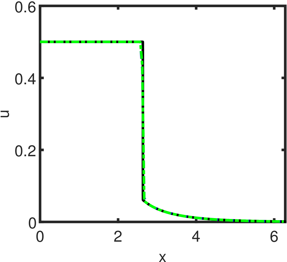
((a)) $t=2\pi$

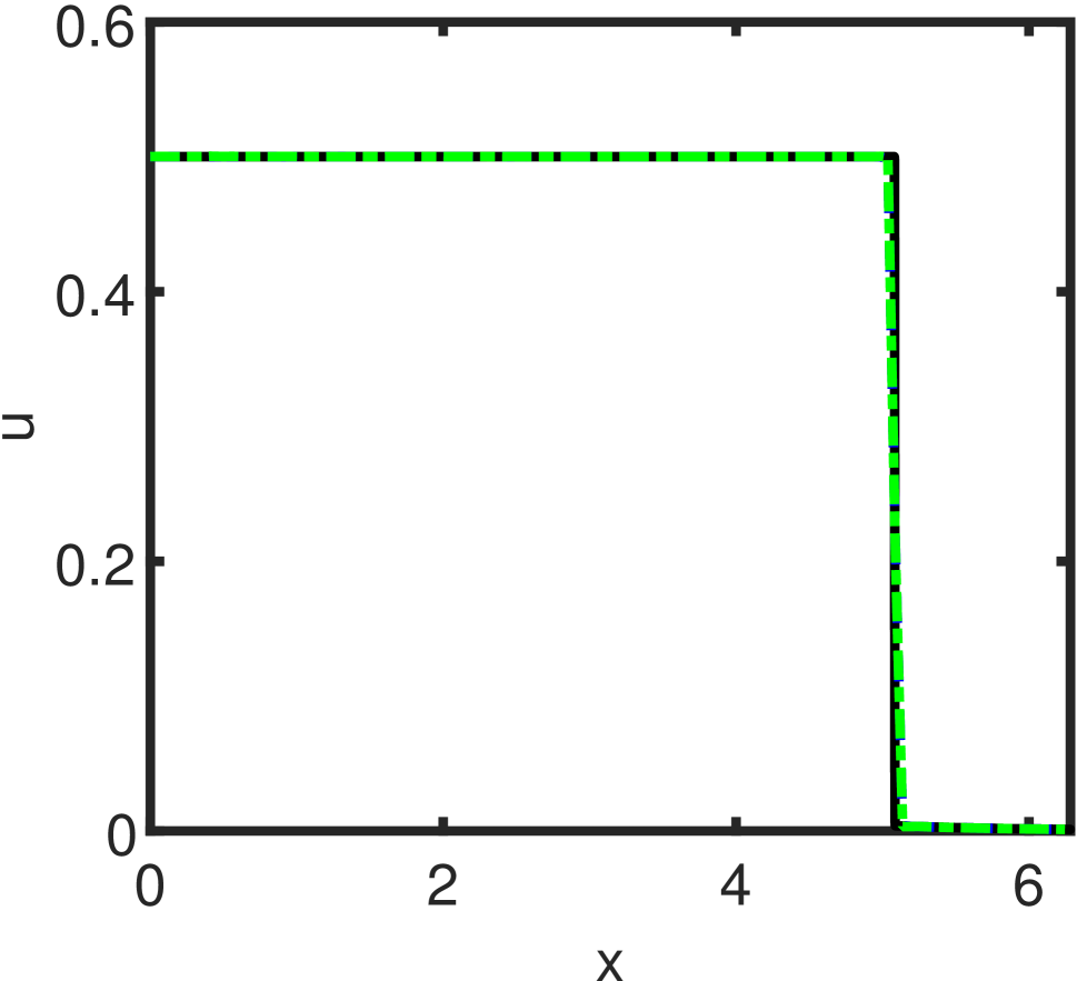
((b)) $t=5\pi$

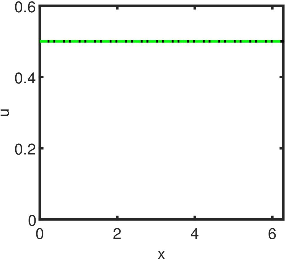
((c)) $t=8\pi$

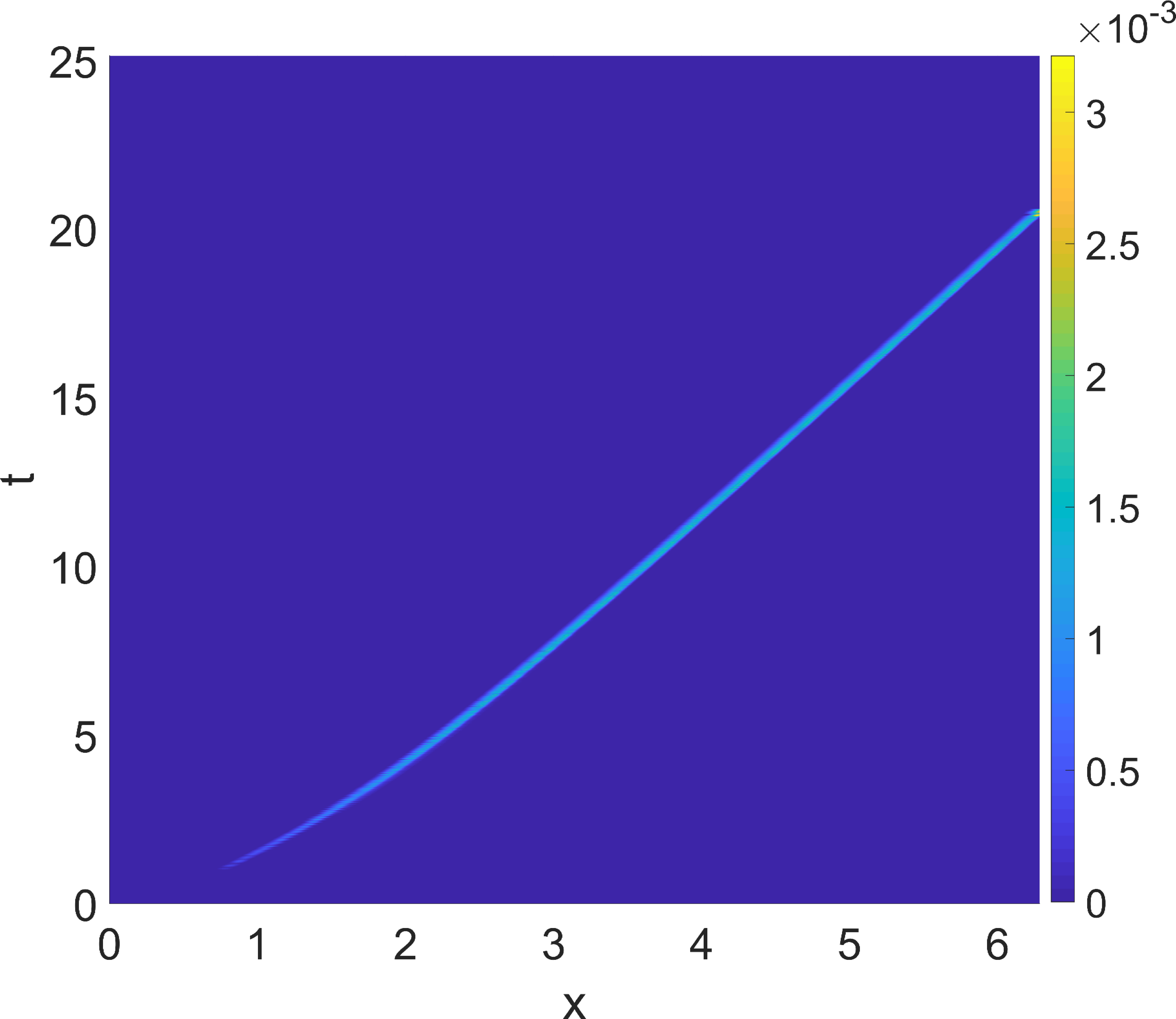
((d)) Time history of FC-SDNN artificial viscosity.

Figure 7: Solutions to the non-periodic one dimensional Burgers equation produced by the FC-SDNN and FC-EV algorithms of order $d=2$ at three different times $t$. Black solid line: finely resolved FC-SDNN ($N=10,000$, for reference). Blue dashed line: FC-SDNN with $N=500$. Green dot-dashed line: FC-EV with $N=500$.

4.2 Burgers equation

The 1D and 2D Burgers equation tests presented in this section demonstrate the FC-SDNN solver’s performance for simple nonlinear non-periodic problems. In particular, the 2D example showcases the ability of the algorithm to handle multi-dimensional problems where shocks intersect domain boundaries (a topic that is also considered in Section 4.3.2 in the context of the Euler equations).

4.2.1 1D Burgers equation

Figure 7 displays solutions to the 1D Burgers equation (3), where a shock forms from the sharp features in the initial condition

$$u_{0}(x)=\frac{1}{\exp(x-\frac{3}{20})[\tanh(10x-3)+1]-\tanh(10x-3)+1}.$$ (47)

Results of simulations produced by means of the FC-SDNN and FC-EV algorithms are presented in the figure. In both cases Dirichlet boundary conditions at the inflow boundary $x=0$ were used, while the solution at the outflow boundary $x=2\pi$ was evolved numerically in the same manner as the interior domain points. As shown in the figure, the shock is sharply resolved by both algorithms, with no visible oscillations. In both cases the shock eventually exits the physical domain without any undesired reflections or numerical artifacts. For this example FC expansions with $d=2$ were used. The reference solution (black) was computed on a 10000-point domain, with the FC-SDNN method.

4.2.2 2D Burgers equation

To demonstrate the solver’s performance and correct handling of shock-boundary interactions for 2D problems, we consider the 2D Burgers scalar equation (4) on the domain $\mathcal{D}=\left[0,1\right]\times\left[0,1\right]$, with an initial condition given by the function

$$u_{0}(x)=\left\{\begin{array}[]{ccc}-1&\mbox{if}&x\in[0.5,1]\mbox{ and }y\in[0.5,1]\\ -0.2&\mbox{if}&x\in[0,0.5]\mbox{ and }y\in[0.5,1]\\ 0.5&\mbox{if}&x\in[0,0.5]\mbox{ and }y\in[0,0.5]\\ 0.8&\mbox{if}&x\in[0.5,1]\mbox{ and }y\in[0,0.5],\end{array}\right.$$ (48)

and with vanishing normal derivatives at the boundary. This problem admits an explicit solution (displayed in Figure 8(b) at time $t=0.25$) which includes three shock waves and a rarefaction wave, all of which travel orthogonally to various straight boundary segments. Figures 8(c), 8(d), and 8(e) present the corresponding numerical solutions produced by the FC-SDNN algorithm at time $t=0.25$ resulting from use of various spatial discretizations and with adaptive time step given by (22) with $\textrm{CFL}=2$. Sharply resolved shock waves are clearly visible for the finer discretizations, as is the rarefaction wave in the lower part of the figure. The viscosity assignments, which are sharply concentrated near shock positions as the mesh is refined, suffice to avert the appearance of spurious oscillations. It is interesting to note that non-vanishing viscosity values are only assigned around shock discontinuities. (The SDNN algorithm assigns zero viscosity to the rarefaction wave for all time—as a result of the discontinuity-smearing introduced by the algorithm on the initial condition for the velocity, described in Section 3.4.2, which the FC-SDNN then preserves for all times in regions near the rarefaction wave on account of the resulting smoothness of the numerical solution in such regions). For this example FC expansions with $d=5$ were used.

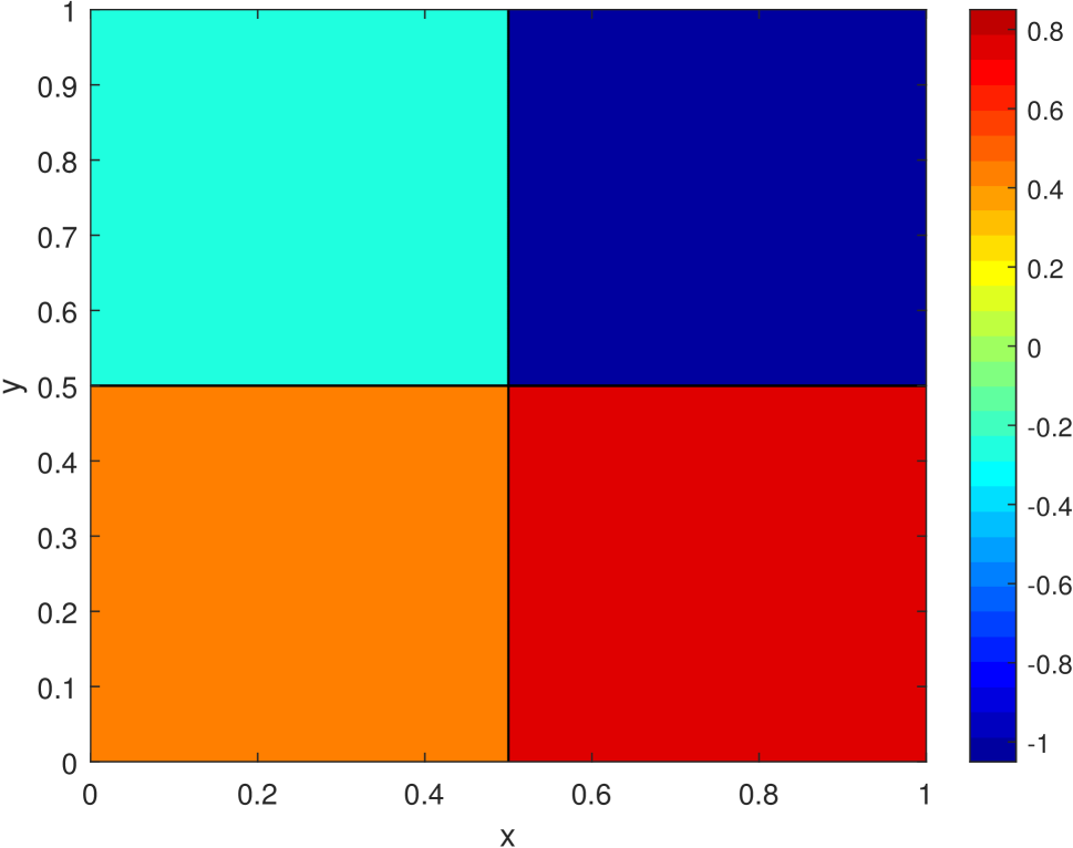
((a)) Initial condition

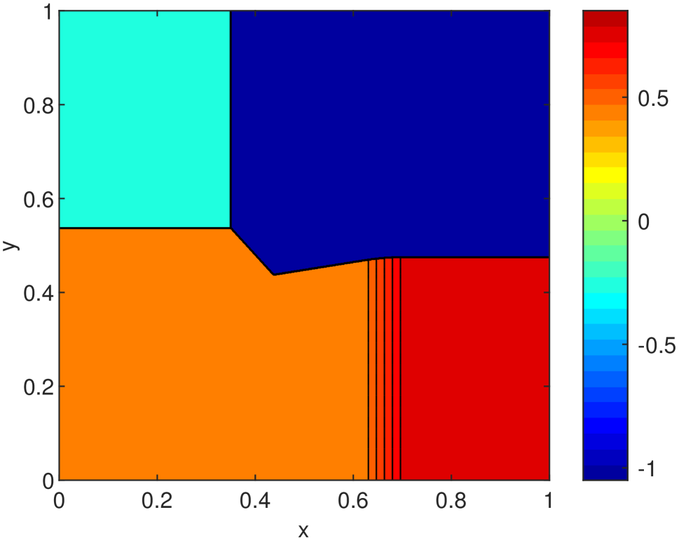
((b)) Exact solution

((c)) N = 200

((d)) N = 400

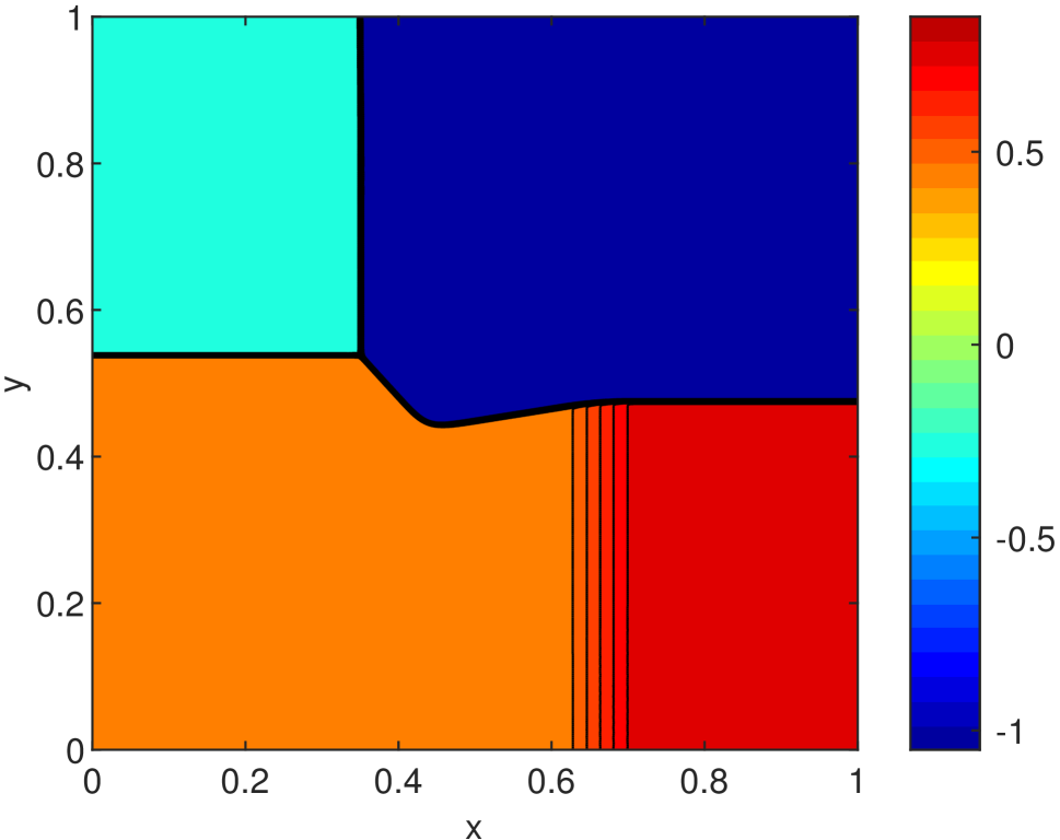
((e)) N = 1000

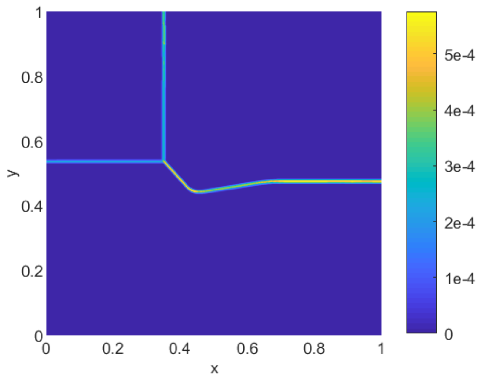
((f)) Art. visc. ($t=0.25$, $N=1000$)

.

Figure 8: Fifth-order ($d=5$) FC-SDNN numerical solution to the 2D Burgers equation with initial condition displayed on the upper-left panel, whose exact solution at $t=0.25$ is displayed on the upper-right panel. The middle and left-lower panels display the FC-SDNN numerical solutions at $t=0.25$ obtained by using $N\times N$ spatial grids with three different values of $N$, as indicated in each panel. The FC-SDNN numerical viscosity at $t=0.25$ for the case $N=1000$ is presented in the lower-right panel.

4.3 1D and 2D Euler systems

This section presents a range of 1D and 2D test cases for the Euler system demonstrating the FC-SDNN algorithm’s performance in the context of a nonlinear systems of equations. The test cases include well-known 2D arrangements, including the shock-vortex interaction example [39], 2D Riemann problem flow [24], Mach 3 forward facing step [45], and Double Mach reflection [45]. In particular the results illustrate the algorithm’s ability to handle contact discontinuities and shock-shock interactions as well as shock reflection and propagation along physical and computational boundaries.

4.3.1 1D Euler problems

The 1D shock-tube tests considered in this section demonstrate the solver’s ability to capture not only shock-wave discontinuities (that also occur in the Burgers test examples considered in Section 4.2) but also contact discontinuities. Fortunately, in view of the localized spectral filtering strategy used for the initial-data (Section 3.4.2), the algorithm completely avoids the use of artificial viscosity around contact discontinuities, and thus leads to excellent resolution of these important flow features. This is demonstrated in a variety of well known test cases, including the Sod [41], Lax [23], Shu-Osher [40] and Blast Wave [34] problems, with flows going from left to right—so that the left boundary point (resp. right boundary point) is the inflow (resp. outflow) boundary. In all cases an adaptive time step given by (22) with $\textrm{CFL}=2$ was used, and, following [15, Sec. 19], inflow (resp. outflow) boundary condition were enforced at the inflow boundaries (resp. outflow boundaries) by setting $\rho$ and $u$ (resp $p$) identically equal, for all time, to the corresponding boundary values of these quantities at the initial time $t=0$. For the examples in this section FC expansions with $d=5$ were used.

Sod problem.

We consider a Sod shock-tube problem for the 1D Euler equations (5) on the interval $[-4,5]$ with initial conditions

$$(\rho,u,p)=\left\{\begin{array}[]{ccc}(1,0,1)&\mbox{if}&x<0.5\\ (0.125,0,0.1)&\mbox{if}&x>0.5,\\ \end{array}\right.$$

a setup that gives rise (from right to left) to a right-moving shock wave, a contact discontinuity and a rarefaction wave (upper and middle left images in Figure 9). The solution was computed up to time $T=2$. The results presented in Figure 9 show well resolved shocks (upper and middle right) and contact discontinuities (upper and middle center), with no visible Gibbs oscillations in any case. The FC-SDNN and FC-EV solvers demonstrate a similar resolution in a vicinity of the shock, but the FC-SDNN method provides a much sharper resolution of the contact-discontinuity. As shown in Figure (9(c)), after a short time the FC-SDNN algorithm does not assign artificial viscosity in a vicinity of the contact discontinuity, leading to the significantly more accurate resolution observed for this flow feature.

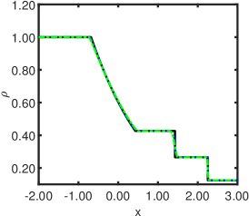
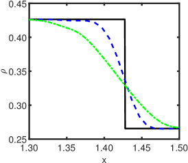
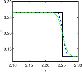
((a)) N = 500

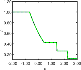
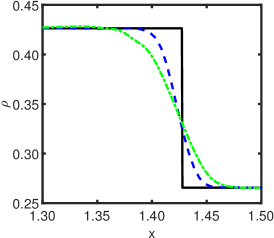
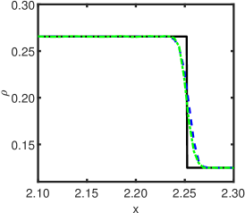
((b)) N = 1000

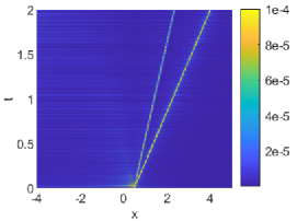
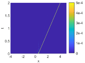
((c)) Time history of assigned artificial viscosity for N = 1000, for FC-EV (left) and FC-SDNN (right).

Figure 9: Solutions to the Sod problem produced by the FC-SDNN and FC-EV algorithms of order $d=5$ at $t=0.2$. Exact solution: solid black line. FC-SDNN solution: Blue dashed-line. FC-EV solution: Green dot-dashed line. Numbers of discretization points: $N=500$ in the upper panels and $N=1000$ in the middle panels. Bottom panels: artificial viscosity assignments.

Lax problem.

We consider a Lax problem on the interval $[-5,5]$, with initial condition

$$(\rho,u,p)=\left\{\begin{array}[]{ccc}(0.445,0.698,3.528)&\mbox{if}&x<0\\ (0.5,0,0.571)&\mbox{if}&x>0\\ \end{array}\right.$$

which results in a combination (from right to left) of a shock wave, a contact discontinuity and a rarefaction wave (upper and middle left images in Figure 10). The solution was computed up to time $T=1.3$. The results are presented in Figure 10, which shows well resolved shocks (upper and middle right) without detectable Gibbs oscillations. The viscosity time history displayed in Figure 10(c) shows that the FC-SDNN method only assigns artificial viscosity in the vicinity of the shock discontinuity but, as discussed above, not around the contact discontinuity, leading to a sharper resolution by the FC-SDNN method in this region (upper and middle center). The shock resolution is similar for the EV and SDNN algorithms, but the latter approach is significantly more accurate around the contact discontinuity.

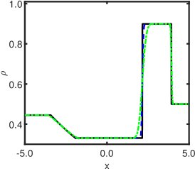
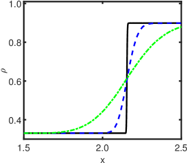
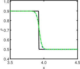
((a)) N = 500

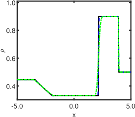
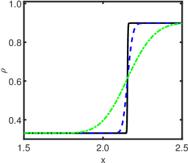
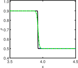
((b)) N = 1000

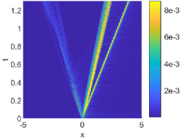
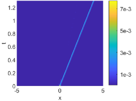
((c)) Time history of assigned artificial viscosity for N = 1000, for FC-EV (left) and FC-SDNN (right).

Figure 10: Solutions to the Lax problem produced by the FC-SDNN and FC-EV algorithms of order $d=5$ at $t=1.3$. Exact solution: solid black line. FC-SDNN solution: Blue dashed-line. FC-EV solution: Green dot-dashed line. Numbers of discretization points: $N=500$ in the upper panels and $N=1000$ in the middle panels. Bottom panels: artificial viscosity assignments.

Shu-Osher problem.

We consider the Shu-Osher shock-entropy problem on the interval $[-5,5]$, with initial condition given by

$$(\rho,u,p)=\left\{\begin{array}[]{ccc}(3.857143,2.6929369,10.33333)&\mbox{if}&x<-4\\ (1+0.2\text{sin}(5x),0,1)&\mbox{if}&x>-4.\\ \end{array}\right.$$ (49)

The solution is computed up to time $T=1.8$. In this problem, a shock wave encounters an oscillatory smooth wavetrain. This test highlights the FC-SDNN solver’s low dissipation, as artificial viscosity is only assigned in the vicinity of the right-traveling shock as long as the waves remain smooth, allowing for an accurate representation of the smooth features. In particular, Figure (11(c)) shows that the support of the FC-SDNN artificial viscosity is much more narrowly confined around the shock position than the artificial viscosity resulting in the FC-EV approach. As a result, and as illustrated in Figure (11) (upper and middle right images), the FC-SDNN method provides a more accurate resolution in the acoustic region (behind the main, rightmost, shock).

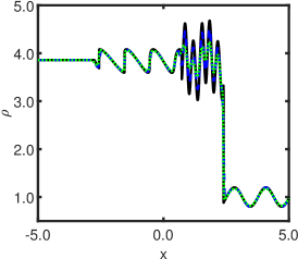
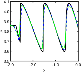
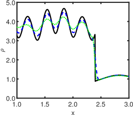
((a)) N = 500

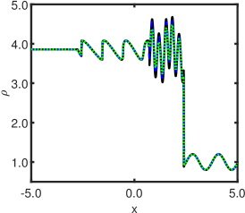
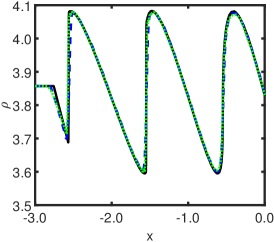
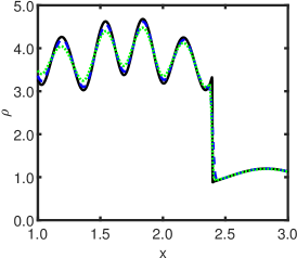
((b)) N = 1000

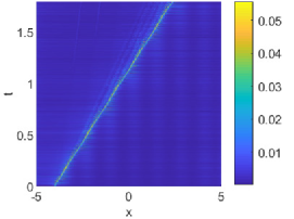
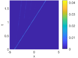
((c)) Time history of assigned artificial viscosity for N = 1000, for FC-EV (left) and FC-SDNN (right).

Figure 11: Solutions to the Shu-Osher problem produced by the FC-SDNN and FC-EV algorithms of order $d=5$ at $t=1.8$. Solid black line: finely resolved FC-SDNN ($N=10,000$, for reference). Blue dashed line: FC-SDNN with $N=500$ and $N=1000$ (middle panels). Green dot-dashed line: FC-EV with $N=500$ (upper panels) and $N=1000$ (middle panels). Bottom panels: artificial viscosity assignments.

Blast Wave problem.

Finally, we consider the Blast Wave problem as presented in [34], on the interval $[0,1]$, with initial conditions given by

$$(\rho,u,p)=\left\{\begin{array}[]{ccc}(1,0,1000)&\mbox{if}&x<0.5\\ (1,0,0.01)&\mbox{if}&x>0.5,\\ \end{array}\right.$$ (50)

up to time $T=0.012$. This setup is similar to the one considered in the Sod problem, but with a much stronger right-moving shock. In order to avoid unphysical oscillations at the boundaries, which could result from the presence of the strong shock, the value of the operator $\tau$ is set to $1$ on the leftmost and rightmost nine points in the domain, thus effectively assigning a small amount of viscosity at the boundaries at every time step of the simulation. As shown in Figure 12, the shock is sharply resolved by both the FC-SDNN and FC-EV approaches. As the mesh is refined the contact discontinuity is resolved more sharply by the former method which, as in the previous examples, does not assign viscosity around such features.

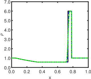
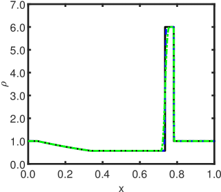
((a)) ”wide”

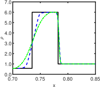
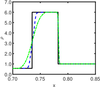
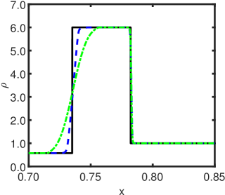
((b)) ”zoom”

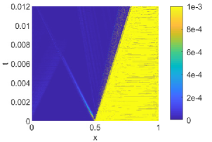
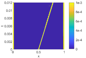
((c)) Time history of assigned artificial viscosity for $N=1000$, for FC-EV (left) and FC-SDNN (right).

Figure 12: Solutions to the Blast wave problem produced by the FC-SDNN and FC-EV algorithms of order $d=5$ at $t=0.012$. Solid black line: exact solution. Blue dashed line: FC-SDNN with $N=1000$ (upper- and middle-left panels), $N=2000$ (upper- and middle-center panels), and $N=3000$ (upper- and middle-right panels). Green dot-dashed line: FC-EV with $N=1000$ (left panels), $N=2000$ (center panels), and $N=3000$ (right panels). Bottom panels: artificial viscosity assignments.

4.3.2 2D Euler problems

The test cases considered in this section showcase the FC-SDNN method’s ability to handle complex shock-shock, as well as shock-boundary interactions, including shocks moving orthogonally to the boundaries as in the Riemann 2D and the Shock vortex problems, or moving obliquely to the boundary of the domain, after reflecting on a solid wedge, in the Double Mach reflection problem, or reflecting multiple times on the solid walls of a wind tunnel with a step, in the Mach 3 forward facing step problem. For the examples in this section FC expansions with $d=2$ were used. As a result the FC method can provide significantly improved accuracy over other approaches of the same or even higher accuracy orders. In all cases the solutions obtained are in agreement with solutions obtained previously by various methods [45, 24, 13, 29]. As indicated in the introduction, the proposed approach leads to smooth flows away from shocks, as evidenced by correspondingly smooth level set lines for the various flow quantities, in contrast with corresponding results provided by previous methods.

Riemann problem (Configuration 4 in [24]).

We consider a Riemann problem configuration on the domain $[0,1.2]\times[0,1.2]$, with initial conditions given by

$$(\rho,u,v,p)=\left\{\begin{array}[]{ccc}(1.1,0,0,1.1)&\mbox{if}&x\in[0.6,1.2]\mbox{ and }y\in[0.6,1.2]\\ (0.5065,0.8939,0,0.35)&\mbox{if}&x\in[0,0.6)\mbox{ and }y\in[0.6,1.2]\\ (1.1,0.8939,0,0.35)&\mbox{if}&x\in[0,0.6)\mbox{ and }y\in[0,0.6)\\ (0.5065,0,0.8939,0.35)&\mbox{if}&x\in[0.6,1.2]\mbox{ and }y\in[0,0.6),\end{array}\right.$$ (51)

and with vanishing normal derivatives for all variables on the boundary, at all times. The solution is computed up to time $T=0.25$ by means of the FC-SDNN approach. The initial setting induces four interacting shock waves, all of which travel orthogonally to the straight segments of the domain boundary. The results, presented in Figure 13, show a sharpening of the shocks as the mesh is refined and an absence of spurious oscillations in all cases. As shown on the left image in Figure 14, the FC-SDNN viscosity assignments are sharply concentrated near the shock positions.

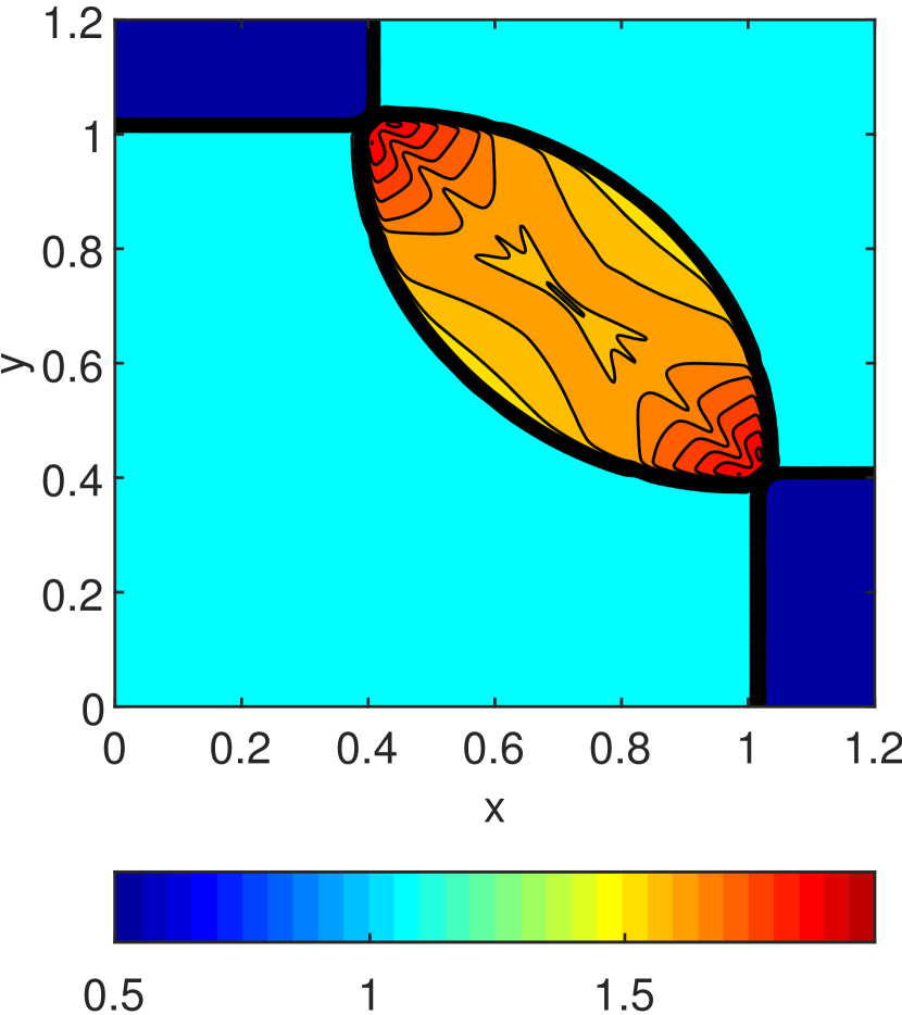
((a)) N = 400

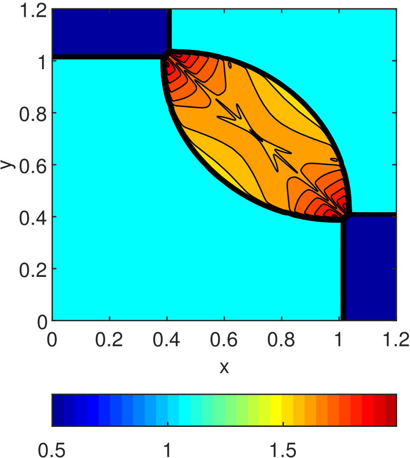
((b)) N = 600

((c)) N = 800

Figure 13: Second-order ($d=2$) FC-SDNN numerical solution to the Euler 2D Riemann problem considered in Section 4.3.2, at $t=0.25$, obtained by using a spatial discretization containing $N\times N$ grid points with three different values of $N$, as indicated in each panel. For each discretization, the solution is represented using thirty equispaced contours between $\rho=0.5$ and $\rho=1.99$.

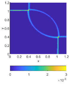
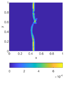
Figure 14: Artificial viscosity profiles for the Euler 2D Riemann problem considered in Figure 13 at $t=0.25$ (left) and for the Shock vortex problem considered in Figure 15 at $t=0.35$ (right).

Shock vortex problem [39].

We next consider a “shock-vortex” problem in the domain $[0,1]\times[0,1]$, in which a shock wave collides with an isentropic vortex. The initial conditions are given by

$$(\rho,u,v,p)=\left\{\begin{array}[]{ccc}(\rho_{L}+\tilde{\rho},u_{L}+\tilde{u},v_{L}+\tilde{v},p_{L}+\tilde{p})&\mbox{if}&x\in[0,0.5)\\ (\rho_{R},u_{R},v_{R},p_{R})&\mbox{if}&x\in[0.5,1]\end{array}\right.$$ (52)

where the left state equals the combination of the unperturbed left-state $(\rho_{L},u_{L},v_{L},p_{L})=(1,\sqrt{\gamma},0,1)$ in the shock wave with the isentropic vortex

$$\tilde{u}=\frac{x-x_{c}}{r_{c}}\Phi(r),\quad\tilde{v}=-\frac{x-x_{c}}{r_{c}}\Phi(r),\quad\frac{\gamma-1}{4\zeta\gamma}\Phi(r)^{2}=\frac{p_{L}}{\rho_{L}}-\frac{p_{L}+\tilde{p}}{\rho_{L}+\tilde{\rho}},\quad p_{L}+\tilde{p}=(\rho_{L}+\tilde{\rho})^{\gamma},$$ (53)

centered at $(x_{c},y_{c})=(0.25,0.5)$ (where $r=\sqrt{(x-x_{c})^{2}+(y-y_{c})^{2}}$, $\Phi(r)=\epsilon e^{\zeta(1-(r/r_{c})^{2})}$). As in previous references for this example we use the vortex parameter values $r_{c}=0.05$, $\zeta=0.204$, and $\epsilon=0.3$. The initial right state is given by

$$\rho_{R}=\rho_{L}\frac{(\gamma+1)p_{R}+\gamma-1}{(\gamma-1)p_{R}+\gamma+1},\quad u_{R}=\sqrt{\gamma}+\sqrt{2}\frac{1-p_{R}}{\sqrt{\gamma-1+p_{R}(\gamma-1)}},\quad v_{R}=0,\quad p_{R}=1.3.$$

Vanishing normal derivatives for all variables were imposed on the domain boundary at all times.

The solution was obtained up to time $T=0.35$, for which the vortex has completely crossed the shock. The solutions displayed in Figure 15 demonstrate the convergence of the method as the spatial and temporal discretizations are refined: shocks become sharper with each mesh refinement, while the vortex features remain smooth after the collision with the shock wave—a property that other solvers do not enjoy, and which provides an indicator of the quality of the solution. The right image in Figure 14 shows that, as in the previous examples, the support of the artificial viscosity imposed by the SDNN algorithm is narrowly focused in a vicinity of the shock.

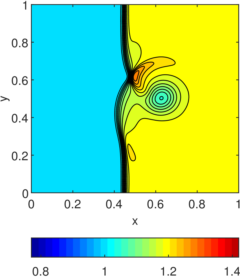
((a)) N = 200

((b)) N = 300

((c)) N = 400

Figure 15: Second-order ($d=2$) FC-SDNN numerical solution to the Euler 2D Shock-vortex problem considered in Section 4.3.2, at $t=0.35$, obtained by using a spatial discretization containing $N\times N$ grid points with three different values of $N$, as indicated in each panel. For each discretization, the solution is represented using thirty equispaced contours between $\rho=0.77$ and $\rho=1.42$.

Mach 3 forward facing step [45].

We now consider a “Mach 3 forward facing step problem” on the domain $([0,0.6]\times[0,1])\cup([0.6,3]\times[0.2,1])$, in which a uniform Mach 3 flow streams through a wind tunnel with a forward facing step, of 0.2 units in height, located at $x=0.6$. The initial condition is given by

$$(\rho,u,v,p)=\left\{\begin{array}[]{ccc}(1.4,3,0,1)&\mbox{if}&(x,y)\in([0,0.6)\times[0,1])\cup([0.6,3]\times[0.2,1])\\ (1.4,0,0,1)&\mbox{if}&(x,y)\in\{0.6\}\times[0,0.2],\end{array}\right.$$ (54)

and the solution is computed up to time $T=4$. An inflow condition is imposed at the left boundary at all times which coincides with the initial values on that boundary, while the equations are evolved at the outflow right boundary. Reflecting boundary conditions (zero normal velocity) are applied at all the other boundaries. (Following [45, 13], no boundary condition is enforced at the node located at the step corner.) The simulation was performed using the adaptive time step (22) with $\textrm{CFL}=1$. The density solution is displayed in Figure 16.

Double Mach reflection [45]

We finally consider the “Double Mach reflection problem” on the domain $[0,4]\times[0,1]$. This problem contains a reflective wall located on the $x\geq x_{r}$ part of the bottom boundary $y=0$ (here we take $x_{r}=1/6$), upon which there impinges an incoming shock wave forming a $\theta=\pi/3$ angle with the positive $x$-axis. The initial condition is given by

$$\mathbf{e}(x,y,0)=(\rho,\rho u,\rho v,E)=\left\{\begin{array}[]{ccc}(8,57.1597,-33.0012,563.544)&\mbox{if}&0\leq x\leq x_{r}+\frac{y}{\sin(\theta)}\\ (1.4,0,0,2.5)&\mbox{if}&x_{r}+\frac{y}{\sin(\theta)}\leq x\leq 4\end{array}\right.$$ (55)

and the solution is computed up to time $T=0.2$. This setup, introduced in [45], gives rise to the reflection of a strong oblique shock wave on a wall. (Equivalently, upon counter-clockwise rotation by $30^{\circ}$, this setup can be interpreted as a vertical shock impinging on a $30^{\circ}$ ramp.) As a result of the shock reflection a number of flow features arise, including, notably, two Mach stems and two contact discontinuities (slip lines), as further discussed below in this section.

The initial and boundary values used in this context do not exactly coincide with the ones utilized in [45]. Indeed, on one hand, in order to avoid density oscillations near the intersection of the shock and the top computational boundary, we utilize “oblique” Neumann boundary conditions on all flow variables $\mathbf{e}=(\rho,\rho u,\rho v,E)$. More precisely, we enforce zero values on the derivative of $\mathbf{e}$ with respect to the direction parallel to the shock, along both the complete upper computational boundary and the region $0\leq x\leq x_{r}$ (that is, left of the ramp) on the lower computational boundary. This method can be considered as a further development of the approach proposed in [43], wherein an extended domain in the oblique direction was utilized in conjunction with Neumann conditions along the normal direction to the oblique boundary. In order to incorporate the oblique Neumann boundary condition we utilized the method described in [2], which, in the present application, proceeds by obtaining relations between oblique, normal and tangential derivatives of the flow variables $\mathbf{e}$. Inflow boundary conditions were used which prescribe time-independent values of $\rho$, $u$ and $v$ on the left boundary; outflow conditions on the right boundary, in turn, enforce a time independent value of $p$.

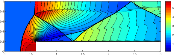
((a)) Thirty equispaced $\rho$ contours between 0.18 and 5.71

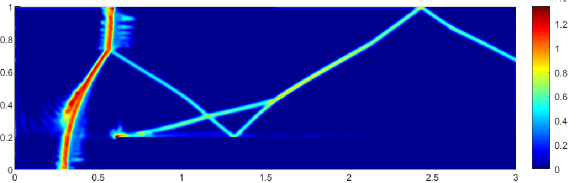
((b)) Artificial viscosity at time t=4.

Figure 16: Top panel: Second-order ($d=2$) FC-SDNN numerical solution to the Mach 3 forward facing-step problem considered in Section 4.3.2, at $t=4$, obtained by using $1200\times 400$ spatial grid. Bottom panel: Viscosity assignment.

Additionally, following [43], we utilize a numerical viscous incident shock as an initial condition in order to avoid well-known post-shock oscillations, as noted in [17], that result from the use of a sharp initial profile. Such a smeared shock is obtained in our context by applying the FC-SDNN solver to the propagation of an oblique flat shock on all of space (without the ramp) up to time $T=0.2$, including imposition of oblique Neumann boundary conditions throughout the top and bottom boundary. The solution $\hat{\mathbf{e}}_{h}$ amounts to a smeared shock profile on the $(x,y)$ plane which, at time $t$, is centered on the straight line $x=x_{s}(y,t)$ where $x_{s}(y,t)=x_{r}+\frac{U_{s}}{\sin(\theta)}t+\frac{y}{\tan(\theta)}$. This shock is followed by some back-trailing oscillations, as has been observed in [17, 43]. In order to eliminate these artifacts from the initial condition, a diagonal strip of $N_{d}$ points centered around the shock location is selected. Then, on a strip of $N_{d}$ points surrounding the initial position of the shock, the initial condition $\mathbf{e}_{h}$ to the Double Mach reflection problem is defined as

$$\mathbf{e}_{h}(x,y,0)=q_{c,r}(x_{s}(y,0)-x)\hat{\mathbf{e}}_{h}(x+x_{s}(y,T),y,T)+(1-q_{c,r}(x_{s}(y,0)-x))\mathbf{e}(x,y,0)$$

where $q_{c,r}$ is the window function defined in (34). $N_{d}$ is taken to be small enough to exclude the back-trailing oscillations from the strip, and large enough as to provide a relatively smooth profile for the initial condition. For the double-Mach solution depicted in Figure 17, which was obtained on the basis of a $3200\times 800$-point grid, the incident-shock parameter values $N_{d}=125$, $c=25$ and $r=50$ were used.

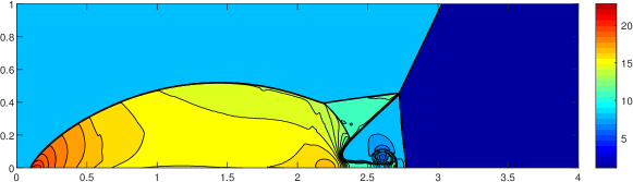
((a)) Thirty equispaced $\rho$ contours between 1.0 and 22.8

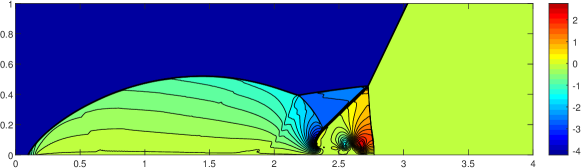
((b)) Thirty equispaced $v$ contours between -4.2 and 2.7

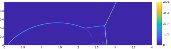
((c)) Artificial viscosity at time $t=0.2$

Figure 17: Top and middle panels: Second-order ($d=2$) FC-SDNN numerical solution to the Double Mach reflection problem considered in Section 4.3.2, at $t=0.2$, obtained by using $3200\times 800$ spatial grid. Bottom panel: Viscosity assignment.

Among several notable features in the $t=0.2$ solution we mention the density-contour roll-ups of the primary slip line that are clearly visible in the density component of the solution presented in Figure 17a near the reflective wall around $x=2.6$, as well as the extremely weak secondary slip line, that is most easily noticeable in the variable $v$ (Figure 17b) as a dip in the contour lines within the rectangle $[1.9,2.2]\times[0,0.4]$, but which is also visible in this area as a blip in the density contour lines (Figure 17a). The accurate simulation of these two features has typically been found challenging [45, 18, 43]. The elimination of back-trailing shock oscillations, which was accomplished, as discussed above, by resorting to use of a numerically viscous incident shock, is instrumental in the resolution of the secondary slip line—which might otherwise be polluted by such oscillations to the point of being unrecognizable.

5 Conclusions

This paper introduced the FC-SDNN method, a neural network-based artificial viscosity method for evaluation of shock dynamics in non-periodic domains. In smooth flow areas the method enjoys the essentially dispersionless character inherent in the FC method. The smooth but localized viscosity assignments allow for a sharp resolution of shocks and contact discontinuities, while yielding smooth flow profiles away from jump discontinuities. An efficient implementation for general 2D and 3D domains, which could be pursued on the basis of an overlapping-patch setup [1, 3], is left for future work.

Acknowledgments. OB and DL gratefully acknowledges support from NSF under contracts DMS-1714169 and DMS-2109831, from AFOSR under contract FA9550-21-1-0373, and from the NSSEFF Vannevar Bush Fellowship under contract number N00014-16-1-2808. Initial conversations with J. Paul are gratefully acknowledged.

References

- [1] N. Albin and O. P. Bruno. A spectral FC solver for the compressible Navier–Stokes equations in general domains I: Explicit time-stepping. Journal of Computational Physics, 230:6248–6270, 2011.
- [2] F. Amlani and O. P. Bruno. An FC-based spectral solver for elastodynamic problems in general three-dimensional domains. Journal of Computational Physics, 307:333–354, 2016.
- [3] D. L. Brown, W. D. Henshaw, and D. J. Quinlan. Overture: An object-oriented framework for solving partial differential equations. In International Conference on Computing in Object-Oriented Parallel Environments, pages 177–184. Springer, 1997.
- [4] O. P. Bruno, M. Cubillos, and E. Jimenez. Higher-order implicit-explicit multi-domain compressible Navier-Stokes solvers. Journal of Computational Physics, 391:322–346, 2019.
- [5] O. P. Bruno and M. Lyon. High-order unconditionally stable FC-AD solvers for general smooth domains I. Basic elements. Journal of Computational Physics, 229(6):2009–2033, 2010.
- [6] O. P. Bruno and J. Paul. Two-dimensional Fourier Continuation and applications. arXiv:2010.03901, 2020.
- [7] M. H. Carpenter, D. Gottlieb, S. Abarbanel, and W.-S. Don. The theoretical accuracy of Runge–Kutta time discretizations for the initial boundary value problem: a study of the boundary error. SIAM Journal on Scientific Computing, 16(6):1241–1252, 1995.
- [8] N. Discacciati, J. S. Hesthaven, and D. Ray. Controlling oscillations in high-order Discontinuous Galerkin schemes using artificial viscosity tuned by neural networks. Journal of Computational Physics, 409:109304, 2020.
- [9] R. A. Gentry, R. E. Martin, and B. J. Daly. An Eulerian differencing method for unsteady compressible flow problems. Journal of Computational Physics, 1(1):87–118, 1966.
- [10] X. Glorot and Y. Bengio. Understanding the difficulty of training deep feedforward neural networks. In JMLR Workshop and Conference Proceedings, pages 249–256, 2010.
- [11] I. Goodfellow, Y. Bengio, and A. Courville. Deep Learning. MIT Press, 2016.
- [12] S. Gottlieb. On high order strong stability preserving Runge-Kutta and multi step time discretizations. Journal of Scientific Computing, 25(1):105–128, 2005.
- [13] J.-L. Guermond, R. Pasquetti, and B. Popov. Entropy viscosity method for nonlinear conservation laws. Journal of Computational Physics, 230(11):4248–4267, 2011.
- [14] A. Harten, B. Engquist, S. Osher, and S. R. Chakravarthy. Uniformly high order accurate essentially non-oscillatory schemes, III. In Upwind and high-resolution schemes, pages 218–290. Springer, 1987.
- [15] C. Hirsch. Numerical computation of internal and external flows. Vol. 2-Computational methods for inviscid and viscous flows. John Wiley & Sons, 1990, 708, 1990.
- [16] G.-S. Jiang and C.-W. Shu. Efficient implementation of weighted ENO schemes. Journal of Computational Physics, 126(1):202–228, 1996.
- [17] E. Johnsen and S. Lele. Numerical errors generated in simulations of slowly moving shocks. Center for Turbulence Research, Annual Research Briefs, pages 1–12, 2008.
- [18] F. Kemm. On the proper setup of the double Mach reflection as a test case for the resolution of gas dynamics codes. Computers & Fluids, 132:72–75, 2016.
- [19] D. A. Kopriva. Implementing spectral methods for partial differential equations: Algorithms for scientists and engineers. Springer Science & Business Media, 2009.
- [20] A. Kornelus and D. Appelö. Flux-conservative Hermite methods for simulation of nonlinear conservation laws. Journal of Scientific Computing, 76(1):24–47, 2018.
- [21] A. Lapidus. A detached shock calculation by second-order finite differences. Journal of Computational Physics, 2(2):154–177, 1967.
- [22] P. Lax. Systems of conservation laws. Technical report, LOS ALAMOS NATIONAL LAB NM, 1959.
- [23] P. D. Lax. Weak solutions of nonlinear hyperbolic equations and their numerical computation. Communications on pure and applied mathematics, 7(1):159–193, 1954.
- [24] P. D. Lax and X.-D. Liu. Solution of two-dimensional Riemann problems of gas dynamics by positive schemes. SIAM Journal on Scientific Computing, 19(2):319–340, 1998.
- [25] R. J. LeVeque. Numerical methods for conservation laws, volume 132. Springer, 1992.
- [26] R. J. LeVeque et al. Finite volume methods for hyperbolic problems, volume 31. 2002.
- [27] X.-D. Liu, S. Osher, and T. Chan. Weighted essentially non-oscillatory schemes. Journal of Computational Physics, 115(1):200–212, 1994.
- [28] M. Lyon and O. P. Bruno. High-order unconditionally stable FC-AD solvers for general smooth domains II. Elliptic, parabolic and hyperbolic PDEs; theoretical considerations. Journal of Computational Physics, 229(9):3358–3381, 2010.
- [29] A. Mazaheri, C.-W. Shu, and V. Perrier. Bounded and compact weighted essentially nonoscillatory limiters for discontinuous Galerkin schemes: Triangular elements. Journal of Computational Physics, 395:461–488, 2019.
- [30] D. Pathria. The Correct Formulation of Intermediate Boundary Conditions for Runge–Kutta Time Integration of Initial Boundary Value Problems. SIAM Journal on Scientific Computing, 18(5):1255–1266, 1997.
- [31] P.-O. Persson and J. Peraire. Sub-cell shock capturing for discontinuous Galerkin methods. In 44th AIAA Aerospace Sciences Meeting and Exhibit, page 112, 2006.
- [32] R. Ramani, J. Reisner, and S. Shkoller. A space-time smooth artificial viscosity method with wavelet noise indicator and shock collision scheme, Part 1: The 1-D case. Journal of Computational Physics, 387:81–116, 2019.
- [33] R. Ramani, J. Reisner, and S. Shkoller. A space-time smooth artificial viscosity method with wavelet noise indicator and shock collision scheme, Part 2: the 2-D case. Journal of Computational Physics, 387:45–80, 2019.
- [34] D. Ray and J. S. Hesthaven. An artificial neural network as a troubled-cell indicator. Journal of Computational Physics, 367:166–191, 2018.
- [35] J. Reisner, J. Serencsa, and S. Shkoller. A space–time smooth artificial viscosity method for nonlinear conservation laws. Journal of Computational Physics, 235:912–933, 2013.
- [36] R. Richtmyer. Proposed numerical method for calculation of shocks. Los Alamos Report, 671, 1948.
- [37] L. Schwander, D. Ray, and J. S. Hesthaven. Controlling oscillations in spectral methods by local artificial viscosity governed by neural networks. Journal of Computational Physics, 431:110144, 2021.
- [38] K. Shahbazi, N. Albin, O. P. Bruno, and J. S. Hesthaven. Multi-domain Fourier-continuation/WENO hybrid solver for conservation laws. Journal of Computational Physics, 230(24):8779–8796, 2011.
- [39] C.-W. Shu. High order ENO and WENO schemes for computational fluid dynamics. In High-order methods for computational physics, pages 439–582. Springer, 1999.
- [40] C.-W. Shu and S. Osher. Efficient implementation of essentially non-oscillatory shock-capturing schemes, II. In Upwind and High-Resolution Schemes, pages 328–374. Springer, 1989.
- [41] G. A. Sod. A survey of several finite difference methods for systems of nonlinear hyperbolic conservation laws. Journal of Computational physics, 27(1):1–31, 1978.
- [42] B. Stevens and T. Colonius. Enhancement of shock-capturing methods via machine learning. Theoretical and Computational Fluid Dynamics, 34:483–496, 2020.
- [43] U. Vevek, B. Zang, and T. H. New. On alternative setups of the double Mach reflection problem. Journal of Scientific Computing, 78(2):1291–1303, 2019.
- [44] J. VonNeumann and R. D. Richtmyer. A method for the numerical calculation of hydrodynamic shocks. Journal of Applied Physics, 21(3):232–237, 1950.
- [45] P. Woodward and P. Colella. The numerical simulation of two-dimensional fluid flow with strong shocks. Journal of Computational Physics, 54(1):115–173, 1984.