Deep neural networks as nested dynamical systems

David I. Spivak Timothy Hosgood

An oft-repeated aphorism is that “category theory is mathematics for making analogies precise”, and there is truth in this. Indeed, one of the reasons for category theory’s ubiquity in modern mathematics is its ability to turn vague-sounding stories into formal concrete mathematics, and it is a specific example of this phenomenon that we are going to discuss here.

There is an analogy that is often made between deep neural networks and actual brains, suggested by the nomenclature itself: the “neurons” in deep neural networks should correspond to neurons (or nerve cells, to avoid confusion) in the brain. We claim, however, that this analogy doesn’t even type check: it is structurally flawed. In agreement with the slightly glib summary of Hebbian learning as “cells that fire together wire together”, this article makes the case that the analogy should be different. Since the “neurons” in deep neural networks are managing the changing weights, they are more akin to the synapses in the brain; instead, it is the wires in deep neural networks that are more like nerve cells, in that they are what cause the information to flow. An intuition that nerve cells seem like more than mere wires is exactly right, and is justified by a precise category-theoretic analogy which we will explore in this article. Throughout, we will continue to highlight the error in equating artificial neurons with nerve cells by leaving “neuron” in quotes or by calling them artificial neurons.

We will first explain how to view deep neural networks as nested dynamical systems with a very restricted sort of interaction pattern, and then explain a more general sort of interaction for dynamical systems that is useful throughout engineering, but which fails to adapt to changing circumstances. As mentioned, an analogy is then forced upon us by the mathematical formalism in which they are both embedded. We call the resulting encompassing generalization deeply interacting learning systems: they have complex interaction as in control theory, but adaptation to circumstances as in deep neural networks.

1

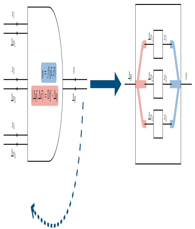
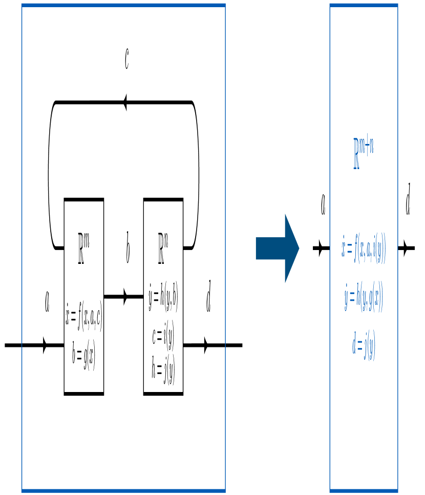
The process of training a deep neural network (DNN) can be described as follows: an input-output pair is given (this is a training datum); the DNN uses its current parameters to push the given input from the start to the end of the network; the DNN compares the final result of this forward pass against the given output, and propagates the error backward through the network, updating its parameters as it goes; the whole process is repeated many times. DNNs are commonly drawn as networks of artificial neurons; it is through the wires connecting the “neurons” that information is passed, and information is passed in both directions. Because of this, our first slight modification to these pictures is to double each of the wires, resulting in two unidirectional paths instead of one bidirectional path, as shown in the left-hand side of Figure 1. Now the wires running from left to right (labelled $x_{i}$ , $y_{i}$ , etc.) correspond to the forward pass, and the wires running from right to left (labelled $\Delta x_{i}$ , $\Delta y_{i}$ , etc.) correspond to the backward pass.

The most important mental move required to understand the mathematical analogy we are building is as follows. Imagine taking a single “neuron”, along with its input and output wires, and “unfolding” it into a different shaped diagram, as shown in Figure 1. Doing so results in a trivial example of something called a interaction diagram, and, as we will discuss, these objects give a very useful way of describing interacting dynamical systems (IDSs).

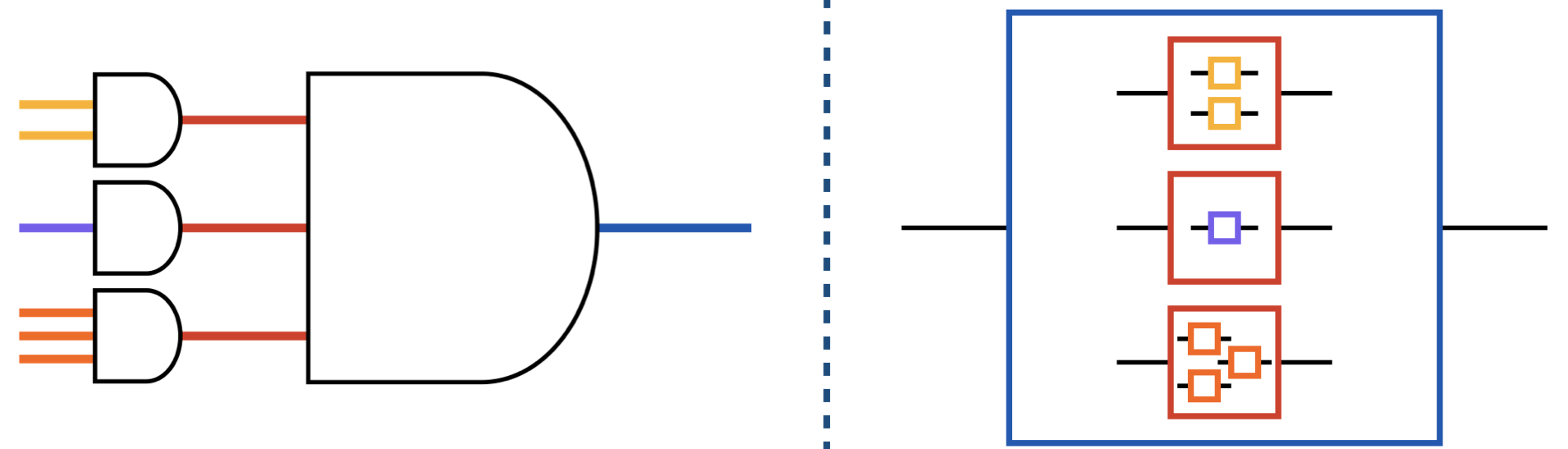
Refer to caption — Figure 1: By grabbing hold of the wire labelled $\Delta y$ and dragging it along the dotted arrow, we can “unfold” our artificial neuron (shown left) into an interaction diagram (shown right), so that the inputs and output to the artificial neuron turn into interior boxes and exterior box respectively.

Generalising the above procedure to multiple “neurons”, as in Figure 2, we see how left-to-right composition turns into so-called operadic composition, given by nesting interaction diagrams inside other interaction diagrams.

Before going any further though, let us take a moment to pause and gain some intuition on how to read interaction diagrams. We can think of each box as a person holding an office—it is important that we really mean both a person and the office that they hold; the person can make decisions, and the office has attendant capacities that allow the person to abstract the information they receive from the world (not just from subordinates, but from their superiors as well). That is, the person is given lower-level data and turns it into higher-level data. We refer to the person as the abstractor and the function of their office (i.e. how it interacts with the rest of the world) as the abstraction.

Now we can understand the interaction diagram for DNNs in Figure 1 as follows. There are three smaller abstractors (which we will call “workers”), whose offices are in the purview of a higher-level abstractor (which we will refer to as M, for “manager”), drawn as an encompassing box. So M receives information from the outside (the “input”, which we can think of as feedback, as in “good job” or “make this correction”) and is tasked with calling out some sort of processed information (the “output”) back to the outside world. The way that M does this is by updating its methodology (namely, how much it listens to, or trusts, each of its subordinate workers; the associated weights and biases), as well as passing along to each worker W the part of the input that corresponds to W’s office (that is, the feedback specific to that worker). This recurses inwards: each worker does whatever it is that they have been trained to do, sends feedback to and then listens to subordinates, and shouts out the results to its superiors. In proportion to how loudly each worker shouts, and according to M’s current weights and biases, M receives the three outputs and combines them to give the final output, which it shouts out. Note that M is also shouting things out here—this whole system can recurse outwards as well, with M being subordinate to some other, higher-level managers. In DNNs, the levels of this hierarchy are called layers.

Of course, this scenario where workers are competing in a shouting match to get their manager to listen to them is not really the description of an ideal working environment. Most notably, the workers in DNNs never talk to each other or collaborate. And yet this is how almost all neural networks work today; the only thing an artificial neuron can do is add up incoming signals according to weights and biases. Note that even weight tying, as in convolutional or recurrent neural networks, does not address the point we’re making here. Certain loss functions—as seen in physics-inspired neural networks, for example—do make a small amount of headway, but the breadth of what is possible here does not seem to be known in the machine learning community. To remedy this, we will explain in the next section an idea that is well-known in the control theory community.

Just to be clear though, this problem is not simply due to the fact that we are considering one single artificial neuron, or that there is no feedback in the typical diagram, as one might imagine is remedied by recurrent neural nets. Again, having loops in a typical DNN diagram does not type check with the remedy we’re proposing, because nerve cells are playing the role of wires in these typical diagrams. The unfolded diagrams give a pictorial representation that clarifies how to see the nerve cells (which were the wires and are now the boxes) as interacting. Even in the case of multiple “neurons" (cf. Figure 3), although there are more levels of nesting, there is still no “peer-to-peer communication”. Thus we are ready to pose the question, “what if we allowed our DNNs to have internal wiring?” (cf. Figure 4).

2

Let us now take some time to discuss interaction diagrams—a generalization of something called wiring diagrams or block diagrams, commonly found in control theory—and how they describe interacting dynamical systems. Here we will see that, although such diagrams gain a great deal of generality by having non-trivial wirings, they have no notion of adaptivity, as found in DNNs.

Consider a computer processor. It consists of many (many) small parts, and these small parts are made up of even smaller parts: the circuit board has adders, which are made up of logic gates, which are made from transistors, and so on. Using the language from before, we can say that the adder is an abstractor of the logic gates, and the logic gates themselves are abstractors of the transistors. Some abstractions are more useful than others, so people have spent a great deal of effort in finding the right abstractions, such as NOT, AND, OR, etc. At each level of this hierarchy, the parts interact with each other, resulting in the processes which combine to give the functionality of the processor as a whole. But then the processor itself forms a smaller part of a larger system, such as a computer, or a mobile phone, and these in turn might combine to form networks with their own emergent behaviour. This is an example of operadic composition of systems, which is the formal way of specifying how simpler abstractions can be combined to form higher level ones.

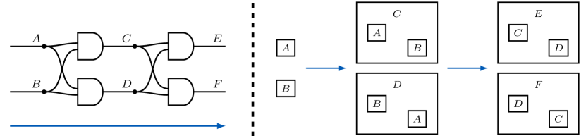
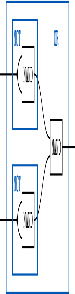
We can draw these systems and subsystems using interaction diagrams. For example, Figure 5 shows how we can construct the logical OR gate using NAND gates. But these diagrams are not simply convenient pictorial representation of the dynamical systems which they describe; instead, using category theory, we can regard these diagrams as formal mathematical objects, whose combinatorics is the subject of mathematical statements and proofs. Figure 6 gives an example of this, showing that we can embed a certain sort of mathematical objects (here, systems of ODEs) into these diagrams, and get another such object (a combined ODE) as a result.

In this diagrammatic approach to studying interacting dynamical systems, the base-level systems are dynamic and changing, but the formalism seems to insist that their interaction pattern is itself fixed in time. Indeed, if we imagine the actual electronic circuit described by Figure 5, for example, then the connections would be permanently soldered, and the way in which the subsystems interact would never change. Of course, from the birth of modern electronics up until now, fixed interaction patterns have proved very useful—we’re not denying that! But in real life, the wirings between systems can often change: FPGAs provide one example, but so do more general scenarios, such as the way that mobile phones move in and out of range of network coverage, causing reconnection to different cell towers. We can even consider the problem of studying human society as a dynamical system, and here the connections are constantly changing: two people who might be “wired together” (e.g. talking via video call) at one point in time will then be “un-wired” (e.g. ending the call) at a later point in time. In the language of interaction diagrams, allowing such continuous changes in interaction patterns is called dynamic rewiring, and it’s becoming increasingly important to have a mathematical account of.

One of our earlier claims was that DNNs already have the capacity for such dynamic rewiring. Indeed, this is inherent in the way that these systems learn: the values of weights and biases change after every batch of training data. So by unfolding the usual neuron picture into the interaction diagram picture (see Figure 1), and thinking of the nerve cells as the interior boxes (note that these two changes are enough to repair the usual analogy), we have allowed our DNNs to have peer-to-peer messaging, but have perhaps lost the possibility for changing interaction patterns.

The question then, is the natural one: “can we have the best of both worlds, allowing our systems to have (a) non-trivial peer-to-peer wiring, that (b) can change and adapt through time?”

3

Using category theory (or, more specifically, the formalism of polynomial functors), one can give a positive answer to the above question. The two generalisations that we have described actually give one single structure: an interacting dynamical system with dynamic rewiring and a deep neural network with peer-to-peer messaging are simply two different descriptions of the same mathematical object, which we call deeply interactive learning systems (DILSs). Passing between these two viewpoints allows us to better understand the analogy between them.

With DILSs, there is no longer the usual discrete partition of the learner into “learning phase”, “testing phase”, “implementation phase”—instead, the system is continuously online, embedded in an actual world, as is the case in control theory. The usual notion of trainer is replaced simply by prediction error: how well the high-level abstractions actually offer affordances to the system. From the DNN point of view, “the current collection of weights and biases” is generalised to “the current interaction pattern between components”. Furthermore, these interaction patterns are much more collaborative and cooperative than the simple “shouting match” described by weights and biases. It also helps us to understand the relation between data as it flows through the DNN, as well as abstraction itself: the lefthand layer corresponds to low-level data (think “pixels”); the right-hand layer corresponds to high-level data (think “cat”); processing data corresponds to creating higher-level abstractions (think “pixels become curves and features, which become… ears and whiskers, which become a cat”). This corresponds to the movement from interior to exterior boxes of Figure 4, whereas the movement from left to right wires correspond more to going from sensory input to motor output.

	Hierarchy direction	Peer-to-peer messaging?	Changeable interaction pattern?
DNN	left $\to$ right	✗	✓
IDS	inside $\to$ outside	✓	✗
DILS	either/both of the above	✓	✓

Interacting dynamical systems with fixed wiring have been extraordinary useful over the past-half century, but they are inherently static. The power of deep neural networks explicitly relies on dynamic rewiring, but they neglect the possibility of peer-to-peer messaging. Category theory allows us to combine the strengths of these two architectures into one more general framework (whose applications are as yet unexplored), whilst also correcting the structural flaw in usual analogy between deep neural networks and brain anatomy.

Reading list

1.

GSH Cruttwell, B Gavranović, N Ghani, P Wilson, F Zanasi. “Categorical Foundations of Gradient-Based Learning.” (2021) arXiv: 2103.01931.
2.

B Fong, D Spivak, R Tuyéras. “Backprop as Functor: A compositional perspective on supervised learning.” 2019 34th Annual ACM/IEEE Symposium on Logic in Computer Science (LICS) 1 (2019), 1–13. DOI: 10.1109/LICS.2019.8785665.
3.

B Fong, D Spivak. An Invitation to Applied Category Theory: Seven Sketches in Compositionality. Cambridge University Press, 2019. DOI: 10.1017/9781108668804. (Freely available online as arXiv:1803.05316).
4.

T Mitchell et al. “Never-ending learning.” Communications of the ACM 61 (2018), 103–115. DOI: 10.1145/3191513.
5.

P Selinger. “A Survey of Graphical Languages for Monoidal Categories”, in New Structures for Physics. Springer, 2010. Lecture Notes in Physics 813. DOI: 10.1007/978-3-642-12821-9_4.
6.

D Vagner, D Spivak, E Lerman. “Algebras of open dynamical systems on the operad of wiring diagrams.” Theory and Applications of Categories 30 (2015), 1793–1822.