Acoustic Cloak Design via Machine Learning

Abstract

Acoustic metamaterials are engineered microstructures with special mechanical and acoustic properties enabling exotic effects such as wave steering, focusing and cloaking. The design of acoustic cloaks using scattering cancellation has traditionally involved the optimization of metamaterial structure based on direct computer simulations of the total scattering cross section (TSCS) for a large number of configurations. Here, we work with sets of cylindrical objects confined in a region of space and use machine learning methods to streamline the design of 2D configurations of scatterers with minimal TSCS demonstrating cloaking effect at discrete sets of wavenumbers. After establishing that artificial neural networks are capable of learning the TSCS based on the location of cylinders, we develop an inverse design algorithm, combining variational autoencoders and the Gaussian process, for predicting optimal arrangements of scatterers given the TSCS. We show results for up to eight cylinders and discuss the efficiency and other advantages of the machine learning approach.

Research

Introduction

Acoustic metamaterials are engineered microstructures with special mechanical and acoustic properties such as negative effective mass density, bulk modulus, and refractive index [1, 2, 3, 4]. The unique arrangement of components in metamaterials gives rise to exotic interactions with acoustic waves at large wavelengths. This has many applications such as wave steering [5], cloaking [6, 7], and focusing [8, 3, 9]. The traditional method of designing acoustic cloaking devices involves direct computer simulation [10], topology optimization [11], stochastic optimization [12, 13], and gradient based optimization[7, 14] of the acoustic response based on the structure. The direct forward methods require the iterative process of trial and error, leading to sub-optimal performance of metadevices. The computational costs for non-convex optimization problem in a high-dimensional space including stochastic optimization, adjoint based design and gradient based optimization are high and present an immense computational challenge [15, 16]. While these approaches have shown improvement in efficiency and performance over the years, they are still ineffective in the inverse design of broadband metamaterials and metadevices, specifically in predicting the structure parameters given the acoustic response at different values of frequencies or incident angles.

The last decade has witnessed a surge of scientific publications in which deep learning, reinforcement learning and generative modelling were applied in different areas of science and engineering [17, 18, 19, 20]. Recent advances in the field of machine learning have enabled a new, data driven, approach with a great promise to solve problems such as the inverse design in acoustic metamaterials [21, 22, 23, 24, 25]. Early machine learning applications in acoustic forward design date back to the late 90s when Jenison first used spherical basis function of fully-connected neural networks (FC) for approximating the acoustic scattering of a rigid scatterer [26, 27]. Hesham and El-Gamal [28, 29] later solved an integral equation of acoustic scattering using wavelet basis and FC.

More recent works have proven that machine learning is much more efficient than numerical methods in both forward and inverse design of metamaterials. For example, Gnecco et al. [30] employed principal component analysis (PCA) to gradient fields in spectral design of acoustic metamaterials, solving constrained nonlinear optimization problems. Fan et al.[31] formulated acoustic scattering by a single scatterer as a 2D image-to-image regression problem using convolutional neural networks (CNN). In their model, the inputs were the images of convex prism objects, including circular and ellipsoidal cylinders, and square bars; the outputs were the loudness fields computed using the Triton system that employs the fast adaptive rectangular decomposition pseudo-spectral wave solver. Fan et al.[32] developed a CNN to predict the object geometry from acoustic scattering given the images of total acoustic field as inputs to CNN. Meng et al. [33] investigated the inverse acoustic scattering problem that reconstructs the obstacle shape with far-field information using fully connected neural network (FC). Shah et al.[22] employed deep reinforcement learning algorithms to design acoustic cloaks by adjusting positions and radii of cylindrical structures; these reinforcement learning models are capable of predicting better results than the-state-of-the-art gradient based optimization algorithms. Wu et al. [23] proposed machine learning framework for the design of one-dimensional periodic and non-periodic acoustic metamaterials using deep learning and reinforcement learning algorithms. Alternative machine learning methods such as powerful deep generative models, including generative adversarial networks [34, 21], autoencoders [25, 24], and variational autoencoders (VAE) [25, 35, 36] are also able to produce synthetic structures after being trained on real examples.

Most of the studies mentioned above succeed with predicting the acoustic response based on the structures. However, the challenge of finding a streamlined approach in designing structures with a desired acoustic response is still in its infancy. In this study, we continue tackling this inverse design problem by proposing a promising new method. First we show that FC and convolutional neural networks can be trained to predict the acoustic response based on the locations of cylindrical structures (forward design). We then implement a VAE to convert the structures into a latent space and train it together with a regressor that is capable of yielding the total scattering cross section (TCSC) given the latent variables. By performing Bayesian optimization using the Gaussian process (GP) in the continuous latent space, we demonstrate that one can quickly find new configurations with minimal TSCS. Our method, which is straightforward to implement and computationally cheap to operate after training, has great implications for metamaterials design with on-demand properties.

Method

Multiple Scattering Theory

In order to analyze how sound is scattered in acoustic media, we use the multiple scattering theory [37]. We consider multiple scattering in the context of the acoustic time harmonic wave equation in two dimensions. The total acoustic pressure field $p({\bf x})$, ${\bf x}\in{\cal R}^{2}$ is defined as the sum of incident $p_{inc}$ and scattered $p_{sc}$ pressure fields:

$$p=p_{inc}+p_{sc},$$ (1)

which satisfies the Helmholtz equation:

$$\nabla^{2}p+k^{2}p=0,$$ (2)

where $k=\omega/c$ is the wavenumber, $c$ is the acoustic speed, and $\omega$ is the frequency. As a measure of the scattering, we use the TSCS which is denoted by $\sigma$. We use the optical theorem [38] to relate the TSCS to the scattering amplitude in the forward direction, i.e. the direction of propagation of the incident plane wave, here assumed to be the positive $x-$direction [7]:

$$\sigma=-2\textrm{Re}f(0),$$ (3)

where the far-field amplitude form function, $f=f(\theta,\,{\bf r}_{1},\,{\bf r}_{2},\ldots,{\bf r}_{M})$, $\theta=\arg({\bf x})$, is the angular part of the scattered pressure $p_{sc}$ in the far-field in terms of position vector, and ${\bf r}_{1},\,{\bf r}_{2},\ldots,{\bf r}_{M}$ denote the positions of each scatterer. Here, $f(0)=f(\theta=0)$. A more detailed description of multiple scattering problem formulation can be found in Refs. [37, 22, 7, 39]. Our goal in this study is to find an efficient way to obtain scatterer locations that minimize $\sigma$ at certain wavenumbers (inverse design), and hence, pave the way for the creation of acoustic cloaks.

Data Generation

Datasets for TSCS of different configurations of rigid cylinders are generated using the multiple scattering solver [7, 39] implemented in MATLAB. For a given configuration of scatterers, $\sigma$ is evaluated at discrete values of the normalized wavenumber $ka$. We first randomly position $M$ uniform cylinders of radius $a$ inside an artificial circular region of radius $R=6a$ as depicted in Fig. 1 (a) and (b). We keep the minimum distance between the cylinder centers as $|{\bf r}_{i}-{\bf r}_{j}|=2a+\delta$ where $\delta=0.1a$ [7]. The images contain $28\times 28$ binary pixels; taking the value $1$ for the area of rigid cylinders, denoted by the color white, and $0$ for the exterior fluid, denoted by the color black. Then $\sigma(k_{i}a)$ is evaluated at 11 discrete values of wavenumber $ka\in[0.35,0.45]$ and $ka\in[1.35,1.45]$ using Eq. (3). Fig. 1(a)-(d) show sample configurations for $M=2$ and $M=6$ along with their corresponding $\sigma$’s as functions of the wavenumber. Figs. 1(e)-(h) show histograms of $\sigma$ over the entire data at select $ka$’s within two different intervals that we have considered in this study.

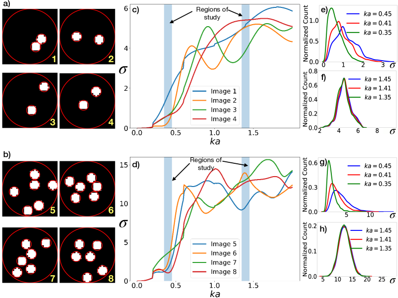
Figure 1: Random configurations generated in binary images, (a) and (b), and their corresponding total scattering cross section $\sigma$. (c) and (d) show the TSCS values as a function of $ka$ for $4$ different $28\times 28$ images of $M=2$ and $M=6$ from panel (a) and (b). The white dots represent the rigid cylindrical scatterers of radii $a$. The scatterers in (a) and (b) are confined to an artificial circle of radius $R=6a$ with minimum distance between the cylinder centers $|{\bf r}_{i}-{\bf r}_{j}|=2a+\delta$, where $\delta=0.1a$. (e)-(h) show the normalized count of the total scattering cross section used for training. The three sample wavenumbers shown in each plot belong to two different regions, $ka\in[0.35,0.45]$ and $ka\in[1.35,1.45]$. In the smaller $ka$ region, distributions gradually shift to the right for larger wavenumbers while they mostly overlap in the larger $ka$ region.

Forward Design

We employ both FC and CNN in our forward design. The goal is for the feed-forward artificial neural network to predict the TSCS (learn the nonlinear function of $ka$) given the scatterer positions. We provide the networks with binary images of scatterer configuration as input for the training. The dataset for each $M$ is split into $54,000$ ($90$%) samples for training and $6,000$ ($10$%) samples for unbiased validation during training. Experimenting with different image sizes ranging from a few hundreds to thousands of pixels, we find that the image resolution does not affect the outcome significantly, and therefore, we have chosen $28\times 28$ images for training to avoid unnecessary computational costs.

For the FC, we design a 3-hidden-layer network with 100 nodes each. In that case, the $28\times 28$ input image is flattened into a one-dimensional vector of length $784$ before feeding it into the fully connected layers. Since all of the pixel values are used for training, the neural network is highly susceptible to overfitting when training with $M\geq 6$. Hence, a dropout layer with rate of $0.2$ is added after the third hidden layer.

The CNN is our primary focus because of its ability to leverage spatial correlations in an image, which would otherwise be lost during image flattening step of a FC. Fig. 2 illustrates an example of our CNN architecture. In contrast to the FC, the CNN passes an image through a series of convolution and pooling layers for feature extraction. Specifically, in the first convolution layer a $3\times 3$ kernel matrix slides across the image, convolving with portions of it, and passing the information to later layers. In the first pooling layer, only maximum pixel values in $2\times 2$ blocks of feature maps are selected, reducing the resolution and removing redundant information in order to mitigate overfitting. Finally, the output of the last pooling layer is flattened and fed into one layer of fully connected nodes before decision making in the output layer. Overall, the network learns to make prediction by optimizing its weights and biases. These parameters are continually adjusted during the training process until the mean squared error between its output and the exact TSCS saturates (see Appendix).

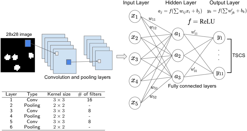
Figure 2: A diagram of forward design used for TSCS regression. The input image is first passed through a series of convolutional and pooling layers in which the kernel, depicted by the small blue square, sweeps through the input image to extract features and reduce the dimensions. The table below shows the details of each layer. Next, the resulting output is flattened and fed into a fully connected neural network. The input layer $x_{i}$ no longer represents the pixel values from the original image but rather abstract image attributes. The activation function of perceptrons is $f=$ ReLU (rectified linear unit). The output layer comprising of 11 perceptrons for the TSCS values, which are compared to the true values during training by the loss function of mean squared error.

Inverse Design

VAE is a probabilistic generative model that uses Bayesian inference combined with a neural network to approximate the distribution of data [40]. The model learns from examples and compresses the original data into a low dimensional and continuous representation called latent space, characterized by a latent vector $z=(z_{1},z_{2},\dots)$. The number of latent variables generally determines the amount of information or relevant features that can be encoded into the latent space. We apply VAE to our datasets of images of different cylindrical configurations. After training the model, sampling from the latent space allows us to generate new, unseen images. However, in addition to the plain VAE, which simply approximates the input image data, we condition the VAE with TSCS, so that the latent space does not only reflect the positional characteristics of the scatterers but also their corresponding TSCS. We perform this conditioning procedure within two different methods: supervised VAE (SVAE) [41] and conditional VAE (CVAE) [42]. We then examine the statistics of the latent variables from the two modified VAE models and search for new configurations with minimum TSCS. Figure 3 shows the details of the VAEs architecture and layers used to train the models in our study.

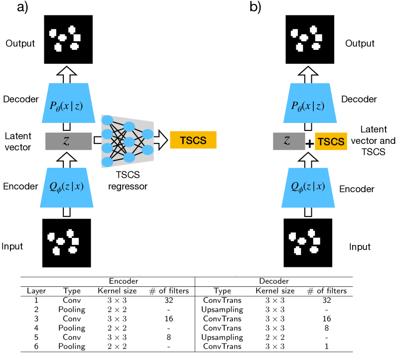
Figure 3: The two variational autoencoder (VAE) architectures used for inverse design: a) supervised VAE and b) conditional VAE. Starting from an image of scatterers, the encoder transforms the image into a lower-dimensional, continuous representation vector $z$. In a) this latent vector is fed into a TSCS neural network regressor made of 3 layers, whereas in b) the TSCS is directly embedded into the latent by concatenating the two vectors. The decoder converts the latent vector back into the original input image. By incorporating the TSCS into VAEs, we condition the networks to organize the latent variables in accordance with the physical information offered by the TSCS. We then use this latent space to perform optimization and search for the configuration with the lowest TSCS. The table at the bottom shows the layers used in the encoder and the decoder. We used ReLU as the activation for the middle layers and sigmoid for the output layer. (Conv: convolution; ConvTrans: convolution transpose)

The goal of VAEs is to estimate the true distribution of input images $P_{\theta}(x)$ using a neural network:

$$P_{\theta}(x)=\int P_{\theta}(x|z)P(z)dz=\int P_{\theta}(z|x)P(x)dz,$$ (4)

where $x$ is the input data, $z$ is the latent variable drawn from a predefined distribution $P(z)$, and $\theta$ are the model parameters. The problem with maximizing the likelihood of obtaining $z$ given $x$ is that the above integral is intractable due to the large number of parameters $\theta$ produced by the neural network. Instead, VAEs approximate $P_{\theta}(z|x)$ with an encoder $Q_{\phi}(z|x)$, which is often chosen to be a multivariate Gaussian distribution:

$$Q_{\phi}(z|x)=\mathcal{N}(z;\mu(x),diag(s(x)))$$ (5)

The above equation implies that each latent variable, after being trained on data, should follow a normal distribution with mean $\mu(x)$ and standard deviation $s(x)$, independently of one another. The inference model $Q_{\phi}$ takes in the input image and generates the latent variable $z$ while the decoder $P_{\theta}(x|z)$ reconstruct the original input based on $z$, as depicted in Fig. 3. The difference between the two conditional distributions is determined by the Kullback-Leibler (KL) divergence:

$$D_{KL}(Q_{\phi}(z|x)|P_{\theta}(z|x))=\mathbb{E}_{z\sim Q}[\log Q_{\phi}(z|x)-\log P_{\theta}(z|x)].$$ (6)

Using Bayes theorem, $P_{\theta}(z|x)=P_{\theta}(x|z)P(z)/P_{\theta}(x)$, we replace $P_{\theta}(z|x)$ in Eq. (6) to obtain

$$\log P_{\theta}(x)-D_{KL}(Q_{\phi}(z|x)|P_{\theta}(z|x))=\mathbb{E}_{z\sim Q}[\log P_{\theta}(x|z)]-D_{KL}(Q_{\phi}(z|x)|P(z))$$ (7)

Maximizing the left side of Eq. (7), also known as finding the variational lower bound or evidence lower bound, means optimizing the model parameters $\phi$ and $\theta$ of the neural network via backpropagation. As the model is trained, the encoder $Q_{\phi}(z|x)$ and the decoder $P_{\theta}(x|z)$ will become better at encoding the attributes $z$ given data $x$ and reconstructing the data $x$ given the latent vector $z$. In other words, we want to minimize the KL divergence on the left hand side of Eq. (7), which translates to maximizing the term $\mathbb{E}_{z\sim Q}[\log P_{\theta}(x|z)]$, or minimizing the reconstruction loss ($\mathcal{L}_{R}$), and minimizing the KL divergence loss ($\mathcal{L}_{KL}$) in the right hand side of Eq. (7). The former is simply the mean squared error between the input and the reconstructed image, and the latter is accomplished by adjusting the network parameters in the encoder ($\phi$) during training to match the network distribution for $z$ given the images and the desired normal distribution.

This training of the VAE requires reparameterization of the encoded sample $z$ drawn from the predefined normal distribution as:

$$z=\mu+\epsilon s$$ (8)

where $\epsilon\sim\mathcal{N}(0,1)$ [40]. This ensures backpropagation gradients passing through all layers.

In the next step, in order to implement a SVAE and bring in the physical property of interest, we add another neural network regression model that takes in the encoded latent variables $z$ as input and predicts the TSCS. The TSCS regression model loss ($\mathcal{L}_{TSCS}$) is minimized simultaneously along with KL and reconstruction loss during training:

$$\mathcal{L}_{SVAE}=\mathcal{L}_{R}+\mathcal{L}_{KL}+\mathcal{L}_{TSCS}$$ (9)

In addition, we also experimented with CVAE by directly embedding the TSCS into the input data used for training. In that case, Eq. (7) becomes:

$$\log P_{\theta}(x|c)-D_{KL}(Q_{\phi}(z|x,c)|P_{\theta}(z|x,c))$$ (10)

$$\quad=\mathbb{E}_{z\sim Q}[\log P_{\theta}(x|z,c)]-D_{KL}(Q_{\phi}(z|x,c)|P_{\theta}(z|c)),$$

where $c$ is the conditional vector, in our case the TSCS corresponding to each input image, that we concatenate with $z$. The TSCS regressor, which was used as the objective function to minimize in the SVAE, is substituted in this case by the combination of the decoder part of the VAE and the trained CNN model from forward design, which takes as input the images produced by the decoder.

After acquiring a continuous representation of the data through the latent variable, we perform global optimization in the latent space using a Gaussian process [43]. The Gaussian process is extremely robust in predicting any smooth and nonlinear function based on data. First, we obtain a surrogate function by training a GP model to approximate the TSCS regressor given the latent variables as input. Then, we minimize this surrogate function through Bayesian optimization to search for $z$’s that correspond to configurations with the lowest TSCS. In the next step, we decode those $z$’s back to images using the trained decoder from our VAE models. Finally, the suggested positions of the cylinders in the decoded image are converted back into physical coordinates to compute the TSCS with our analytical solution for comparison.

Optimizing the probabilistic GP model, as opposed to working with the trained fully connected neural network regressor, is the key step here that allows us to perform the inverse design. Moreover, it provides a smoother search space and the function is cheaper to evaluate too. The advantage of including the regressor in the SVAE, or concatenating $z$ with TSCS in the CVAE, is that we are conditioning the latent variables to reflect TSCS, and hence, forcing the neural network model to encode the physics of the problem as opposed to simply the whereabouts of the scatterers.

Results

We used Tensorflow [44] python libraries with Keras application programming interface, the open source machine learning framework, to build, train, and test our models. We first discuss the performance and limitations of FC and CNN in forward design. Next, we report the outcome of VAEs in inverse design followed by the optimization results of the TSCS with respect to the latent variable.

Convolutional Neural Networks and the Forward Design

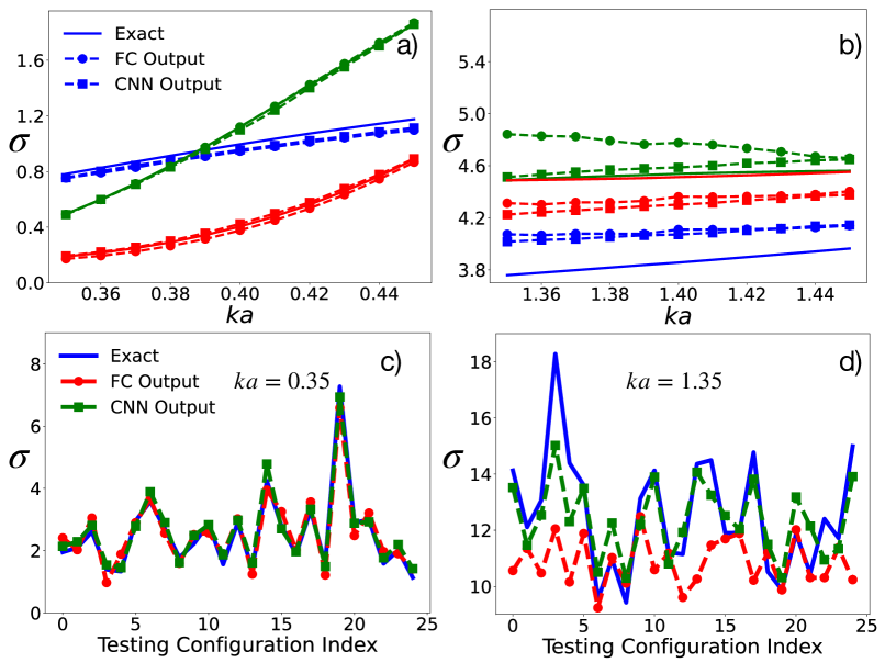
Figure 4: The exact total scattering cross section (TSCS) plotted along with deep learning model predictions. The top row shows the TSCS for three samples with $M=2$, evaluated across $11$ wavenumbers in two regions: (a) $k_{i}a\in[0.35,0.45]$ and (b) $k_{i}a\in[1.35,1.45]$, where $i=\overline{1,11}$. The bottom row shows the TSCS of $25$ samples with $M=6$, evaluated at single wavenumbers (c) $ka=0.35$ and (d) $ka=1.35$. Note that these are separate models trained in two different regions of wavenumbers, and in general the lower $ka$ region tend to produce more accurate approximation.

Figure 4 shows the training results with the top row plotting the TSCS when $M=2$ as a function of the wavenumber for three random sample images, and the bottom row displaying the output when $M=6$ at two different wavenumbers across many samples. We experimented with both FC and CNN in forward design. Fig. 4(a) and 4(b) show results for each of the two wavenumber regions highlighted in Fig. 1(c). Each color in those panels represents results for a different binary image of the scatterer configurations, and different lines distinguish the exact results from those obtained through the FC or the CNN. Note that the models are trained separately in the two regions of the wavenumber: $k_{i}a\in[0.35,045]$ and $k_{i}a\in[1.35,1.45]$.

As can be seen, the network performs worse in the larger wavenumber region [e.g., in Fig. 4(b)]. The decrease in the prediction accuracy can be explained by the relatively small variation in TSCS, both from a configuration to another and also across $ka$ in that region, making it harder for the network that now has to learn subtle differences. This fact can be inferred from the distributions shown in Figs. 1(e)-(h). In the large wavenumber region [Figs. 1(f) and 1(h)], the distributions of TSCS in $ka$ are narrower, and also more similar at different $ka$, than in the smaller wavenumber region [Figs. 1(e) and 1(g)]. We also observe that for these small $M$, FC and CNN have more or less the same level of performance.

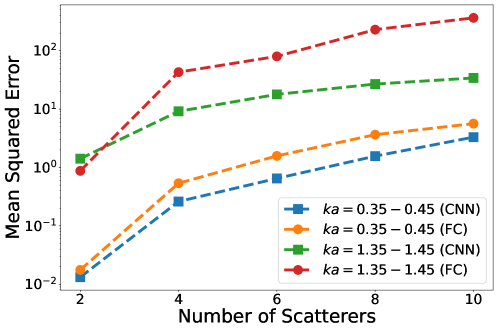
Figure 5: The average mean squared error between exact and predicted TSCS, computed over the testing set of $6,000$ samples in two regions of wavenumber. Note that the error is greater when training with larger wavenumber and with greater numbers of cylinders. This figure also clearly shows that the CNN generally outperforms the FC neural network.

Similar trends are seen in Figs. 4(c) and 4(d) across 25 different input configurations with $M=6$ and at a select $ka$ in each of the wavenumber regions. These plots make it clear that as $M$ increases, the CNN generally outperforms FC, as we expected.

In general, the training accuracy decreases as the number of cylinders increases. This can be seen in Fig. 5, where the average mean squared error, $\sum_{i}^{N}{(y_{i}^{predicted}-y_{i}^{exact})^{2}}/N$, where $N=6,000$ is the total number of testing samples, is shown. As expected, the difference in error between CNN and FC is slightly greater in the larger $ka$ region. In training the neural network, we have noticed that the network is prone to overfitting when $M\geq 6$, so in those cases we have added a dropout layer, which effectively reduced the numbers of neurons during training. We also observe that CNNs were more resistant to overfitting and generally outperformed FCs.

Variational Autoencoders and the Inverse Design

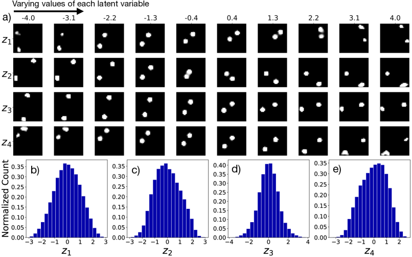
Figure 6: Change of scatterer configurations upon changing each of the latent variables $z_{i}$ of a trained VAE. We have used the trained decoder to generate new images for the $M=2$ case by sampling from the $z_{i}$ distributions. The first row of panel (a) shows what happens to the two cylinders when $z_{1}$ increases while the other three latent variables remain unchanged. The next three rows corresponds to varying $z_{2},z_{3}$ and $z_{4}$. The distance between the two cylinders changes as we vary each latent variable, along with the angle of the line connecting them. Panels (b)-(e) show the histograms of each latent variable, which follow the normal distribution as expected.

While it is difficult to interpret what exactly each latent variable represents after training a VAE, Fig. 6(a) attempts to illustrate what attributes of the image the network has learned for the case of $M=2$, in which the latent space has only $4$ elements. For example, the first row shows what happens to the location of the two cylinders as the value of $z_{1}$ changes while other latent values remain fixed. The second row demonstrates the change of locations as only $z_{2}$ varies, and so on. Even though varying any of the latent values results in a slight difference in location of the scatterers, we find that, for example, $z_{2}$ values are mostly associated with the distance between the two cylinders. Increasing negative $z_{2}$ values decreases this distance. Then, upon the change of sign of $z_{2}$, the orientation of two cylinders changes suddenly before the distance between them increasing slightly again with further increasing $z_{2}$. $z_{3}$ appears to be responsible for a simultaneous change of distance between the cylinders and their rotation while increasing $z_{4}$ seems to increase that distance and uniformly translate the cylinders at the same time.

Figure 6(b)-(e) are the distributions of the encoded latent variables of $6,000$ testing samples. Each latent variable follows roughly a normal distribution with mean and variance close to zero and one as expected, since the values of $z$ were sampled from a multivariate normal distribution during training. Whereas only $4$ latent variables were needed to achieve a high training accuracy for $M=2$, the length of the latent vector must be at least $40$ to reach a reasonable accuracy for $M\geq 8$. In general, the more latent variables, the better the accuracy. However, optimization with a large number of variables could be time consuming.

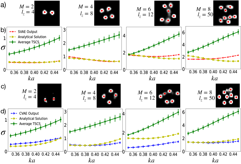
Figure 7: Generated samples from variational autoencoder models and their TSCS for $M=2,4,6$ and $8$. (a) and (c) are binary images produced by optimizing the latent space of each respected configuration of $M$ scatterers using SVAE and CVAE. The number of latent variables used in training the models and optimization is listed on the left side of each image. The red dots, which are obtained by thresholding the decoded images and finding the center of mass among the pixel values, indicate the positions of the cylinders. (b) shows the SVAE output, which is the same as the TSCS regressor output. (d) shows the CVAE output computed by the trained CNN model from forward desired. The average TSCS for each wavenumber $ka$ of $30$ randomly selected training examples and their standard error is also plotted for comparison. While the semi-analytical solution does not match the regressor output completely, the optimized configurations clearly have much lower TSCS compared to the average TSCS.

After obtaining the continuous representation of the images through the latent space, we use a Gaussian process to search for optimized configurations within the latent space. The optimal set of latent variables must reflect both a high probability of being drawn from the normal distribution and a low TSCS.

In designing the architecture for SVAE, we find that the TSCS regressor, when trained to predict the TSCS of more than one wavenumber, surprisingly performed better than when trained to predict only the TSCS of a single wavenumber. This is a promising sign because it suggests that expanding our region of interest in $ka$ [see Fig. 1(c)] in future studies can potentially improve the performance of our approach.

Figures 7(a) and 7(b) show the optimization results for $4$ different $M$’s using the SVAE. The Gaussian process generated many samples with low TSCS, but here we showcase only one representative sample. The numbers of latent variables used for the optimization are $l_{z}=4,8,12,50$ for $M=2,4,6,8$, respectively. The optimal latent values are decoded into images shown in Fig. 7(a) by the SVAE’s trained decoder. As shown in Fig. 7(b), while the average TSCS over all the training images (green curve) generally increases with $ka$, the SVAE is able to produce new configurations with constant or slightly decreasing TSCS, as indicated by the red curve.

To ensure the SVAE did not simply memorize the training data, we searched for similar configurations from the $60,000$ samples used to train our models. We compared the generated images and observed that the majority of generated configurations, except for the case of $M=2$, were indeed distinct variations of the existing training data. We note that a small change in position of only one cylinder could result in a drastic change in the TSCS output.

The locations of the cylinders in generated images, marked by the red dots, are estimated by thresholding each image within an appropriate pixel range and calculating the center of mass of the pixel values. The centroid positions are then used to compute the analytical solution of the TSCS. As can be seen in Fig. 7(b), the SVAE output is in good agreement with the semi-analytical solution.

Fig. 7(c) and (d) show optimization results for CVAE. To prompt the decoder to generate images with TSCS close to zero, we input $11$ zeros as the conditional vector $c$ of Eq. (10). However, we find that the CVAE does not independently produce images with low TSCS this way; the additional minimization step through a surrogate model is required. Therefore, similarly to the case of SVAE, we use GP to search for possible latent values (excluding the conditional vector) with the lowest TSCS. The only difference is that the TSCS regressor in SVAE is replaced by the combination of the decoder and the trained CNN from forward design. As can be seen in Fig. 7(c) and (d), the results are encouraging and comparable to those obtained through the SVAE.

We observe that generally, optimizing the objective function with larger numbers of latent variables can result in clearer and more realistic samples but also takes a longer time. This can be inferred from sample images in Fig. 7(a) and (c), where those corresponding to $M=8$ seem to be sharper than the images for $M=6$ despite having more cylinders. This is at least partly due to the fact that the VAE models for $M=8$ were trained with greater number of latent variables ($l_{z}=50$) compared to $l_{z}=12$ for $M=6$. For $l_{z}\leq 50$, the objective function converges to a minimum value within a few minutes using the Gaussian process optimization.

In analyzing the resolution of the generated images, we noticed that some of the cylinders, represented by the white regions, are blurry or have lower pixel values, suggesting that these cylinders might not be as important as others. This is interesting since it shows that the machines might be able to predict different size cylinders for optimum results. We also computed the TSCS of these images with the blurry discs removed, and found that sometimes the semi-analytical solutions were more consistent with the CNN and the regressor output. This proves that the VAEs could even generate optimal configurations with different numbers of cylinders, even though the models are trained with data of only one specific $M$ value.

Conclusions

We have demonstrated a new method for inverse design of planar configurations of rigid cylinders with specific scattering properties at different wavenumbers. Our method, which is based on a combination of VAE and supervised learning approaches, indicate that it is possible to eliminate the traditional, time consuming, gradient based optimizations in acoustic metamaterial design. Our goal here has been to design scatterer configurations that produce minimal TSCS.

The continuous encoded representation of the scatterers via VAEs permits Gaussian process optimization within a few minutes to search for configurations with the lowest TSCS. Many of such generated samples have low, and sometimes decreasing, TSCS, which is seen as a different trend when compared to the average of existing training data. We observed that, at least in the case of two scatterers, our SVAE model was able to learn the TSCS dependency on the relative position vectors ${\bf r}_{ij}={\bf r}_{i}-{\bf r}_{j}$ [7].

We find that the training accuracy of the CNN regressor decreases with increasing the number of scatterers and wavenumbers. To further improve the training accuracy, the training data needs to be carefully selected to maximize the variance of the TSCS across all wavenumbers. Considering nonuniform sets of cylinders with different radii can provide another possible way to decrease TSCS. Working with such nonuniform cylinders may also produce higher variance in the TSCS.

We also find that the TSCS regressor in our SVAE performs better when trained at more than one value of $ka$, a behavior that is the opposite of what we observe for the CNN model in our forward design. It is unclear why there is such peculiarity in the predictive power between the forward and inverse designs. Nevertheless, the difference suggests that training the model with more $ka$ values might result in a more robust and comprehensive generative model, which should be further explored in future studies.

List of abbreviations

TSCS - total scattering cross section;
FC - fully connected;
CNN - convolutional neural network;
ReLU - rectified linear unit;
KL - Kullback-Leibler;
VAE - variational autoencoder;
CVAE - conditional variational autoencoder;
SVAE - supervised variational autoencoder;

Availability of data and materials

The datasets used and/or analysed during the current study are available from the corresponding author on reasonable request.

Competing interests

The authors declare that they have no competing interests

Funding

The proposed model was developed under Small Grant Project (SGP) grant from San Jose State University. The SGP grant supported TT, FA, and EK in the design of the study, model training, data collection, analysis, interpretation of data and in writing the manuscript.

Authors’ contributions

Conceptualization, F.A. and E.K.; methodology, F.A. and E.K.; software, T.T., F.A. and E.K.; validation, T.T., F.A. and E.K.; formal analysis, T.T., F.A. and E.K.; investigation, T.T., F.A. and E.K.; resources F.A. and E.K.; data curation, F.A.; writing—original draft preparation, T.T., F.A. and E.K.; visualization, T.T. ; supervision, F.A. and E.K.; project administration, F.A.; funding acquisition, F.A. and E.K. All authors have read and agreed to the published version of the manuscript.

Appendix

Figure 8 shows the training progression of CNN in the forward design. The training and validation loss converge after about 40 epochs. An epoch is the time it takes for the network to go over the entire training data, $10\%$ of which was set aside to validate the network’s performance on unseen data during training. The loss at each epoch is greater when training with larger $M$ values. Further optimization of the network architecture and hyperparameters could improve training accuracy for large $M$.

Figure 9 shows training progression of SVAE for $M=8$ using two different lengths of the latent vector $z=16$ and $50$. The losses for both reconstruction task and TSCS regression task are much lower for $z=50$. Note that the regression loss for $z=16$ in Fig. 9(b) exhibits signs of overfitting since the validation loss stops decreasing with the training loss after epoch $20$ to $30$. Meanwhile, the losses for the reconstruction task are still declining. The overfitting affect of the TSCS regressor could be reduced by training with more latent variables, a smaller learning rate or a larger drop out rate.

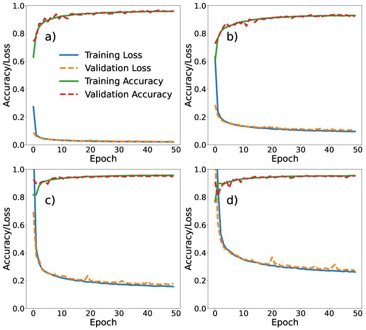
Figure 8: The CNN training progression for (a) $M=2$ (b) $M=4$ (c) $M=6$ (d) $M=8$ in region $k_{i}a\in[0.35,0.45]$. We used the Adam optimizer with a $0.001$ learning rate and mean squared error as the loss function. Each epoch was trained on a small batch of the data with size of either $128$ or $256$ samples, depending on the numbers of cylinders, larger batch size and smaller learning rate is necessary to prevent over fitting. The top two curves show the training and validation accuracy, along with the losses at the bottom two curves.

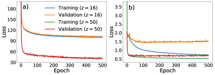
Figure 9: SAVE losses for (a) the reconstruction task and (b) the TSCS regression task for training in the region $ka\in[0.35,0.45]$ when $M=8$. The TSCS regression loss tends to converge faster than the reconstruction loss, however, it shows signs of overfitting. Both losses are much lower when training with a larger $l_{z}$.

References

- [1] Kadic, M., Bückmann, T., Schittny, R., Wegener, M.: Metamaterials beyond electromagnetism. Rep. Prog. Phys. 76(12), 126501 (2013). doi:10.1088/0034-4885/76/12/126501
- [2] Méjica, G.F., Lantada, A.D.: Comparative study of potential pentamodal metamaterials inspired by Bravais lattices. Smart Mat. Struct. 22(11), 115013 (2013). doi:10.1088/0964-1726/22/11/115013
- [3] Su, X., Norris, A.N.: Focusing, refraction, and asymmetric transmission of elastic waves in solid metamaterials with aligned parallel gaps. The Journal of the Acoustical Society of America 139(6), 3386–3394 (2016). doi:10.1121/1.4950770
- [4] Titovich, A.S., Norris, A.N.: Acoustic poisson-like effect in periodic structures. The Journal of the Acoustical Society of America 139(6), 3353–3356 (2016). doi:10.1121/1.4950709
- [5] Packo, P., Norris, A.N., Torrent, D.: Metaclusters for the full control of mechanical waves. Physical Review Applied 15(1) (2021). doi:10.1103/physrevapplied.15.014051
- [6] Norris, A.N.: Acoustic cloaking theory. Proc. R. Soc. A 464, 2411–2434 (2008). doi:10.1098/rspa.2008.0076
- [7] Amirkulova, F.A., Norris, A.N.: The gradient of total multiple scattering cross-section and its application to acoustic cloaking. Journal of Theoretical and Computational Acoustics, 1950016 (2020). doi:10.1142/s2591728519500166
- [8] Titovich, A.S., Norris, A.N., Haberman, M.R.: A high transmission broadband gradient index lens using elastic shell acoustic metamaterial elements. Journal of the Acoustical Society of America 139, 3357–3364 (2016). doi:10.1121/1.4948773
- [9] Fahey, L., Amirkulova, F., Norris, A.: Broadband acoustic metamaterial design using gradient-based optimization. The Journal of the Acoustical Society of America 146(4), 2830–2830 (2019). doi:10.1121/1.5136806
- [10] Haberman, M.R., Guild, M.D., Alù, A.: Acoustic cloaking with plasmonic shells. In: Craster, R.V., Guenneau, S. (eds.) Acoustic Metamaterials. Springer Series in Materials Science, vol. 166, pp. 241–265. Springer, New York London (2013)
- [11] Andkjær, J., Sigmund, O.: Topology optimized cloak for airborne sound. Journal of Vibration and Acoustics 135, 041011 (2013)
- [12] Håkansson, A., Torrent, D., Cervera, F., Sánchez-Dehesa, J.: Directional acoustic source by scattering acoustical elements. Appl. Phys. Lett. 90(22), 224107 (2007). doi:10.1063/1.2743947
- [13] Saanchez-Dehesa, J., Garcia-Chocano, V.M., Torrent, D., Cervera, F., Cabrera, S., Simon, F.: Noise control by sonic crystal barriers made of recycled materials. J. Acoust. Soc. Am. 129(3), 1173 (2011). doi:10.1121/1.3531815
- [14] Andersen, P., Henriquez, V., Sanchis, L., Sánchez-Dehesa, J.: Design of multi-directional acoustic cloaks using two-dimensional shape optimization and the boundary element method. In: Proc. of ICA 2019 AND EAA EUROREGIO Deutsche Gesellschaft Für Akustik e.V., pp. 5600–5606 (2019). Department of Electrical Engineering, Acoustic Technology, Technical University of Denmark
- [15] Campbell, S., Sell, D., Jenkins R., E. Whiting, Fan, J., Werner, D.: Review of numerical optimization techniques for meta-device design [invited]. Optical Materials Express 9(4), 1842–1863 (2019)
- [16] Elsawy, M.M.R., Lanteri, S., Duvigneau, R., Fan, J.A., Genevet, P.: Numerical optimization methods for metasurfaces. Laser & Photonics Reviews 14(10), 1900445 (2020). doi:10.1002/lpor.201900445
- [17] Barrett, R., Chakraborty, M., Amirkulova, D., Gandhi, H., White, A.: A GPU-accelerated machine learning framework for molecular simulation: Hoomd-blue with TensorFlow. 10.26434/chemrxiv.8019527 (2019). doi:10.26434/chemrxiv.8019527
- [18] Elton, D.C., Boukouvalas, Z., Fuge, M.D., Chung, P.W.: Deep learning for molecular design—a review of the state of the art. Molecular Systems Design & Engineering 4(4), 828–849 (2019). doi:10.1039/c9me00039a
- [19] Tahersima, M.H., Kojima, K., Koike-Akino, T., Jha, D., Wang, B., Lin, C., Parsons, K.: Deep neural network inverse design of integrated photonic power splitters. Scientific Reports 9(1), 1368 (2019). doi:10.1038/s41598-018-37952-2
- [20] So, S., Badloe, T., Noh, J., Rho, J., Bravo-Abad, J.: Deep learning enabled inverse design in nanophotonics. Nanophotonics 9(5), 1041–1057 (2020). doi:10.1515/nanoph-2019-0474
- [21] Gurbuz, C., Kronowetter, F., Dietz, C., Eser, M., Schmid, J., Marburg, S.: Generative adversarial networks for the design of acoustic metamaterials. The Journal of the Acoustical Society of America 149(2), 1162–1174 (2021). doi:10.1121/10.0003501
- [22] Shah, T., Zhuo, L., Lai, P., Rosa-Moreno, A.D.L., Amirkulova, F., Gerstoft, P.: Reinforcement learning applied to metamaterial design. Journal of the Acoustical Society of America 150(1) (2021 https://doi.org/10.1121/10.0005545). doi:10.1121/10.0005545
- [23] Wu, R.-T., Liu, T.-W., Jahanshahi, M.R., Semperlotti, F.: Design of one-dimensional acoustic metamaterials using machine learning and cell concatenation. Structural and Multidisciplinary Optimization 63(5), 2399–2423 (2021). doi:10.1007/s00158-020-02819-6
- [24] Wu, R.-T., Jokar, M., Jahanshahi, M.R., Semperlotti, F.: A physics-constrained deep learning based approach for acoustic inverse scattering problems. Mechanical Systems and Signal Processing 164, 108190 (2022). doi:10.1016/j.ymssp.2021.108190
- [25] Ahmed, W.W., Farhat, M., Zhang, X., Wu, Y.: Deterministic and probabilistic deep learning models for inverse design of broadband acoustic cloak. Physical Review Research 3(1) (2021). doi:10.1103/physrevresearch.3.013142
- [26] Jenison, R.L.: A spherical basis function neural network for approximating acoustic scatter. Journal of the Acoustical Society of America 99(5) (1996)
- [27] Jenison, R.L.: Models of direction estimation with spherical-function approximated cortical receptive fields. In: Poon, P., Brugge, J. (eds.) Central Auditory Processing and Neural Modeling, pp. 161–17. Plenum Press, New York (1998)
- [28] Hesham, M., El-Gamal, M.: Neural network model for solving integral equation of acoustic scattering using wavelet basis. Commun. Numer. Meth. Engng 24, 183–194 (2008)
- [29] Hesham, M., El-Gamal, M.: Neural-network solution of the nonuniqueness problem in acoustic scattering using wavelets,. Int. J. for Comp.l Methods in Engng Science and Mech. 9(4), 217–222 (2008). doi:10.1080/15502280802069970
- [30] Gnecco, G., Bacigalupo, A., Fantoni, F., Selvi, D.: Principal component analysis applied to gradient fields in band gap optimization problems for metamaterials. arXiv:2104.02588 [cs.CE] (2021). 2104.02588v2
- [31] Fan, Z., Vineet, V., Gamper, H., Raghuvanshi, N.: Fast acoustic scattering using convolutional neural networks. In: ICASSP 2020 - 2020 IEEE International Conference on Acoustics, Speech and Signal Processing (ICASSP), pp. 171–175 (2020). doi:10.1109/ICASSP40776.2020.9054091
- [32] Fan, Z., Vineet, V., Lu, C., Wu, T.W., McMullen, K.: Prediction of object geometry from acoustic scattering using convolutional neural networks. arXiv:2010.10691 (2021). 2010.10691v3
- [33] Meng, P., Su, L., Yin, W., Zhang, S.: Solving a kind of inverse scattering problem of acoustic waves based on linear sampling method and neural network. Alexandria Engineering Journal 59(3), 1451–1462 (2020). doi:10.1016/j.aej.2020.03.047
- [34] Goodfellow, I.J., Pouget-Abadie, J., Mirza, M., Xu, B., Warde-Farley, D., Ozair, S., Courville, A., Bengio, Y.: Generative adversarial nets. In: Advances in Neural Information Processing Systems 27 (NIPS 2014) (2014). doi:arXiv:1411.1784v1
- [35] Kingma, D.P., Rezende, D.J., Mohamed, S., Welling, M.: Semi-supervised learning with deep generative models. https://arxiv.org/abs/1406.5298 (2014). 1406.5298v2
- [36] Ma, W., Cheng, F., Xu, Y., Wen, Q., Liu, Y.: Probabilistic representation and inverse design of metamaterials based on a deep generative model with semi-supervised learning strategy. Advanced Materials 31(35), 1901111 (2019). doi:10.1002/adma.201901111
- [37] Martin, P.A.: Multiple Scattering: Interaction of Time-harmonic Waves with N Obstacles. Cambridge University Press, New York (2006)
- [38] Norris, A.N.: Acoustic integrated extinction. Proc. R. Soc. A 471(2177), 20150008 (2015). doi:10.1098/rspa.2015.0008
- [39] Amirkulova, F.A.: Acoustic and elastic multiple scattering and radiation from cylindrical structures. PhD thesis, Rutgers University, Piscataway, NJ, USA (2014)
- [40] Kingma, M. D. Welling: Auto-encoding variational bayes. arXiv:1312.6114v10 (2014). doi:arXiv:1312.6114v10 [
- [41] Kingma, D.P., Rezende, D.J., Mohamed, S., Welling, M.: Semi-Supervised Learning with Deep Generative Models (2014). 1406.5298
- [42] Sohn, K., Lee, H., Yan, X.: Learning structured output representation using deep conditional generative models. Advances in neural information processing systems 28, 3483–3491 (2015)
- [43] Osborne, M.A., Garnett, R., Roberts, S.J.: Gaussian processes for global optimization. In: in LION (2009)
- [44] M. Abadi, et al., TensorFlow: Large-scale machine learning on heterogeneous systems (2015). Software available from tensorflow.org.