A Framework for Causal Segmentation Analysis with Machine Learning in Large-Scale Digital Experiments

Abstract

We present an end-to-end methodological framework for causal segment discovery that aims to uncover differential impacts of treatments across subgroups of users in large-scale digital experiments. Building on recent developments in causal inference and non/semi-parametric statistics, our approach unifies two objectives: (1) the discovery of user segments that stand to benefit from a candidate treatment based on subgroup-specific treatment effects, and (2) the evaluation of causal impacts of dynamically assigning units to a study’s treatment arm based on their predicted segment-specific benefit or harm. Our proposal is model-agnostic, capable of incorporating state-of-the-art machine learning algorithms into the estimation procedure, and is applicable in randomized A/B tests and quasi-experiments. An open source R package implementation, sherlock, is introduced.

1 Introduction

The ease and continued improvement in the development and deployment of digital experiments across a variety of platforms has allowed researchers access to cohorts larger and more diverse than previously possible. Whether in randomized experiments or quasi-experiments (i.e., observational studies), a candidate treatment or intervention under investigation hardly ever exhibits a uniform effect across all units enrolled in a study. Typically, studies reveal causal effects that differentially impact segments, or subgroups, of enrolled units, with treatments benefiting a subset of units while posing harm to, or having no effect upon, others — possibly unfairly impacting sensitive groups or yielding benefits too limited to justify the costs associated with deploying the treatment at scale.

At Netflix, most product changes are liable to result in differential impacts across segments of our diverse and growing global user-base of over 200M. Whether the experimental changes are to streaming algorithms, the application’s user interface, or outreach to users, the causal effects of treatments of interest may vary strongly across such user characteristics as viewing habits, the type of viewing device, household make-up, or global region, to name but a few. Providing the best experience for all of our users and ensuring the equitability of treatment allocation in our digital experiments is imperative to the continuous improvement of our platform; moreover, understanding treatment effect heterogeneity across segments of our eclectic user-base plays a critical role in our product improvement endeavors.

Recent developments in causal inference, studying estimation of conditional treatment effects and the population-level causal effects of dynamically assigning treatments based on units’ characteristics [15] have provided novel statistical techniques that may be unified into a single framework for both discovering population segments benefiting from a treatment [10] and evaluating the causal effects of dynamic treatment rules that assign to the treatment arm only those segments predicted to benefit [11]. Notably, these recent statistical advances have been formulated in a manner capable of incorporating state-of-the-art machine learning algorithms in the estimation procedure while simultaneously fulfilling the theoretical requirements for valid statistical inference on the estimated treatment effects [9].

The remainder of this manuscript is organized as follows. In Section 2, we review the foundations of a statistical framework for identifying population segments based upon treatment effect heterogeneity and estimating the causal effects of dynamic treatment rules assigned based upon the conditional average treatment effect. Section 3 describes sherlock, a software package we designed to allow our data scientists to perform causal machine learning for population segment discovery and analysis. In Section 4, we present an illustrative example of applying our causal segment discovery framework, and the sherlock package, to analyzing synthetic data inspired by quasi-experiments at Netflix.

2 A Causal Segment Discovery Framework

We consider the problem of discovering segments of users that should benefit from a given treatment subject to an optimality criterion. More precisely, for a dataset collected in a randomized A/B test or in a quasi-experiment, we measure baseline covariates $W$, the assigned treatment $A$, and response/outcome $Y$ on a set of $n$ units. We additionally assume access to a set of segmentation covariates $V$ that temporally precede treatment assignment (and, thus, are unaffected by it), with which we aim to segment the population. This set of segmentation covariates may be high-dimensional (i.e., consisting of many covariates), have high cardinality (i.e., a large support space for at least a single covariate), or both. We define a segment as a particular realization of these covariates (i.e., $V=v$). The segmentation covariates are often a subset of the baseline covariates (i.e., $V\subset W$), which, in the case of non-randomized studies, may be used to adjust for confounding of the treatment-outcome relationship, or, in A/B tests, to reduce estimation variance by covariate adjustment. For a given segment $V=v$, the conditional average treatment effect (CATE) on this segment is given by $\text{CATE}(v)=\mathbb{E}[\mathbb{E}(Y\mid A=1,W)-\mathbb{E}(Y\mid A=0,W)\mid V=v]$.

The goal of segment discovery is to reveal which segments ought to benefit from treatment, with the possible benefit being defined in two distinct ways, as enumerated below.

1. In absolute terms, where the goal is to identify segments whose $\text{CATE}(v)$ estimates fall above a user-specified benefit threshold $\theta$, i.e., $T=\{v:\text{CATE}(v)>\theta\}$.

2. Subject to cost or side-effect constraints, which can be formulated as a constrained optimization problem with respect to the CATE. Specifically, the goal in this case is to identify a set of segments $T$ so as to maximize the population-level outcome

   $$\psi=\sum_{v\in T}\mathbb{E}[\mathbb{E}(Y\mid A=1,W)\mid V=v]p(v)+\sum_{v\notin T}\mathbb{E}[\mathbb{E}(Y\mid A=0,W)\mid V=v]p(v),$$ (1)

   subject to a cost constraint $\sum_{v\in T}\text{Cost}(v)p(v)\leq\phi$. Here, $\text{Cost}(v)\geq 0$ is the known cost of treating a unit in a given segment, the budget $\phi$ is a given spending cap, and $p(v)$ is the marginal distribution of segment $v$ in the population. This is equivalent to the binary knapsack problem of finding $T\subseteq\{v:\text{CATE}(v)>0\}$ such that we maximize $\sum_{v\in T}\text{CATE}(v)$ while respecting the constraint $\sum_{v\in T}\text{Cost}(v)p(v)\phi$.

Estimation of the CATE requires the use of sample splitting principles in order to avoid overfitting that stems from learning the dynamic treatment rule and evaluating the population-level causal effects of the learned rule within a single study cohort [13]. Similar principles were studied in the formulation of cross-validated targeted minimum loss estimation (CV-TMLE) [16], have recently been renamed “cross-fitting” [3], and appeared decades ago in studies of efficient estimation in semiparametric models [7, 2]. Following the partitioning of the dataset into $K$ training and validation folds (i.e., $K$-fold cross-validation), we apply user-specified machine learning algorithms to obtain out-of-sample (or holdout) predictions of the outcome regression $\hat{\mathbb{E}}_{Y}(Y\mid A,W)$, the conditional mean of the outcome given observed treatment status and covariates, and of the propensity score $\hat{p}_{A}(A\mid W)$, the conditional probability of treatment assignment given covariates. Next, using the form of the efficient influence function [2], a central quantity in semiparametric theory, a doubly robust outcome transformation may be applied to obtain the pseudo-outcome $\hat{D}=[(2A-1)/\hat{\mathbb{P}}_{A}(A\mid W)]\cdot[Y-\hat{\mathbb{E}}_{Y}(Y\mid A,W)]+\hat{\mathbb{E}}_{Y}(Y\mid 1,W)-\hat{\mathbb{E}}_{Y}(Y\mid 0,W)$. Regressing the outcome $\hat{D}$ on segmentation covariates $V$, by way of another user-specified machine learning algorithm, yields $\hat{\mathbb{E}}_{V}(\hat{D}\mid V)$, a doubly robust estimator of $\text{CATE}(v)$, which admits analytical standard error calculations based on its efficient influence function. For both problems (1) and (2), a single-tailed test of the null and alternative hypotheses $\{H_{0}:\text{CATE}(v)\leq\theta,H_{1}:\text{CATE}(v)>\theta\}$, across the segments can be used to assign the treatment rule inferentially, with multiple comparisons corrections to account for the number of segments. For problem (2), only segments for which $\text{CATE}(v)>0$ (i.e., those expected to benefit from treatment) are considered as candidates in the binary knapsack problem.

After learning the segments that should receive treatment, we can assess the gain attributable to such dynamic treatment strategies, by comparison against a global (or “one-size-fits-all”) treatment strategy. A dynamic treatment strategy learned in this way is defined as a function $A=d(v)$, where $d(v)$ is the indicator that $v\in T$, that is, whether a given user belongs to a “should-treat” segment. At this point, doubly robust estimators of optimal treatment effects (OTEs), such as $\psi_{\text{OTE}}=\mathbb{E}[\mathbb{E}(Y\mid A=d(V),W)-\mathbb{E}(Y\mid A=1,W)]$, or the heterogeneous treatment effect (HTE) over the segments, namely, $\psi_{\text{HTE}}=\mathbb{E}[\mathbb{E}(Y\mid A=1,W)-\mathbb{E}(Y\mid A=0,W)\mid V\in T]-\mathbb{E}[\mathbb{E}(Y\mid A=1,W)-\mathbb{E}(Y\mid A=0,W)\mid V\notin T]$, may be used to evaluate the quality of the population segmentation based on the expected utility of deploying the resultant dynamic treatment strategy.

3 sherlock: A Modular and Scalable Software Implementation

We developed sherlock, a software package for the R programming language and environment for statistical computing [12], to simplify the use of our causal segmentation framework in both randomized A/B testing and quasi-experimental study settings. The design of this R package emphasized two key goals: modularity and scalability. In terms of modularity, the package abstracts the causal segmentation analysis pipeline into three broad steps, each representing a distinct point of analytical interest and encoded in one of sherlock user-facing wrapping functions.

1. Evaluate treatment effect heterogeneity across the segment groups, requiring estimation of nuisance parameters as well as estimation of the CATE on the population segments $v\in V$. This step involves computing estimates of the propensity score, the outcome regression, and of $\text{CATE}(v)$, for which a user-specified modeling algorithm (or algorithm library) is used. In particular, we recommend the Super Learner algorithm, which allows the selection of a single algorithm (or the construction of an ensemble model) from a user-specified algorithm library, using loss-based cross-validation to achieve optimal asymptotic performance [14]. To facilitate access to a wide variety of modeling algorithms, sherlock is tightly coupled with the open source sl3 R package [5], which acts both as an interface to 50+ machine learning algorithms and a standalone implementation of the Super Learner algorithm. This step is encoded in the sherlock_calculate() function.

2. Dynamically assign treatment to (or withhold treatment from) the population segments, based on options for evaluating treatment efficacy, including thresholding the CATE at a user-given cutoff or while accounting for an overall budget or cost for deploying the treatment [8, 15]. This step uses the estimated $\text{CATE}(v)$ and user-specified optimality criterion (e.g., total budget) to assign segments with $\text{CATE}(v)>0$ to the treatment arm, constructing confidence intervals and performing hypothesis tests (i.e., $H_{0}:\text{CATE}(v)\leq\theta,H_{1}:\text{CATE}(v)>\theta$). The data scientist may now examine a summary of the segmentation results (see Table 2), which includes segment identifiers $v\in V$, point estimates of $\text{CATE}(v)$, inference for the estimates, and an indication of a segment’s treatment assignment (i.e., $v\in T$). This is implemented by the watson_segment() function.

3. Estimate population-level causal effects of the dynamic treatment rule, including both HTEs, which contrast the effects of the intervention within the treatment allocations derived in the preceding step, and OTEs, which contrast counterfactual means under the dynamic treatment rule with those of static treatment strategies. This step allows for the evaluation of segmentation quality through the use of non/semi-parametric efficient estimation of the effect measures discussed in Section 2. Notably, neither this step nor the preceding step is computationally demanding, relying primarily on the nuisance estimates generated in the first step. These effects are computed by the mycroft_assess() function.

With respect to scalability, sherlock’s design emphasized enumerating the set of nuisance functionals required for doubly robust estimation of the CATE and the causal effect measure parameters (i.e., HTE, OTE). By accounting for dependencies across stages of the estimation procedure at the design stage, sherlock’s pipeline collapses computationally taxing nuisance regressions into a single step, thereby streamlining the latter steps, in which the segment-specific treatment rule is assigned and the quality of segmentation evaluated. This reduced computational burden is a direct result of (1) avoiding redundant computation and (2) breaking dependencies between steps of the estimation routine to introduce modularization. Together, these design choices allow the data science practitioner increased flexibility when using sherlock to perform causal segmentation analysis, allowing for choices of the treatment rule optimality criterion and effect measure to be siloed entirely from nuisance estimation — that is, the nuisance estimate “building blocks” may easily be extracted and manipulated, without any need for re-computation, as the analytical decision-making process progresses.

Finally, sherlock includes (by way of sl3) facilities to introduce customizable wrappers that accommodate newly developed machine learning algorithms or regression techniques for the estimation of nuisance parameters. In our application settings — working with large-scale experiments with millions of users — this proves an important point of flexibility, as regression algorithms do not uniformly scale to massive sample sizes. Instead, the analyst may, with little overhead, build bindings for algorithms optimized to the scale and characteristics of the dataset at hand, including, for example, algorithms optimized to respect measurement sparsity. To support cross-validation of nuisance estimates, sherlock relies on the origami R package [4], which provides a general and flexible framework for sample splitting. Both origami and sl3 utilize the Future framework [1] for delayed and parallelized computation in R, allowing sherlock to take full advantage of available compute resources; moreover, sherlock’s data structures are simple instantiations of R’s data.table [6], which provides numerous optimizations that streamline computation, including reference assignment operations that curb memory usage, helpful when working with massive datasets. An open source release of our sherlock R package is available on GitHub at https://github.com/Netflix/sherlock, and, in time, sherlock will additionally be made available via the Comprehensive R Archive Network (CRAN).

4 Illustrative Example

We demonstrate the use of our causal segment discovery framework by the application of sherlock to a synthetic dataset example inspired by quasi-experiments at Netflix. In our simulated dataset, we have $n=5000$ independent units (e.g., Netflix accounts), upon which we have measured $7$ variables, including the number of devices associated with a given account (“num_devices”), whether the account belongs to a newly enrolled Netflix member (“is_p2plus”), whether the account is located in a new market region (“is_newmarket”), the account’s estimated lifetime value (“baseline_ltv”), a measure of the account’s baseline viewing hours (“baseline_viewing”), non-randomized assignment to a new user interface (UI; the treatment), and a measure of post-treatment Netflix viewing hours (“outcome_viewing”). A few randomly selected rows of the dataset appear in Table 1 for reference.

num_devices	is_p2plus	is_newmarket	baseline_ltv	baseline_viewing	treatment	outcome_viewing
3	0	1	0.539	0.000	1	0.406
2	1	1	1.328	1.637	0	2.328
3	1	0	0.000	0.000	1	3.400
2	1	0	1.027	0.000	0	1.934
2	1	1	0.000	0.000	0	1.376
3	0	1	0.000	1.401	0	2.683

Table 1: Measurements collected on six units in a simulated quasi-experimental dataset. Assessing the impact of the new UI, itself possibly affected by the baseline covariates, on the outcome of viewing hours is the question of interest.

The candidate segmentation covariates are the number of devices associated with the account and whether the account belongs to a new member. Across these two segmentation covariates, we observe $10$ strata, that is, $\text{card}(V)=10$. Next, we evaluate treatment effect heterogeneity by estimating the CATE, using a handful of regression and machine learning algorithms to fit nuisance parameters. By calling the function sherlock_calculate() and its associated plotting method, we can easily visualize the CATE estimates across each segment; these are displayed in Figure 1.

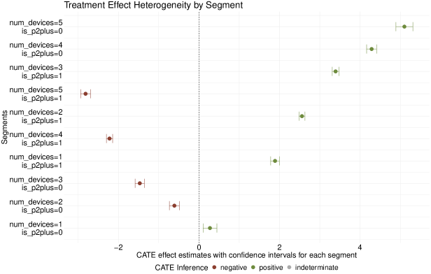
Figure 1: Results of causal segmentation analysis, with statistical inference for the CATE. Deploying the new UI is expected to lower the viewing hours of segments with negative CATE estimates, while yielding increases in viewing hours for those segments with positive estimates.

With CATE estimates for each population segment, we are now prepared to decide which subgroups ought to have the new UI experience rolled out to them. Using sherlock’s watson_segment() function, we can evaluate the evidence for a segment benefiting from treatment, thresholding the CATE at its null value of $\theta=0$ (i.e., no treatment effect) and correcting for hypothesis testing multiplicity appropriately; the results are summarized in Table 2.

num_devices	is_p2plus	Segment Proportion	CATE	Lower CL	Upper CL	Std. Err.	p-value	Treat?
1	0	0.0392	0.283	0.108	0.459	0.089	0.001	Yes
1	1	0.0862	1.895	1.787	2.00	0.055	0.000	Yes
2	0	0.0718	-0.595	-0.719	-0.471	0.063	1.000	No
2	1	0.1752	2.550	2.473	2.626	0.039	0.000	Yes
3	0	0.0764	-1.462	-1.580	-1.343	0.061	1.000	No
3	1	0.1796	3.391	3.308	3.473	0.042	0.000	Yes
4	0	0.0728	4.304	4.180	4.428	0.063	0.000	Yes
4	1	0.1814	-2.214	-2.291	-2.137	0.039	1.000	No
5	0	0.0328	5.094	4.879	5.310	0.119	0.000	Yes
5	1	0.0846	-2.798	-2.921	-2.674	0.063	1.000	No

Table 2: Point estimates of $\text{CATE}(v)$, with lower and upper confidence limits across the ten segments, as well as p-values for hypothesis tests of $H_{0}:\text{CATE}(v)\leq\theta,H_{1}:\text{CATE}(v)>\theta$ and corresponding treatment decisions.

Acknowledgements

We thank Simon Ejdemyr and Martin Tingley, for helpful discussions and feedback on an early draft of this manuscript; Stephanie Lane, for helpful guidance on sherlock’s native data visualization capabilities; and Mark van der Laan, for insightful remarks on the implementation of previously described algorithms for targeted minimum loss estimation.

References

- [1] H. Bengtsson, “A Unifying Framework for Parallel and Distributed Processing in R using Futures,” The R Journal, 2021. [Online]. Available: https://journal.r-project.org/archive/2021/RJ-2021-048/index.html
- [2] P. J. Bickel, C. A. Klaassen, Y. Ritov, and J. A. Wellner, Efficient and Adaptive Estimation for Semiparametric Models. Johns Hopkins University Press Baltimore, 1993.
- [3] V. Chernozhukov, D. Chetverikov, M. Demirer, E. Duflo, C. Hansen, and W. Newey, “Double/debiased/neyman machine learning of treatment effects,” American Economic Review, vol. 107, no. 5, pp. 261–65, 2017.
- [4] J. R. Coyle and N. S. Hejazi, “origami: A generalized framework for cross-validation in R,” Journal of Open Source Software, vol. 3, no. 21, p. 512, 1 2018. [Online]. Available: https://doi.org/10.21105/joss.00512
- [5] J. R. Coyle, N. S. Hejazi, I. Malenica, R. V. Phillips, and O. Sofrygin, sl3: Modern Pipelines for Machine Learning and Super Learning, https://github.com/tlverse/sl3, 2021, R package version 1.4.3. [Online]. Available: https://doi.org/10.5281/zenodo.1342293
- [6] M. Dowle and A. Srinivasan, data.table: Extension of “data.frame”, 2021, R package version 1.14.0. [Online]. Available: https://CRAN.R-project.org/package=data.table
- [7] C. A. Klaassen, “Consistent estimation of the influence function of locally asymptotically linear estimators,” The Annals of Statistics, pp. 1548–1562, 1987.
- [8] A. R. Luedtke and M. J. van der Laan, “Optimal individualized treatments in resource-limited settings,” The International Journal of Biostatistics, vol. 12, no. 1, pp. 283–303, 2016.
- [9] ——, “Statistical inference for the mean outcome under a possibly non-unique optimal treatment strategy,” Annals of Statistics, vol. 44, no. 2, p. 713, 2016.
- [10] ——, “Super-learning of an optimal dynamic treatment rule,” The International Journal of Biostatistics, vol. 12, no. 1, pp. 305–332, 2016.
- [11] ——, “Evaluating the impact of treating the optimal subgroup,” Statistical Methods in Medical Research, vol. 26, no. 4, pp. 1630–1640, 2017.
- [12] R Core Team, R: A Language and Environment for Statistical Computing, R Foundation for Statistical Computing, Vienna, Austria, 2021. [Online]. Available: https://www.R-project.org/
- [13] M. J. van der Laan and A. R. Luedtke, “Targeted learning of the mean outcome under an optimal dynamic treatment rule,” Journal of Causal Inference, vol. 3, no. 1, pp. 61–95, 2015.
- [14] M. J. van der Laan, E. C. Polley, and A. E. Hubbard, “Super Learner,” Statistical Applications in Genetics and Molecular Biology, vol. 6, no. 1, 2007.
- [15] T. J. VanderWeele, A. R. Luedtke, M. J. van der Laan, and R. C. Kessler, “Selecting optimal subgroups for treatment using many covariates,” Epidemiology, vol. 30, no. 3, p. 334, 2019.
- [16] W. Zheng and M. J. van der Laan, “Cross-validated targeted minimum-loss-based estimation,” in Targeted Learning: Causal Inference for Observational and Experimental Data. Springer, 2011, pp. 459–474.