Dynamics in a stellar convective layer and at its boundary: Comparison of five 3D hydrodynamics codes

Our ability to predict the structure and evolution of stars is in part limited by complex, 3D hydrodynamic processes such as convective boundary mixing. Hydrodynamic simulations help us understand the dynamics of stellar convection and convective boundaries. However, the codes used to compute such simulations are usually tested on extremely simple problems and the reliability and reproducibility of their predictions for turbulent flows is unclear. We define a test problem involving turbulent convection in a plane-parallel box, which leads to mass entrainment from, and internal-wave generation in, a stably stratified layer. We compare the outputs from the codes FLASH, MUSIC, PPMSTAR, PROMPI, and SLH, which have been widely employed to study hydrodynamic problems in stellar interiors. The convection is dominated by the largest scales that fit into the simulation box. All time-averaged profiles of velocity components, fluctuation amplitudes, and fluxes of enthalpy and kinetic energy are within $\lesssim 3\sigma$ of the mean of all simulations on a given grid ($128^{3}$ and $256^{3}$ grid cells), where $\sigma$ describes the statistical variation due to the flow’s time dependence. They also agree well with a $512^{3}$ reference run. The $128^{3}$ and $256^{3}$ simulations agree within $9\%$ and $4\%$, respectively, on the total mass entrained into the convective layer. The entrainment rate appears to be set by the amount of energy that can be converted to work in our setup and details of the small-scale flows in the boundary layer seem to be largely irrelevant. Our results lend credence to hydrodynamic simulations of flows in stellar interiors. We provide in electronic form all outputs of our simulations as well as all information needed to reproduce or extend our study.

1 Introduction

Convection is the most important mixing process in stars. Due to the high density and opacity deep in the stellar interior, the convection is almost adiabatic and Mach numbers are typically $\mathcal{M}<0.05$ in late evolutionary phases of massive stars and $10^{-4}\lesssim\mathcal{M}\lesssim 10^{-3}$ in early phases, such as core convection during H and He burning. Such slow flows are nearly incompressible in the sense that ram pressure is much smaller than thermal pressure, although significant compression and expansion still occur when fluid packets are displaced radially in the strong, nearly hydrostatic pressure stratification. The spatial scales involved are so large that molecular viscosity is negligible and the flow is highly turbulent. The main effect of convection on the structure and evolution of stars is the transport of species, energy, and angular momentum. The mixing of chemical species has important implications for the generation of nuclear energy, origin of elements, stellar lifetimes, or the observable properties of stars and stellar populations. The physics of convection is key to determining the endpoints of stellar evolution which in turn give rise to some of the most energetic events in the Universe, such as supernova explosions and compact-object mergers.

Despite its importance, the treatment of convective mixing and energy transport is still very rudimentary in stellar-evolution models. This is because the long thermal and nuclear timescales of stellar evolution make 1D, time-averaged models the only practical approach. The mixing-length theory (MLT; Prandtl, 1925; Böhm-Vitense, 1958) is the most common parametric description of convection in stellar-evolution codes. The MLT’s main parameter, the mixing length $\alpha$, is usually calibrated such that the code reproduces current properties of the Sun and $\alpha$ is then assumed to be the same in all convective layers in all stars. Three-dimensional hydrodynamic simulations of near-surface convection show that $\alpha$ varies across the Hertzsprung-Russel diagram (Trampedach et al., 2014; Magic et al., 2015; Sonoi et al., 2019). Trampedach et al. (2014) and Jørgensen et al. (2018) illustrate how such realistic 3D models can be used to replace the MLT in near-surface layers in stellar-evolution calculations. Deep in the stellar interior, which is the main focus of our work, convection is so efficient that the stratification becomes isentropic almost independently of $\alpha$. The MLT is then used to get an estimate of mixing speed, which is important for the stratification of species when the timescale of some nuclear reaction(s) becomes comparable to or shorter than the mixing timescale across the convective layer. Nevertheless, the stellar model remains 1D, and the mixing is usually described as a diffusive process, although alternative approaches are being developed (e.g. Stephens et al., 2021).

The MLT is a local theory and as such it cannot describe any mixing caused by the non-local nature of convection and reaching beyond the formal convective boundary. Traditionally known as ‘convective overshooting’, this mixing may involve a number of distinct physical processes and it is better described by the more general term ‘convective boundary mixing’ (CBM; Denissenkov et al., 2013). CBM enlarges stellar convection zones and it is required to explain a large number of observations such as the position of the turn-off point in open clusters (Rosvick & Vandenberg, 1998), the width of the main sequence in the Hertzsprung-Russell diagram (Castro et al., 2014), properties of double-lined eclipsing binaries (Claret & Torres, 2019, and references therein), or asteroseismic observations of massive stars (Aerts, 2021, and references therein). In calculations of stellar evolution, CBM is added in the form of a simplistic model, such as instantaneous overshooting (Maeder, 1976; Ekström et al., 2012), a diffusive model (Herwig, 2000; Battino et al., 2016; Baraffe et al., 2017), or an entrainment model (Staritsin, 2013; Scott et al., 2021). Each of these formulations has at least one free parameter, which is usually calibrated by comparison with observations. However, there is no reason to expect that the same parameter(s) should apply across different convection zones in different stars at different stages of evolution.

Multiple research groups have started to use 2D and 3D hydrodynamic codes to simulate stellar convection and CBM in order to calibrate free parameters of the CBM models mentioned above, for example, Meakin & Arnett (2007); Jones et al. (2017); Pratt et al. (2017); Cristini et al. (2019); Denissenkov et al. (2019), and Horst et al. (2021). Although the growth rates of convective layers in such simulations seem to be reasonable for late stages of stellar evolution (Meakin & Arnett, 2007; Woodward et al., 2015; Jones et al., 2017; Mocák et al., 2018), they are much too high to be compatible with observations on the main-sequence (Meakin & Arnett, 2007; Gilet et al., 2013; Scott et al., 2021). It is not clear whether this is because the simulations’ parameters are too far from the stellar regime, or it is due to some physics not being included in the simulations, or it is a sign of numerical problems.

Simulations of convection on the main sequence have become even more attractive with the recent boom in asteroseismology. The generation of waves by convection and their propagation through the rest of the star can be observed in 2D and 3D simulations directly, although most codes require an artificial increase in the energy generation rate to speed up the flow. The resulting wave spectra can, in principle, be compared with observations of real stars. However, some groups obtain spectra with many strong resonance lines (Lecoanet et al., 2021) whereas others get featureless, continuous spectra (Alvan et al., 2014; Edelmann et al., 2019; Horst et al., 2020). Again, it is unclear whether the difference can be tracked down to physical assumptions or they are of numerical origin.

Probably all major hydrodynamics codes used in the field have passed a series of tests using problems with known solutions such as shock tubes or various instabilities during their initial growth. However, the stellar hydrodynamic cases that we are interested in are much more complex and exact solutions do not exist. Instead, code verification is done by comparing solutions obtained with different codes. Such exercises have a long tradition in computational dynamics (Joggerst et al., 2014; Ramaprabhu et al., 2012; Dimonte et al., 2004) and also in astrophysics (Doherty et al., 2010; Beeck et al., 2012; McNally et al., 2012; Kim et al., 2014, 2016; Lecoanet et al., 2016; Christensen-Dalsgaard et al., 2020; Silva Aguirre et al., 2020; Fleck et al., 2021). Nonetheless, a test problem focused on the dynamics of convection and mixing processes in stellar interiors has been missing in the literature.

We constructed a complex test problem as detailed in Sect. 2.2. It involves stratified, turbulent convection, and CBM as well as the generation and propagation of internal gravity waves in a plane-parallel box. The presence of turbulence makes this problem fundamentally different from classical test cases such as shock tubes. Even if the initial and boundary conditions are given, the chaotic nature of the flow leads to rapid amplification of small perturbations in numerical simulations as well as in real flows. Nevertheless, many space- and time-averaged quantities are expected to converge upon grid refinement in a statistical way, for instance velocity profiles, spectra, fluxes, or the cumulative amount of CBM. The statistical variation left in these averages descreases as the length of the averaging time interval is increased. However, our test problem, designed to be as close as possible to real science cases, involves continuous heating and mass entrainment. The resulting secular evolution limits the extent of time averaging applicable and we must estimate the magnitude of statistical variation when comparing results of such simulations. Still, we believe that our test problem can be used to compare codes with accuracy appropriate to the current state of the field.

We ran simulations using the codes FLASH, MUSIC, PPMSTAR, PROMPI, and SLH, which have been widely used to study hydrodynamic problems in stellar interiors and are briefly described in Sect. 2.3. The simulations are compared in a number of metrics: velocity amplitudes, profiles, and spectra (Sect. 3.1), properties of the convective boundary and the mass entrainment rate (Sect. 3.2), the amplitudes of fluctuations, and energy fluxes (Sect. 3.3). Finally, we summarise our results in Sect. 4. Our selection of codes for this study is based on collaborative ties and availability of resources and it is far from being unbiased or complete. In particular, our study does not include any finite-difference and spectral schemes. However, we provide our test setup as well as all data-analysis scripts in electronic form for anyone interested in extending this study, see Appendix A.

2 Methods

2.1 Motivation of the oxygen shell test problem

In this study, we aim to define a problem that involves turbulent convection and CBM while being simple enough to be accessible to as many codes as possible. We define our test problem to be similar to the simulations of Jones et al. (2017) and Andrassy et al. (2020) of shell oxygen burning in a massive star. The stratification of the underlying stellar model is compared with that of our test problem (specified in Sect. 2.2) in Fig. 1. Although the oxygen shell is spherical, we use plane-parallel geometry both for simplicity and to reduce computational costs. The lower half of the simulation domain is initially isentropic and the upper half is stably stratified and approximately follows the density stratification of the stellar model. Because we intend to study the dynamics of a single convective boundary in isolation, we do not include the convective carbon-burning shell, the bottom of which corresponds to the discontinuity at $r\approx 2.35$ in the stellar model.

To further simplify the problem, we follow Jones et al. (2017) and Andrassy et al. (2020) and use the ideal-gas equation of state, neglect neutrino cooling, and replace nuclear reactions with a constant and easy-to-resolve heating profile. Compared with the original stellar model, the total luminosity driving convection is $22.5$ times larger and the convective layer contains, due to its different geometry, $5.4$ times less mass. The resulting rms Mach number of the convective flow is then ${\approx}\,0.04$, making the problem well accessible to explicit and implicit codes as well as to codes using low-Mach approximations. Molecular viscosity, thermal conduction, and radiative diffusivity are not considered.

We adopt the speed of sound, density, and temperature at the bottom of the convective layer as units of velocity, density, and temperature, respectively, and we take the approximate depth of the convective layer to be the unit of length. The numerical values of these units as well as those of other units derived from them are summarised in Table 1. The dimensionless problem is specified in detail in the following section.

2.2 Problem specification

Table 1: Basic problem units (upper section), derived units (middle section), and adopted values of physical constants (lower section).

Quantity	Unit
density	$1.820940\times 10^{6}$	g cm-3
length	$4.000000\times 10^{8}$	cm
temperature	$3.401423\times 10^{9}$	K
velocity	$5.050342\times 10^{8}$	cm s-1
acceleration	$6.376489\times 10^{8}$	cm s-2
energy	$2.972468\times 10^{49}$	erg
luminosity	$3.752995\times 10^{49}$	erg s-1
mass	$1.165402\times 10^{32}$	g
pressure	$4.644481\times 10^{23}$	dyn cm-2
time	$7.920256\times 10^{-1}$	s
volume	$6.400000\times 10^{25}$	cm3
atomic mass unit	$1.660539\times 10^{-24}$	g
Boltzmann constant	$1.380649\times 10^{-16}$	erg K-1
gas constant	$8.314463\times 10^{7}$	erg g-1 K-1
gravitational constant	$6.674300\times 10^{-8}$	dyn cm2 g-2

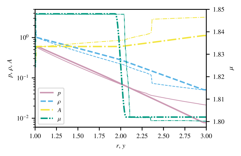
Figure 1: Initial stratification in the problem units (Table 1) of the pressure $p$, density $\rho$, pseudo-entropy $A=p/\rho^{\gamma}$, and mean molecular weight $\mu$ in the stellar model (thin lines) and in the test problem (thick lines). The discontinuity visible in the stellar model at $r\approx 2.35$ is the bottom of the carbon-burning shell, which is not included in our test problem.

The initial hydrostatic stratification, shown in Fig. 1, is computed using the following profile of gravitational acceleration:

$$g(y)=g_{0}\,f_{g}(y)\,y^{-5/4},$$ (1)

where $g_{0}=1.414870$ is the gravitational acceleration at the bottom of the oxygen-burning shell in the stellar model. The vertical coordinate $y$ runs from $1$ to $3$, which in principle allows the same stratification to be used in spherical coordinates simply by setting the radius $r=y$. This profile is similar to the stellar one and the reduction in gravity with height helps prevent a too-fast decrease in the pressure scale height. We ‘turn off’ gravity close to the lower and upper boundaries of the simulation domain using the factor

$$f_{g}(y)=\cases{}{1}{2}\left\{1+\sin\left[16\pi\left(y-\frac{1}{32}\right)\right]\right\},&\mathrm{for}\ 1\leq y<1+\frac{1}{16},\\ 1,\mathrm{for}\ 1+\frac{1}{16}\leq y\leq 3-\frac{1}{16},\\ \frac{1}{2}\left\{1+\sin\left[16\pi\left(y-\frac{1}{32}\right)\right]\right\},\mathrm{for}\ 3-\frac{1}{16}<y\leq 3,{}$$ (2)

which forces density and pressure to become constant close to the boundaries and thus makes possible the use of a simple reflective boundary condition there. The computational domain contains a mixture of two monatomic ideal gases with $\gamma=5/3$ and mean molecular weights of $\mu_{0}=1.848$ and $\mu_{1}=1.802$. Initially, the convective layer is filled with the $\mu_{0}$ fluid and the stable layer with the $\mu_{1}$ fluid. There is a smooth transition between the two layers and the fractional volume $\eta_{1}$ of the $\mu_{1}$ fluid varies as

$$\eta_{1}(y)=\cases{0},&\mathrm{for}\ 1\leq y<2-\frac{1}{16},\\ \frac{1}{2}\left[1+\sin\left(8\pi y\right)\right],\mathrm{for}\ 2-\frac{1}{16}\leq y\leq 2+\frac{1}{16},\\ 1,\mathrm{for}\ 2+\frac{1}{16}<y<3.{}$$ (3)

The mixture is assumed to be in local pressure and thermal equilibrium everywhere and the stratification follows the piecewise-polytropic pressure-density relation

$$\frac{\mathrm{d}\ln p}{\mathrm{d}\ln\rho}=\cases{\gamma}_{0},&\mathrm{for}\ 1\leq y<2-\frac{1}{16},\\ \gamma_{0}+\eta_{1}(y)(\gamma_{1}-\gamma_{0}),\mathrm{for}\ 2-\frac{1}{16}\leq y\leq 2+\frac{1}{16},\\ \gamma_{1},\mathrm{for}\ 2+\frac{1}{16}<y<3,{}$$ (4)

where $\gamma_{0}=\nicefrac{{5}}{{3}}$ and $\gamma_{1}=1.3$. Equations 1 – 4, together with the ideal-gas law define a unique hydrostatic state.

We impose friction-free, non-conductive wall boundary conditions at $y=1$ and $y=3$. The specific implementation of these boundary conditions is code-dependent, see Sect. 2.3. The computational domain is periodic in the two horizontal dimensions and spans the coordinate intervals $-1\leq x\leq 1$ and $-1\leq z\leq 1$. The initial aspect ratio of the convective layer is thus $2{:}1$ (width to height).

Convection is driven using a time-independent heat source concentrated close to the lower boundary of the convective layer with energy generation rate per unit volume of

$$\dot{q}(y)=\cases{\dot{\hfil}}{q}_{0}\sin\left(8\pi y\right),&\mathrm{for}\ 1\leq y\leq 1+\frac{1}{8},\\ 0,\mathrm{for}\ 1+\frac{1}{8}<y\leq 3,{}$$ (5)

where $\dot{q}_{0}=3.795720\times 10^{-4}$. The total luminosity of the heat source is $1.2082151\times 10^{-4}$. When the problem is discretised, we take into account the fact that the average value of $\dot{q}(y)$ over a computational cell of height $\Delta y$ centred around $y=y_{0}$ is $\dot{q}(y_{0})\sin(4\pi\Delta y)/(4\pi\Delta y)$. The heat source is defined to be smooth and easy to resolve for this study; the energy generation profile in the stellar model is asymmetric and discontinuous (see Fig. 3 of  Jones et al., 2017). We do not include any cooling term. The Kelvin-Helmholtz timescales of the convective layer and of the whole computational domain are $1.29\times 10^{4}$ and $1.43\times 10^{4}$ time units, respectively.

To break the initial symmetry, we use a density perturbation

$$\frac{\Delta\rho}{\rho_{0}}=5\times 10^{-5}\,\frac{\dot{q}(y)}{\dot{q}_{0}}\left[\sin(3\pi x)+\cos(\pi x)\right]\left[\sin(3\pi z)-\cos(\pi z)\right],$$ (6)

where $\rho_{0}=1$ is the density at the bottom of the convective layer. The perturbation only affects the heating layer, so it is also concentrated close to the lower boundary of the convective layer. There is no pressure perturbation. The smooth density perturbation, although small, allows us to produce a well-resolved initial transient, which should be similar in all codes.

The problem is described by the inviscid Euler equations with gravity and volume heating,

$$\frac{\partial\rho}{\partial t}+\bm{\nabla}\cdot(\rho\bm{V}) =0,$$ (7)

$$\frac{\partial(\rho\bm{V})}{\partial t}+\bm{\nabla}\cdot(\rho\bm{V}\otimes\bm{V}+p\bm{I}) =\rho\bm{g},$$ (8)

$$\frac{\partial(\rho E)}{\partial t}+\bm{\nabla}\cdot[(\rho E+p)\bm{V}] =\rho\bm{V}\cdot\bm{g}+\dot{q},$$ (9)

where $\bm{V}$ is the velocity vector, $\bm{I}$ the unit tensor, $\bm{g}$ the gravitational acceleration vector pointed towards the negative $y$ axis, and $E=e+\frac{1}{2}\|\bm{V}\|^{2}$ the specific total energy, which includes the specific internal energy $e$ and the specific kinetic energy $\frac{1}{2}\|\bm{V}\|^{2}$. Some of our codes, as indicated in Table 2, include the specific potential energy $\Phi$ in the total energy $E_{\Phi}=E+\Phi$ and, instead of evolving Eq. 9, they evolve the equivalent equation

$$\frac{\partial(\rho E_{\Phi})}{\partial t}+\bm{\nabla}\cdot[(\rho E_{\Phi}+p)\bm{V}]=\dot{q}.$$ (10)

The system of equations is closed by the ideal-gas law

$$p=(\gamma-1)\,\rho e$$ (11)

with $\gamma=\nicefrac{{5}}{{3}}$. We track the mixing between the two layers by advecting the partial density $\rho X_{i}$ of either of the two fluids,

$$\frac{\partial(\rho X_{i})}{\partial t}+\bm{\nabla}\cdot(\rho X_{i}\bm{V})=0,\\$$ (12)

and the other mass fraction follows from the requirement $X_{0}+X_{1}=1$. The mass fraction $X_{i}$ acts as a passive tracer of mixing in our setup, which is a consequence of the set of assumptions we make. The passive nature of composition may be somewhat surprising since composition has a direct influence on buoyancy. However, fluctuations in composition are in our setup advected together with fluctuations in entropy and the latter determines the buoyancy. It does not matter whether the entropy difference between a fluid parcel and its surroundings is a result of a difference in composition or heat content or both. This special property of our setup would be lost if we introduced a composition dependence in Eqs. 7–10 by using a more complex equation of state, or by including temperature- and composition-dependent terms such as heat-conduction, radiative-diffusion, or nuclear reactions.

2.3 Codes

We run simulations of the problem described above using five 3D hydrodynamic codes that are well established in the field of stellar convection: FLASH, MUSIC, PPMSTAR, PROMPI, and SLH. All of these codes are based on the finite-volume method but there are many differences between the numerical schemes as shown in Table 2 and in the following subsections.

Table 2: Basic characteristics of the codes used in this study.

Code	Energy	Grid	Reconstruction	Numerical Flux	Dimensional	Time	FP
	Equation			Function	Splitting	Stepper	Precision
FLASH	Eq. 9	collocated	PPM	HLLC	no	Lee & Deane (2009)	$64$-bit∗
				Toro (2009)
MUSIC	Eq. 9	staggered	Van Leer (1974)	upwinded advection	no	Crank-Nicolson	$64$-bit
				Viallet et al. (2016)
PPMSTAR	Eq. 9	collocated	PPM+PPB	Woodward (2007)	yes	PPM∗∗	$32$-bit
PROMPI	Eq. 9	collocated	PPM	Fryxell et al. (2000)	yes	Fryxell et al. (2000)	$64$-bit∗
SLH	Eq. 10	collocated	PPM	AUSM+-up	no	RK3	$64$-bit
				Liou (2006)

2.3.1 FLASH

FLASH (Fryxell et al., 2000) is a modular multidimensional hydrodynamics code that originated from the combination of the legacy PROMETHEUS code (Fryxell et al., 1989) and the AMR library PARAMESH (MacNeice et al., 2000). FLASH was originally developed to simulate Type Ia supernovae (e.g. Plewa et al., 2004) and has since been extended by a large variety of modules including magnetic fields, radiation transfer, and the consideration of a cosmological redshift. Due to its great flexibility, FLASH has since been used to address various astrophysical problems including core-collapse (e.g. Couch & Ott, 2015) and type Ia (e.g. Willcox et al., 2016) supernova explosions, galaxy evolution (e.g Scannapieco & Brüggen, 2015), or interstellar turbulence (e.g Federrath et al., 2010). For this work we used version 4.6.2 of FLASH with its default unsplit hydrodynamics solver. Compared to the default settings, we increase the order of reconstruction to the 3rd order PPM (Colella & Woodward, 1984) and apply the HLLC Riemann solver. The top and bottom boundary are implemented as reflective boundaries. FLASH uses double precision (64-bit) floating-point arithmetic to perform the computations, but the output that is used for post-processing has been written in single precision (32-bit) to save disk space.

2.3.2 MUSIC

The MUlti-dimensional Stellar Implicit Code MUSIC (Viallet et al., 2016; Goffrey et al., 2017) is a time-implicit hydrodynamics code designed to study key phases of stellar evolution in two and three dimensions in spherical or Cartesian coordinates. The code solves the Euler equations, optionally supplemented with diffusive radiation transport, gravity, the Coriolis and centrifugal terms, and active and/or passive scalars. The equation set is closed using either an ideal gas or a tabulated equation of state. The equations are spatially discretised using a finite volume method, on a staggered mesh, with scalar quantities defined at cell centres, and vector components at cell faces. The advection step uses a second-order interpolation, and a gradient limiter originally described by van Leer (Van Leer, 1974). Time discretisation is carried out using the Crank-Nicolson method, and a physics-based preconditioner is used to accelerate the convergence of the implicit method (Viallet et al., 2016). The boundary conditions are implemented via appropriate ghost zone layers (reflective along the top and bottom walls and periodic along the side walls), and the code uses 64-bit precision throughout.

The code has been benchmarked against a number of standard hydrodynamical test problems (e.g. Goffrey et al., 2017) and has been applied to a number of stellar physics problems, including accretion (Geroux et al., 2016) and convective overshooting (Pratt et al., 2017; Baraffe et al., 2017; Pratt, J. et al., 2020).

The concentration of the $\mu_{1}$ fluid is advected as a passive scalar. The corresponding flux is reconstructed using the mass fractions of the $\mu_{1}$ fluid. For comparison with the other codes, all output is linearly interpolated onto a cell-centred grid as a first post-processing step.

2.3.3 PPMSTAR

The explicit Cartesian compressible gas-dynamics code PPMSTAR is based on the Piecewise-Parabolic Method (PPM; Woodward & Colella, 1981, 1984; Colella & Woodward, 1984; Woodward, 1986, 2007). In its most recent version (Woodward et al., 2019) it solves the conservation equations in a perturbation formulation with regard to an initial base state that is valid for perturbations of any size. This allows the computation to be carried out with only 32-bit precision and roughly doubles the execution speed. The time-stepping algorithm has been revised and will be described in a future publication. Another key feature of PPMSTAR is tracking the advection of the concentrations in a two-fluid scheme using the Piecewise-Parabolic Boltzmann moment-conserving advection scheme (PPB; Woodward, 1986; Woodward et al., 2015). Nuclear reactions and energy production is taken into account with approximate networks (Herwig et al., 2014; Andrassy et al., 2020; Stephens et al., 2021). Both radiation pressure and diffusion can be taken into account (Mao et al. in prep.). Reflective boundary conditions are used at the top and bottom boundaries.

2.3.4 PROMPI

PROMPI is a multidimensional hydrodynamics code based on an Eulerian implementation of the piecewise parabolic method PPM by Colella & Woodward (1984) capable of treating realistic equations of state (Colella & Glaz, 1985) and multi-species advection. It is equipped with an equation of state to handle the semi-degenerate stellar plasma (Timmes & Swesty, 2000), gravity, radiative diffusion and a general nuclear reaction network. PROMPI is a version of the legacy PROMETHEUS code (Fryxell et al., 1991) parallelised with MPI (Message-Passing-Interface) by Meakin & Arnett (2007). Notable scientific work enabled by PROMPI can by found in Meakin & Arnett (2007); Arnett et al. (2009); Viallet et al. (2013); Mocák et al. (2018), or Cristini et al. (2019). Latest development of PROMPI includes GPU accelleration (Hirschi, private communication) and runtime calculation of space-time averaged mean-fields for extensive Reynolds-Averaged-Navier Stokes (or RANS) analysis. PROMPI uses $64$-bit precision internally but it writes output in $32$-bit precision to save disk space. Reflective boundary conditions are used at the top and bottom boundaries.

2.3.5 SLH

The Seven-League Hydro (SLH) code, initially developed by Miczek (2013), solves the fully compressible Euler equations in one to three spatial dimensions. It contains a general equation of state including radiation pressure and electron degeneracy (Timmes & Swesty, 2000) and supports radiative transfer in the diffusion limit. A monopole and a full 3D gravity solvers are also available. An arbitrary number of fluids can be advected and interactions between them can be simulated using a nuclear-reaction module (Edelmann, 2014).

The equations are discretised on logically rectangular, but otherwise arbitrary, curvilinear grids using a finite-volume scheme. The code specialises in slow, nearly hydrostatic flows in the stellar interior. Various methods to treat the hydrostatic background stratification (Edelmann et al., 2021) are used in combination with several low-Mach flux functions (Liou, 2006; Li & Gu, 2008; Miczek et al., 2015) to reduce dissipation at low Mach numbers, which is unacceptably high with standard flux functions. Reconstruction schemes available range from constant through linear with several optional slope limiters and unlimited parabolic to the PPM reconstruction of Colella & Woodward (1984). SLH supports both implicit and explicit time stepping. The code has been shown to scale up to several hundred thousand cores (Edelmann & Röpke, 2016; Hammer et al., 2016) and applied to problems involving mixing processes (Edelmann et al., 2017; Horst et al., 2021) and wave generation (Horst et al., 2020) in stellar interiors.

In the present work, we use PPM reconstruction with a slightly modified version of the AUSM+-up flux function (Liou, 2006) and the Deviation well-balancing method of Berberich et al. (2021). The wall boundary conditions are implemented as flux-based boundaries such that mass and energy fluxes through the walls are exactly zero. Ghost cells are used at the wall boundaries in the reconstruction process: we perform parabolic extrapolation for all conserved variables with the exception of composition variables, which are assumed to be constant at the wall boundaries. Because the flow in the test problem is relatively fast, we employ explicit time stepping with the RK3 scheme to reduce computational costs. The code uses 64-bit floating-point arithmetic. Unlike the other codes, we add another density perturbation on top of that defined by Eq. 6 in the form of white noise with an amplitude of $5\times 10^{-7}$ because SLH otherwise preserves the reflection symmetry of Eq. 6 with respect to the plane $x=-z$.

2.4 Simulations and their output

We use the same Cartesian computational grids with constant spacing in all codes: a low-resolution grid with $128^{3}$ cells, a medium-resolution grid of $256^{3}$ cells and a high-resolution grid of $512^{3}$ cells. Because all quantities we compare in Sect. 3 converge rapidly upon grid refinement, we only perform a full $512^{3}$ run with PPMSTAR and a short one with PROMPI to save computing time.

All simulations are stopped at time $t_{\mathrm{end}}=2\times 10^{3}$, which corresponds to $25$ convective turnover timescales, and we write output every $5$ time units with the exception of the $512^{3}$ PROMPI run, in which the output is written every $1.266$ time units. The output includes the full 3D state information, which is post-processed to obtain 1D horizontal averages for a number of quantities, kinetic-energy spectra, and 2D slices through the simulation box, see Appendix A for details. We use both horizontal volume-weighted averages

$$\overline{q}_{j}=\frac{1}{N_{x}N_{z}}\sum_{i,k}q_{i,j,k},$$ (13)

and horizontal mass-weighted averages

$$\widetilde{q}_{j}=\frac{\sum_{i,k}q_{i,j,k}\ \rho_{i,j,k}}{\sum_{i,k}\rho_{i,j,k}},$$ (14)

where $q$ is the quantity to be averaged, $\rho$ is the density, $i$, $j$, and $k$, are grid cell indices along the $x$, $y$, and $z$ axes, respectively, and $N_{x}$ and $N_{z}$ are the total numbers of cells along the axis given in the subscript. The cell volume does not appear in Eqs. 13 and 14, because it is the same for all cells. We use the notation $\langle q\rangle$ for time averages. We always give the averaging time interval in the text or in the figure caption. In some cases, we need to smooth a time series $q(t)$ to suppress noise and make it easier to visually compare different simulations. To do so, a centred top-hat convolution filter is employed. Its width $\tau_{\mathrm{av}}$ is specified in each case individually. We suppress boundary effects by padding the time series with the time average of $q(t)$ during the first and last $\frac{\tau_{\mathrm{av}}}{2}$ time units before performing the convolution.

3 Results

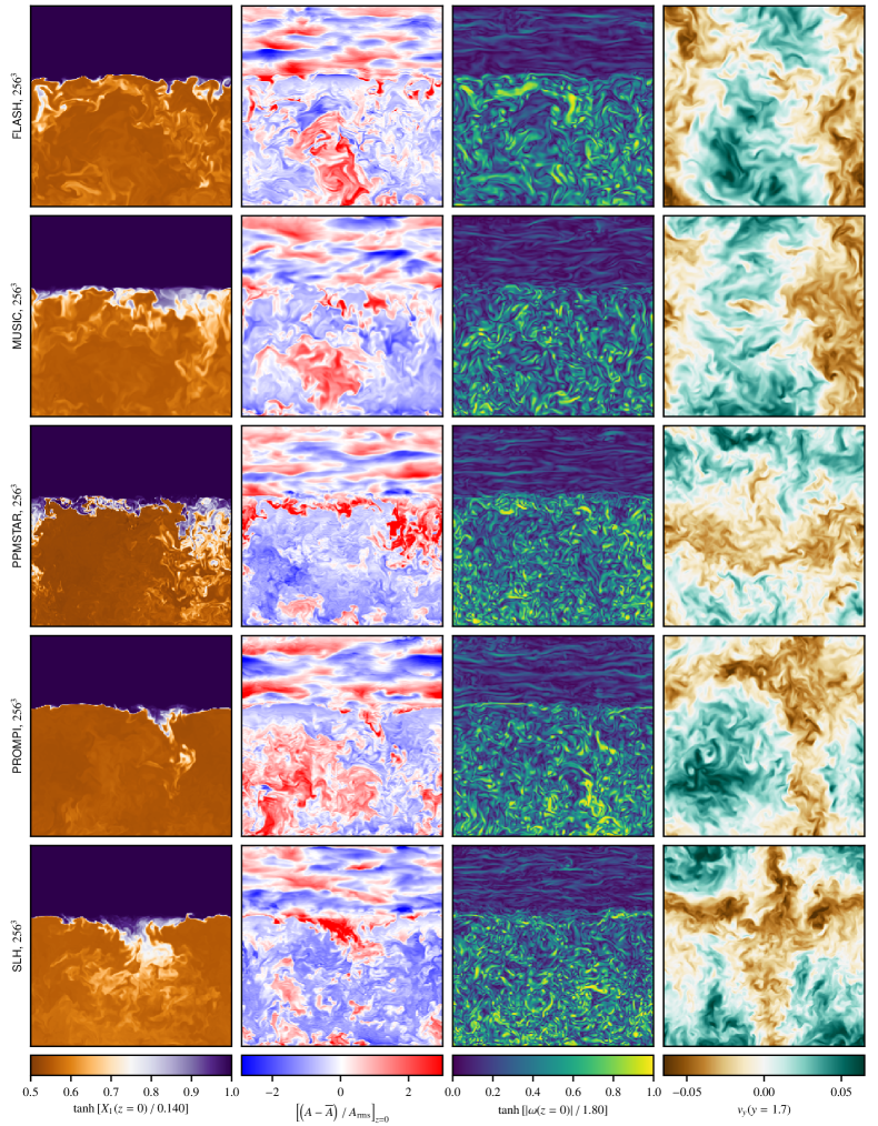
Figure 2: Renderings of the flow field at $t\,{=}\,1000$. The variables shown (from left to right) are the mass fraction $X_{1}$, relative entropy fluctuations $(A-\overline{A})/A_{\mathrm{rms}}$, magnitude of vorticity $|\omega|$, and the vertical component of velocity $v_{y}$. The first three variables correspond to slices through the simulations box in the $z\,{=}\,0$ plane and the last one in the $y\,{=}\,1.7$ plane. The non-linear scaling of $X_{1}$ and $|\omega|$ and the normalisation of entropy fluctuations by their horizontal rms spread $A_{\mathrm{rms}}$ (see the colour bars) are introduced for visualisation purposes.

Owing to the well-resolved initial perturbation, the initial growth of convection proceeds at the same rate in all of the codes considered (see Fig. 3 and Sect. 3.1). As the animations available on Zenodo show, a substantial amount of small-scale structure appears in the large-scale hot bubbles during their initial rise from the heating layer towards the top of the convective layer. They deform the convective-stable interface significantly when they impact it at $t\,{\approx}\,60$, generating the first upward-propagating internal gravity waves (IGW). The stable nature of the upper layer forces the convective upflows to decelerate and, ultimately, reverse. As this happens, the flows drag some of the $\mu_{1}$ fluid into the convective layer, starting the process of mass entrainment, see Fig. 2. The flow keeps accelerating during the first few convective timescales $\tau_{\mathrm{conv}}=80$ (see Eq. 16) and we conservatively define the end of this initial transient to be $t_{0}=500\approx 6\,\tau_{\mathrm{conv}}$. We focus our analysis on the remaining $1500$ time units (${\approx}19\,\tau_{\mathrm{conv}}$) of steady convection accompanied with continuous increase in the convective layer’s mass due to mass entrainment. In the following subsections, we present different aspects of the simulations and compare their evolution in the five codes in detail.

3.1 Velocity field

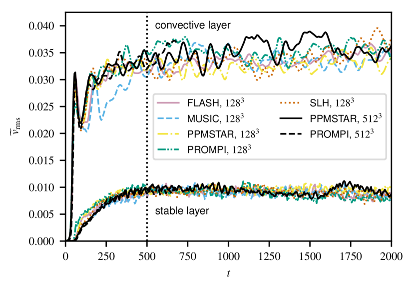
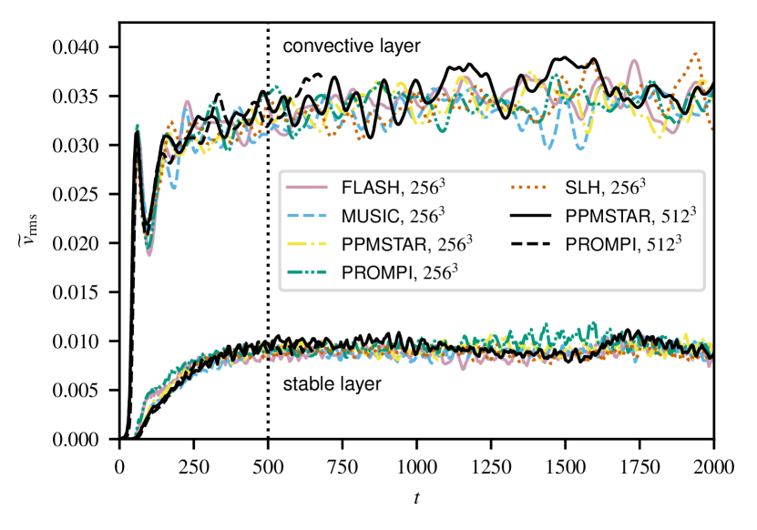
Figure 3: Time evolution of the mass-weighted average rms velocity fluctuations in the convection zone ($y<y_{\mathrm{ub}}(t)-0.1$, upper set of curves) and in the stable layer ($y>y_{\mathrm{ub}}(t)+0.1$, lower set of curves). The location $y_{\mathrm{ub}}(t)$ of the convective boundary is tracked in time as shown in Fig. 9. The dotted vertical line marks the end of the initial transient excluded from the analysis.

We first compare the simulations in terms of horizontally averaged rms velocity fluctuations

$$\widetilde{v}_{\mathrm{rms}}(y)=\left(\widetilde{\sigma}_{v,x}^{\,2}+\widetilde{\sigma}_{v,y}^{\,2}+\widetilde{\sigma}_{v,z}^{\,2}\right)^{\frac{1}{2}},$$ (15)

where $\widetilde{\sigma}_{v,x}$, $\widetilde{\sigma}_{v,y}$, and $\widetilde{\sigma}_{v,z}$ are standard deviations of the three components of the velocity vector. We further average the velocity profiles over the convective and stable layer to obtain (mass-weighted) bulk measures of typical velocity fluctuations in the two layers. Because a substantial amount of mass gets entrained into the convective layer during the simulations, we track the vertical coordinate $y_{\mathrm{ub}}$ of the upper boundary of the convective layer in time as described in Sect. 3.2. We compute the averages in the regions with $y<y_{\mathrm{ub}}(t)-0.1$ (convective layer) and $y>y_{\mathrm{ub}}(t)+0.1$ (stable layer). The offsets of $0.1$ length units are used to exclude the transition zone.

The time evolution of the rms velocity fluctuations in the convective and stable layer is shown in Fig. 3. During the initial transient ($t<t_{0}=500$), the rms velocity in the convective layer increases until it has saturated at a mean value of ${\approx}\,0.034$. Because the speed of sound is approximately $0.8$ in the middle of the convective layer, the typical Mach number is ${\approx}\,0.04$. The flow speed is statistically the same in all of our simulations. This means that even in the $128^{3}$ simulations the convection is a fully developed turbulent flow, in which kinetic energy is dissipated at a rate independent of the code-dependent numerical viscosity close to the grid scale. The $3\sigma$ fluctuations around the mean value of $\widetilde{v}_{\mathrm{rms}}$ range from $11\%$ to $19\%$ with a median value of $13\%$. The $512^{3}$ PPMSTAR run contains two high-velocity episodes in the time intervals $1090\,{\lesssim}\,t\,{\lesssim}\,1250$ and $1440\,{\lesssim}\,t\,{\lesssim}\,1620$, both ${\approx}\,2\tau_{\mathrm{conv}}$ long, during which the bulk convective velocity increases by up to ${\approx}\,15\%$ as compared with the $128^{3}$ and $256^{3}$ runs. These episodes are likely of statistical origin, although we would need an ensemble of $512^{3}$ runs to confirm this hypothesis. When all of the simulations are considered, there is some weak evidence for a slight systematic increase in velocity in the interval $500<t<2000$ with a median value of $4\%$. However, run-to-run values range from $-1\%$ to $15\%$ and seem to be dominated by statistical variation, so we do not subtract the linear trend when computing the magnitude of fluctuations.

The rms velocity in the stable layer initially increases slowly as IGW generated at the convective-stable interface propagate through the stable layer. To understand the slow vertical propagation of the waves, we refer to the 2D renderings of entropy fluctuations in Fig. 2. The renderings show a number of wavefronts spanning almost the full width of the computational domain and inclined at angles of $5^{\circ}\lesssim\vartheta\lesssim 15^{\circ}$ with respect to the horizontal, ignoring projection effects. The Brunt-Väisälä frequency $N_{\mathrm{BV}}$ does not change much across the stable layer and its typical value is $N_{\mathrm{BV}}=0.42$ at $t=0$. Using linear theory of IGW (see e.g. Sutherland, 2010), we estimate that such long waves have periods in the range $2\tau_{\mathrm{conv}}\gtrsim P_{\mathrm{IGW}}\gtrsim 0.7\tau_{\mathrm{conv}}$. The magnitude of the vertical component of their group velocity is $0.001\lesssim v_{y,\mathrm{IGW}}\lesssim 0.01$, implying that it takes the waves between ${\approx}100$ and ${\approx}1000$ time units to propagate from the initial convective-stable interface at $y=2$ to the upper boundary condition at $y=3$. Projection effects, which decrease the apparent angle $\vartheta$ in the 2D slices, make this estimate slightly biased towards longer timescales. Nevertheless, Fig. 3 shows that the final velocity amplitude of ${\approx}\,0.009$ in the stable layer is reached by $t\,{=}\,t_{0}\,{=}\,500$ in all of our simulations. This observation, combined with the estimate above suggests that there cannot be strong resonant wave amplification caused by many wave reflections between the upper boundary of the simulation box and the convective-stable interface because that would cause the rms velocity to increase on much longer timescales. Finally, the fact that the rms velocity reaches the same value on grids ranging from $128^{3}$ to $512^{3}$ implies that the dominant wave patterns are well resolved even on the coarsest grid. This conclusion is further supported by kinetic-energy spectra, which we discuss at the end of this section.

We define the convective turnover timescale to be

$$\tau_{\mathrm{conv}}=\frac{2\langle\Delta y_{\mathrm{cl}}\rangle}{\langle\widetilde{v}_{\mathrm{rms}}\rangle}=80,$$ (16)

where $\langle\widetilde{v}_{\mathrm{rms}}\rangle=0.034$ is the above-mentioned characteristic convective velocity and

$$\langle\Delta y_{\mathrm{cl}}\rangle=\langle y_{\mathrm{ub}}\rangle-y_{\mathrm{bot}}=1.36$$ (17)

is the average depth of the convective layer, that is the distance between the layer’s bottom at $y_{\mathrm{bot}}=1$ and the vertical coordinate $y_{\mathrm{ub}}$ of the upper convective boundary averaged in the time interval $500\leq t\leq 2000$, see Fig. 9 and Sect. 3.2 for details. To show how well this timescale describes variability in the global convective velocity field, we compute the autocorrelation function

$$R(\Delta t)=\frac{\int_{t_{0}}^{t_{\mathrm{end}}}\widetilde{v}_{\mathrm{rms}}^{\,*}(t)\ \widetilde{v}_{\mathrm{rms}}^{\,*}(t+\Delta t)\,\mathrm{d}t}{\int_{t_{0}}^{t_{\mathrm{end}}}\widetilde{v}_{\mathrm{rms}}^{\,*}(t)^{2}\,\mathrm{d}t},$$ (18)

where $\Delta t$ is a time shift and $\widetilde{v}_{\mathrm{rms}}^{\,*}(t)$ is constructed from the bulk convective velocity $\widetilde{v}_{\mathrm{rms}}(t)$ as follows: (1) the initial transient ($t<t_{0}$) is discarded, (2) the best-fit linear trend is subtracted to suppress spurious correlations caused by any slight systematic changes in $\widetilde{v}_{\mathrm{rms}}(t)$ on long timescales, and (3) the resulting time series is made periodic by appending to it a time-reversed version of itself. Figure 4 shows that $R(\Delta t)$ reaches high values for $\Delta t\lesssim 0.5\tau_{\mathrm{conv}}$, implying that the time series is strongly correlated on such short timescales. However, $R(\Delta t)$ decreases steeply and, although the function’s first zero crossing occurs at $\Delta t<\tau_{\mathrm{conv}}$ in some runs and at $\Delta t>\tau_{\mathrm{conv}}$ in others due to stochasticity, $\Delta t\approx\tau_{\mathrm{conv}}$ is generally a good estimate of the temporal spacing between different, largely independent, flow realisations.

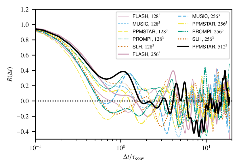
Figure 4: Autocorrelation function $R(\Delta t)$ of the convective velocity as a function of the time shift $\Delta t$ in units of the convective turnover timescale $\tau_{\mathrm{conv}}$. See Eq. 18 and the associated text in detail.

Figure 5 shows time-averaged profiles of rms vertical and horizontal velocity fluctuations,

$$\widetilde{v}_{y,\mathrm{rms}}(y) =\widetilde{\sigma}_{v,y},$$ (19)

$$\widetilde{v}_{xz,\mathrm{rms}}(y) =\left(\widetilde{\sigma}_{v,x}^{\,2}+\widetilde{\sigma}_{v,z}^{\,2}\right)^{\frac{1}{2}}.$$ (20)

The vertical fluctuations $\langle\widetilde{v}_{y,\mathrm{rms}}\rangle$ reach a broad maximum close to the middle of the convective layer. They vanish at the bottom of the simulations box as required by the wall boundary conditions but they also drop by as much as a factor of four at the transition to the stable layer. The velocity field is dominated by the horizontal component $\langle\widetilde{v}_{\mathrm{xz,rms}}\rangle$ close to the boundaries of the convective layer, where the flow has to turn around, and in the stable layer filled with internal gravity waves. The velocity profiles are nearly constant in the bulk of the stable layer with $\langle\widetilde{v}_{\mathrm{xz,rms}}\rangle\,/\,\langle\widetilde{v}_{y,\mathrm{rms}}\rangle\,{\approx}\,2$ and only a mild increase in velocity towards lower densities. There is another drop in $\langle\widetilde{v}_{y,\mathrm{rms}}\rangle$ at $y\gtrsim 2.9$ as gravity is turned off (Eq. 2), removing the waves’ restoring force, and the upper wall boundary condition forces $\langle\widetilde{v}_{y,\mathrm{rms}}\rangle$ to vanish at $y=3$.

It is clear from Fig. 5 that all five codes produce similar time-averaged velocity profiles. However, we have to take the stochastic character of turbulent convection into account to see whether the remaining differences are significant. Instead of running ensembles of simulations with randomised initial conditions, which would be rather expensive, we obtain the $\pm 3\sigma$ statistical-variation bands shown in Fig. 5 as follows. The central curve of each band corresponds to the arithmetic average of all velocity profiles available on a given computational grid. We also compute the standard deviations of each time series in the averaging time window at each height $y$ and we average the standard deviation profiles over the same set of runs to obtain one standard deviation profile $\sigma_{0}(y)$. The profile $\sigma_{0}(y)$ is our best estimate of the statistical variation to be expected in any of the runs, provided that they are statistically similar, and it does not depend on any small systematic differences between the velocity amplitudes predicted by different codes. Obviously, the statistical variation associated with the time averages should decrease as the length of the averaging interval is increased. We show above that there is approximately one independent realisation of the convective flow per turnover timescale $\tau_{\mathrm{conv}}$, so we estimate the statistical variation associated with the time-averaged profiles to be $\sigma(y)=\sigma_{0}(y)/\sqrt{N_{\mathrm{conv}}}$, where $N_{\mathrm{conv}}$ is the length of the averaging time window in units of $\tau_{\mathrm{conv}}$.

However, we must keep in mind that $\sigma(y)$ is just an estimate, which involves both statistical and systematic uncertainties. It depends on our assumption that independent flow realisations are spaced by $\tau_{\mathrm{conv}}$ in time. Figure 4 shows that the spacing could also be estimated to be $0.5\tau_{\mathrm{conv}}$ or $2\tau_{\mathrm{conv}}$, depending on which set of runs we use and on the very definition of ‘decorrelation’. Moreover, the autocorrelation function $R(\Delta t)$ is based on the time evolution of the bulk convective velocity. Different parts of the simulation domain may have different characteristic timescales and our use of $\tau_{\mathrm{conv}}$ everywhere may bias the estimate of $\sigma(y)$. We should thus use the statistical-variation bands as a general guideline in quantifying differences between simulations but this simple approach does not allow us to calculate the probability that a deviation of a given magnitude is observed under the null hypothesis that the codes do not differ.

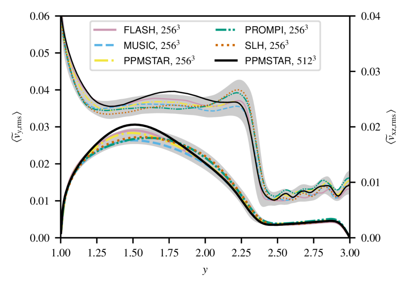
Figure 5: Vertical profiles of the rms velocity components $\langle\widetilde{v}_{y,\mathrm{rms}}\rangle$ (thick lines) and $\langle\widetilde{v}_{\mathrm{xz,rms}}\rangle$ (thin lines) in the vertical and horizontal directions, respectively, averaged in a time interval $\tau_{\mathrm{av}}=6\tau_{\mathrm{conv}}=480$ wide and centred on time $1250$. The two velocity axes in each plot have different scales to avoid the curves’ overlapping. The grey bands give an estimate of $\pm 3\sigma$ statistical variation in the averages due to stochasticity, see Sect. 3.1 for details.

Figure 5 shows that the profiles of both velocity components in the $128^{3}$ and $256^{3}$ runs fall within or close to the respective estimated $\pm 3\sigma$ statistical-variation bands. This means that the small code-to-code differences are dominated by stochasticity. The bands of both the $128^{3}$ and $256^{3}$ runs are slightly below the velocity curves of the $512^{3}$ PPMSTAR run in the convective layer, suggesting that velocity profiles may not be fully converged on the $256^{3}$ grid. However, the time-averaging window overlaps with the two above-mentioned episodes visible in Fig. 3, during each of which the $512^{3}$ PPMSTAR run reaches above-average bulk velocities for as much as ${\approx}\,2\tau_{\mathrm{conv}}$. Given the uncertainty in determining the width of the statistical-variation bands and the fact that we only have a single full-length $512^{3}$ run, we do not find the tension between the velocity profiles significant.

The arguments leading to our scaling the width of the statistical-variation bands with $1/\sqrt{N_{\mathrm{conv}}}$ do not apply to the stable layer directly because the response timescale of the stable layer is longer than $\tau_{\mathrm{conv}}$ (see above). Nevertheless, Fig. 5 shows that the statistical-variation bands describe the range of code-to-code variation rather well. The velocity profiles of all $128^{3}$ and $256^{3}$ runs closely match that of the $512^{3}$ PPMSTAR run both in shape and amplitude, which further supports our conclusion that the dominant wave patterns are essentially converged already on the $128^{3}$ grid.

The renderings of the vertical component of velocity $v_{y}$ in the horizontal midplane of the convective layer presented in Fig. 2 show that the convective flow is dominated by the largest possible scales with wavelengths equal to the width of the computational box. This corresponds to convective cells with an aspect ratio of about unity early in the simulations, which later become slightly elongated in the vertical direction as the convective boundary moves upwards. The cells are turbulent on smaller scales with large amounts of small-scale vorticity $\omega$, also shown in Fig. 2 and in the animations available on Zenodo. We compute spatial Fourier spectra of the velocity vector,

$$\bm{\Psi}_{jl} =\frac{1}{N_{x}N_{z}}\sum_{m=0}^{N_{x}-1}\sum_{n=0}^{N_{z}-1}\bm{v}_{mn}\exp\left\{-2\pi i\left(\frac{mj}{N_{x}}+\frac{nl}{N_{z}}\right)\right\},$$ (21)

$$j =0,\dots,N_{x}-1,$$ (22)

$$l =0,\dots,N_{z}-1,$$ (23)

where $N_{x}$ and $N_{z}$ are the total numbers of computational cells along the $x$ and $z$ axes, respectively. The velocity array $\bm{v}_{mn}$ corresponds to a horizontal slice through the simulation box at $y=1.7$, which is close to the midplane of the convective layer at $t\approx 1250$. We compare the kinetic energy per unit mass $\frac{1}{2}||\,|\bm{\Psi}|\,||^{2}$ binned over all wavenumbers $k=\left(k_{x}^{2}+k_{z}^{2}\right)^{1/2}$, where

$$k_{x}$$ (24)

(25)

kz&={l,0≤l<Nz2-1, -Nz+l,Nz2≤l<Nz.

These expressions hold for even values of $N_{x}$ and $N_{z}$, which is the case for all of our computational grids. Figure 6 shows the spectra averaged in the whole time interval of analysis ($500\leq t\leq 2000$). Although the turbulence is anisotropic at small wavenumbers (large scales), it looks close to being isotropic at the larger wavenumbers (smaller scales) that we see in the renderings of vorticity in Fig. 2. All of the codes converge to the same kinetic energy spectrum upon grid refinement, which is consistent with Kolmogorov’s $-\frac{5}{3}$ law. Although we only use the $k_{x}$ and $k_{z}$ components of the wavenumber vector for simplicity, the kinetic-energy spectrum of isotropic turbulence should have the same slope along all three axes of the wavenumber space in the inertial range. If this was not the case there would be more power along one or two of the axes on small scales in conflict with the assumption of isotropy.

The $512^{3}$ PPMSTAR run illustrates that a rather fine grid is needed to obtain a wide and well-converged inertial range. This is due to the well-known bottleneck effect – a power excess observed in numerical simulations of turbulence between the inertial and dissipation ranges (e.g. Falkovich, 1994; Sytine et al., 2000; Dobler et al., 2003). All of our spectra have similar shapes even in the dissipation range, although they diverge with increasing $k$ and they reach a spread of as much as a factor of $10$ at the Nyquist frequency. The spectrum in the dissipation range depends on the behaviour of the numerical scheme close to the grid scale. However, this dependence is largely irrelevant thanks to the fact that the dissipation rate becomes independent of the magnitude of small-scale viscosity (be it of physical or numerical origin) in turbulent flows as long as the viscosity is small enough.

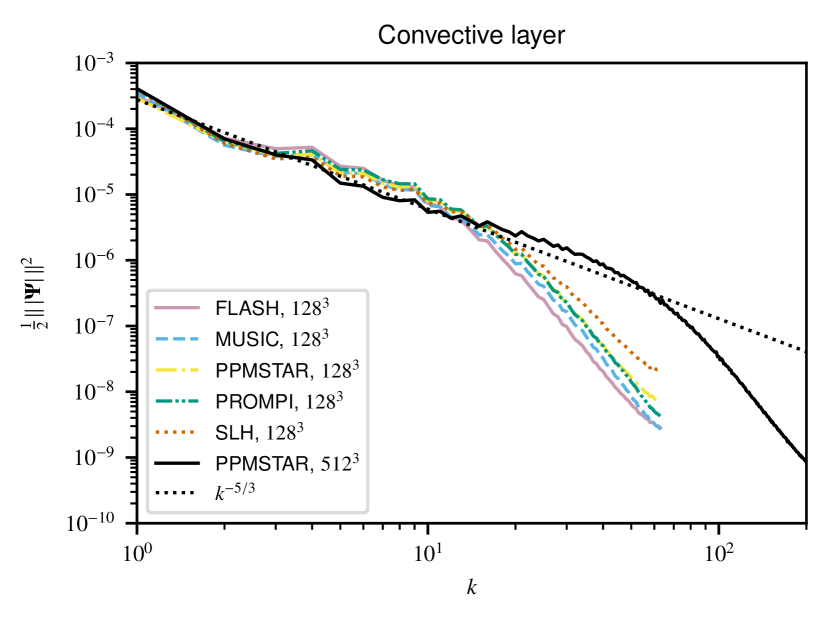
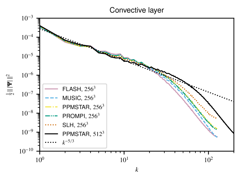
Figure 6: Spectra of kinetic energy as functions of the wavenumber $k$ in a horizontal slice through the convective layer at $y=1.7$. The spectra have been averaged over the whole analysis time interval ($500\leq t\leq 2000$, approximately $19\,\tau_{\mathrm{conv}}$). The Kolmogorov scaling $k^{-5/3}$ is shown for comparison.

We use the same procedure to characterise the spatial spectra at $y=2.7$ in the stable layer, see Fig. 7. These spectra are also dominated by the largest scales, which can also be seen in the 2D renderings of entropy fluctuations in Fig. 2. Although we do not have any analytic prediction of the wave spectrum, all five codes predict essentially the same spectrum at $k\lesssim 5$ on the $128^{3}$ grid and at $k\lesssim 10$ on the $256^{3}$ grid, respectively. This corresponds to horizontal wavelengths $\gtrsim 26$ computational cells in both cases. Although this seems to be a large number, the actual challenge is to resolve the vertical wavelength of the IGW, which is several times shorter as the waves are nearly horizontal. The most extreme of these are revealed in the 2D renderings of vorticity $\omega$ in Fig. 2, which put more emphasis on shorter vertical wavelengths as compared with the renderings of entropy fluctuations.

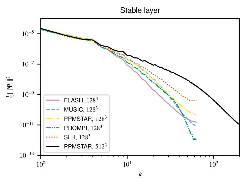
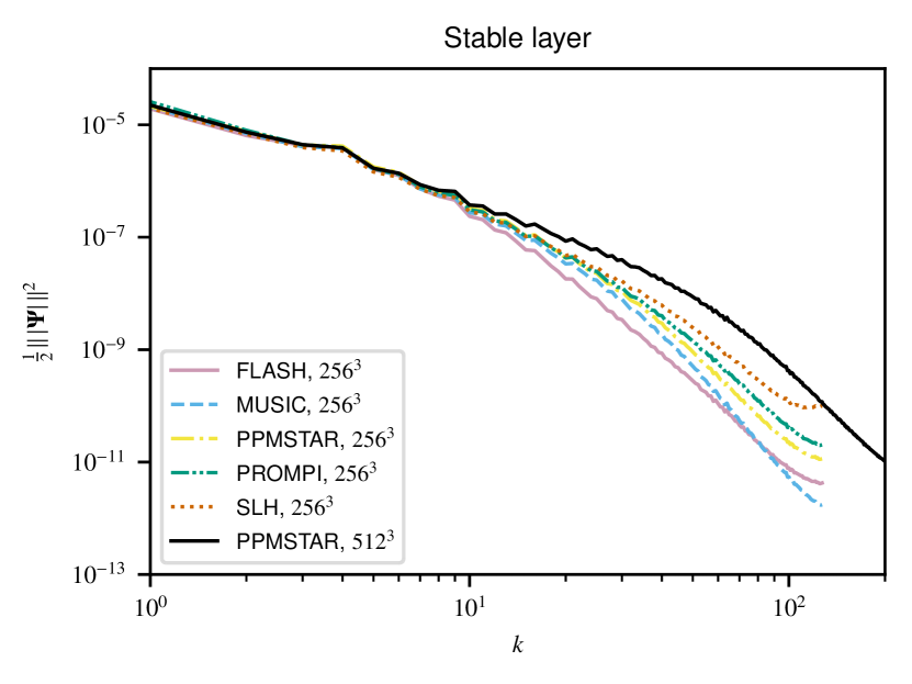
Figure 7: Spectra of kinetic energy as functions of the wavenumber $k$ in a horizontal slice through the stable layer at $y=2.7$. The spectra have been averaged over the whole analysis time interval ($500\leq t\leq 2000$, approximately $19\,\tau_{\mathrm{conv}}$).

3.2 Convective boundary and mass entrainment

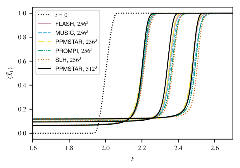
Figure 8: Mass entrainment process visualised using vertical profiles of the mass fraction of the $\mu_{1}$ fluid. Only the uppermost parts of the convective layer and part of the stable layer are shown. The dotted line shows the initial condition and the remaining three sets of lines correspond to averages over time windows $\tau_{\mathrm{av}}\,=\,2\,\tau_{\mathrm{conv}}\,=\,160$ wide and centred on times of (from left to right) $580$, $1250$, and $1920$.

When upflows reach the upper boundary of the convective layer, they stir and entrain some of the $\mu_{1}$ fluid in the transition zone and carry it down into the convective layer as they turn around. The distribution of this fluid’s mass fraction $X_{1}$, shown in Fig. 2, provides a good visual representation of the entrainment process. The process also involves the mixing of entropy, which flattens the entropy gradient in the transition zone and makes the convective layer grow. The gradual growth can be seen in the profiles of the mass fraction $X_{1}$ shown in Fig. 8.

We define the vertical coordinate $y_{\mathrm{ub}}$ of the convective boundary to be where $\partial_{y}\widetilde{X}_{1}$ reaches its global maximum. Discretisation noise is reduced by fitting a parabola to the three data points closest to the discrete estimate of the maximum’s vertical coordinate. Figure 9 shows that the $128^{3}$ runs diverge in $y_{\mathrm{ub}}(t)$ slightly with FLASH and PROMPI predicting the slowest and fastest boundary motion, respectively. However, the relative difference in the distance travelled by the end of the simulations, $\Delta y_{\mathrm{ub}}(t_{\mathrm{end}})=y_{\mathrm{ub}}(t_{\mathrm{end}})-y_{\mathrm{ub}}(0)$, is only ${\approx}14\%$ between these two extremes. The spread is reduced by another factor of ${\approx}\,3$ on the $256^{3}$ grid, on which all five codes agree on $\Delta y_{\mathrm{ub}}(t_{\mathrm{end}})$ within $5\%$. Moreover, the $y_{\mathrm{ub}}(t)$ curves derived from the $256^{3}$ runs closely track those from the $512^{3}$ PROMPI and PPMSTAR runs.

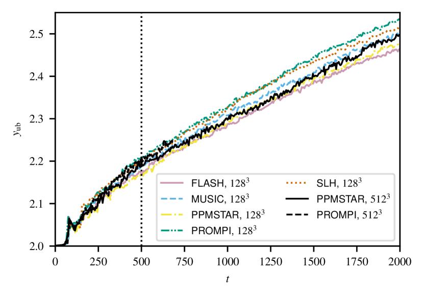
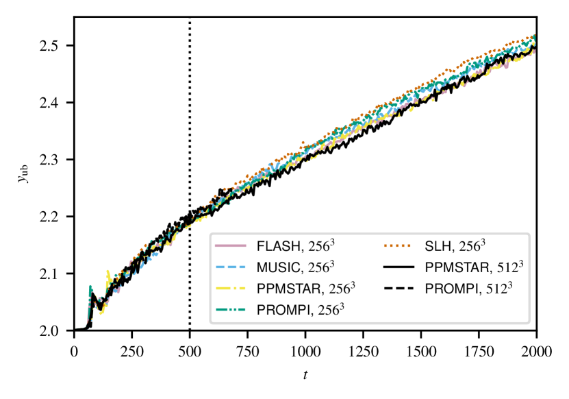
Figure 9: Time evolution of the $y$ coordinate of the upper boundary of the convection zone as determined from 1D averages. The dotted vertical line marks the end of the initial transient excluded from the analysis.

We characterise the thickness of the convective boundary using the scale height

$$H_{\mathrm{ub}}=\left[\widetilde{X}_{1}\left(\frac{\partial\widetilde{X}_{1}}{\partial y}\right)^{-1}\right]_{y=y_{\mathrm{ub}}}.$$ (26)

Because this quantity is highly variable on short timescales, we smooth the time series using a top-hat filter $\tau_{\mathrm{av}}\,{=}\,\tau_{\mathrm{conv}}\,{=}\,80$ wide and show the result in Fig. 10. In all five codes, the boundary is up to $50\%$ thicker on the $128^{3}$ grid than on the $256^{3}$ grid. However, differences between the $256^{3}$ and $512^{3}$ runs are substantially smaller, suggesting that $H_{\mathrm{ub}}$ is close to being converged on the $256^{3}$ grid at a value of ${\approx}\,0.04$. The converged value is close to the initial value $H_{\mathrm{ub}}(t\,{=}\,0)=0.0404$. This fact, however, is purely coincidental. At $t\,{=}\,0$, $H_{\mathrm{ub}}$ characterises the steepness of the 1D transition zone as we define it. Once convection has started, $H_{\mathrm{ub}}$ is a product of spatial averaging along a 3D convective boundary that is as sharp as the numerical scheme allows at some places but much wider at other places, see Fig. 2. The converged thickness $H_{\mathrm{ub}}\,{\approx}\,0.04$ corresponds to $10$ computational cells on the $512^{3}$ grid, although the PPB advection method implemented in PPMSTAR can preserve gradients spanning only about two computational cells (Woodward et al., 2015). This suggests that the 3D deformation of the boundary dominates the thickness of the spatially averaged boundary. However, it is much more challenging for the codes to resolve the physical thickness of the boundary on the $256^{3}$ and $128^{3}$ grids, on which $0.04$ units of length correspond to only about $5$ and $2.5$ computational cells, respectively.

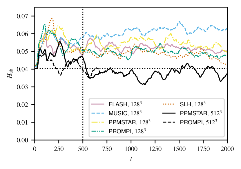
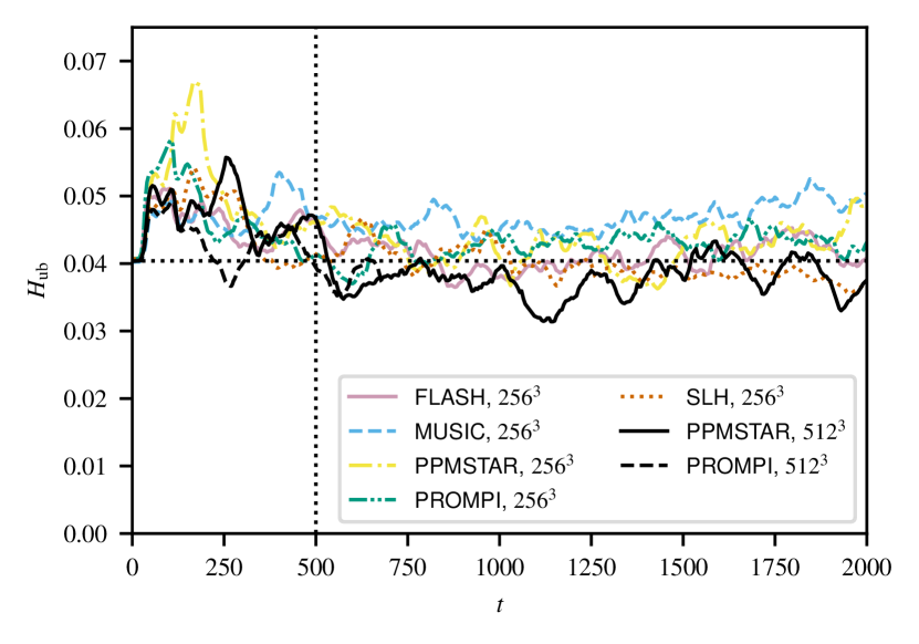
Figure 10: Time evolution of the thickness $H_{\mathrm{ub}}$ (Eq. 26) of the upper convective boundary. The time series have been smoothed using convolution with a top-hat kernel $\tau_{\mathrm{av}}\,=\,\tau_{\mathrm{conv}}\,=\,80$ wide. The dotted vertical line marks the end of the initial transient excluded from the analysis. The dotted horizontal line shows $H_{\mathrm{ub}}(t\,{=}\,0)=0.0404$ for comparison.

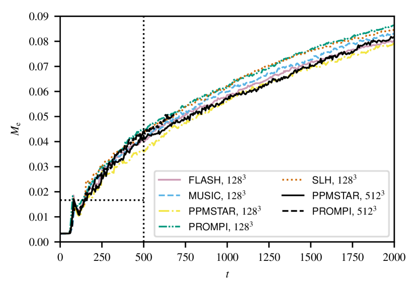
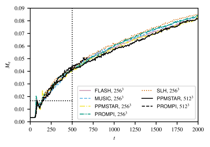
Figure 11: Mass per unit horizontal area of the $\mu_{1}$ fluid entrained into the convective layer as a function of time. The dotted vertical line marks the end of the initial transient excluded from the analysis. The dotted horizontal line shows the amount of the $\mu_{1}$ fluid contained in the initial transition zone between the convective and stable layer.

The total amount of the $\mu_{1}$ fluid entrained by time $t$ is

$$M_{\mathrm{e}}(t)=\int_{1}^{y_{\mathrm{ub}}(t)}\widetilde{X}_{1}(y,t)\,\overline{\rho}(y,t)\,\mathrm{d}y$$ (27)

per unit of horizontal surface area and is shown in Fig. 11. This entrainment metric differs slightly from $y_{\mathrm{ub}}(t)$ because of the density stratification. The agreement between the codes’ predictions is slightly better as compared with the $y_{\mathrm{ub}}(t)$ metric and the $128^{3}$ and $256^{3}$ simulations agree within $9\%$ and $4\%$, respectively, on the total amount of the $\mu_{1}$ fluid entrained by the end of the simulations. All of the initial transition layer is entrained early on during the initial transient as indicated in Fig. 11.

It is also clear from Fig. 11 that the mass entrainment rate $\dot{M}_{\mathrm{e}}(t)$ is relatively high early on and slowly decreases throughout the simulation time. We compute $\dot{M}_{\mathrm{e}}(t)$ using second-order central differences. The differencing greatly amplifies noise, which we suppress using convolution with a centred top-hat kernel $\tau_{\mathrm{av}}\,{=}\,3\tau_{\mathrm{conv}}\,{=}\,240$ wide. The mass entrainment rates, shown in Fig. 12, agree between all of the codes within their statistical fluctuations already on the $128^{3}$ grid and they remain unchanged as the grid is refined up to $512^{3}$. However, $\dot{M}_{\mathrm{e}}(t)$ varies randomly on timescales as long as several convective turnover timescales, which likely contributes to the small spread in $M_{\mathrm{e}}(t)$ in Fig. 11. The entrainment rate decreases from ${\approx}\,1.0\times 10^{-4}$ at the beginning of the initial transient to ${\approx}\,4.5\times 10^{-5}$ at $t=t_{0}$ and to ${\approx}\,2.0\times 10^{-5}$ at $t=t_{\mathrm{end}}$. Part of the decrease may be attributed to the density at the convective boundary, which decreases from $0.28$ at $t=0$ to $0.15$ at $t=t_{\mathrm{end}}$.

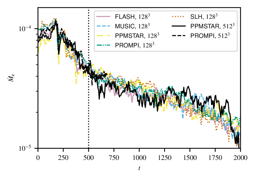
Figure 12: Mass entrainment rates corresponding to the curves shown in Fig. 11. The time series have been smoothed using convolution with a top-hat kernel $\tau_{\mathrm{av}}=3\,\tau_{\mathrm{conv}}=240$ wide. The dotted vertical line marks the end of the initial transient excluded from the analysis.

One may find it surprising that the mass entrainment rates obtained on the coarse $128^{3}$ grid agree so well with one another. Perhaps even more surprisingly, they also agree with the rates obtained in the $512^{3}$ PROMPI and PPMSTAR runs. Convective mass entrainment is usually thought of as a complex process sensitive to small-scale flows and instabilities in the boundary layer. However, Spruit (2015) argues that the mass entrainment rate is set by the amount of energy available to overcome the buoyancy of the fluid being entrained; this was also observed in a laboratory study by Linden (1975). Applying this constraint in models of stars with helium-burning convective cores improves their agreement with both asteroseismology and population studies of globular clusters (Constantino et al., 2017). The entrainment rate is then proportional to the luminosity $L$ driving the convective flow as confirmed by the 3D simulations of Jones et al. (2017) and Andrassy et al. (2020) of oxygen burning in a setup similar to our present test setup. More evidence comes from calibrations of the entrainment law $\dot{M}_{\mathrm{e}}\propto v_{\mathrm{rms}}\,\mathrm{Ri_{B}}^{-n}$, where $v_{\mathrm{rms}}$ is the rms velocity of convection and $\mathrm{Ri_{B}}$ is the bulk Richardson number proportional to $v_{\mathrm{rms}}^{-2}$ for a given convective boundary (for a complete definition, see Meakin & Arnett, 2007). Assuming that $v_{\mathrm{rms}}\,{\propto}\,L^{1/3}$, we have $\dot{M}_{\mathrm{e}}\,{\propto}\,L^{(1+2n)/3}$ and $n\,{=}\,1$ corresponds to $\dot{M}_{\mathrm{e}}\,{\propto}\,L$. Values of $n$ measured in different numerical simulations range from $0.74\pm 0.04$ (Cristini et al., 2019) and $0.74\pm 0.01$ (Horst et al., 2021) through $1.05\pm 0.21$ (Meakin & Arnett, 2007) to $1.32\pm 0.79$ (Higl et al., 2021). If buoyancy is the dominant factor one can expect to obtain a good estimate of the entrainment rate as soon as the largest downflows are reasonably resolved.

Finally, the very fact that we keep increasing the mean entropy of the convective layer by heating it at the bottom contributes to mass entrainment. This process, previously mentioned by Meakin & Arnett (2007), Andrassy et al. (2020), and Horst et al. (2021), can be understood as follows. The convective layer is well mixed and its entropy is essentially constant in space. On the other hand, entropy increases with height in the stable layer (Fig. 1). If the mean entropy of the convective layer increases it becomes higher than that of a thin layer at the very bottom of the stable layer. This thin layer is thus negatively buoyant and it must sink and mix with the convective layer. In our simulations, we compute the rate of change of the mean entropy in the lower $\nicefrac{{2}}{{3}}$ of the convective layer to eliminate any influence of the convective boundary. The value of $\mathrm{d}A/\mathrm{d}t$ reaches $4.7\times 10^{-5}$ by $t\approx 150$ in our $256^{3}$ runs and it remains statistically constant until the end of the simulations. The entrainment rate due to the process described above is $\dot{M}_{\mathrm{e,heating}}=(\mathrm{d}A/\mathrm{d}t)\,/\,(\mathrm{d}A/\mathrm{d}m_{1})$, where $m_{1}$ is the cumulative mass of the $\mu_{1}$ fluid integrated from the bottom of the simulation box upwards. We measure the entropy gradient $\mathrm{d}A/\mathrm{d}m_{1}$ in the initial stratification. Its value is $1.6$ at the top of the initial transition layer between the two fluids and $3.8$ where $m_{1}=M_{\mathrm{e}}(t=t_{\mathrm{end}})\doteq 0.083$ (see Fig. 11). This implies that $\dot{M}_{\mathrm{e,heating}}=2.9\times 10^{-5}$ early on during the initial transient, which is $\approx 30\%$ of the entrainment rate $\dot{M}_{\mathrm{e}}$ measured. This contribution increases to as much as $\approx 60\%$ by the end of the simulations.

3.3 Fluctuations and transport of energy

The rates of convective transport of energy and chemical composition scale with the flow speed and with the magnitude of fluctuations in the flow field. We have already shown that the flow speed is code-independent, see Sect. 3.1. Figure 13 shows that the same holds for the time-averaged relative fluctuations in entropy $\langle\Delta\overline{A}/\overline{A}\rangle$ and in the mass fraction of the $\mu_{1}$ fluid $\langle\Delta\overline{X}_{1}/\overline{X}_{1}\rangle$. The figure includes statistical-variation bands computed as described in Sect. 3.1. The profiles of the fluctuations as produced by all of the five codes fall within or close to the corresponding statistical-variation band. The profiles of $\langle\Delta\overline{A}/\overline{A}\rangle$ agree better on the $256^{3}$ grid in the bulk of the convection zone, although the differences are small already on the $128^{3}$ grid. The slight code-to-code differences in the time-averaged position of the convective boundary (where $\langle\Delta\overline{X}_{1}/\overline{X}_{1}\rangle$ drops) decrease as the mass entrainment rate converges upon grid refinement, see Sect. 3.2.

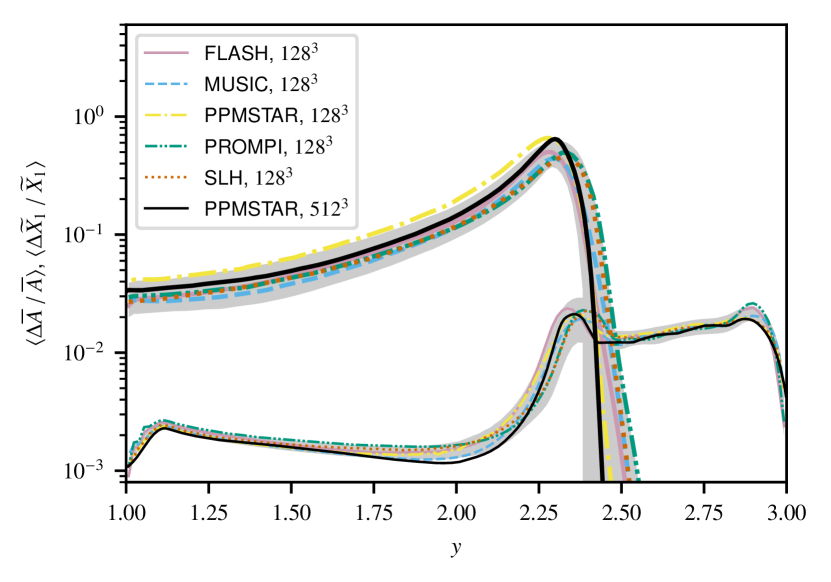
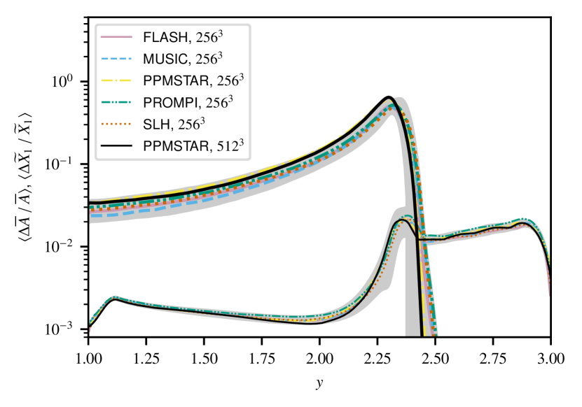
Figure 13: Relative fluctuations in entropy $\overline{A}$ (thin lines) and mass fraction $\widetilde{X}_{1}$ of the $\mu_{1}$ fluid (thick lines) averaged in a time interval $\tau_{\mathrm{av}}=6\,\tau_{\mathrm{conv}}=480$ wide and centred on time $1250$. The grey bands give an estimate of $\pm 3\sigma$ statistical variation in the averages due to stochasticity, see Sect. 3.1 for details.

We define the flux of enthalpy to be the quantity

$$\mathcal{F}_{H}=\overline{Hv_{y}}-\overline{H}\,\widetilde{v}_{y},$$ (28)

where $H$ is enthalpy per unit volume and $v_{y}$ is the vertical component of velocity. The second term in Eq. 28 is included to remove the flux contribution of the thermal expansion and compression of the horizontally averaged stratification. We average the enthalpy flux over all of the simulation time after the initial transient ($500\leq t\leq 2000$), ignoring the upward propagation of the convective boundary and focusing on the bulk of the convective layer instead. The profiles of $\mathcal{F}_{H}(y)$ shown in Fig. 15 agree well within the statistical-variation bands computed as described in Sect. 3.1, although our method seems to overestimate the statistical variation in this quantity as it is significantly larger than the code-to-code differences.

To explain this, we compute the autocorrelation function $R_{\mathcal{F}_{H}}(\Delta t)$ of $\mathcal{F}_{H}(y\,{=}\,1.5)$ using the method described in Sect. 3.1. The shape of $R_{\mathcal{F}_{H}}(\Delta t)$ turns out to be rather different from the autocorrelation function $R(\Delta t)$ of the bulk convective velocity; compare Fig. 14 with Fig. 4. First, the autocorrelation drops to zero on a timescale as short as ${\approx}\,0.3\tau_{\mathrm{conv}}$. This suggests that the width of the statistical variation bands should be reduced by the factor $0.3^{-\frac{1}{2}}=1.8$, see Sect. 3.1. Moreover, all of our runs show some anticorrelation for $0.3\tau_{\mathrm{conv}}\lesssim\Delta t\lesssim\tau_{\mathrm{conv}}$ before the values of $R_{\mathcal{F}_{H}}(\Delta t)$ start to oscillate around zero for longer time shifts. The anticorrelation suppresses fluctuations in long-term time averages. From the physical point of view, the anticorrelation may reflect the fact that changes to the heat flux divergence result in local heating or cooling of the nearly isentropic stratification and the convective instability provides strong negative feedback, quickly driving the flux profile back to its quasi-stationary shape. In light of this, the ${\approx}10\%$ overestimation of $\mathcal{F}_{H}(y)$ in the lower convection zone in the $128^{3}$ PROMPI run may be statistically significant. However, the $256^{3}$ PROMPI run agrees well with other codes run on the same grid as well as with the $512^{3}$ PPMSTAR run. The small differences between the codes as well as the possible feedback mechanism suggest that $\mathcal{F}_{H}$ is a poor indicator of code or simulation quality.

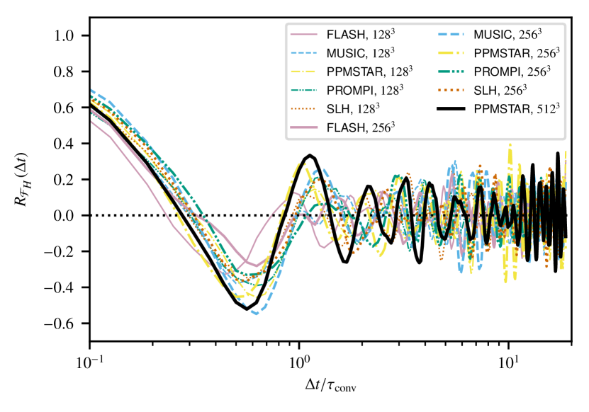
Figure 14: Autocorrelation function $R_{\mathcal{F}_{H}}(\Delta t)$ of $\mathcal{F}_{H}(y\,{=}\,1.5)$ as a function of the time shift $\Delta t$ in units of the convective turnover timescale $\tau_{\mathrm{conv}}$.

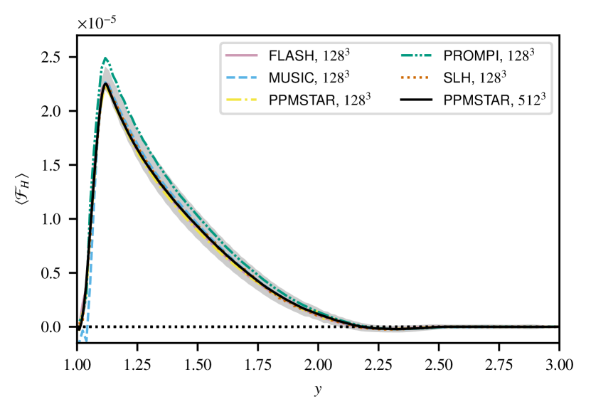
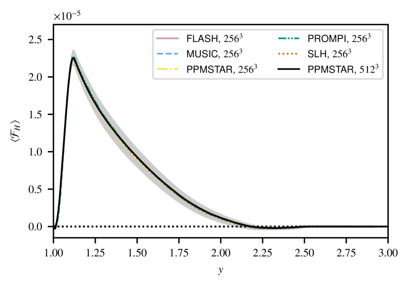
Figure 15: Vertical profiles of the enthalpy flux averaged over the whole analysis time interval ($500\leq t\leq 2000$, approximately $19\,\tau_{\mathrm{conv}}$). The grey bands give an estimate of $\pm 3\sigma$ statistical variation in the averages due to stochasticity, see Sect. 3.1 for details.

The flux of kinetic energy is defined in a way analogous to Eq. 28,

$$\mathcal{F}_{\mathrm{k}}=\frac{1}{2}\left(\overline{\rho\,|\bm{v}|^{2}\,v_{y}}-\overline{\rho\,|\bm{v}|^{2}}\,\widetilde{v}_{y}\right).$$ (29)

Figure 16 shows that the amplitude of $\mathcal{F}_{\mathrm{k}}$ is as much as ${\approx}\,30$ times smaller than that of $\mathcal{F}_{H}$ in our simulations. Stochasticity introduces large statistical variation into the time-averaged profiles of this small quantity. Nevertheless, all of the $128^{3}$ and $256^{3}$ runs agree with each other as well as with the $512^{3}$ PPMSTAR run on the profile of $\mathcal{F}_{\mathrm{k}}$ within the statistical-variation bands included in the figure.

Why is the magnitude of $\mathcal{F}_{\mathrm{k}}$ so much smaller than that of $\mathcal{F}_{H}$? Using a simplified, two-stream model of convection, we show in Appendix B that the magnitude of $\mathcal{F}_{\mathrm{k}}$ depends on the degree of asymmetry between upflows and downflows. We characterise the asymmetry using a downflow filling factor $f_{\mathrm{d}}$ defined to be the relative horizontal area covered by flows with vertical velocity $v_{y}-\widetilde{v}_{y}<0$. In the two-stream model, $\mathcal{F}_{\mathrm{k}}$ vanishes for $f_{\mathrm{d}}=0.5$, that is when there is perfect up-down symmetry. Figure 17 shows that $f_{\mathrm{d}}$ indeed is close to $0.5$ in our simulations. In contrast to $\mathcal{F}_{\mathrm{k}}$, $\mathcal{F}_{H}$ remains a substantial fraction of the total flux even if there is perfect up-down symmetry because convection must transport heat across the convective layer. This explains why the amplitude of $\mathcal{F}_{\mathrm{k}}$ is much smaller than that of $\mathcal{F}_{H}$ in our simulations. The two-stream model also predicts that $\mathcal{F}_{\mathrm{k}}$ is negative (i.e. directed downwards) for $f_{\mathrm{d}}<0.5$ and positive for $f_{\mathrm{d}}>0.5$. We observe the same trend in our simulations: compare Figs. 16 and 17 and see also Fig. 19. The role of $\mathcal{F}_{\mathrm{k}}$ is much more important in strongly stratified, convective stellar envelopes, in which downflows tend to be substantially narrower than upflows and $\mathcal{F}_{\mathrm{k}}$ is large and negative (i.e. directed downwards). Viallet et al. (2013) show this difference directly in their Fig. 13, in which they compare their 3D hydrodynamic models of the convective envelope of a red giant and of an oxygen-burning shell in a massive star. The latter model is rather similar to our test setup and, not surprisingly, they also find that the amplitude of $\mathcal{F}_{\mathrm{k}}$ is ${\approx}\,30$ times smaller than that of $\mathcal{F}_{H}$ in that model (compare their Figs. 13 and 15).

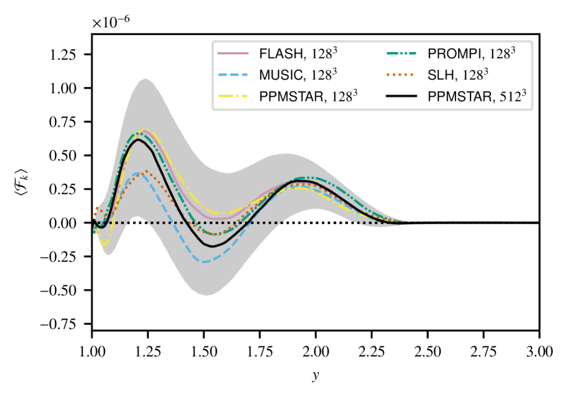
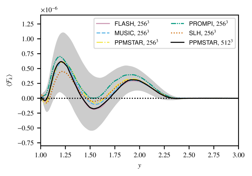
Figure 16: Vertical profiles of the kinetic-energy flux averaged over the whole analysis time interval ($500\leq t\leq 2000$, approximately $19\,\tau_{\mathrm{conv}}$). The grey bands give an estimate of $\pm 3\sigma$ statistical variation in the averages due to stochasticity, see Sect. 3.1 for details.

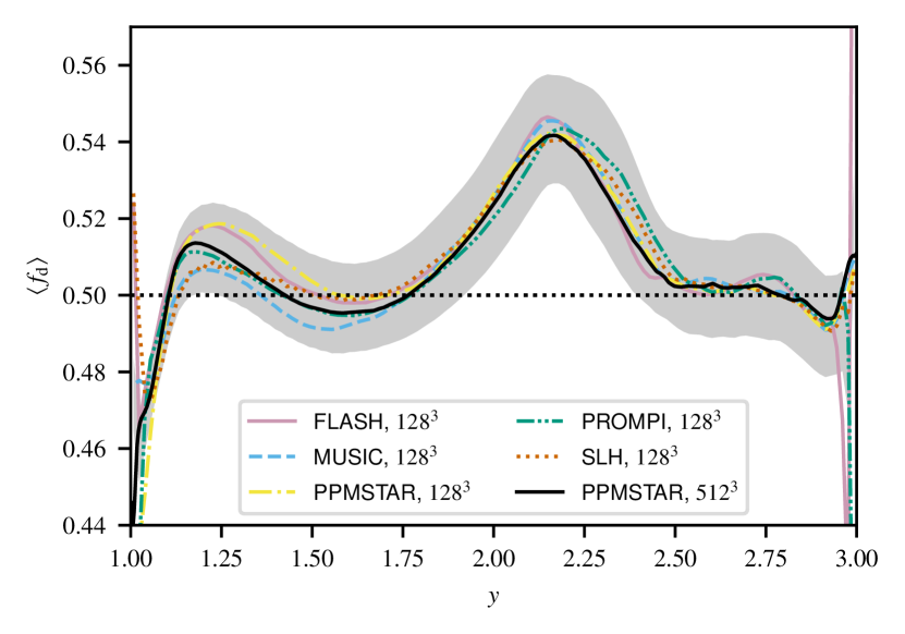
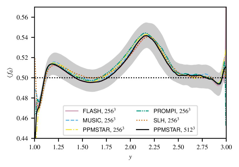
Figure 17: Vertical profiles of the downflow filling factor averaged over the whole analysis time interval ($500\leq t\leq 2000$, approximately $19\,\tau_{\mathrm{conv}}$). The grey bands give an estimate of $\pm 3\sigma$ statistical variation in the averages due to stochasticity, see Sect. 3.1 for details.

4 Summary and conclusions

In this work, we have defined a test problem involving adiabatic turbulent convection and mass entrainment from a stably stratified layer. The problem is directly relevant to current 3D simulation efforts to model convection in stellar interiors. The problem’s physics and geometry are simplified to make it accessible to a wide range of 3D hydrodynamic codes but to retain the crucial processes we are investigating. Because turbulent flows are involved, this test problem is fundamentally different from standard test problems. There is no single solution and the simulations must be compared in a statistical way, taking care not to overinterpret statistical fluctuations as real differences between codes or simulations. We compare simulations computed using the codes FLASH, MUSIC, PPMSTAR, PROMPI, and SLH, which we run for $25$ convective turnover timescales to gather as much statistics as possible.

All of the simulations, computed on Cartesian grids ranging from $128^{3}$ through $256^{3}$ to $512^{3}$ cells, show a turbulent convective layer dominated by large-scale flows with an rms Mach number of ${\approx}\,0.04$. Upflows turning around at the upper convective boundary entrain mass from the bottom of the overlying stable layer and pull it into the convective layer. They also generate internal gravity waves, which are present throughout the stable layer. The bulk rms velocities as well as time- and space-averaged velocity profiles in both the convective and stable layer are statistically the same in all five codes even on the coarse $128^{3}$ grid. They also agree with the profiles obtained on finer grids, although the $512^{3}$ PPMSTAR run deviates slightly because of two long episodes of increased velocity, likely of statistical origin. All of the codes converge to the same kinetic energy spectrum upon grid refinement, which is consistent with Kolmogorov’s $-\frac{5}{3}$ scaling. The five codes slightly differ in their dissipation rates close to the grid scale, which is reflected in slight differences in the shape of the kinetic energy spectrum in the dissipation range. The codes also give essentially the same spectrum in the stable layer for horizontal wavelengths $\gtrsim 26$ computational cells.

The convective boundary is somewhat under-resolved on the $128^{3}$ grid, being as much as ${\approx}\,50\%$ thicker than its converged thickness value as determined by the $256^{3}$ and $512^{3}$ runs. Nevertheless, the simulations agree on the total amount of mass entrained by the simulations’ end within $9\%$ already on the $128^{3}$ grid. This improves to $4\%$ on the $256^{3}$ grid and the remaining spread seems to be dominated by stochasticity. The rapid convergence of the mass entrainment rate upon grid refinement is compatible with the idea of Spruit (2015) that the rate is set by the global energetics of the whole process as opposed to details of the small-scale instabilities occurring in the boundary layer. We also show that approximately $30$ to $60$ per cent of the entrainment rate can be attributed to a process in which mass entrainment is caused by the constant heating of the convective layer and the subsequent increase in its mean entropy.

Finally, all of the codes statistically agree on the time-averaged profiles of fluctuations in composition and entropy and on the profiles of the enthalpy- and kinetic-energy fluxes. This agreement is somewhat better on the $256^{3}$ grid as compared to the $128^{3}$ one. We give likely reasons for the rapid convergence of the time-averaged enthalpy flux, which makes it a rather poor indicator of code or simulation quality. The flux of kinetic energy is ${\approx}\,30$ times smaller than the flux of enthalpy in our test problem. We explain this disparity using a toy model showing that the flux of kinetic energy is very small indeed when the horizontal areas covered by upflows and downflows are close to being the same as observed in our simulations.

All in all, we find excellent code-to-code agreement on a rather complex turbulent-flow problem. The numerical schemes implemented in these codes differ in many aspects such as numerical flux functions, reconstruction and time-stepping methods, or the use (or not) of dimensional splitting. It would certainly be interesting to compare our results with those obtained using finite difference or spectral methods, which are not included in the present work. To facilitate future studies of this kind, we formulated the test problem in Cartesian geometry and such that the Mach number of the flows (${\approx}\,0.04$ rms) is easy to reach for a wide range of codes. We provide our data as well as all of the setup files and analysis scripts needed if anyone should be interested in performing and analysing simulations of the kind presented here in the future, see Appendix A. A useful, if quite expensive, future extension of this study could involve a series of simulations to see how weakly one can drive the convection and still maintain reasonable code-to-code agreement on affordable grids. With a lower driving luminosity, the mass entrainment rate would also decrease and allow us to gather statistics of the waves in the stable layer on long timescales, which would provide well-resolved temporal wave spectra and test the accuracy of the codes’ asteroseismic predictions.

Appendix A Supplementary materials

To make this study easy to reproduce or extend, we provide our data products as well as setup and analysis scripts in electronic form. The 1D and 2D data, animations and spectra are available on Zenodo. A set of Jupyter notebooks and Python scripts that can set up the test problem and reproduce our analysis as well as all plots shown in this work can be found on the CoCoPy GitHub repository, v1.1.0. The analysis makes use of the PyPPM toolkit, v2.0.1. To make the analysis even more approachable, we set up the CoCo Jupyter Hub, which contains all of the data and scripts needed. The hub also contains the much more voluminous original $128^{3}$ and $256^{3}$ data sets. We will consider adding the $512^{3}$ runs upon request.

The hydrodynamic codes write 3D output into binary data files, the structure of which is code-dependent. We have created a Python interface for each of the codes. The interface makes sure that the 3D data are read and assigned to a set of arrays, which are then further processed in a code-independent way. The processing is performed in the system of units defined in Table 1 independently of what units the hydrodynamic codes use. As detailed below, we produce text files containing 1D horizontal averages and kinetic energy spectra as well as binary files containing 2D slices through the simulation box. This intermediate step speeds up data visualisation and facilitates data sharing.

The 1D horizontal averages are written into text-based .rprof files with one file per each output interval. The files contain a two-line header followed by a set of data tables containing the quantities summarised in Table 3 such that the files are both easily human- and machine-readable.

The kinetic-energy spectra are computed in the $y\,{=}\,1.7$ and $y\,{=}\,2.7$ planes using Eq. 23. They are written into text-based .spec files with one file per each output interval. The files contain a one-line header followed by two data tables, the first for the $y\,{=}\,1.7$ plane and the other for the $y\,{=}\,2.7$ plane. The tables list the value of $\frac{1}{2}||\,|\bm{\Psi}|\,||^{2}$ as a function of the wavenumber $k$ ranging from $k\,{=}\,0$ to the Nyquist wavenumber.

At each output interval, we also produce a set of NumPy’s binary .npy files, each containing one variable in a 2D slice through the computation box. The slicing planes are $x\,{=}\,0$, $y\,{=}\,1.7$, $y\,{=}\,2.7$, and $z\,{=}\,0$ and the variables are the pseudo-entropy $A\,{=}\,p/\rho^{\gamma}$, density $\rho$, mass fraction $X_{1}$ of the $\mu_{1}$ fluid, the Cartesian components of velocity $v_{x}$, $v_{y}$, and $v_{z}$, magnitude of vorticity $|\bm{\nabla}\times\bm{v}|$, and velocity divergence $\bm{\nabla}\cdot\bm{v}$.

Table 3: Definitions of the horizontally averaged quantities available in the .rprof files.

Variable	Meaning	Definition	Statistics
Name
Y	vertical coordinate	$y$	…
RHO	density	$\overline{\rho}$	full
P	pressure	$\overline{p}$	full
TEMP	temperature	$\overline{T}$	full
A	pseudo-entropy	$\overline{A};\ A=p/\rho^{\gamma}$	full
X1	mass fraction of the lighter fluid	$\widetilde{X_{1}}$	full
V	magnitude of velocity	$\widetilde{|\bm{v}|}$	full
VX	$x$-component of velocity	$\widetilde{v}_{x}$	full
VY	$y$-component of velocity	$\widetilde{v}_{y}$	full
VZ	$z$-component of velocity	$\widetilde{v}_{z}$	full
|VY|	magnitude of $v_{y}$	$\widetilde{|v_{y}|}$	average
VXZ	magnitude of horizontal velocity	$\widetilde{v}_{xz};\ v_{xz}=\sqrt{v_{x}^{2}+v_{z}^{2}}$	average
VORT	magnitude of vorticity	$\widetilde{\omega};\ \omega=|\bm{\nabla}\times\bm{v}|$	average
FK	flux of kinetic energy	$\mathcal{F}_{\mathrm{k}}=\frac{1}{2}\,(\overline{\rho|\bm{v}|^{2}v_{y}}-\overline{\rho|\bm{v}|^{2}}\,\widetilde{v}_{y})$	…
FH	flux of enthalpy	$\mathcal{F}_{H}=\overline{Hv_{y}}-\overline{H}\widetilde{v_{y}}$	…
FFD	downflow filling factor	fraction of the total horizontal area where $v_{y}-\widetilde{v}_{y}<0$	…

Appendix B Flux of kinetic energy in a two-stream model of convection

In this section, we derive a simple relation between the asymmetry between upflows and downflows, quantified by the downflow filling factor, and the flux of kinetic energy in a 1D, two-stream model of convection. Although purely kinematic in nature, the model shows how contributions from the upflows cancel those from the downflows, making the flux of kinetic energy vanish when the flow is close to perfect up-down symmetry.

We consider a 1D model of convection that consists of an upflow and a downflow such that the net mass flux through the whole horizontal plane vanishes. Both streams are assumed to have the same density $\rho_{0}$ for simplicity. Let $0<f_{\mathrm{d}}<1$ be the geometrical filling factor (relative surface area) of the downflow. The net mass flux is then

$$\rho_{0}(1-f_{\mathrm{d}})u_{\mathrm{u}}+\rho_{0}f_{\mathrm{d}}u_{\mathrm{d}}=0,$$ (48)

where $u_{\mathrm{u}}>0$ and $u_{\mathrm{d}}<0$ are the velocities of the upflow and downflow, respectively. The ratio of the velocity components is

$$\frac{u_{d}}{u_{u}}=-\frac{1-f_{\mathrm{d}}}{f_{\mathrm{d}}}$$ (49)

and the rms velocity is

$$u_{\mathrm{rms}}=\sqrt{(1-f_{\mathrm{d}})u_{\mathrm{u}}^{2}+f_{\mathrm{d}}u_{\mathrm{d}}^{2}}.$$ (50)

Using Eq. 49, we can express the individual velocities of the two streams in terms of $u_{\mathrm{rms}}$:

$$u_{\mathrm{u}} =\sqrt{\frac{f_{\mathrm{d}}}{1-f_{\mathrm{d}}}}u_{\mathrm{rms}},$$ (51)

$$u_{\mathrm{d}} =-\sqrt{\frac{1-f_{\mathrm{d}}}{f_{\mathrm{d}}}}u_{\mathrm{rms}}.$$ (52)

The net flux of kinetic energy is

$$\mathcal{F}_{\mathrm{k}}=\frac{1}{2}\rho_{0}\left[(1-f_{\mathrm{d}})u_{\mathrm{u}}^{3}+f_{\mathrm{d}}u_{\mathrm{d}}^{3}\right],$$ (53)

which can be expressed as a function of $f_{\mathrm{d}}$ and $u_{\mathrm{rms}}$:

$$\mathcal{F}_{\mathrm{k}}=\frac{1}{2}\rho_{0}\,u_{\mathrm{rms}}^{3}\,f_{\mathrm{d}}\left(\frac{1-f_{\mathrm{d}}}{f_{\mathrm{d}}}\right)^{\frac{3}{2}}\left[\left(\frac{f_{\mathrm{d}}}{1-f_{\mathrm{d}}}\right)^{2}-1\right].$$ (54)

Figure 18 shows the geometric factor $\mathcal{F}_{\mathrm{k}}\left(\frac{1}{2}\rho_{0}u_{\mathrm{rms}}^{3}\right)^{-1}$. Because $\rho_{0}>0$ and $u_{\mathrm{rms}}>0$, the flux is negative (i.e. directed downwards) for $f_{\mathrm{d}}<0.5$, positive for $f_{\mathrm{d}}>0.5$, and it vanishes when $f_{\mathrm{d}}=0.5$, that is when there is perfect up-down symmetry and the upflow and downflow contributions cancel each other in Eq. 53.

We test the two-stream model by taking its input quantities from the $512^{3}$ PPMSTAR run and comparing the result with the actual profile of $\mathcal{F}_{\mathrm{k}}$ in the same run. In particular, we set $\rho_{0}=\langle\overline{\rho}\rangle$, $f_{\mathrm{d}}=\langle f_{\mathrm{d}}\rangle$ and $u_{\mathrm{rms}}^{3}=\langle\widetilde{v}_{\mathrm{rms}}\rangle^{2}\,\langle\widetilde{v}_{y,\mathrm{rms}}\rangle$ in Eq. 54. The last expression is motivated by the fact that we are computing the flux of kinetic energy along the $y$ axis. We use the whole analysis time interval ($500\leq t\leq 2000$, approximately $19\,\tau_{\mathrm{conv}}$) for the time averaging. Figure 19 shows that the two-stream model closely reproduces the actual profile of $\mathcal{F}_{\mathrm{k}}$ both in magnitude and sign over most of the convective layer.

Figure 18: Geometric factor $\mathcal{F}_{\mathrm{k}}\left(\frac{1}{2}\rho_{0}u_{\mathrm{rms}}^{3}\right)^{-1}$ in Eq. 54 as a function of the downflow filling factor $f_{\mathrm{d}}$.

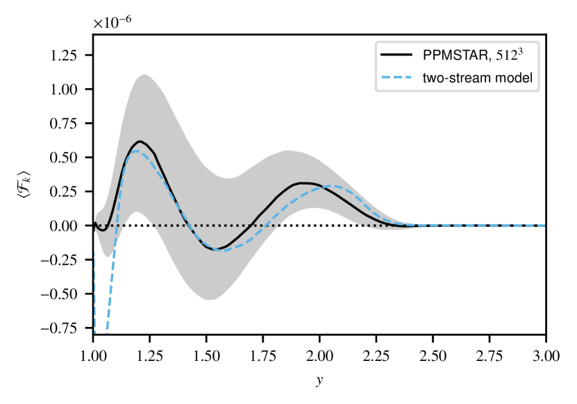
Figure 19: Profile of the kinetic-energy flux $\mathcal{F}_{\mathrm{k}}$ given by the two-stream model as compared with the actual profile of $\mathcal{F}_{\mathrm{k}}$ in the $512^{3}$ PPMSTAR run. Inputs for the two-stream model are taken from the same PPMSTAR run. The time-averaging interval and statistical-variation bands are the same as those used in Fig. 16.