Soft spin correlations in final-state parton showers

Abstract

We introduce a simple procedure that resolves the long-standing question of how to account for single-logarithmic spin-correlation effects in parton showers not just in the collinear limit, but also in the soft wide-angle limit, at leading colour. We discuss its implementation in the context of the PanScales family of parton showers, where it complements our earlier treatment of the purely collinear spin correlations. Comparisons to fixed-order matrix elements help validate our approach up to third order in the strong coupling, and an appendix demonstrates the small size of residual subleading-colour effects. To help probe wide-angle soft spin correlation effects, we introduce a new declustering-based non-global spin-sensitive observable, the first of its kind. Our showers provide a reference for its single-logarithmic resummation. The work in this paper represents the last step required for final-state massless showers to satisfy the broad PanScales next-to-leading logarithmic accuracy goals.

1 Introduction

Parton showers are some of the most extensively used tools in collider physics. For much of the past decades the main aim for parton showers, from the point of view of resummation, was to achieve leading-logarithmic (LL) accuracy, i.e. control of terms $\alpha_{s}^{n}L^{2n}$ or in some cases $\alpha_{s}^{n}L^{n+1}$, where $\alpha_{s}$ is the strong coupling and $L$ is the logarithm of a ratio of some pair of disparate momentum scales. In recent years there have been a number of advances in formulating showers with well-defined resummation accuracy Dasgupta:2018nvj ; Dasgupta:2020fwr ; Hamilton:2020rcu ; Karlberg:2021kwr ; Forshaw:2020wrq ; Holguin:2020joq ; Nagy:2020rmk ; Nagy:2020dvz , making the prospect of an NLL-accurate shower a concrete possibility. The identification of the logarithmic accuracy of tools such as a parton shower, that can be used to predict arbitrarily complex observables, is not without subtleties. One comprehensive proposal for a definition of the logarithmic accuracy was given in Refs. Dasgupta:2018nvj ; Dasgupta:2020fwr . Within that proposal, to claim NLL accuracy, a shower should correctly reproduce all sources of potential $\alpha_{s}^{n}L^{n}$ contributions, at least at leading colour. It should also reproduce tree-level matrix elements in the limits where all branchings are well separated in the Lund diagram Andersson:1988gp (these are the most common configurations and so, arguably, the configurations most likely to be targeted by machine-learning based jet-tagging methods Larkoski:2017jix ).

One fundamental set of quantum mechanical effects that has long been known to play a role in showering is that of spin correlations Webber:1986mc ; Collins:1987cp ; Knowles:1987cu . Insofar as parton showers aimed only for LL accuracy, the inclusion of spin correlations could be considered optional and of the major parton shower codes, only the Herwig showers include them fully to all orders in the collinear limit Corcella:2000bw ; Bahr:2008pv ; Bellm:2015jjp ; Richardson:2018pvo ; Webster:2019cwq . However, starting from NLL accuracy, the inclusion of spin correlations is no longer optional.

Many aspects of spin correlations can be accounted for with the Collins algorithm Collins:1987cp , which provides an efficient and straightforward approach for the spin correlations in collinear splittings. However, parton showers can involve interleaved sequences of soft, large-angle splittings and collinear splittings, and these bring in spin correlations that are beyond the scope of the Collins algorithm. As an example, Fig. 1 (left) shows configurations that contribute to single-logarithmic terms, at second order (top) and third order (bottom). In the former case, we consider the emission of a soft gluon (relative to the Born quark-pair), $E_{g_{1}}\ll E_{q},E_{\bar{q}}$, at large angle $\theta_{g_{1}}\sim 1$, where that gluon splits collinearly to either $g\to gg$ or $g\to q^{\prime}\bar{q}^{\prime}$ (in the figure, $\theta_{q^{\prime}\bar{q}^{\prime}}\ll 1$). At one order higher, we consider two gluons that are ordered in energy, $E_{g_{2}}\ll E_{g_{1}}\ll E_{q},E_{\bar{q}}$, but at commensurate, large angles, $\theta_{g_{1}}\approx\theta_{g_{2}}\sim 1$ with respect to the Born quark-pair, followed by the collinear splitting $g_{2}\to gg$, or $g_{2}\to q^{\prime}\bar{q}^{\prime}$. As in the case just of collinear splittings, the spin carried by the intermediate gluon will induce a correlation of the azimuthal angles between the successive splitting planes. This is illustrated in Fig. 1 (right).

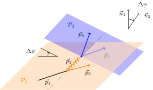
Figure 1: Left: Configurations at $\mathcal{O}(\alpha_{s}^{2})$ (top) and $\mathcal{O}(\alpha_{s}^{3})$ (bottom), where a soft, wide-angle gluon ($E_{g_{2}}\ll E_{g_{1}}\ll E_{q,\bar{q}}$ and $\theta_{g_{1}q}\sim\theta_{g_{2}q}\sim\mathcal{O}\left(1\right)$) splits collinearly ($\theta_{q^{\prime}\bar{q}^{\prime}}\ll 1$). This generates spin correlations that are sensitive to soft corrections of the type discussed in Section 2. Right: Illustration of the definition of the spin-sensitive azimuthal difference $\Delta\psi$ between subsequent branching planes.

In this article, we introduce a simple extension of the Collins algorithm, relevant for dipole showers, that enables it to simultaneously address the collinear and the soft large-angle regimes, providing an efficient solution to the last remaining barrier to obtaining an NLL-accurate massless final-state shower at leading-$N_{\text{{c}}}$ (Section 2). Section 3 presents our tests of the algorithm against fixed-order matrix elements. In Section 4 we introduce a new observable that is sensitive to the pattern of large-angle soft emissions as well as the azimuthal structure of the subsequent collinear splittings of those large-angle soft emissions. We conclude in Section 5. A number of appendices are included which provide more details on certain aspects of our work. In Appendix A we give explicit expressions for the 4- and 5-parton soft-limit matrix elements used in our validation. Appendix B discusses subleading-$N_{\text{{c}}}$ effects and Appendix C investigates the systematic effects associated with the choice of reference vector in the evaluation of spinor products.

2 Extending the Collins algorithm to the wide-angle soft limit

$\lambda_{\tilde{\imath}}$	$\lambda_{i}$	$\lambda_{k}$	$q\to qg$	$g\to q\bar{q}$	$g\to gg$
$\lambda$	$\lambda$	$\lambda$	$\frac{1}{\sqrt{1-z}}$	$0$	$\frac{1}{\sqrt{z(1-z)}}$
$\lambda$	$\lambda$	$-\lambda$	$\frac{z}{\sqrt{1-z}}$	$-z$	$\frac{z^{3/2}}{\sqrt{1-z}}$
$\lambda$	$-\lambda$	$\lambda$	$0$	$1-z$	$\frac{(1-z)^{3/2}}{\sqrt{z}}$
$\lambda$	$-\lambda$	$-\lambda$	$0$	$0$	$0$

Table 1: The helicity-dependent Altarelli-Parisi splitting amplitudes $\mathcal{F}_{{\tilde{\imath}}\to ik}^{\lambda_{\tilde{\imath}}\lambda_{i}\lambda_{k}}(z)$, where $z=E_{i}/E_{\tilde{\imath}}$.

The standard procedure for including spin correlations in a parton shower is the Collins–Knowles algorithm Collins:1987cp ; Knowles:1987cu . It relies crucially on the construction of a binary tree of $1\to 2$ collinear splittings, with strongly ordered angles as one moves down the tree, i.e. towards the shower’s final set of particles. The algorithm effectively maintains spin-density information across all nodes of the tree, and for each new $1\to 2$ splitting updates that spin-density information at all of the ancestor nodes of the splitting node. The difficulty that we face in including spin correlations for soft large-angle emissions is that the corresponding splittings necessarily involve a $2\to 3$ structure. As such they do not obviously mesh with the Collins–Knowles algorithm. We address this problem within the adaptation of the Collins–Knowles algorithm that we introduced in the PanScales framework in Ref. Karlberg:2021kwr . It was intended for use in final-state dipole and antenna showers, and we demonstrated that it correctly reproduces the spin-induced azimuthal dependence of collinear radiation in single-logarithmic terms, but did not explore the question of the soft arbitrary-angle branching.

One of the key elements of the PanScales version of the Collins–Knowles algorithm is that when an $n$-parton system undergoes a collinear ${\tilde{\imath}}\to ik$ splitting to give an $(n+1)$-parton system, the colour-stripped amplitudes ($M$) for the $(n+1)$- and $n$-parton systems can be related by collinear factorisation,

$$M^{\lambda_{i}\lambda_{k}}(\ldots,p_{i},p_{k},\ldots)=\mathcal{M}_{{\tilde{\imath}}\to ik}^{\lambda_{\tilde{\imath}}\lambda_{i}\lambda_{k}}\times M^{\lambda_{\tilde{\imath}}}(\ldots,p_{\tilde{\imath}},\ldots)\,,$$ (1)

where all helicity indices ($\lambda_{1}\ldots\lambda_{n}$) and momenta ($p_{1}\ldots p_{n}$) that are not explicitly shown remain the same on both sides. The effective splitting amplitude $\mathcal{M}_{{\tilde{\imath}}\to ik}^{\lambda_{\tilde{\imath}}\lambda_{i}\lambda_{k}}$ is given by

$$\mathcal{M}_{{\tilde{\imath}}\to ik}^{\lambda_{\tilde{\imath}}\lambda_{i}\lambda_{k}}=\frac{1}{\sqrt{2}}\frac{g_{s}}{p_{i}{\cdot}p_{k}}\mathcal{F}_{{\tilde{\imath}}\to ik}^{\lambda_{\tilde{\imath}}\lambda_{i}\lambda_{k}}(z)S_{\tau}(p_{i},p_{k})\;.$$ (2)

Here, $z$ is the momentum fraction of $i$ relative to ${\tilde{\imath}}$, while $\lambda_{a}=\pm 1$ corresponds to the helicity of parton $a$. The spinor product $S_{\tau}(p_{i},p_{k})$ (which follows the conventions of Ref. Kleiss:1985yh ) involves a complex phase that depends on the azimuth of the $ik$ angle and the spin index $\tau=\pm 1$, which is given by

$$\tau=\tilde{\lambda}_{i}+\tilde{\lambda}_{k}-\tilde{\lambda}_{\tilde{\imath}}\mbox{ where }\tilde{\lambda}=\begin{cases}\lambda/2\mbox{ for a quark},\\ \lambda\mbox{ for a gluon}.\end{cases}$$ (3)

The interplay between the phases at different nodes of the branching tree (summing over amplitude and complex-conjugate amplitude spin indices at successive splittings) ultimately leads to azimuthal correlations between splittings across the tree. The functions $\mathcal{F}_{{\tilde{\imath}}\to ik}^{\lambda_{\tilde{\imath}}\lambda_{i}\lambda_{k}}(z)$ are (real-valued) colour-stripped helicity-dependent Altarelli-Parisi splitting amplitudes, which depend on the momentum fraction $z$ carried by parton $i$, and are given in Table 1. We refer the reader to Appendix A of Ref. Karlberg:2021kwr for the derivation of Eq. 2 and further details on the conventions used in the spinor products.

Next, let us look at the analogous amplitudes in the limit where we allow the emitted gluon to be at arbitrary angles but require it to be soft relative to its parents. This involves a $2\to 3$ structure, ${\tilde{\imath}}{\tilde{\jmath}}\to ijk$, and the relation between the $n$- and $(n+1)$-parton colour-stripped amplitudes is given by Bassetto:1983mvz

$$M^{{\lambda_{k}}}(\dots,p_{i},p_{k},p_{j},\dots)=g_{s}\left(\frac{p_{i}{\cdot}\epsilon_{\lambda_{k}}^{*}(p_{k})}{p_{i}{\cdot}p_{k}}-\frac{p_{j}{\cdot}\epsilon_{\lambda_{k}}^{*}(p_{k})}{p_{j}{\cdot}p_{k}}\right)M(\dots,p_{\tilde{\imath}},p_{\tilde{\jmath}},\dots)\,.$$ (4)

As in Eq. 1, helicity indices that are not shown are the same on both sides, and in particular with regards to the ${\tilde{\imath}},i,{\tilde{\jmath}},j$ partons, there is an implicit constraint $\delta_{\lambda_{\tilde{\imath}}\lambda_{i}}\delta_{\lambda_{\tilde{\jmath}}\lambda_{j}}$. After expressing the polarisation vectors in terms of spinor products, the soft matrix element in Eq. 4 can be written as Berends:1987me

$$M^{{\lambda_{k}}}(\dots,p_{i},p_{k},p_{j},\dots)=\sqrt{2}g_{s}\frac{S_{-\lambda_{k}}(p_{i},p_{j})}{S_{-\lambda_{k}}(p_{i},p_{k})S_{-\lambda_{k}}(p_{j},p_{k})}M(\dots,p_{\tilde{\imath}},p_{\tilde{\jmath}},\dots)\,,$$ (5)

again with the implicit $\delta_{\lambda_{\tilde{\imath}}\lambda_{i}}\delta_{\lambda_{\tilde{\jmath}}\lambda_{j}}$ constraint. Using the relations

$$S_{\lambda}(p,q)=-S_{\lambda}(q,p)=-S_{-\lambda}(p,q)^{*},$$ (6a)

$$|S_{\lambda}(p,q)|^{2}=S_{\lambda}(p,q)S_{-\lambda}(q,p)=2\,p{\cdot}q,$$ (6b)

and additionally $S_{\lambda}(p_{j},p_{k})=\sqrt{(1-z)/z}S_{\lambda}(p_{j},p_{i})$ when $i$ and $k$ are collinear, it is straightforward to show that Eq. 5 reduces to the soft-collinear limit of Eqs. 1 and 2, noting that only contributions with $\lambda_{\tilde{\imath}}=\lambda_{i}$ survive in the soft ($z\to 1$) limit of Eq. 2.

For the application of the Collins–Knowles algorithm, the critical element is the factorisation structure of the helicity indices in Eq. 1. The observation that we make here is that it is possible to obtain the correct soft arbitrary-angle limit for the amplitude without modifying the factorisation of the helicity indices in Eq. 1. All that is needed to achieve this is to modify the spinor factors on the right-hand side of Eq. 2 so that the ${\tilde{\imath}}\to ik$ branching acquires a dependence on the kinematics of ${\tilde{\imath}}$’s dipole colour-partner $j$, without having to introduce any dependence on the helicity of $j$. We achieve this by replacing Eq. 2, in the case where $\lambda_{\tilde{\imath}}=\lambda_{i}$ with

$$\mathcal{M}^{\lambda\,\lambda\,\lambda_{k}}_{\tilde{\imath}\rightarrow ik}=\sqrt{2}g_{s}\mathcal{F}_{{\tilde{\imath}}\to ik}^{\lambda\,\lambda\,\lambda_{k}}(z)\sqrt{\frac{1-z}{z}}\frac{S_{-\lambda_{k}}(p_{i},p_{j})}{S_{-\lambda_{k}}(p_{i},p_{k})S_{-\lambda_{k}}(p_{j},p_{k})}\,.$$ (7)

One can also think of this as a correction factor to Eq. 2, computed as the ratio of Eq. 5 and its collinear limit. For the amplitude where $\lambda_{\tilde{\imath}}\neq\lambda_{i}$ and for $g\to q\bar{q}$ splittings, neither of which have a soft enhancement, we retain Eq. 2 as it is. It is straightforward to verify that Eq. 7 reduces to Eq. 2 in the limit where $i$ and $k$ are collinear, and to Eq. 5 when $k$ is soft, i.e. $1-z\ll 1$. When $k$ is soft and emitted from an ${\tilde{\imath}}{\tilde{\jmath}}$ dipole it is somewhat arbitrary whether to account for the emission of $k$ as an ${\tilde{\imath}}\to ik$ branching in the spin-correlation tree or as a ${\tilde{\jmath}}\to jk$ branching. That choice only makes a difference to the spin-correlation structure for contributions with $\lambda_{\tilde{\imath}}\neq\lambda_{i}$ or $\lambda_{\tilde{\jmath}}\neq\lambda_{j}$, which are both suppressed in the limit $z\to 1$, or simply zero.

The numerical evaluation of the spinor products that appear in Eq. 7 proceeds in the same fashion as was described in Appendix A of Ref. Karlberg:2021kwr . There, it was highlighted that the evaluation necessarily involves the choice of a reference spinor direction, which causes the purely collinear amplitudes to fail to reproduce the soft limit in an azimuthally-dependent way. Eq. 7 ensures that in the soft limit, the dependence on that reference direction is eliminated. We comment on this issue further in Appendix C.

A final observation is that the identification of the colour partner $j$ is only unambiguous in the large-$N_{\text{{c}}}$ limit. Accordingly, the algorithm as presented here only provides the correct soft (non-collinear) spin-correlation structures within that large-$N_{\text{{c}}}$ limit. Recall that at large angles, the PanScales showers are anyway only correct for the single (NLL) logarithms in the leading-$N_{\text{{c}}}$ limit, even if residual subleading-$N_{\text{{c}}}$ corrections have been found to be numerically small after application of the NODS colour algorithm of Ref. Hamilton:2020rcu . In Appendix B, we will further comment on the size of residual subleading-$N_{\text{{c}}}$ contributions for spin correlations.

3 Fixed-order tests

In order to demonstrate the effect of soft spin correlations, as well as the correctness of our implementation, we will show below results from the PanScales family of parton showers, at fixed order (this section) and at all orders (Section 4). As a reminder to the reader, the PanLocal shower uses a local recoil scheme, where the emission of $p_{k}$ from a dipole $\{\tilde{p}_{i},\tilde{p}_{j}\}$ is associated with the following momentum mapping,

$$p_{k} =a_{k}\tilde{p}_{i}+b_{k}\tilde{p}_{j}+k_{\perp}\,,$$ (8a)

$$p_{i} =a_{i}\tilde{p}_{i}+b_{i}\tilde{p}_{j}-fk_{\perp}\,,$$ (8b)

$$p_{j} =a_{j}\tilde{p}_{j}+b_{j}\tilde{p}_{j}-(1-f)k_{\perp}\,,$$ (8c)

with $k_{\perp}=k_{\perp,1}\cos(\varphi)+k_{\perp,2}\sin(\varphi)$ and $-k_{\perp}^{2}=k_{t}^{2}$. The Sudakov components of the emission $p_{k}$ in Eq. 8a can be expressed in terms of the evolution variable $v$ and an effective rapidity $\bar{\eta}$,

$$v=\frac{k_{t}}{\rho}e^{-\beta|\bar{\eta}|},\qquad\rho=\left(\frac{s_{{\tilde{\imath}}}s_{{\tilde{\jmath}}}}{Q^{2}s_{{\tilde{\imath}}{\tilde{\jmath}}}}\right)^{\frac{\beta}{2}}\,,\qquad a_{k}=\sqrt{\frac{s_{{\tilde{\jmath}}}}{s_{{\tilde{\imath}}{\tilde{\jmath}}}s_{{\tilde{\imath}}}}}\,k_{t}{e}^{+\bar{\eta}}\,,\qquad b_{k}=\sqrt{\frac{s_{{\tilde{\imath}}}}{s_{{\tilde{\imath}}{\tilde{\jmath}}}s_{{\tilde{\jmath}}}}}\,k_{t}{e}^{-\bar{\eta}}\,,$$ (9)

where $s_{{\tilde{\imath}}{\tilde{\jmath}}}=2{\widetilde{p}}_{i}\cdot{\widetilde{p}}_{j}$, $s_{{\tilde{\imath}}}=2{\widetilde{p}}_{i}\cdot Q$, the total momentum of the event is $Q$, and the fixed parameter $\beta$ defines the angular scaling of $v$. The other components are then fixed by requiring momentum conservation and on-shellness. The PanLocal shower comes in a dipole variant, where $f=1$, and in an antenna variant, where

$$f=f(\bar{\eta})=\frac{e^{2\bar{\eta}}}{1+e^{2\bar{\eta}}}\,.$$ (10)

The PanGlobal shower instead uses the map

$$\bar{p}_{k} =a_{k}\tilde{p}_{i}+b_{k}\tilde{p}_{j}+k_{\perp}\,,$$ (11a)

$$\bar{p}_{i} =(1-a_{k})\tilde{p}_{i}\,,$$ (11b)

$$\bar{p}_{j} =(1-b_{k})\tilde{p}_{j}\,,$$ (11c)

and applies a rescaling and Lorentz boost of all particles, including $\bar{p}_{i,j,k}$, to restore four-momentum conservation.

As part of a validation of the implementation presented above, we compare the effective differential cross section generated by the parton shower, $\text{d}\sigma_{\text{PS}}$, to the soft, leading-colour cross section, $\text{d}\sigma_{\text{Exact}}^{\text{(LC)}}$, evaluated by considering the exact matrix element in those limits at fixed order in the strong coupling $\mathcal{O}(\alpha_{s}^{2})$ and $\mathcal{O}(\alpha_{s}^{3})$. The matrix elements were computed analytically, with help from FeynCalc MERTIG1991345 ; Shtabovenko:2016sxi ; Shtabovenko:2020gxv and MultivariateApart Heller:2021qkz , using Mathematica Mathematica , in the limit where the emitted particles are much softer than the original $q\bar{q}$ pair. They were checked against matrix elements obtained using amplitudes from Refs. Nagy:1998bb ; Badger:2005jv and were found to agree at permille level in the quasi-soft limit. In principle, one could also extract the relevant limits from Refs. Catani:1999ss . The squared matrix elements are given for completeness in Appendix A. In the following, all results are shown in the large-$N_{\text{{c}}}$ limit, which is achieved in the parton shower by setting $C_{F}=\frac{1}{2}C_{A}=\frac{3}{2}$. We comment on the magnitude of subleading-colour effects in Appendix B, where the full-colour cross sections are compared with results obtained by the PanScales methods set out in Ref. Hamilton:2020rcu for including a subset of subleading-colour corrections in dipole showers.

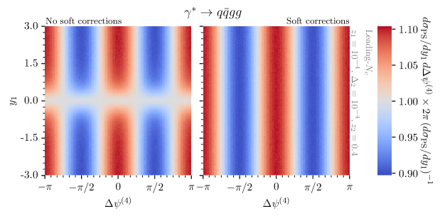
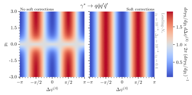
Figure 2: The double-differential cross section $d\sigma_{\text{PS}}/dy_{1}d\Delta\psi^{(4)}$ for $e^{+}e^{-}\to q\bar{q}gg$ (top) and $e^{+}e^{-}\to q\bar{q}q^{\prime}\bar{q}^{\prime}$ (bottom), without soft spin corrections (left) — i.e. purely collinear spin correlations — and with soft corrections enabled (right), normalised to the single-differential cross section $d\sigma_{\text{PS}}/dy_{1}$. Comparisons are carried out in the leading-$N_{\text{{c}}}$ approximation with $C_{F}=\frac{C_{A}}{2}=\frac{3}{2}$.

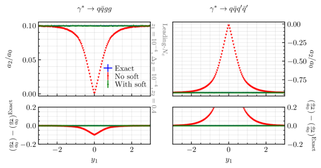
Figure 3: The extracted ratio $a_{2}/a_{0}$, as defined in Eq. 12, from the double-differential cross section of Fig. 2, as well as the exact result, as a function of $y_{1}$. Comparisons are carried out in the leading-$N_{\text{{c}}}$ approximation with $C_{F}=\frac{C_{A}}{2}=\frac{3}{2}$.

First, we examine configurations at second order, like that shown in the upper-left part of Fig. 1, where a soft, wide-angle gluon $g_{1}$ is emitted from the original $q\bar{q}$ dipole, and then splits collinearly, either as $g_{1}\to gg$ or $g_{1}\to q^{\prime}\bar{q}^{\prime}$. We fix the energy fraction carried away by the gluon $g_{1}$ in the first splitting, $z_{1}=E_{1}/Q=10^{-4}$, as well as the collinear momentum fraction and splitting angle of the second collinear branching, $z_{2}=0.4$ and $\Delta_{2}=10^{-4}$ respectively. We then sample over the rapidity $y_{1}$ of the gluon $g_{1}$, and over the azimuthal angles of both splittings. Fig. 2 shows the differential cross section, as generated by the shower, as a function of the rapidity $y_{1}$ of the emitted gluon (vertical axis) and $\Delta\psi^{(4)}$ (horizontal axis), which corresponds to the reconstructed difference in the azimuthal angles of the primary $q\to qg_{1}$ and secondary $g_{1}\to gg$, or $g_{1}\to q^{\prime}\bar{q}^{\prime}$ splitting planes (see also the right panel of Fig. 1). The upper panels are for the $\gamma^{*}\to q\bar{q}gg$ process, the lower panels are for $\gamma^{*}\to q\bar{q}q^{\prime}\bar{q}^{\prime}$. The left hand panels use just the collinear spin correlations of our earlier work Karlberg:2021kwr , while the right-hand panels show the results when we include the soft spin correlations of this work. The striking difference between left and right-hand panels is that, with the soft spin correlation corrections, the azimuthal modulation is independent of $y_{1}$, while with the pure collinear implementation of the spin correlations, that is not the case, with spurious structure appearing in the large-angle region where the shower switches between $g_{1}$ being emitted by the $q$ dipole end to it being emitted from the $\bar{q}$ dipole end. The independence on $y_{1}$ in the soft case is the correct behaviour. This is easy to understand intuitively: soft gluon emission and subsequent splitting should be invariant under longitudinal boosts along the parent ($q\bar{q}$) dipole direction.

To demonstrate that the result is indeed correct not just in structure but also normalisation, we take the Fourier cosine transform with respect to $\Delta\psi^{(4)}$, i.e. we extract the values of $a_{0}(y_{1})$ and $a_{2}(y_{1})$, following

$$\frac{d\sigma}{dy_{1}d\Delta\psi^{(4)}}=a_{0}(y_{1})+a_{2}(y_{1})\cdot\cos\big{(}2\Delta\psi^{(4)}\big{)}\,,$$ (12)

which encodes the correct azimuthal structure of spin-dependent observables Karlberg:2021kwr . Fig. 3 shows the ratio of $a_{2}/a_{0}$ for $\gamma^{*}\to q\bar{q}gg$ (left) and $\gamma^{*}\to q\bar{q}q^{\prime}\bar{q}^{\prime}$ (right) as a function of $y_{1}$, comparing to the exact result. There we see the excellent agreement of our soft-spin correlation procedure with that matrix element. Note the usual features that $g_{1}\to q^{\prime}\bar{q}^{\prime}$ splittings peak in a plane that is perpendicular to the $q\bar{q}g_{1}$ plane ($a_{2}<0$), and with a substantially stronger modulation than the $g_{1}\to gg$ splitting, which peaks in the same plane as the $q\bar{q}g_{1}$ ($a_{2}>0$).

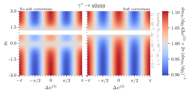
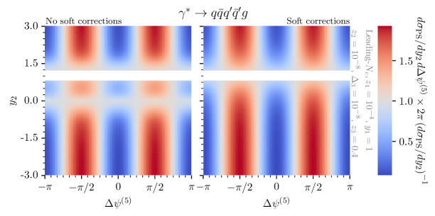
Figure 4: Same as Fig. 2 for $e^{+}e^{-}\to q\bar{q}ggg$ (top) and $e^{+}e^{-}\to q\bar{q}q^{\prime}\bar{q}^{\prime}g$ (bottom), as a function of the rapidity $y_{2}$ of a soft gluon — which then splits collinearly — and the azimuthal angle $\Delta\psi^{(5)}$ between the primary ($q\to qg_{2}$) and secondary ($g_{2}\to gg$ or $g_{2}\to q^{\prime}\bar{q}^{\prime}$) splittings. Comparisons are carried out in the leading-$N_{\text{{c}}}$ approximation with $C_{F}=\frac{C_{A}}{2}=\frac{3}{2}$.

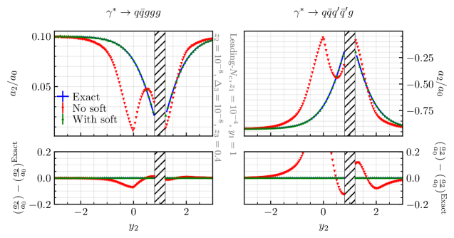
Figure 5: Same as Fig. 3, but for the configurations used in Fig. 4.

In Figs. 4 and 5, we repeat the tests for 5-parton processes, $\gamma^{*}\to q\bar{q}ggg_{1}$ and $\gamma^{*}\to q\bar{q}q^{\prime}\bar{q}^{\prime}g_{1}$, cf. Fig. 1 (lower left). We fix the rapidity of the first (non-splitting) gluon $y_{1}=1$ and its energy fraction $z_{1}=10^{-4}$ and integrate over its azimuth. The second gluon, with energy fraction $z_{2}=10^{-8}$, splits to a collinear $gg$ or $q^{\prime}\bar{q}^{\prime}$ with opening angle $\Delta_{3}=10^{-8}$. Fig. 4 shows the result of sampling over its rapidity $y_{2}$ (vertical axis) and the azimuthal angular difference between its decay plane and the $q\bar{q}g_{2}$ plane, $\Delta\psi^{(5)}$. We mask a small strip around $y_{2}\sim y_{1}$, a region that is affected by a divergence when $g_{1}$ and $g_{2}$ become collinear (this region is correctly treated by the soft spin procedure, but would be more effectively probed by a separate analysis). The corresponding results for $a_{2}/a_{0}$ are shown in Fig. 5. The exact matrix element has non-trivial structure for $y_{2}$ close to $y_{1}$, which is well reproduced by our soft-spin procedure. The purely collinear spin procedure introduces spurious structures for $y_{2}\simeq 0$ and $y_{2}\simeq y_{1}$, corresponding to the transition regions between different dipole ends.

As mentioned above, all the results shown in this section (and in the next section) are in a large-$N_{\text{{c}}}$ approximation whereby $C_{F}=C_{A}/2=3/2$. Subleading-$N_{\text{{c}}}$ corrections affect not just the intensity of soft gluon emission, but also the spin structure. The reason is that each dipole that contributes to radiating the soft gluon can transmit distinct spin information to that soft gluon. The impact of this is illustrated at fixed order in Appendix B, where we see that residual full-$N_{\text{{c}}}$ effects are numerically small, of the order of $\lesssim 1\%$ ($3\%$) for the $gg$ ($q\bar{q}$) channel with the NODS procedure.

4 A new observable sensitive to soft spin effects

Soft spin correlations are an essential requirement within the PanScales NLL conditions, and we expect that machine-learning approaches to jet analyses and substructure are likely to be learning some features of the azimuthal correlations that they induce. However, we are not aware of any existing observables that are directly sensitive to these effects. Accordingly, in this section, we propose an observable that probes both soft wide-angle and subsequent collinear splittings, and use the asymptotic limit of our parton showers to provide a reference single-logarithmic resummation for its distribution.

4.1 Definition of the observable

We start by clustering an $e^{+}e^{-}$ event, in its centre-of-mass frame, using the spherical version of the Cambridge/Aachen (C/A) algorithm Dokshitzer:1997in ; Wobisch:1998wt with $E$-scheme ($4$-momentum) recombination, as implemented in FastJet Cacciari:2011ma . We undo the steps of the clustering sequence so as to obtain exactly two jets, with momenta $p_{1}$ and $p_{2}$ and use $\vec{p}_{1}-\vec{p}_{2}$ to define the event axis direction $\hat{a}$. For each particle or jet $i$, we identify its rapidity with respect to the event direction by evaluating the $3$-momentum component parallel to $\hat{a}$, $p_{i,\hat{a}}$ and using the usual definition $y_{i}=\frac{1}{2}\ln\left((E_{i}+p_{i,\hat{a}})/(E_{i}-p_{i,\hat{a}})\right)$. We will be interested in particular in subjets that are within a slice $|y|<y_{\max}$ where $y_{\max}$ is a parameter of order $1$.

We then carry out a Lund-diagram Andersson:1988gp style analysis of the event using the $e^{+}e^{-}$ C/A declustering tree, in the spirit of Ref. Dreyer:2018nbf . The observable is defined through the following steps

1. We examine all C/A declusterings and identify any that satisfy the property that the harder subjet $j$ has $|y_{j}|>y_{\max}$ and the softer subjet $k$ has $|y_{k}|<y_{\max}$ (softer and harder are defined in terms of the magnitudes of the $3$-momenta). If there is no such declustering, the event does not contribute to the final histogram. If there is more than one declustering that satisfies that property, we choose the one with largest $k_{t}=|\vec{p}_{k}|\sin\theta_{jk}$. We denote the $k_{t}$ associated with this declustering as $k_{t,1}$ and the azimuth as $\psi_{1}$ (azimuths are defined following the procedure in Ref. Karlberg:2021kwr ).

2. Next we consider the declustering tree of $k$, and specifically all declusterings that belong to $k$’s Lund leaf (i.e. at each declustering, the softer subjet belongs to the leaf, and we then recursively continue to identify other Lund leaf subjets of $k$ by following the further declustering of the harder subjet). For each $\ell\to mn$ declustering, we evaluate $z=|\vec{p}_{n}|/(|\vec{p}_{m}|+|\vec{p}_{n}|)$ where $n$ is the softer branch. We identify all declusterings with $z$ larger than some parameter $z_{\text{cut}}$. If there are none, the event does not contribute to the final histogram. If there is more than one, we choose the one with largest $k_{t}$, which we denote as $k_{t,2}$. We denote its azimuth as $\psi_{2}$.

3. Finally, for all events with $k_{t,2}>k_{t,\text{min}}$, we bin the distribution of the signed azimuthal angle $\Delta\psi_{12}^{\mathrm{slice}}\equiv\psi_{2}-\psi_{1}$ between the two splitting planes identified above.

An illustration of how this observable works at the first non-zero order, $\alpha_{s}^{2}$, is given in Fig. 6, which shows a primary emission $g_{1}$ within the $y_{\max}$ rapidity constraint and its subsequent collinear splitting to a $q^{\prime}\bar{q}^{\prime}$ pair with $z>z_{\text{cut}}$. In this simple case, $\Delta\psi_{12}^{\mathrm{slice}}$ is the difference in azimuthal angle between the $g_{1}q$ plane and the $q^{\prime}\bar{q}^{\prime}$ plane. Code to evaluate the observable will be distributed as part of the LundPlane FastJet contrib package.

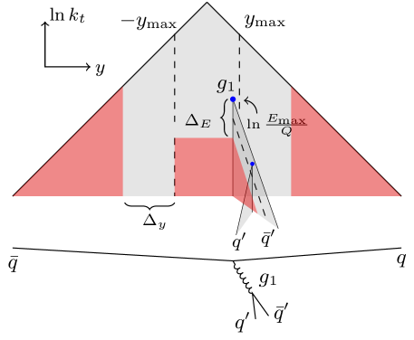
Figure 6: For the definition of the slice observable $\Delta\psi_{12}^{\mathrm{slice}}$, we consider primary splittings $q\to qg_{1}$ whose softer branch is found in a central rapidity slice $[-y_{\text{max}},y_{\text{max}}]$. Following that softer branch, we select secondary splittings that satisfy $z\geq z_{\text{cut}}$. The cuts are indicated by dashed lines on the Lund plane. The red shaded patches illustrate the regions where shower emissions may be vetoed in the limit of $\alpha_{s}\rightarrow 0$ at a fixed $\lambda=\alpha_{s}L$.

At order $\mathcal{O}(\alpha_{s}^{2})$, the leading-$N_{\text{{c}}}$ contribution to the slice observable is given by

$$\frac{d\sigma^{\text{FO}}}{d\Delta\psi_{12}^{\mathrm{slice}}}=|M_{q\bar{q}}|^{2}\,2y_{\text{max}}\left(\frac{\alpha_{s}}{\pi}\right)^{2}C_{F}\,\text{ln}^{2}\left(\frac{k_{t,\text{min}}}{Q}\right)\\ \times\int_{z_{\text{cut}}}^{1-z_{\text{cut}}}\text{d}z_{2}\mathcal{P}_{kg}(z_{2})\big{[}1+B_{kg}(z_{2})\cos\left(2\Delta\psi_{12}^{\mathrm{slice}}\right)\big{]}\,,$$ (13)

with $\mathcal{P}_{kg}(z)$ the usual leading-order unregularised DGLAP splitting functions, with their symmetry factors, where $k\in\{g,q\}$ refers to the secondary splitting, $g_{1}\to gg$ or $g_{1}\to q\bar{q}$, and the $B_{kg}(z)$ as given in Ref. Karlberg:2021kwr ,

$$\mathcal{P}_{gg}(z) =C_{A}\left(\frac{z}{1-z}+\frac{1-z}{z}+z(1-z)\right), B_{gg}(z) =\frac{z^{2}(1-z)^{2}}{(1-z(1-z))^{2}}\,,$$ (14)

$$\mathcal{P}_{qg}(z) =T_{R}n_{f}(z^{2}+(1-z)^{2}), B_{qg}(z) =\frac{-2z(1-z)}{1-2z(1-z)}\,.$$ (15)

The relative azimuthal modulations are maximal for $z=1/2$, and therefore adjusting $z_{\text{cut}}$ in Eq. 13 affects their ultimate observed size.

At all orders, the dominant logarithmically enhanced terms for this observable are single-logarithmic contributions $\alpha_{s}^{n}L^{n}$ with $L=\ln k_{t,\min}/Q$. The single-logarithmic resummation for the observable has the structure

$$\frac{1}{\sigma}\frac{d\sigma}{d\Delta\psi_{12}^{\mathrm{slice}}}=a_{0}(\alpha_{s}L)+a_{2}(\alpha_{s}L)\cdot\cos\left(2\Delta\psi_{12}^{\mathrm{slice}}\right)+\mathcal{O}\left(\alpha_{s}^{n}L^{n-1}\right)\,.$$ (16)

The resummation for the analogous, purely collinear $\Delta\psi_{12}$ of Ref. Karlberg:2021kwr could be obtained using a collinear spin extension of the MicroJets code Dasgupta:2014yra ; Dasgupta:2016bnd . This then served to validate the PanScales shower at single-logarithmic order. The MicroJets code cannot, however, be used for soft spin effects. Instead, for the validation of our implementation of soft-spin effects in the PanScales showers, we rely on the fixed-order tests of Section 3. Here we use the PanScales showers to determine a reference resummation for the soft-spin observable.

4.2 Strategy for resummation with the PanScales showers

As in previous PanScales work, our strategy to obtain the resummed result for the soft-spin observable is to consider the limit where we take the strong coupling constant $\alpha_{s}\to 0$, with $\alpha_{s}\ln k_{t,\min}/Q$ held fixed. In practice, we use a fixed small value of the $\alpha_{s}(Q)=10^{-7}$ with 1-loop running (with $n_{f}=5$ light flavours), for different values of $\lambda=\alpha_{s}L$.

Running the PanScales showers at such small values of $\alpha_{s}$ and large values of the logarithm is made possible by the techniques described in Appendix D of Ref. Karlberg:2021kwr . Additionally, in order to maintain computationally manageable multiplicities, Ref. Karlberg:2021kwr ran the shower in a version where soft emissions were vetoed. This could be done safely, as the observables under consideration were only sensitive to collinear emissions. On the other hand, $\Delta\psi_{12}^{\mathrm{slice}}$ is also sensitive to soft emissions in the slice and removing all soft emissions would yield the incorrect results. Instead, therefore, we allow emissions to be generated if either they are at (absolute) rapidity with respect to either dipole parent that is below some threshold $|y|<\Delta_{y}+y_{\text{max}}$ ($\Delta_{y}$ should be taken substantially larger than the rapidity $y_{\text{max}}$ of the slice with respect to the event axis), or if the parent is in the slice and the emission has an energy that is above some threshold $\ln E/Q>\Delta_{E}+\ln E_{\text{max}}/Q$, where $E_{\text{max}}$ is the energy of the highest-energy emission in the slice. This is illustrated in Fig. 6. We have verified that if we work at finite values of $\alpha_{s}$ and $\ln k_{t,\min}/Q$, results with and without these vetoes are identical to within statistics.

One further subtlety concerns the handling of flavour. As we have seen at fixed order, soft spin correlation effects depend strongly on the flavour structure of the ultimate collinear splitting that we examine and it is of interest to present resummed results separated according to the flavour structure. In Ref. Karlberg:2021kwr , to separate channels we kept track of the flavour of emitted particles in the spin correlation tree itself. Here we take a different approach: we identify the flavour of pseudo-jets appearing in the Lund declustering sequence by summing the flavours of the individual constituents. This definition of flavour is infrared unsafe, with the infrared divergence contributing at order $\alpha_{s}^{n}\ln^{n-1}k_{t,\text{cut}}/Q$ where $k_{t,\text{cut}}$ is the shower’s infrared cutoff. In most circumstances this prevents the use of flavour in conjunction with the Cambridge/Aachen algorithm. However, in our study here, we consider the limit $\alpha_{s}\to 0$ with $\alpha_{s}\ln k_{t,\min}/Q$ held fixed. Furthermore, in this limit we are free to choose $k_{t,\text{cut}}\sim k_{t,\min}$. This ensures that the formally divergent terms $\alpha_{s}^{n}\ln^{n-1}k_{t,\text{cut}}/Q$ actually vanish in our $\alpha_{s}\to 0$ limit. This is a feature that we can exploit only for studies at single-logarithmic level. Were we to examine further subleading logarithms, we would need to identify an alternative approach to flavour.

Given the net flavour of the pseudo-jets appearing in the Lund declustering sequence, we assign a secondary declustering to:

• the $gg$ channel, if both the harder and softer branches of the secondary declustering are flavourless,

• the $q\bar{q}$ channel, if each of the two prongs has the net flavour of a single quark or anti-quark, and the sum of those prongs has no net flavour,

• the rest channel, otherwise (which mainly involves $q\to qg$ splittings).

Unless specified, the results that we will show are obtained with the PanGlobal shower with $\beta=0$.

4.3 Resummed results

All-order results for the observable $\Delta\psi_{12}^{\mathrm{slice}}$ are displayed in Fig. 7 for $\lambda=\alpha_{s}\ln k_{t,\min}/Q=-0.5$, where the central rapidity slice is given by $|y_{1}|<y_{\text{max}}=1$ and the cut on the energy fraction of the secondary splitting is $z_{2}>z_{\text{cut}}=0.1$. For the individual emission vetoes described above, we choose $\Delta_{y}=9$, $\Delta_{E}=-10$. We use the leading-$N_{\text{{c}}}$ limit of $C_{F}=C_{A}/2=3/2$. Results are shown for all flavour channels combined (top left), and separately in the $g\to gg$ (top right), $g\to q\bar{q}$ (bottom left) and “rest” channels (bottom right). In the case where no spin correlations are applied (grey bullets), all curves show a uniform distribution in $\Delta\psi_{12}^{\mathrm{slice}}$. If the purely-collinear spin correlations are enabled, but without soft corrections (red triangles), we observe an azimuthal modulation of order $\sim 1.4\%$ in the distribution where all splitting channels are summed. Once the soft corrections are enabled (green triangles), the spin correlations have a distinctly larger effect, with a modulation of $\sim 2.8\%$ in the all-channels distribution ($58\%$ in the $g\to q\bar{q}$ channel). For comparison, we also show the distribution obtained at second order (blue line), rescaled so that its mean value coincides with the mean value of the all-order result. It helps to illustrate that relative to that fixed-order result, the resummation leads to a modest reduction in the degree of spin correlations (it also affects the overall normalisation, reducing it by 22% compared to the fixed order). Our interpretation of this observation is that, as in the purely collinear case Karlberg:2021kwr , the spin correlations are partly washed out by the resummation, as spin information is scattered across the event by multiple gluon emissions along the declustering sequence.

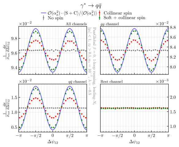
Figure 7: All-order comparison for the $\Delta\psi_{12}^{\mathrm{slice}}$ observable defined in the text for $\gamma^{*}\rightarrow q\bar{q}$. The four panels show the combination of all flavour channels for the splitting in the slice (upper left), the $g\rightarrow gg$ channel (upper right), the $g\rightarrow q\bar{q}$ channel (lower left), and a remainder channel where the splitting is classified neither as $gg$ nor $q\bar{q}$ (lower right). The plots show the predictions without spin correlations (grey dots), with the collinear spin correlations of Ref. Karlberg:2021kwr (red triangles), and with the soft gluon corrections of this work (green triangles). The blue curve is the $\mathcal{O}(\alpha_{s}^{2})$ result, rescaled so that its mean value coincides with the all-order result. The results are produced with the PanGlobal shower, with $\beta=0$, in a leading-$N_{\text{{c}}}$ approximation with $C_{F}=\frac{C_{A}}{2}=\frac{3}{2}$, and using $\lambda\equiv\alpha_{s}L=-0.5$.

In Fig. 8 we compare the PanGlobal shower with $\beta=0$ to the dipole and antenna versions of the PanLocal shower with $\beta=0.5$. Given that we do not know the analytical resummation of the $\Delta\psi_{12}^{\mathrm{slice}}$ observable, this is an important cross-check that no subleading logarithmic effects are present in our setup, and helps give us confidence that our implementation reproduces the correct all-order structure.

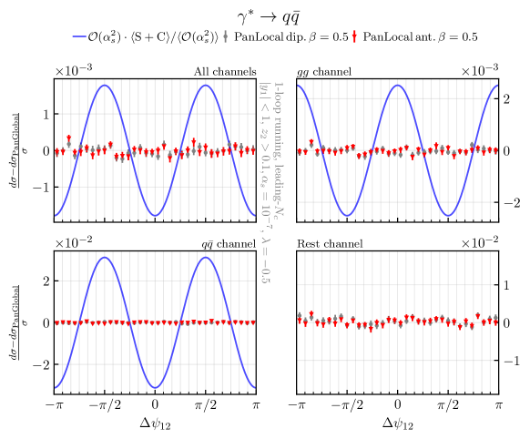
Figure 8: Same as Fig. 7, but where the all-order results with soft spin corrections are produced by two different PanScales showers, PanLocal dipole with $\beta=0.5$ (grey) and PanLocal antenna with $\beta=0.5$ (red). Instead of the normalised cross section, we show the normalised difference with respect to the PanGlobal $\beta=0$ results of Fig. 7.

To provide reference results for future studies, in Table 2 we consider three values of $\lambda=-0.5,-0.25$ and $-0.125$ and show the values of the coefficients $a_{0}$ and $a_{2}$, as defined in Eq. 16, and extracted through a Fourier cosine transform. The results are given separately for the sum over flavour channels and for the $g\to gg$ and $g\to q\bar{q}$ splitting channels. The magnitude of the rest channel can be deduced from the difference and has an $a_{2}$ value that is consistent with zero.

$\lambda$	$-0.5$	$-0.25$	$-0.125$
	All channels
$a_{0}$	$+9.63\cdot 10^{-2}$	$+2.80\cdot 10^{-2}$	$+7.34\cdot 10^{-3}$
$a_{2}$	$-2.68\cdot 10^{-3}$	$-8.30\cdot 10^{-4}$	$-2.24\cdot 10^{-4}$
$a_{2}/a_{0}$	$-2.78\cdot 10^{-2}$	$-2.96\cdot 10^{-2}$	$-3.05\cdot 10^{-2}$

	$gg$
$a_{0}$	$+8.33\cdot 10^{-2}$	$+2.45\cdot 10^{-2}$	$+6.44\cdot 10^{-3}$
$a_{2}$	$+4.01\cdot 10^{-3}$	$+1.25\cdot 10^{-3}$	$+3.36\cdot 10^{-4}$
$a_{2}/a_{0}$	$+4.81\cdot 10^{-2}$	$+5.10\cdot 10^{-2}$	$+5.22\cdot 10^{-2}$

	$q\bar{q}$
$a_{0}$	$+1.14\cdot 10^{-2}$	$+3.35\cdot 10^{-3}$	$+8.82\cdot 10^{-4}$
$a_{2}$	$-6.69\cdot 10^{-3}$	$-2.08\cdot 10^{-3}$	$-5.60\cdot 10^{-4}$
$a_{2}/a_{0}$	$-5.86\cdot 10^{-1}$	$-6.20\cdot 10^{-1}$	$-6.35\cdot 10^{-1}$

Table 2: Numerical values of the coefficients $a_{0}$, $a_{2}$, as defined in Eq. (16), and the size of the spin correlations $a_{2}/a_{0}$ for the observable $\Delta\psi_{12}^{\mathrm{slice}}$ ($y_{\text{max}}=1,\,z_{\text{cut}}=0.1$), as extracted by a Fourier cosine transform from the PanGlobal $\beta=0$ shower with soft corrections included, for values of $\lambda\equiv\alpha_{s}L\in\{-0.5,-0.25,-0.125\}$. The contributions are given separately for each flavour channel, and their statistical uncertainty is at most one in the last quoted digit for all results. We employ the leading-$N_{\text{{c}}}$ approximation with $C_{F}=\frac{C_{A}}{2}=\frac{3}{2}$.

The ratio $a_{2}/a_{0}$ is furthermore shown in Fig. 9 as a function of $\lambda$, where the fixed-order result is also included, see Eq. 13. The size of the modulation $a_{2}/a_{0}$ decreases approximately linearly with $\lambda$ in all three figures, and approaches the fixed-order result for $\lambda\rightarrow 0$ as expected. A fit of the points confirms that there are also non-linear terms present, with small numerical coefficients.

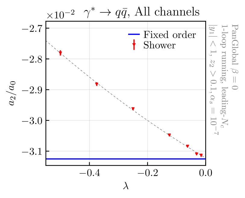
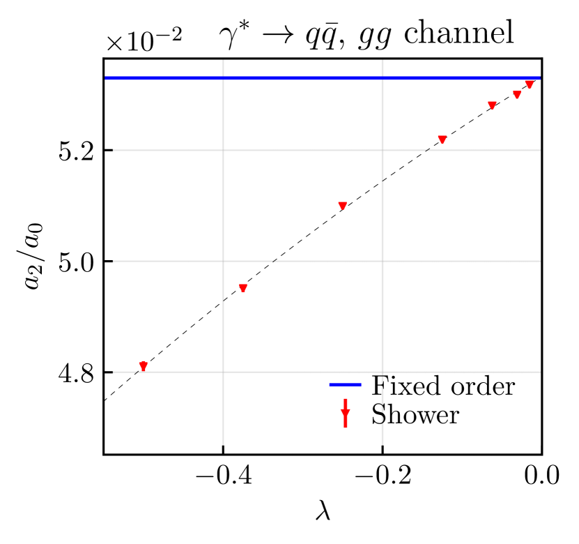
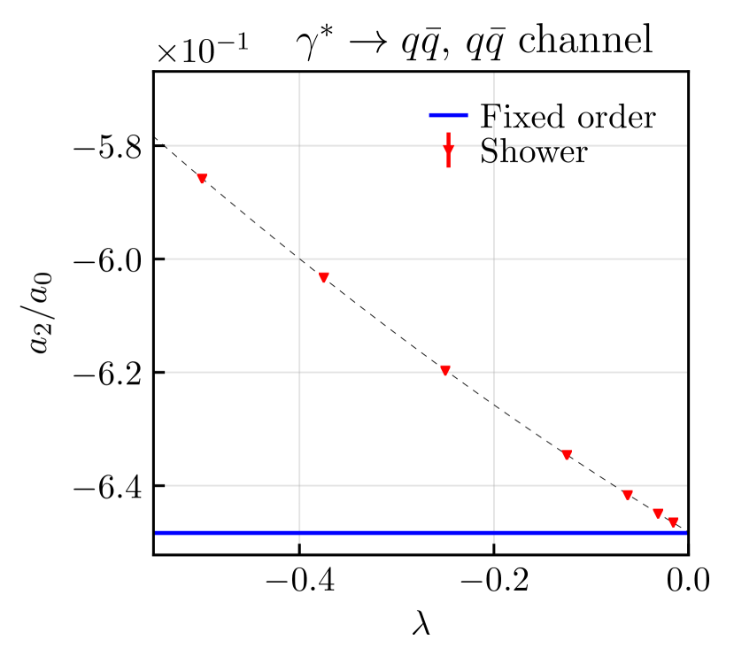
Figure 9: The ratio $a_{2}/a_{0}$ as a function of $\lambda=\alpha_{s}L$ for $\alpha_{s}=10^{-7}$. In red we show the PanGlobal shower with $\beta=0$ and in blue the (integrated) analytic fixed-order result, see Eq. 13. The three panels show all channels (upper), the channel where a $g\rightarrow gg$ splitting is found inside the slice (lower left) and the channel where a $g\rightarrow q\bar{q}$ splitting is found inside the slice (lower right). The size of the modulation $a_{2}/a_{0}$ decreases with $\lambda$ in all three plots, and approaches the fixed order result for $\lambda\rightarrow 0$. We use the leading-$N_{\text{{c}}}$ approximation with $C_{F}=\frac{C_{A}}{2}=\frac{3}{2}$.

5 Conclusions

We have demonstrated in this article that it is relatively straightforward to extend the Collins-Knowles algorithm for collinear spin correlations so as to address also the spin correlations of soft emissions, in the leading-$N_{\text{{c}}}$ limit. Within the PanScales shower framework, this was the last step needed to obtain massless final-state showers that fully satisfy the PanScales NLL conditions at leading-$N_{\text{{c}}}$. In particular it is critical for reproducing the correct azimuthal structure of matrix elements of nested sequences of soft and then collinear splittings, regardless of the angle of the soft splitting. Within the frame of an individual dipole, the structure of the spin correlations for soft emissions is remarkably simple, as it has to be given the invariance of soft emission with respect to boosts along the parent dipole direction, cf. Fig. 2 (right). A purely collinear implementation of the spin correlations, e.g. that of our earlier work Karlberg:2021kwr , can alter that simple structure with $\mathcal{O}\left(1\right)$ relative artefacts at angles commensurate with parent-dipole opening angles.

Beyond the leading-$N_{\text{{c}}}$ limit, it would no longer be sufficient to consider a single parent dipole for any given large-angle soft emission. This would complicate the treatment of soft spin correlations in the same way that it complicates the treatment of soft emission more generally. In principle one could adapt the NODS colour treatment of Ref. Hamilton:2020rcu to also address spin correlations up to some fixed order. However, we leave this to future work, especially in view of the observation in Appendices A and B that the original spin-agnostic NODS approach, combined with our leading-$N_{\text{{c}}}$ soft spin correlations, already reproduces the full-colour $3$-emission matrix elements’ azimuthal modulation to within a few percent.

As was the case until recently Chen:2020adz ; Karlberg:2021kwr also for collinear spin correlations, there are, to our knowledge, no standard observables geared to the measurement of soft spin correlations. The observable that we introduce in Section 4 addresses this gap. Our showers provide reference resummations for this observable, cf. Figs. 7 and 9 and Table 2.

Overall, spin correlations in the soft limit lead to significant azimuthal modulations, and may be important also in work towards higher-order parton showers (see, for example, the discussion in Ref. Gellersen:2021eci ). We hope that our results can pave the way to their straightforward inclusion in a range of parton showers.

Appendix A Analytic matrix elements

We write out below the matrix elements calculated analytically for emissions from the Born $\gamma^{*}\to q\bar{q}$ at second and third order, which are used in the comparisons performed in Section 3. We will use the following auxiliary functions for the different emission terms:

$$\mathcal{A}_{3}(a,b,c)= \frac{4s_{a,c}}{s_{a,b}s_{b,c}}\,,$$ (17)

$$\mathcal{A}_{4}(a,b,c,d)= \frac{8s_{a,d}^{2}}{s_{a,b}s_{c,d}\left(s_{a,b}+s_{a,c}\right)\left(s_{b,d}+s_{c,d}\right)}+\frac{8s_{a,d}}{s_{a,b}s_{b,c}}\left(\frac{1}{s_{c,d}}+\frac{1}{s_{b,d}+s_{c,d}}\right)$$

$$+ \frac{8s_{a,d}}{s_{b,c}\left(s_{a,b}+s_{a,c}\right)}\left(\frac{1}{s_{c,d}}-\frac{4}{s_{b,d}+s_{c,d}}\right)$$

$$+ \frac{2}{s_{b,c}^{2}}\left(\frac{s_{a,b}-s_{a,c}}{s_{a,b}+s_{a,c}}-\frac{s_{b,d}-s_{c,d}}{s_{b,d}+s_{c,d}}\right)^{2}\,,$$ (18)

$$\delta(q,\bar{q}\,;\,a,b,c)\,=\, \mathcal{A}_{4}(q,c,b,\bar{q})\,+\,\mathcal{A}_{3}(q,b,\bar{q})\,\mathcal{A}_{3}(q,c,a)$$

$$+\, \mathcal{A}_{3}(q,c,\bar{q})\,\mathcal{A}_{3}(q,b,a)-\,\frac{1}{2}\,\mathcal{A}_{3}(q,b,\bar{q})\,\mathcal{A}_{3}(q,c,\bar{q})\,,$$ (19)

with the Lorentz invariant $s_{i,j}=2p_{i}\cdot p_{j}$. Furthermore, we will express the matrix elements for final states containing a quark pair $q^{\prime},\,\bar{q}^{\prime}$ below, with the help of the following functions:

$$\mathcal{B}_{2}(a,b\,;\,q^{\prime},\bar{q}^{\prime})= \frac{2}{s_{q^{\prime},\bar{q}^{\prime}}}\,\bigg{(}\frac{s_{a,b}}{\left(s_{a,q^{\prime}}+s_{a,\bar{q}^{\prime}}\right)\left(s_{b,q^{\prime}}+s_{b,\bar{q}^{\prime}}\right)}$$

$$- \frac{1}{4s_{q^{\prime},\bar{q}^{\prime}}}\left(\frac{s_{a,q^{\prime}}-s_{a,\bar{q}^{\prime}}}{s_{a,q^{\prime}}+s_{a,\bar{q}^{\prime}}}-\frac{s_{b,q^{\prime}}-s_{b,\bar{q}^{\prime}}}{s_{b,q^{\prime}}+s_{b,\bar{q}^{\prime}}}\right)^{2}\,\bigg{)}\,,$$ (20)

$$\mathcal{B}_{3}(a,b,c\,;\,q^{\prime},\bar{q}^{\prime})\,=\, \frac{1}{s_{a,b}}\,\bigg{(}\,\big{(}\frac{s_{a,b}}{(s_{a,q^{\prime}}+s_{a,\bar{q}^{\prime}})(s_{b,q^{\prime}}+s_{b,\bar{q}^{\prime}})}+\frac{s_{a,c}}{(s_{a,q^{\prime}}+s_{a,\bar{q}^{\prime}})(s_{c,q^{\prime}}+s_{c,\bar{q}^{\prime}})}$$

$$- \frac{s_{b,c}}{(s_{b,q^{\prime}}+s_{b,\bar{q}^{\prime}})(s_{c,q^{\prime}}+s_{c,\bar{q}^{\prime}})}\big{)}$$

$$- \frac{1}{2s_{q^{\prime},\bar{q}^{\prime}}}\big{(}\frac{s_{a,q^{\prime}}-s_{a,\bar{q}^{\prime}}}{s_{a,q^{\prime}}+s_{a,\bar{q}^{\prime}}}-\frac{s_{b,q^{\prime}}-s_{b,\bar{q}^{\prime}}}{s_{b,q^{\prime}}+s_{b,\bar{q}^{\prime}}}\big{)}\,\big{(}\frac{s_{a,q^{\prime}}-s_{a,\bar{q}^{\prime}}}{s_{a,q^{\prime}}+s_{a,\bar{q}^{\prime}}}-\frac{s_{c,q^{\prime}}-s_{c,\bar{q}^{\prime}}}{s_{c,q^{\prime}}+s_{c,\bar{q}^{\prime}}}\big{)}\,\bigg{)}\,.$$ (21)

The 4-parton matrix element for $\gamma^{*}\to q\bar{q}g_{1}g_{2}$

We assume the following ordering in the energies of the final-state gluons:

• the energy of the two gluons $g_{1}$ and $g_{2}$ is much smaller than the energies of the Born (anti-)quark, $E_{g_{1}},E_{g_{2}}\ll E_{q},E_{\bar{q}}$ (no ordering is assumed on the relative energy of the two gluons).

The matrix element at leading colour is given by

$$\lim_{\begin{subarray}{c}N_{\text{{c}}}\rightarrow\infty\end{subarray}}\,\frac{\left|\mathscr{M}_{q\bar{q}g_{1}g_{2}}\right|^{2}}{\left|\mathscr{M}_{q\bar{q}}\right|^{2}} =\ \left(4\pi\alpha_{{\scriptscriptstyle S}}\right)^{2}\left(\frac{N_{\text{{c}}}}{2}\right)^{2}\big{(}\mathcal{A}_{4}(q,g_{1},g_{2},\bar{q})+\mathcal{A}_{4}(q,g_{2},g_{1},\bar{q})\big{)}\,.$$ (22)

The 5-parton matrix element for $\gamma^{*}\to q\bar{q}g_{1}g_{2}g_{3}$

We assume the following ordering in the energies of the final-state gluons:

• the energy of the first gluon $g_{1}$ is much smaller than the energies of the Born quarks, $E_{g_{1}}\ll E_{q},E_{\bar{q}}$

• the energies of the second and third gluons, $g_{2}$ and $g_{3}$, are much smaller than the energy of the first gluon, $E_{g_{2}},E_{g_{3}}\ll E_{g_{1}}$ (no ordering is assumed on the relative energy of $g_{2}$ and $g_{3}$).

We first give the matrix element at leading colour,

$$\lim_{\begin{subarray}{c}N_{\text{{c}}}\rightarrow\infty\end{subarray}}\,\frac{\left|\mathscr{M}_{q\bar{q}g_{1}g_{2}g_{3}}\right|^{2}}{\left|\mathscr{M}_{q\bar{q}}\right|^{2}}= \ \left(4\pi\alpha_{{\scriptscriptstyle S}}\right)^{3}\left(\frac{N_{\text{{c}}}}{2}\right)^{3}\mathcal{A}_{3}(q,g_{1},\bar{q})$$

$$\times \ \left(\mathcal{A}_{3}(q,g_{3},g_{1})\mathcal{A}_{3}(g_{1},g_{2},\bar{q})+\mathcal{A}_{4}(q,g_{2},g_{3},g_{1})+\mathcal{A}_{4}(g_{1},g_{2},g_{3},\bar{q})\right)$$

$$+ \ \{g_{2}\leftrightarrow g_{3}\}\,.$$ (23)

At full colour, $N_{C}=3$, the matrix element is corrected to:

$$\frac{\left|\mathscr{M}_{q\bar{q}g_{1}g_{2}g_{3}}\right|^{2}}{\left|\mathscr{M}_{q\bar{q}}\right|^{2}}\,=\, \left(\frac{2C_{F}}{C_{A}}\right)\,\lim_{\begin{subarray}{c}N_{{\scriptscriptstyle C}}\rightarrow\infty\end{subarray}}\,\frac{\left|\mathscr{M}_{q\bar{q}g_{1}g_{2}g_{3}}\right|^{2}}{\left|\mathscr{M}_{q\bar{q}}\right|^{2}}\,$$

$$- \left(\frac{2C_{F}}{C_{A}}\right)\,\left(4\pi\alpha_{{\scriptscriptstyle S}}\right)^{3}\,\frac{N_{\text{{c}}}}{8}\,\mathcal{A}_{3}(q,g_{1},\bar{q})\,\left(\delta(q,\bar{q}\,;\,g_{1},g_{2},g_{3})\,+\delta(\bar{q},q\,;\,g_{1},g_{2},g_{3})\,\right)\,$$

$$+ \left(\frac{2C_{F}}{C_{A}}\right)\,\left(4\pi\alpha_{{\scriptscriptstyle S}}\right)^{3}\,\frac{1}{8N_{\text{{c}}}}\,\mathcal{A}_{3}(q,g_{1},\bar{q})\,\mathcal{A}_{3}(q,g_{2},\bar{q})\,\mathcal{A}_{3}(q,g_{3},\bar{q})\,.$$ (24)

The matrix element given in Eq. (24) is the one used in the comparisons to the NODS scheme presented in Appendix B.

The 4-parton matrix element for $\gamma^{*}\to q\bar{q}q^{\prime}\bar{q}^{\prime}$

We assume the following ordering in the energies of the final-state quarks:

• the energy of the two quarks $q^{\prime}$ and $\bar{q}^{\prime}$ is much smaller than the energies of the Born quarks, $E_{q^{\prime}},E_{\bar{q}^{\prime}}\ll E_{q},E_{\bar{q}}$.

The matrix element, exact in $N_{C}$, is given by

$$\frac{\left|\mathscr{M}_{q\bar{q}q^{\prime}\bar{q}^{\prime}}\right|^{2}}{\left|\mathscr{M}_{q\bar{q}}\right|^{2}}\,= \left(4\pi\alpha_{s}\right)^{2}\,4n_{f}T_{R}C_{F}\,\mathcal{B}_{2}(q,\bar{q}\,;\,q^{\prime},\bar{q}^{\prime})\,.$$ (25)

The 5-parton matrix element for $\gamma^{*}\to q\bar{q}q^{\prime}\bar{q}^{\prime}g$

We assume the following ordering in the energies of the final-state particles:

• the energy of the gluon $g$ is much smaller than the energies of the Born quarks, $E_{g}\ll E_{q},E_{\bar{q}}$.

• the energy of the two quarks $q^{\prime}$ and $\bar{q}^{\prime}$ is much smaller than the energy of the gluon, $E_{q^{\prime}},E_{\bar{q}^{\prime}}\ll E_{g}$

The matrix element, exact in $N_{C}$, is given by

$$\frac{\left|\mathscr{M}_{q\bar{q}q^{\prime}\bar{q}^{\prime}g}\right|^{2}}{\left|\mathscr{M}_{q\bar{q}}\right|^{2}}= \left(4\pi\alpha_{s}\right)^{3}\,4n_{f}T_{R}\,\left(\frac{N_{C}}{2}\right)^{2}\,\mathcal{A}_{3}(q,g,\bar{q})$$

$$\times \bigg{(}\mathcal{B}_{2}(q,g\,;\,q^{\prime},\bar{q}^{\prime})-\frac{1}{N_{C}^{2}}\left(4\mathcal{B}_{3}(q,g,\bar{q}\,;\,q^{\prime},\bar{q}^{\prime})+\mathcal{B}_{3}(g,q,\bar{q}\,;\,q^{\prime},\bar{q}^{\prime})-\mathcal{B}_{2}(q,\bar{q}\,;\,q^{\prime},\bar{q}^{\prime})\right)$$

$$+ \frac{1}{2N_{C}^{4}}\left(4\mathcal{B}_{3}(q,g,\bar{q}\,;\,q^{\prime},\bar{q}^{\prime})-\mathcal{B}_{2}(q,\bar{q}\,;\,q^{\prime},\bar{q}^{\prime})\right)\bigg{)}$$

$$+ \left\{q\leftrightarrow\bar{q}\right\}\,.$$ (26)

The full-colour matrix element in Eq. (26) is used in the comparisons to the NODS results in Appendix B. In the limit $N_{C}\to\infty$, only the first term in the parenthesis remains.

Appendix B Fixed-order tests at full colour

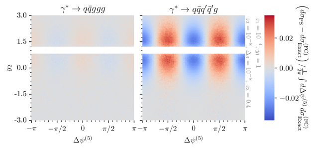
Figure 10: The ratio $\left(\text{d}\sigma_{\text{PS}}-\text{d}\sigma_{\text{Exact}}^{\text{(FC)}}\right)/\frac{1}{2\pi}\int{\Delta\psi^{(5)}\text{d}\sigma_{\text{Exact}}^{\text{(FC)}}}$ of the difference between the parton shower and the correct squared full colour tree-level matrix element, for $e^{+}e^{-}\to q\bar{q}ggg$ (left) and $e^{+}e^{-}\to q\bar{q}q^{\prime}\bar{q}^{\prime}g$ (right), for the azimuthal correlation between the primary and secondary splitting planes $\Delta\psi^{(5)}$. The parton shower result is shown using the NODS method of Ref. Hamilton:2020rcu .

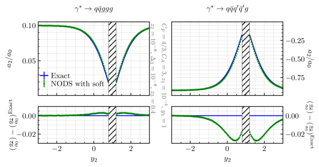
Figure 11: The ratio $a_{2}/a_{0}$ extracted from the double-differential cross section in Fig. 10, as a function of $y_{2}$, comparing the NODS-enhanced soft-spin algorithm with the full-colour (squared) matrix-element results from Appendix A.

In the main body of the paper, we have considered only the leading-colour approximation by setting $C_{F}=C_{A}/2=3/2$, as we do not expect our implementation of spin correlations to reproduce the full-colour structure at NLL.

Here we consider the performance of our method beyond the leading-$N_{\text{{c}}}$ limit, in the context of the NODS (nested ordered double-soft) scheme for including subleading-colour effects in parton showers at leading-logarithmic level, as introduced in Ref. Hamilton:2020rcu . The NODS scheme consists of a local (squared) matrix-element correction, which ensures that the shower reproduces the correct full-colour radiation pattern for every pair of soft energy-ordered commensurate-angle gluons, as long as other emissions are well-separated from that pair, in rapidity. In the tests that we show here, we use the large-$N_{\text{{c}}}$ soft-spin approach of Section 2, multiplied by the spin-averaged subleading-$N_{\text{{c}}}$ NODS correction factors.

In Figs. 10 and 11, we compare the full-colour matrix element against the dipole version of the PanLocal shower (with $\beta=0.5$) using the NODS procedure, for the same 5-parton configurations as those presented in Section 3. Note that the results presented here are independent of the exact PanScales shower choice. For a soft gluon emission at rapidities close to the (fixed) first gluon rapidity, $y_{2}\sim y_{1}$, the parton-shower result does not reproduce the correct azimuthal dependence at full colour, though it does generate the correct azimuth-integrated normalisation. The residual departures from the correct modulations $(a_{2}/a_{0})^{\text{Exact}}$, of the order of a few permille in the $gg$ channel and $3\%$ in the $q\bar{q}$ channel, are compatible with a $1/N_{\text{{c}}}^{2}$ correction to the leading-colour modulations seen in Fig. 4.

While these residual effects are numerically small, it could still be of conceptual interest to attempt to extend the NODS procedure to work at amplitude level, so as to obtain the correct full-$N_{\text{{c}}}$ spin correlations for commensurate-angle energy-ordered soft pairs. We leave the development and study of such an approach to potential future work.

Appendix C Sensitivity to choice of reference vector

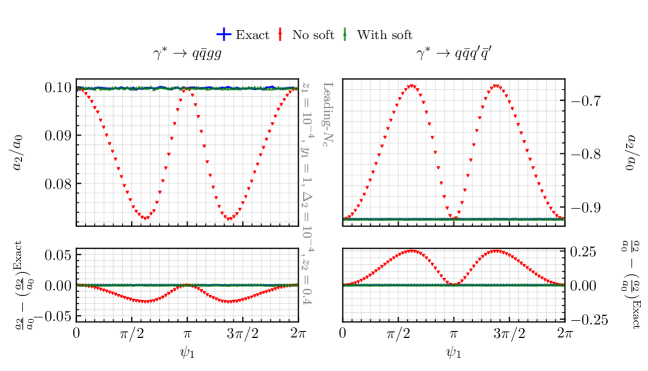
Figure 12: The same matrix element comparison as Fig. 3, but as a function of the intermediate gluon’s azimuthal angle $\psi_{1}$ instead of its rapidity $y_{1}$. The latter is fixed to $y_{1}=1$.

The branching amplitudes defined in Eqs. 2 and 7 involve spinor products, which must be evaluated numerically. Without loss of generality, the spinor product may be expressed as

$$S_{+}(p_{b},p_{c})=\frac{1}{\sqrt{p_{b}{\cdot}k_{0}}\sqrt{p_{c}{\cdot}k_{0}}}\bigg{[}(p_{c}{\cdot}k_{0})(p_{b}{\cdot}k_{1})-(p_{b}{\cdot}k_{0})(p_{c}{\cdot}k_{1})-i\epsilon_{\mu\nu\alpha\beta}k_{0}^{\mu}k_{1}^{\nu}p_{b}^{\alpha}p_{c}^{\beta}\bigg{]},$$ (27)

where $k_{0}$ and $k_{1}$ are arbitrary reference vectors which obey $k_{0}^{2}=k_{0}{\cdot}k_{1}=0$ and $k_{1}^{2}=-1$. In the evaluation of a complete, gauge-invariant squared scattering amplitude, any dependence on these reference directions must necessarily vanish. However, the branching amplitudes used in the Collins-Knowles algorithm only reproduce the full scattering amplitude in the relevant singular limits. Outside of this limit, a spurious dependence remains. In particular, in Ref. Karlberg:2021kwr it was shown that this dependence indeed vanishes in the collinear limit, but in that implementation it remains in the soft limit. Furthermore, because a definite choice must be made, this effect depends on the event orientation.

This issue is illustrated in Fig. 12, where the second-order matrix element comparison of Fig. 3 is repeated, but now as a function of $\psi_{1}$, the azimuth of the soft gluon emission, instead of $y_{1}$ which is fixed to $y_{1}=1$. As explained, without soft corrections the result depends on $\psi_{1}$, only reproducing the soft matrix element for the specific values $\psi_{1}=\{0,\pi,2\pi\}$. When soft corrections are instead enabled, the Collins-Knowles algorithm reproduces the soft matrix element for all values of $\psi_{1}$.

References

- (1) M. Dasgupta, F. A. Dreyer, K. Hamilton, P. F. Monni and G. P. Salam, Logarithmic accuracy of parton showers: a fixed-order study, JHEP 09 (2018) 033, [1805.09327].
- (2) M. Dasgupta, F. A. Dreyer, K. Hamilton, P. F. Monni, G. P. Salam and G. Soyez, Parton showers beyond leading logarithmic accuracy, Phys. Rev. Lett. 125 (2020) 052002, [2002.11114].
- (3) K. Hamilton, R. Medves, G. P. Salam, L. Scyboz and G. Soyez, Colour and logarithmic accuracy in final-state parton showers, JHEP 03 (2021) 041, [2011.10054].
- (4) A. Karlberg, G. P. Salam, L. Scyboz and R. Verheyen, Spin correlations in final-state parton showers and jet observables, Eur. Phys. J. C 81 (2021) 681, [2103.16526].
- (5) J. R. Forshaw, J. Holguin and S. Plätzer, Building a consistent parton shower, JHEP 09 (2020) 014, [2003.06400].
- (6) J. Holguin, J. R. Forshaw and S. Plätzer, Improvements on dipole shower colour, Eur. Phys. J. C 81 (2021) 364, [2011.15087].
- (7) Z. Nagy and D. E. Soper, Summations of large logarithms by parton showers, 2011.04773.
- (8) Z. Nagy and D. E. Soper, Summations by parton showers of large logarithms in electron-positron annihilation, 2011.04777.
- (9) B. Andersson, G. Gustafson, L. Lonnblad and U. Pettersson, Coherence Effects in Deep Inelastic Scattering, Z. Phys. C43 (1989) 625.
- (10) A. J. Larkoski, I. Moult and B. Nachman, Jet Substructure at the Large Hadron Collider: A Review of Recent Advances in Theory and Machine Learning, Phys. Rept. 841 (2020) 1–63, [1709.04464].
- (11) B. R. Webber, Monte Carlo Simulation of Hard Hadronic Processes, Ann. Rev. Nucl. Part. Sci. 36 (1986) 253–286.
- (12) J. C. Collins, Spin Correlations in Monte Carlo Event Generators, Nucl. Phys. B304 (1988) 794–804.
- (13) I. Knowles, Angular Correlations in QCD, Nucl. Phys. B 304 (1988) 767–793.
- (14) Z. Nagy and D. E. Soper, Parton showers with quantum interference, JHEP 09 (2007) 114, [0706.0017].
- (15) Z. Nagy and D. E. Soper, Parton showers with quantum interference: Leading color, with spin, JHEP 07 (2008) 025, [0805.0216].
- (16) J. R. Forshaw, J. Holguin and S. Plätzer, Parton branching at amplitude level, JHEP 08 (2019) 145, [1905.08686].
- (17) G. Corcella, I. G. Knowles, G. Marchesini, S. Moretti, K. Odagiri, P. Richardson et al., HERWIG 6: An Event generator for hadron emission reactions with interfering gluons (including supersymmetric processes), JHEP 01 (2001) 010, [hep-ph/0011363].
- (18) M. Bahr et al., Herwig++ Physics and Manual, Eur. Phys. J. C58 (2008) 639–707, [0803.0883].
- (19) J. Bellm et al., Herwig 7.0/Herwig++ 3.0 release note, Eur. Phys. J. C76 (2016) 196, [1512.01178].
- (20) P. Richardson and S. Webster, Spin Correlations in Parton Shower Simulations, Eur. Phys. J. C80 (2020) 83, [1807.01955].
- (21) S. J. Webster, Improved Monte Carlo Simulations of Massive Quarks. PhD thesis, Durham U., 2019.
- (22) R. Kleiss and W. Stirling, Spinor Techniques for Calculating p anti-p — W+- / Z0 + Jets, Nucl. Phys. B 262 (1985) 235–262.
- (23) A. Bassetto, M. Ciafaloni and G. Marchesini, Jet Structure and Infrared Sensitive Quantities in Perturbative QCD, Phys. Rept. 100 (1983) 201–272.
- (24) F. A. Berends and W. T. Giele, Recursive Calculations for Processes with n Gluons, Nucl. Phys. B 306 (1988) 759–808.
- (25) R. Mertig, M. Böhm and A. Denner, Feyn calc - computer-algebraic calculation of feynman amplitudes, Computer Physics Communications 64 (1991) 345–359.
- (26) V. Shtabovenko, R. Mertig and F. Orellana, New Developments in FeynCalc 9.0, Comput. Phys. Commun. 207 (2016) 432–444, [1601.01167].
- (27) V. Shtabovenko, R. Mertig and F. Orellana, FeynCalc 9.3: New features and improvements, Comput. Phys. Commun. 256 (2020) 107478, [2001.04407].
- (28) M. Heller and A. von Manteuffel, MultivariateApart: Generalized Partial Fractions, 2101.08283.
- (29) Wolfram Research, Inc., “Mathematica, Version 12.3.1.” https://www.wolfram.com, Champaign, IL, 2021.
- (30) Z. Nagy and Z. Trocsanyi, Next-to-leading order calculation of four jet observables in electron positron annihilation, Phys. Rev. D 59 (1999) 014020, [hep-ph/9806317].
- (31) S. D. Badger, E. W. N. Glover and V. V. Khoze, Recursion relations for gauge theory amplitudes with massive vector bosons and fermions, JHEP 01 (2006) 066, [hep-th/0507161].
- (32) S. Catani and M. Grazzini, Infrared factorization of tree level QCD amplitudes at the next-to-next-to-leading order and beyond, Nucl. Phys. B570 (2000) 287–325, [hep-ph/9908523].
- (33) Y. L. Dokshitzer, G. D. Leder, S. Moretti and B. R. Webber, Better jet clustering algorithms, JHEP 08 (1997) 001, [hep-ph/9707323].
- (34) M. Wobisch and T. Wengler, Hadronization corrections to jet cross-sections in deep inelastic scattering, in Workshop on Monte Carlo Generators for HERA Physics (Plenary Starting Meeting), pp. 270–279, 4, 1998. hep-ph/9907280.
- (35) M. Cacciari, G. P. Salam and G. Soyez, FastJet User Manual, Eur. Phys. J. C72 (2012) 1896, [1111.6097].
- (36) F. A. Dreyer, G. P. Salam and G. Soyez, The Lund Jet Plane, JHEP 12 (2018) 064, [1807.04758].
- (37) M. Dasgupta, F. Dreyer, G. P. Salam and G. Soyez, Small-radius jets to all orders in QCD, JHEP 04 (2015) 039, [1411.5182].
- (38) M. Dasgupta, F. A. Dreyer, G. P. Salam and G. Soyez, Inclusive jet spectrum for small-radius jets, JHEP 06 (2016) 057, [1602.01110].
- (39) A. Banfi, G. P. Salam and G. Zanderighi, Infrared safe definition of jet flavor, Eur. Phys. J. C 47 (2006) 113–124, [hep-ph/0601139].
- (40) S. Catani, Y. L. Dokshitzer, M. Olsson, G. Turnock and B. R. Webber, New clustering algorithm for multi - jet cross-sections in annihilation, Phys. Lett. B269 (1991) 432–438.
- (41) H. Chen, I. Moult and H. X. Zhu, Quantum Interference in Jet Substructure from Spinning Gluons, Phys. Rev. Lett. 126 (2021) 112003, [2011.02492].
- (42) L. Gellersen, S. Höche and S. Prestel, Disentangling soft and collinear effects in QCD parton showers, 2110.05964.
- (43) S. Platzer and M. Sjodahl, Subleading improved Parton Showers, JHEP 07 (2012) 042, [1201.0260].
- (44) Z. Nagy and D. E. Soper, Parton shower evolution with subleading color, JHEP 06 (2012) 044, [1202.4496].
- (45) Z. Nagy and D. E. Soper, Effects of subleading color in a parton shower, JHEP 07 (2015) 119, [1501.00778].
- (46) S. Plaetzer, M. Sjodahl and J. Thorén, Color matrix element corrections for parton showers, JHEP 11 (2018) 009, [1808.00332].
- (47) Z. Nagy and D. E. Soper, Parton showers with more exact color evolution, Phys. Rev. D 99 (2019) 054009, [1902.02105].
- (48) M. De Angelis, J. R. Forshaw and S. Plätzer, Resummation and Simulation of Soft Gluon Effects beyond Leading Color, Phys. Rev. Lett. 126 (2021) 112001, [2007.09648].
- (49) S. Höche and D. Reichelt, Numerical resummation at subleading color in the strongly ordered soft gluon limit, Phys. Rev. D 104 (2021) 034006, [2001.11492].
- (50) J. Holguin, J. R. Forshaw and S. Plätzer, Comments on a new ‘full colour’ parton shower, 2003.06399.