When Does Contrastive Learning Preserve
Adversarial Robustness from
Pretraining to Finetuning?

Abstract

Contrastive learning (CL) can learn generalizable feature representations and achieve state-of-the-art performance of downstream tasks by finetuning a linear classifier on top of it. However, as adversarial robustness becomes vital in image classification, it remains unclear whether or not CL is able to preserve robustness to downstream tasks. The main challenge is that in the ‘self-supervised pretraining + supervised finetuning’ paradigm, adversarial robustness is easily forgotten due to a learning task mismatch from pretraining to finetuning. We call such challenge ‘cross-task robustness transferability’. To address the above problem, in this paper we revisit and advance CL principles through the lens of robustness enhancement. We show that (1) the design of contrastive views matters: High-frequency components of images are beneficial to improving model robustness; (2) Augmenting CL with pseudo-supervision stimulus (e.g., resorting to feature clustering) helps preserve robustness without forgetting. Equipped with our new designs, we propose AdvCL, a novel adversarial contrastive pretraining framework. We show that AdvCL is able to enhance cross-task robustness transferability without loss of model accuracy and finetuning efficiency. With a thorough experimental study, we demonstrate that AdvCL outperforms the state-of-the-art self-supervised robust learning methods across multiple datasets (CIFAR-10, CIFAR-100 and STL-10) and finetuning schemes (linear evaluation and full model finetuning). Code is available at https://github.com/LijieFan/AdvCL.

1 Introduction

Image classification has been revolutionized by convolutional neural networks (CNNs). In spite of CNNs’ generalization power, the lack of adversarial robustness has shown to be a main weakness that gives rise to security concerns in high-stakes applications when CNNs are applied, e.g., face recognition, medical image classification, surveillance, and autonomous driving [1, 2, 3, 4, 5]. The brittleness of CNNs can be easily manifested by generating tiny input perturbations to completely alter the models’ decision. Such input perturbations and corresponding perturbed inputs are referred to as adversarial perturbations and adversarial examples (or attacks), respectively [6, 7, 8, 9, 10].

One of the most powerful defensive schemes against adversarial attacks is adversarial training (AT) [11], built upon a two-player game in which an ‘attacker’ crafts input perturbations to maximize the training objective for worst-case robustness, and a ‘defender’ minimizes the maximum loss for an improved robust model against these attacks. However, AT and its many variants using min-max optimization [12, 13, 14, 15, 16, 17, 18, 19, 20, 21] were restricted to supervised learning as true labels of training data are required for both supervised classifier and attack generator (that ensures misclassification). The recent work [22, 23, 24] demonstrated that with a properly-designed attacker’s objective, AT-type defenses can be generalized to the semi-supervised setting, and showed that the incorporation of additional unlabeled data could further improve adversarial robustness in image classification. Such an extension from supervised to semi-supervised defenses further inspires us to ask whether there exist unsupervised defenses that can eliminate the prerequisite of labeled data but improve model robustness.

Some very recent literature [25, 26, 27, 28, 29] started tackling the problem of adversarial defense through the lens of self-supervised learning. Examples include augmenting a supervised task with an unsupervised ‘pretext’ task for which ground-truth label is available for ‘free’ [25, 26], or robustifying unsupervised representation learning based only on a pretext task and then finetuning the learned representations over downstream supervised tasks [27, 28, 29]. The latter scenario is of primary interest to us as a defense can then be performed at the pretraining stage without needing any label information. Meanwhile, self-supervised contrastive learning (CL) has been outstandingly successful in the field of representation learning: It can surpass a supervised learning counterpart on downstream image classification tasks in standard accuracy [30, 31, 32, 33, 34]. Different from conventional self-supervised learning methods [35], CL, e.g., SimCLR [30], enforces instance discrimination by exploring multiple views of the same data and treating every instance under a specific view as a class of its own [36].

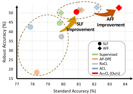
Figure 1: Summary of performance for various robust pretraining methods on CIFAR-10. The covered baseline methods include AP-DPE [26], RoCL [28], ACL [27] and supervised adversarial training (AT) [11]. Upper-right indicates better performance with respect to (w.r.t.) standard accuracy and robust accuracy (under PGD attack with $20$ steps and $8/255$ $\ell_{\infty}$-norm perturbation strength). Different colors represent different pretraining methods, and different shapes represent different finetuning settings. Circles (⚫) indicates Standard Linear Finetuning (SLF), and Diamonds (◆) indicates Adversarial Full Finetuning (AFF). Our method (AdvCL, red circle/diamond) has the best performance across finetuning settings. Similar improvement could be observed under Auto-Attacks, and we provide the visualization in the appendix.

The most relevant work to ours is [27, 28], which integrated adversarial training with CL. However, the achieved adversarial robustness at downstream tasks largely relies on the use of advanced finetuning techniques, either adversarial full finetuning [27] or adversarial linear finetuning [28]. Different from [27, 28], we ask:

(Q) How to accomplish robustness enhancement using CL without losing its finetuning efficiency, e.g., via a standard linear finetuner?

Our work attempts to make a rigorous and comprehensive study on addressing the above question. We find that self-supervised learning (including the state-of-the-art CL) suffers a new robustness challenge that we call ‘cross-task robustness transferability’, which was largely overlooked in the previous work. That is, there exists a task mismatch from pretraining to finetuning (e.g., from CL to supervised classification) so that adversarial robustness is not able to transfer across tasks even if pretraining datasets and finetuning datasets are drawn from the same distribution. Different from supervised/semi-supervised learning, this is a characteristic behavior of self-supervision when being adapted to robust learning. As shown in Figure 1, our work advances CL in the adversarial context and the proposed method outperforms all state-of-the-art baseline methods, leading to a substantial improvement in both robust accuracy and standard accuracy using either the lightweight standard linear finetuning or end-to-end adversarial full finetuning.

Contributions

Our main contributions are summarized below.

❶ We propose AdvCL, a unified adversarial CL framework, and propose to use original adversarial examples and high-frequency data components to create robustness-aware and generalization-aware views of unlabeled data.

❷ We propose to generate proper pseudo-supervision stimulus for AdvCL to improve cross-task robustness transferability. Different from existing self-supervised defenses aided with labeled data [27], we generate pseudo-labels of unlabeled data based on their clustering information.

❸ We conduct a thorough experimental study and show that AdvCL achieves state-of-the-art robust accuracies under both PGD attacks [11] and Auto-Attacks [37] using only standard linear finetuning. For example, in the case of Auto-Attack (the most powerful threat model) with $8/255$ $\ell_{\infty}$-norm perturbation strength under ResNet-18, we achieve $3.44\%$ and $3.45\%$ robustness improvement on CIFAR-10 and CIFAR-100 over existing self-supervised methods. We also justify the effectiveness of AdvCL in different attack setups, dataset transferring, model explanation, and loss landscape smoothness.

2 Background & Related Work

Self-Supervised Learning Early approaches for unsupervised representation learning leverages handcrafted tasks, like prediction rotation [38] and solving the Jigsaw puzzle [39, 40], geometry prediction [41] and Selfie [42]. Recently contrastive learning (CL) [30, 33, 34, 43, 44, 45] and its variants [31, 32, 36, 46] have demonstrated superior abilities in learning generalizable features in an unsupervised manner. The main idea behind CL is to self-create positive samples of the same image from aggressive viewpoints, and then acquire data representations by maximizing agreement between positives while contrasts with negatives.

In what follows, we elaborate on the formulation of SimCLR [30], one of the most commonly-used CL frameworks, which this paper will focus on. To be concrete, let $\mathcal{X}=\{x_{1},x_{2},...,x_{n}\}$ denote an unlabeled source dataset, SimCLR offers a learned feature encoder $f_{\theta}$ to generate expressive deep representations of the data. To train $f_{\boldsymbol{\theta}}$, each input $x\in\mathcal{X}$ will be transformed into two views $(\tau_{1}(x),\tau_{2}(x))$ and labels them as a positive pair. Here transformation operations $\tau_{1}$ and $\tau_{2}$ are randomly sampled from a pre-defined transformation set $\mathcal{T}$, which includes, e.g., random cropping and resizing, color jittering, rotation, and cutout. The positive pair is then fed in the feature encoder $f_{\theta}$ with a projection head $g$ to acquire projected features, i.e., $z_{i}=g\circ f_{\theta}(\tau_{i}(x))$ for $j\in\{1,2\}$. NT-Xent loss (i.e., the normalized temperature-scaled cross-entropy loss) is then applied to optimizing $f_{\theta}$, where the distance of projected positive features $(z_{1},z_{2})$ is minimized for each input $x$. SimCLR follows the ‘self-supervised pretraining + supervised finetuning’ paradigm. That is, once $f_{\theta}$ is trained, a downstream supervised classification task can be handled by just finetuning a linear classifier $\phi$ over the fixed encoder $f_{\theta}$, leading to the eventual classification network $\phi\circ f_{\theta}$.

Adversarial Training (AT) Deep neural networks are vulnerable to adversarial attacks. Various approaches have been proposed to enhance the model robustness. Given a classification model $\theta$, AT [11] is one of the most powerful robust training methods against adversarial attacks. Different from standard training over normal data $(x,y)\in\mathcal{D}$ (with feature $x$ and label $y$ in dataset $\mathcal{D}$), AT adopts a min-max training recipe, where the worst-case training loss is minimized over the adversarially perturbed data $(x+\delta,y)$. Here $\delta$ denotes the input perturbation variable to be maximized for the worst-case training objective. The supervised AT is then formally given by

$$\min_{\theta}\mathbb{E}_{{(x,y)}\in{D}}\max_{\|\delta\|_{\infty}\leq\epsilon}\ell(x+\delta,y;\theta),$$ (1)

where $\ell$ denotes the supervised training objective, e.g., cross-entropy (CE) loss. There have been many variants of AT [19, 20, 21, 47, 48, 49, 50, 22, 23, 24, 25] established for supervised/semi-supervised learning.

Self-supervision enabled AT

Several recent works [26, 27, 28, 29] started to study how to improve model robustness using self-supervised AT. Their idea is to apply AT (1) to a self-supervised pretraining task, e.g., SimCLR in [27, 28], such that the learned feature encoder $f_{\theta}$ renders robust data representations. However, different from our work, the existing ones lack a systematic study on when and how self-supervised robust pretraining can preserve robustness to downstream tasks without sacrificing the efficiency of lightweight finetuning. For example, the prior work [26, 27] suggested adversarial full finetuning, where pretrained model is used as a weight initialization in finetuning downstream tasks. Yet, it requests the finetuner to update all of the weights of the pretrained model, and thus makes the advantage of self-supervised robust pretraining less significant. A more practical scenario is linear finetuning: One freezes the pretrained feature encoder for the downstream task and only partially finetunes a linear prediction head. The work [28] evaluated the performance of linear fintuning but observed a relatively large performance gap between the standard linear finetuning and adversarial linear finetuning; see more comparisons in Figure 1. Therefore, the problem–how to enhance robustness transferability from pretraining to linear finetuning–remains unexplored.

3 Problem Statement

In this section, we present the problem of our interest, together with its setup.

Robust pretraining + linear finetuning.

We aim to develop robustness enhancement solutions by fully exploiting and exploring the power of CL at the pretraining phase, so that the resulting robust feature representations can seamlessly be used to generate robust predictions of downstream tasks using just a lightweight finetuning scheme. With the aid of AT (1), we formulate the ‘robust pretraining + linear finetuning’ problem below:

$$\text{Pretraining:}~{}\displaystyle\min_{\theta}\mathbb{E}_{{x}\in\mathcal{X}}\max_{\|\delta\|_{\infty}\leq\epsilon}\ell_{\mathrm{pre}}(x+\delta,x;\theta)$$ (2)

$$\text{Finetuning:}~{}\displaystyle\min_{\theta_{\mathrm{c}}}\mathbb{E}_{{(x,y)}\in{\mathcal{D}}}\,\ell_{\mathrm{CE}}(\phi_{\theta_{\mathrm{c}}}\circ f_{\theta}(x),y),$$ (3)

where $\ell_{\mathrm{pre}}$ denotes a properly-designed robustness- and generalization-aware CL loss (see Sec. 4) given as a function of the adversarial example $(x+\delta)$, original example $x$ and feature encoder parameters $\theta$. In (2), $\phi_{\theta_{\mathrm{c}}}\circ f_{\theta}$ denotes the classifier by equipping the linear prediction head $\phi_{\theta_{\mathrm{c}}}$ (with parameters $\theta_{\mathrm{c}}$ to be designed) on top of the fixed feature encoder $f_{\theta}$, and $\ell_{\mathrm{CE}}$ denotes the supervised CE loss over the target dataset $\mathcal{D}$. Note that besides the standard linear finetuning (3), one can also modify (3) using the worst-case CE loss for adversarial linear/full finetuning [27, 28]. We do not consider standard full finetuning in the paper since tuning the full network weights with standard cross-entropy loss is not possible for the model to preserve robustness [26].

Cross-task robustness transferability.

Different from supervised/semi-supervised learning, self-supervision enables robust pretraining over unlabeled source data. In the meantime, it also imposes a new challenge that we call ‘cross-task robustness transferability’: At the pretraining stage, a feature encoder is learned over a ‘pretext’ task for which ground-truth is available for free, while finetuning is typically carried out on a new downstream task. Spurred by the above, we ask the following questions:

• Will CL improve adversarial robustness using just standard linear finetuning?

• What are the principles that CL should follow to preserve robustness across tasks?

• What are the insights can we acquire from self-supervised robust representation learning?

4 Proposed Approach: Adversarial Contrastive Learning (AdvCL)

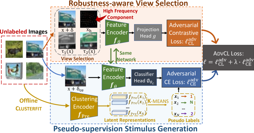
Figure 2: The overall pipeline of AdvCL. It mainly has two ingredients: robustness-aware view selection (orange box) and pseudo-supervision stimulus generation (blue box). The view selection mechanism is advanced by high frequency components, and the supervision stimulus is created by generating pseudo labels for each image through ClusterFit. The pseudo label (in yellow color) can be created in an offline manner and will not increase the computation overhead.

In this section, we develop a new adversarial CL framework, AdvCL, which includes two main components, robustness-aware view selection and pseudo-supervision stimulus generation. In particular, we advance the view selection mechanism by taking into account proper frequency-based data transformations that are beneficial to robust representation learning and pretraining generalization ability. Furthermore, we propose to design and integrate proper supervision stimulus into AdvCL so as to improve the cross-task robustness transferability since robust representations learned from self-supervision may lack the class-discriminative ability required for robust predictions on downstream tasks. We provide an overview of AdvCL in Figure 2.

4.1 View selection mechanism

In contrast to standard CL, we propose two additional contrastive views: the adversarial view and the frequency view, respectively.

Multi-view CL loss

Prior to defining new views, we first review the NT-Xent loss and its multi-view version used in CL. Following notations defined in Sec. 2, the contrastive loss with respect to (w.r.t.) a positive pair $(\tau_{1}(x),\tau_{2}(x))$ of each (unlabeled) data $x$ is given by

$$\ell_{\mathrm{CL}}(\tau_{1}(x),\tau_{2}(x))=-\sum_{i=1}^{2}\sum_{j\in\mathcal{P}(i)}\log\frac{\exp\big{(}\text{sim}(z_{i},z_{j})/t\big{)}}{\displaystyle\sum_{k\in\mathcal{N}(i)}\exp\big{(}\text{sim}(z_{i},z_{k})/t\big{)}},$$ (4)

where recall that $z_{i}=g\circ f(\tau_{i}(x))$ is the projected feature under the $i$th view, $\mathcal{P}(i)$ is the set of positive views except $i$ (e.g., $\mathcal{P}(i)=\{2\}$ if $i=1$), $\mathcal{N}(i)$ denotes the set of augmented batch data except the point $\tau_{i}(x)$, the cardinality of $\mathcal{N}(i)$ is $(2b-1)$ (for a data batch of size $b$ under $2$ views), $\text{sim}(z_{i1},z_{i2})$ denotes the cosine similarity between representations from two views of the same data, $\mathrm{exp}$ denotes exponential function, $\mathrm{sim}(\cdot,\cdot)$ is the cosine similarity between two points, and $t>0$ is a temperature parameter. The two-view CL objective can be further extend to the multi-view contrastive loss [51]

$$\ell_{\mathrm{CL}}(\tau_{1}(x),\tau_{2}(x),\ldots,\tau_{m}(x))=-\sum_{i=1}^{m}\sum_{j\in\mathcal{P}(i)}\log\frac{\exp\big{(}\text{sim}(z_{i},z_{j})/t\big{)}}{\displaystyle\sum_{k\in\mathcal{N}(i)}\exp\big{(}\text{sim}(z_{i},z_{k})/t\big{)}},$$ (5)

where $\mathcal{P}(i)=[m]/\{i\}$ denotes the $m$ positive views except $i$, $[m]$ denotes the integer set $\{1,2,\ldots,m\}$, and $\mathcal{N}(i)$, with cardinality $(bm-1)$, denotes the set of $m$-view augmented $b$ batch samples except the point $\tau_{i}(x)$.

Contrastive view from adversarial example

Existing methods proposed in [27, 28, 29] can be explained based on (4): An adversarial perturbation $\boldsymbol{\delta}$ w.r.t. each view of a sample $x$ is generated by maximizing the contrastive loss:

$$\delta_{1}^{*},\delta_{2}^{*}=\displaystyle\operatorname*{\operatorname*{argmax}}_{\|\delta_{i}\|_{\infty}\leq\epsilon}\ell_{\mathrm{CL}}(\tau_{1}(x)+\delta_{1},\tau_{2}(x)+\delta_{2}).$$ (6)

A solution to problem (6) eventually yields a paired perturbation view $(\tau_{1}(x)+\delta_{1}^{*},\tau_{2}(x)+\delta_{2}^{*})$. However, the definition of adversarial view (6) used in [27, 28, 29] may not be proper. First, standard CL commonly uses aggressive data transformation that treats small portions of images as positive samples of the full image [36]. Despite its benefit to promoting generalization, crafting perturbations over such aggressive data transformations may not be suitable for defending adversarial attacks applied to full images in the adversarial context. Thus, a new adversarial view built upon $x$ rather than $\tau_{i}(x)$ is desired. Second, the contrastive loss (4) is only restricted to two views of the same data. As will be evident later, the multi-view contrastive loss is also needed when taking into account multiple robustness-promoting views. Spurred by above, we define the adversarial view over $x$, without modifying the existing data augmentations $(\tau_{1}(x),\tau_{2}(x))$. This leads to the following adversarial perturbation generator by maximizing a $3$-view contrastive loss

$$\delta^{*}=\displaystyle\operatorname*{\operatorname*{argmax}}_{\|\delta\|\leq\epsilon}\ell_{\mathrm{CL}}(\tau_{1}(x),\tau_{2}(x),x+\delta),$$ (7)

where $x+\delta^{*}$ is regarded as the third view of $x$.

Contrastive view from high-frequency component

Next, we use the high-frequency component (HFC) of data as another additional contrastive view. The rationale arises from the facts that 1) learning over HFC of data is a main cause of achieving superior generalization ability [52] and 2) an adversary typically concentrates on HFC when manipulating an example to fool model’s decision [53]. Let $\mathcal{F}$ and $\mathcal{F}^{-1}$ denote Fourier transformation and its inverse. An input image $x$ can then be decomposed into its HFC $x_{\mathrm{h}}$ and low-frequency component (LFC) $x_{\mathrm{l}}$:

$$x_{\mathrm{h}}=\mathcal{F}^{-1}(q_{\mathrm{h}}),\quad x_{\mathrm{l}}=\mathcal{F}^{-1}(q_{\mathrm{l}}),\quad[q_{\mathrm{h}},q_{\mathrm{l}}]=\mathcal{F}(x).$$ (8)

In (8), the distinction between $q_{\mathrm{h}}$ and $q_{\mathrm{l}}$ is made by a hard thresholding operation. Let $q(i,j)$ denote the $(i,j)$th element of $\mathcal{F}(x)$, and $c=(c_{1},c_{2})$ denote the centriod of the frequency spectrum. The components $q_{\mathrm{l}}$ and $q_{\mathrm{h}}$ in (8) are then generated by filtering out values according to the distance from $c$: $q_{h}(i,j)=\mathbbm{1}_{[d((i,j),(c_{1},c_{2}))\geq r]}\cdot q(i,j)$, and $q_{l}(i,j)=\mathbbm{1}_{[d((i,j),(c_{1},c_{2}))\leq r]}\cdot q(i,j)$, where $d(\cdot,\cdot)$ is the Euclidian distance between two spatial coordinates, $r$ is a pre-defined distance threshold ($r=8$ in all our experiments), and $\mathbbm{1}_{[.]}\in\{0,1\}$ is an indicator function which equals to $1$ if the condition within $[\cdot]$ is met and $0$ otherwise.

Robustness-aware contrastive learning objective

By incorporating the adversarial perturbation $\delta$ and disentangling HFC $x_{\mathrm{h}}$ from the original data $x$, we obtain a four-view contrastive loss (5) defined over $(\tau_{1}(x),\tau_{2}(x),x+\delta,x_{\mathrm{h}})$,

$$\ell_{\mathrm{CL}}^{\mathrm{adv}}(\theta;\mathcal{X})\mathrel{\mathop{:}}=\mathbb{E}_{{x}\in{\mathcal{X}}}\max_{\|\delta\|_{\infty}\leq\epsilon}\ell_{\mathrm{CL}}(\tau_{1}(x),\tau_{2}(x),x+\delta,x_{\mathrm{h}};\theta),$$ (9)

where recall that $\mathcal{X}$ denotes the unlabeled dataset, $\epsilon>0$ is a perturbation tolerance during training, and for clarity, the four-view contrastive loss (5) is explicitly expressed as a function of model parameters $\theta$. As will be evident latter, the eventual learning objective AdvCL will be built upon (9).

4.2 Supervision stimulus generation: AdvCL empowered by ClusterFit

On top of (9), we further improve the robustness transferability of learned representations by generating a proper supervision stimulus. Our rationale is that robust representation could lack the class-discriminative power required by robust classification as the former is acquired by optimizing an unsupervised contrastive loss while the latter is achieved by a supervised cross-entropy CE loss. However, there is no knowledge about supervised data during pretraining. In order to improve cross-task robustness transferability but without calling for supervision, we take advantage of ClusterFit [54], a pseudo-label generation method used in representation learning.

To be more concrete, let $f_{\mathrm{pre}}$ denote a pretrained representation network that can generate latent features of unlabeled data. Note that $f_{\mathrm{pre}}$ can be set available beforehand and trained over either supervised or unsupervised dataset $\mathcal{D}_{\mathrm{pre}}$, e.g., ImageNet using using CL in experiments. Given (normalized) pretrained data representations $\{f_{\mathrm{pre}}(x)\}_{x\in\mathcal{X}}$, ClusterFit uses $K$-means clustering to find $K$ data clusters of $\mathcal{X}$, and maps a cluster index $c$ to a pseudo-label, resulting in the pseudo-labeled dataset $\{(x,c)\in\hat{\mathcal{X}}\}$. By integrating ClusterFit with (9), the eventual training objective of AdvCL is then formed by

$$\min_{\theta}~{}\ell_{\mathrm{CL}}^{\mathrm{adv}}(\theta;\mathcal{X})+\lambda\min_{\theta,\theta_{\mathrm{c}}}~{}\underbrace{\mathbb{E}_{{(x,c)}\in{\hat{\mathcal{X}}}}\max_{\|\delta_{ce}\|_{\infty}\leq\epsilon}\ell_{\mathrm{CE}}(\phi_{\theta_{\mathrm{c}}}\circ f_{\theta}(x+\delta_{ce}),c)}_{\text{Pseudo-classification enabled AT regularization}},$$ (10)

where $\hat{\mathcal{X}}$ denotes the pseudo-labeled dataset of $\mathcal{X}$, $\phi_{\theta_{\mathrm{c}}}$ denotes a prediction head over $f_{\theta}$, and $\lambda>0$ is a regularization parameter that strikes a balance between adversarial contrastive training and pseudo-label stimulated AT. When the number of clusters $K$ is not known a priori, we extend (10) to an ensemble version over $n$ choices of cluster numbers $\{K_{1},\ldots,K_{n}\}$. Here each cluster number $K_{i}$ is paired with a unique linear classifier $\phi_{i}$ to obtain the supervised prediction $\phi_{i}\circ f$ (using cluster labels). The ensemble CE loss, given by the average of $n$ individual losses, is then used in (10). Our experiments show that the ensemble version usually leads to better generalization ability.

5 Experiments

In this section, we demonstrate the effectiveness of our proposed AdvCL from the following aspects: (1) Quantitative results, including cross-task robustness transferability, cross-dataset robustness transferability, and robustness against PGD attacks [11] and Auto-Attacks [37]; (2) Qualitative results, including representation t-SNE [55], feature inversion map visualization, and geometry of loss landscape; (3) Ablation studies of AdvCL, including finetuning schemes, view selection choices, and supervision stimulus variations.

Experiment setup

We consider three robustness evaluation metrics: (1) Auto-attack accuracy (AA), namely, classification accuracy over adversarially perturbed images via Auto-Attacks; (2) Robust accuracy (RA), namely, classification accuracy over adversarially perturbed images via PGD attacks; and (3) Standard accuracy (SA), namely, standard classification accuracy over benign images without perturbations. We use ResNet-18 for the encoder architecture of $f_{\boldsymbol{\theta}}$ in CL. Unless specified otherwise, we use $5$-step $\ell_{\infty}$ projected gradient descent (PGD) with $\epsilon=8/255$ to generate perturbations during pretraining, and use Auto-Attack and $20$-step $\ell_{\infty}$ PGD with $\epsilon=8/255$ to generate perturbations in computing AA and RA at test time. We will compare AdvCL with the CL-based adversarial pretraining baselines , ACL [27], RoCL [28], (non-CL) self-supervised adversarial learning baseline AP-DPE [26] and the supervised AT baseline [11].

Table 1: Cross-task performance of AdvCL (in dark gray color), compared with supervised (in white color) and self-supervised (in light gray color) baselines, in terms of AA, RA and SA on CIFAR-10 with ResNet-18. The pretrained models are evaluated under the standard linear finetuning (SLF) setting and the adversarial full finetuning (AFF) setting. The top performance is highlighted in bold.

Pretraining Method	Finetuning Method	CIFAR-10			CIFAR-100
		AA(%)	RA(%)	SA(%)	AA(%)	RA(%)	SA(%)
Supervised	Standard linear finetuning (SLF)	42.22	44.4	79.77	19.53	23.41	50.53
AP-DPE[26]		16.07	18.22	78.30	4.17	6.23	47.91
RoCL[28]		28.38	39.54	79.90	8.66	18.79	49.53
ACL[27]		39.13	42.87	77.88	16.33	20.97	47.51
AdvCL (ours)		42.57	50.45	80.85	19.78	27.67	48.34
Supervised	Adversarial full finetuning (AFF)	46.19	49.89	79.86	21.61	25.86	52.22
AP-DPE[26]		48.13	51.52	81.19	22.53	26.89	55.27
RoCL[28]		47.88	51.35	81.01	22.38	27.49	55.10
ACL[27]		49.27	52.82	82.19	23.63	29.38	56.61
AdvCL (ours)		49.77	52.77	83.62	24.72	28.73	56.77

5.1 Quantitative Results

Overall performance from pretraining to finetuning (across tasks)

In Table 1, we evaluate the robustness of a classifier (ResNet-18) finetuned over robust representations learned by different supervised/self-supervised pretraining approaches over CIFAR-10 and CIFAR-100. We focus on two representative finetuning schemes: the simplest standard linear finetuning (SLF) and the end-to-end adversarial full finetuning (AFF). As we can see, the proposed AdvCL method yields a substantial improvement over almost all baseline methods. Moreover, AdvCL improves robustness and standard accuracy simultaneously.

Table 2: Cross-dataset performance of AdvCL (dark gray color), compared with supervised (white color) and self-supervised (light gray) baselines, in AA, RA, SA, on STL-10 with ResNet-18.

Method	Fine- tuning	CIFAR-10 $\xrightarrow[]{}$ STL-10			CIFAR-100 $\xrightarrow[]{}$ STL-10
		AA(%)	RA(%)	SA(%)	AA(%)	RA(%)	SA(%)
Supervised	SLF	22.26	30.45	54.70	19.54	23.63	51.11
RoCL[28]		18.65	28.18	54.56	12.39	21.93	47.86
ACL[27]		25.29	31.80	55.81	21.75	26.32	45.91
AdvCL (ours)		25.74	35.80	63.73	20.86	30.35	50.71
Supervised	AFF	33.10	36.7	62.78	29.18	32.43	55.85
RoCL[28]		29.40	34.65	61.75	27.55	31.38	57.83
ACL[27]		32.50	35.93	62.65	28.68	32.41	57.16
AdvCL (ours)		34.70	37.78	63.52	30.51	33.70	61.56

Robustness transferability across datasets

In Table 2, we next evaluate the robustness transferability across different datasets, where $A\to B$ denotes the transferability from pretraining on dataset $A$ to finetuning on another dataset $B$ ($\neq A$) of representations learned by AdvCL. Here the pretraining setup is consistent with Table 1. We observe that AdvCL yields better robustness as well as standard accuracy than almost all baseline approaches under both SLF and AFF finetuning settings. In the case of CIFAR-100 $\xrightarrow[]{}$ STL-10, although AdvCL yields $0.89\%$ AA drop compared to ACL [27], it yields a much better SA with $4.8\%$ improvement.

Robustness evaluation vs. attack strength

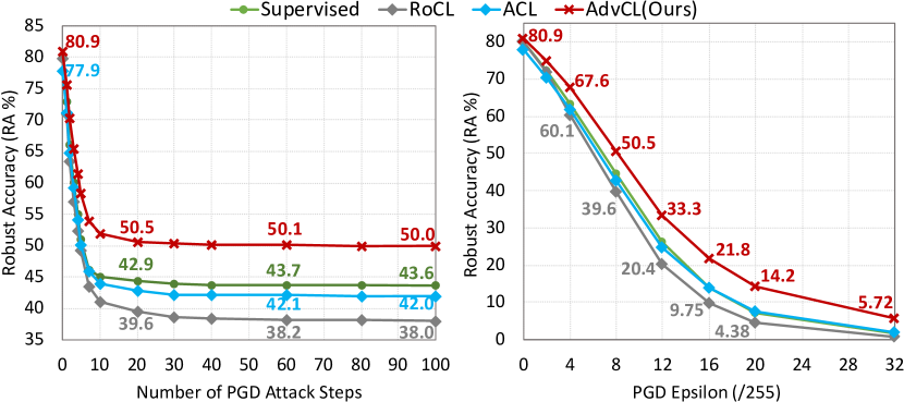
Figure 3: RA of AdvCL and baseline approaches under various PGD attacks. SLF is applied to the pretrained model.

It was shown in [56] that an adversarial defense that causes obfuscated gradients results in a false sense of model robustness. The issue of obfuscated gradients typically comes with two ‘side effects’: (a) The success rate of PGD attack ceases to be improved as the $\ell_{\infty}$-norm perturbation radius $\epsilon$ increases; (b) A larger number of PGD steps fails to generate stronger adversarial examples. Spurred by the above, Figure 3 shows the finetuning performance of AdvCL (using SLF) as a function of the perturbation size $\epsilon$ and the PGD step number. As we can see, AdvCL is consistently more robust than the baselines at all different PGD settings for a significant margin.

5.2 Qualitative Results

Class discrimination of learned representations

To further demonstrate the efficacy of AdvCL, Figure 4 visualizes the representations learned by self-supervision using t-SNE [55] on CIFAR-10. We color each point using its ground-truth label. The results show representations learned by AdvCL have a much clearer class boundary than those learned with baselines. This indicates that AdvCL makes an adversary difficult to successfully perturb an image, leading to a more robust prediction.

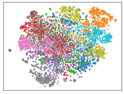
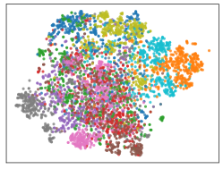
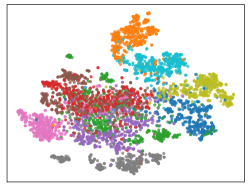
(a) RoCL [28]	(b) ACL [27]	(c) AdvCL (ours)

Figure 4: t-SNE visualization of representations learned with different self-supervised pretraining approaches. Our AdvCL gives a much clearer separation among classes than baseline approaches.

Seed Images AT RoCL ACL AdvCL

Figure 5: FIM visualization of neuron $502$ under CIFAR-10 using different robust training methods. Column $1$ contains different seed images to generate FIM. Columns 2-5 are FIMs using models trained with different approaches.

Visual interpretability of learned representations

Furthermore, we demonstrate the advantage of our proposals from the perspective of model explanation, characterized by feature inversion map (FIM) [57] of internal neurons’ response. The work [18, 58, 59] showed that model robustness offered by supervised AT and its variants enforces hidden neurons to learn perceptually-aligned data features through the lens of FIM. However, it remains unclear whether or not self-supervised robust pretraining is able to render explainable internal response. Following [57, 58], we acquire FIM of the $i$th component of representation vector by solving the optimization problem $x_{\mathrm{FIM}}=\min_{\Delta}[f_{\theta}(x_{0}+\Delta)]_{i}$, where $x_{0}$ is a randomly selected seed image, and $[\cdot]_{i}$ denotes the $i$th coordinate of a vector. Figure 5 shows that compared to other approaches, more similar texture-aligned features can be acquired from a neuron’s feature representation of the network trained with our method regardless of the choice of seed images.

Flatter loss landscape implies better transferability

It has been shown in [60] that the flatness of loss landscape is a good indicator for superb transferability in the pretraining + finetuning paradigm. Motivated by that, Figure 6 presents the adversarial loss landscape of AdvCL and other self-supervised pretraining approaches under SLF, where the loss landscape is drawn using the method in [61]. Note that instead of standard CE loss, we visualize the adversarial loss w.r.t. model weights. As we can see, the loss for AdvCL has a much flatter landscape around the local optima, whereas the losses for the other approaches change more rapidly. This justifies that our proposal has a better robustness transferability than baseline approaches.

Table 3: Performance (RA and SA) of AdvCL (in dark gray color) and baseline approaches on CIFAR-10, under different linear finetuning strategies: SLF and adversarial linear finetuning (ALF). Method SLF ALF RA(%) SA(%) RA(%) SA(%) Supervised 44.40 79.77 46.75 79.06 RoCL[28] 39.54 79.90 43.11 77.33 ACL[27] 42.87 77.88 45.40 77.71 AdvCL(ours) 50.45 80.85 52.01 79.39 Table 4: Performance (RA and SA) of AdvCL using different contrastive views setups. ResNet-18 is the backbone network, CIFAR-10 is the dataset, and SLF is used for classification. Contrastive Views RA(%) SA(%) $\tau_{1}(x)+\delta_{1},\tau_{2}(x)$ 42.12 77.07 $\tau_{1}(x)+\delta_{1},\tau_{2}(x)+\delta_{2}$ 42.48 73.12 $\tau_{1}(x)+\delta_{1},\tau_{2}(x)+\delta_{2},\tau_{1}(x),\tau_{2}(x)$ 43.51 74.22 ${x+\delta,\tau_{1}(x),\tau_{2}(x)}$ 50.19 80.17 $x+\delta,\tau_{1}(x),\tau_{2}(x),x_{\mathrm{l}}$ 49.51 79.83 $x+\delta,\tau_{1}(x),\tau_{2}(x),x_{\mathrm{l}},x_{\mathrm{h}}$ 50.03 80.14 ${x+\delta,\tau_{1}(x),\tau_{2}(x),x_{\mathrm{h}}}$ 50.45 80.85

Table 5: Performance (RA and SA) of AdvCL using various pretrained models $f_{\mathrm{pre}}$ and cluster numbers $K$ in ClusterFit, as well as the baseline w/o using ClusterFit. The setup of $f_{\mathrm{pre}}$ is specified by the training method (supervised training or SimCLR) and training dataset (ImageNet or CIFAR-10). AdvCL is implemented using unlabeled data from CIFAR-10 under ResNet-18, together with SLF over the acquired feature encoder for supervised CIFAR-10 classification. $f_{\mathrm{pre}}$ setup: (dataset, training) Cluster number $K$ RA (%) SA (%) N/A w/o ClusterFit 48.89 77.73 (CIFAR-10, SimCLR) 10 50.10 80.34 100 49.21 79.52 (ImageNet, supervised) 10 50.16 78.27 100 49.27 78.08 (ImageNet, SimCLR) 2 50.09 79.72 10 50.12 79.93 50 49.27 79.55 100 49.16 79.07 500 49.03 78.96 Ensemble 50.45 80.85

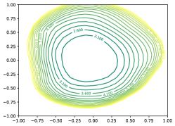
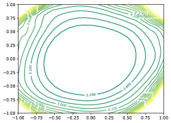
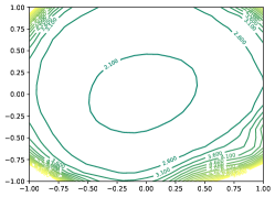
(a) RoCL [28]	(b) ACL [27]	(c) AdvCL(ours)

Figure 6: Visualization of adversarial loss landscape w.r.t. model weights using different self-supervised pretraining methods. AdvCL gives a much flatter landscape than the other baselines.

5.3 Ablation studies

Linear finetuning types

We first study the robustness difference when different linear finetuning strategies: Standard linear finetuning (SLF) and Adversarial linear finetuning (ALF) are applied. Table 5 shows the performance of models trained with different pretraining methods. As we can see, our AdvCL achieves the best performance under both linear finetuning settings and outperforms baseline approaches in a large margin. We also note the performance gap between SLF and ALF induced by our proposal AdvCL is much smaller than other approaches, and AdvCL with SLF achieves much better performance than baseline approaches with ALF. This indicates that the representations learned by AdvCL is already sufficient to yield satisfactory robustness.

View selection setup

We illustrate how different choices of contrastive views influence the robustness performance of AdvCL in Table 5. The first 4 rows study the effect of different types of adversarial examples in contrastive views, and our proposed 3-view contrastive loss (7) significantly outperforms the other baselines, as shown in row 4. The rows in gray show the performance of further exploring different image frequency components (8) as different contrastive views. It is clear that the use of HFC leads to the best overall performance, as shown in the last row.

Supervision stimulus setup

We further study the performance of AdvCL using different supervision stimulus. Specifically, we vary the pretrained model for $f_{\mathrm{pre}}$ and pseudo cluster number $K$ when training AdvCL and summarize the results in Table 5. The results demonstrate that adding the supervision stimulus could boost the performance of AdvCL. We also observe that the best result comes from $f_{\mathrm{pre}}$ pretrained on Imagenet using SimCLR. This is because such representations could generalize better. Moreover, the ensemble scheme over pseudo label categories $K\in\{2,10,50,100,500\}$ yields better results than using a single number of clusters. The ensemble scheme also makes AdvCL less sensitive to the actual number of labels for the training dataset.

6 Conclusion

In this paper, we study the good practices in making contrastive learning robust to adversarial examples. We show that adding perturbations to original images and high-frequency components are two beneficial factors. We further show that proper supervision stimulus could improve model robustness. Our proposed approaches can achieve state-of-the-art robust accuracy as well as standard accuracy using just standard linear finetuning. Extensive experiments involving quantitative and qualitative analysis have also been made not only to demonstrate the effectiveness of our proposals but also to rationalize why it yields superior performance. Future works could be done to improve the scalability of our proposed self-supervised pretraining approach to very large datasets and models to further boost robust transferabilty across datasets.

This supplementary material provides additional implementation details and experimental results.

A. Discussion and Broader Impact

In this paper we propose a powerful framework, AdvCL, which could preserve robustness from pretraining to finetuning, and we empircally show that the light-weight standard linear finetuning is already sufficient to give us comparable performance to the computational-expensive adversarial full finetuning. We don’t think our work would have negative societal impacts. The potential broader impact of our work is that, with the help of our proposed pretraining design paradigm, neural models could preserve adversarial robustness using lightweight linear finetuners, which could be deployed to embodied systems and can make real-time applications more secure and trustworthy on mobile devices.

B. Implementation Details

Pretraining Details

We list implementation details for AdvCL pretraining in this section. We use SGD optimizer with batch size=$512$, initial learning rate=$0.5$, momentum=$0.9$, and weight decay=$0.0001$ to train the network for $1000$ epochs. We use cosine learning rate decay during training, and we use the first $10$ epochs to warm-up learning rate from $0.01$ to $0.5$. The temperature parameter in contrastive loss $\ell_{\mathrm{CL}}$ is set to $t=0.5$, and the regularization parameter for the cross-entropy term with pseudo labels in Eq.(10) is set to $\lambda=0.2$. All experiments are performed on 4 NVIDIA TITAN Xp GPUs.

The augmentation set $\mathcal{T}$ for pretraining consists of random cropping with scale $0.2$ to $1$, random horizontal flip, random color jittering and random grayscale. We provide the pseudo code for implementing $\mathcal{T}$ here in PyTorch in Algorithm A1.

Finetuning Details

For SLF, the encoder parameters $f_{\theta}$ are fixed and the linear classifier is trained for 25 epochs using SGD with batch size=$512$, initial learning rate=$0.1$, momentum=$0.9$, and weight decay=$0.0002$. The learning rate is decreased to $0.1\times$ at epoch $15,20$. For ALF, we use $10$-step $\ell_{\infty}$ PGD attack with $\epsilon=8/255$ to generate adversarial perturbations during training. The encoder parameters $f_{\theta}$ are fixed and the linear classifier is trained for 25 epochs using SGD with batch size=$512$, initial learning rate=$0.1$. The learning rate is decreased to $0.1\times$ at epoch $15,20$. For AFF, following the settings in [27], we also use $10$-step $\ell_{\infty}$ PGD attack with $\epsilon=8/255$ to generate adversarial perturbations during training, and train the entire network parameters $f_{\theta}$ and the linear classifier with trades loss for $25$ epochs with initial learning rate of $0.1$ which decreases to $0.1\times$ at epoch $15,20$. We report the AA, RA and SA for the best possible model for every method under every setting.

TriBN: Customized batch normalization

It has recently been shown in [27, 62, 63] that batch normalization (BN) could play a vital role in robust training with ‘mixed’ normal and adversarial data. Thus, a careful study on the BN strategy of AdvCL is needed, since two types of adversarial perturbations are generated in Eq.(10) w.r.t. different adversary’s goals, maximizing the CL loss ($\delta$) vs. maximizing the CE loss ($\delta_{\mathrm{ce}}$). Thus, to fit different adversarial data distributions, we introduce two BNs, each of which corresponds to one adversary type. Besides, we use the other BN for normally transformed data, i.e., $(\tau_{1}(x),\tau_{2}(x),x_{\mathrm{h}})$. Compared with existing work [27, 62, 63] that used $2$ BNs (one for adversarial data and the other for benign data), our proposed AdvCL calls for triple BNs (TriBN).

C. Performance Summary under AutoAttack

In analogy to Figure 1 of the main paper, Figure A1 shows the performance comparison of AdvCL and baseline approaches with respect to (w.r.t) Auto-Attack Accuracy (AA) and Standard Accuracy (SA) both under SLF and AFF on CIFAR-10. We compare our proposed approaches with self-supervised pretraining baselines: AP-DPE [26], RoCL [28], ACL [27] and supervised adversarial training (AT) [11]. Upper-right indicates better performance w.r.t. standard accuracy and robust accuracy (under Auto-Attack with $8/255$ $\ell_{\infty}$-norm perturbation strength). Colors represents pretraining approaches, and shapes represent finetuning settings. Circles (⚫) indicates Standard Linear Finetuning (SLF), and Diamonds (◆) indicates Adversarial Full Finetuning (AFF). As we can see, our proposed approach (AdvCL, red circle/diamond) has the best performance across both SLF and AFF settings and outperforms all baseline approaches significantly.

Algorithm A1 Pseudocode of Augmentation $\mathcal{T}$ in PyTorch. ⬇ transform = transforms.Compose([ # random cropping transforms.RandomResizedCrop(size=32, scale=(0.2, 1.)), # random horizontal flip transforms.RandomHorizontalFlip(), # random color jittering transforms.RandomApply([ transforms.ColorJitter(0.4, 0.4, 0.4, 0.1) ], p=0.8), # random grayscale transforms.RandomGrayscale(p=0.2), transforms.ToTensor(), ])

Figure A1: Performance of various robust pretrainig methods on CIFAR-10. Upper-right indicates better performance w.r.t. standard accuracy and robust accuracy (under Auto-Attack with $8/255$ $\ell_{\infty}$-norm perturbation strength).

D. Comparing SLF with ALF

Here we futher compare the performance gap of Standard Linear Finetuning(SLF) and Adversarial Linear Finetuning (ALF) with different pretraining approaches, by attacking the final model with various PGD attacks on CIFAR-10. The summarized results are in Figure A2. Different colors represent different pretraining approaches, and different line types represent different linear finetuning approaches. (Solid line for SLF and dash line for ALF). As we can see, AdvCL+SLF is already sufficient to outperform all baseline approaches under ALF. When the latter is applied to AdvCL, robustness is further improved by a small margin. This is different from baseline methods, where using ALF can boost the performance by a large margin. This phenomena justifies that the representations learned by AdvCL is more robust so that a standard finetuned linear classifier can already make the whole model robust, while the baseline approaches will need the linear classifier to be trained adversarially to obtain more satisfactory results. To the best of our knowledge, our approach is the only self-supervised pretraining approach that can outperform the supervised AT baseline under both SLF and ALF.

Figure A2: Robust accuracy (RA) of different pretraining approaches under various PGD attacks on CIFAR-10. SLF or ALF is applied to the pretrained model. Different colors represent different pretraining approaches, and different line types represent different linear finetuning approaches (solid line for SLF and dash line for ALF). Our proposed approach (AdvCL, red line) outperforms the baseline approaches in a non-trivial margin under all attack settings.

E. Experiments on More Vision Datasets

We conducted more experiments on two in-domain settings: SVHN and TinyImageNet, and two cross-domain settings: SVHN$\xrightarrow{}$STL10 and TinyImageNet$\xrightarrow{}$STL10. We compare the performance of AdvCL with that of the other baseline methods in the Standard Linear Finetuning setup. The results are summarized in Table A4 and A4.

As we can see, our proposed AdvCL outperforms the other self-supervised and supervised adversarial training (AT) baselines in most cases, except for the in-domain TinyImageNet case on SA. However, the  $0.2\%$ drop of SA corresponds to a more significant RA improvement of  $3.4\%$. These results further justify the effectiveness of our proposal.

F. Running Time Comparison

Different Finetuning Method

Adversarial full finetuning (AFF) is much more computationally intensive than standard linear finetuning (SLF) per epoch. In Table A4, we list the detailed training time comparison between SLF and AFF. As we can see, AFF takes $24\times$ more training time than SLF. That is because AFF has to call for the min-max optimization (multiple inner-level maximization iterations needed per outer-level minimization step) to preserve model robustness.

Different Pretraining Method

We also demonstrate the training time costs of different pretraining methods in Table A4. We can make several observations:

1. Self-supervision-based pretraining methods take more time than the supervised AT method since self-supervised pretraining approaches typically require more epochs than fully supervised methods to converge.

2. In the self-supervision-based pretraining approaches, AP-DPE[26] takes the highest computation cost as it resorts to a complex min-max-based ensemble training recipe. Compared to the contrastive learning-based baselines (RoCL and ACL), ours (AdvCL) takes higher computation cost. This is because: (a) the contrastive loss of AdvCL takes more than two image views, and (b) AdvCL calls an additional pseudo supervision regularization. However, the pretraining procedure can often be conducted offline. Thus, the finetuning efficiency (via SLF) still makes AdvCL advantageous over the other baselines to preserve model robustness from pretraining to downstream tasks.

Table A1: Training time comparison for different finetuning approaches over a pretrained model. Finetuning Method Running Time (per epoch $\times$ epochs) Standard Linear (SLF) 5.58s$\times$25 Adversarial Full (AFF) 136.08s $\times$25 Table A2: Training time comparison for different pretraining approaches. Finetuning Method Running Time (per epoch $\times$ epochs) Supervised AT 69.55s$\times$200 AP-DPE[26] 6979.58s$\times$150 RoCL[28] 123.15s$\times$1000 ACL[27] 126.8s$\times$1000 AdvCL(ours) 377.89s$\times$1000

Table A3: Performance of AdvCL, compared with baselines, in terms of RA and SA on SVHN and TinyImageNet, under Standard Linear Finetuning. . Pretraining Method SVHN TinyImageNet RA(%) SA(%) RA(%) SA(%) Supervised 41.03 91.13 16.03 42.73 ACL[27] 39.34 89.64 17.25 41.33 AdvCL (ours) 45.15 92.85 19.39 42.50 Table A4: Cross-dataset performance of AdvCL, compared with baselines, in terms of RA and SA, under Standard Linear Finetuning. . Pretraining Method SVHN$\xrightarrow[]{}$STL-10 TinyImgNet$\xrightarrow[]{}$STL-10 RA(%) SA(%) RA(%) SA(%) Supervised 13.81 38.97 24.31 60.93 ACL[27] 15.24 38.53 28.52 59.64 AdvCL (ours) 20.51 40.73 32.95 62.08

G. Robust Transfer Learning

We also evaluate the model performance under various PGD attacks when transferring from CIFAR-10 to STL-10. Here SLF is applied to the pretrained model. We summarize the performance in Figure A3, where different colors represent different pretraining approaches. As we can see, AdvCL achieves the best performance under all attack settings and outperform baseline methods significantly.

Figure A3: Robust accuracy (RA) of different pretraining approaches under various PGD attacks when transferring from CIFAR-10 to STL-10. SLF is applied to the pretrained model. Different colors represent different pretraining approaches. Our proposed approach (AdvCL, red) outperforms the baseline approaches in a non-trivial margin.

H. Ablation Studies on CIFAR-100

Various attack strengths

We also evaluate the models trained with different pretraining approaches under various PGD attacks on CIFAR-100, to further justify whether there exists the issue of obfuscated gradients on CIFAR-100. The summarized results are shown in Figure A4. As the results suggest, our AdvCL outperforms baseline approaches for most of the cases, especially when the attack becomes stronger with higher step or epsilon.

Figure A4: Robust accuracy (RA) of different pretraining approaches under various PGD attacks on CIFAR-100. SLF is applied to the pretrained model. Different colors represent different pretraining approaches. Our proposed approach (AdvCL, red) outperforms the baseline approaches in a non-trivial margin.

References

- [1] Fatemeh Vakhshiteh, Raghavendra Ramachandra, and Ahmad Nickabadi, “Threat of adversarial attacks on face recognition: A comprehensive survey,” arXiv preprint arXiv:2007.11709, 2020.
- [2] Xingjun Ma, Yuhao Niu, Lin Gu, Yisen Wang, Yitian Zhao, James Bailey, and Feng Lu, “Understanding adversarial attacks on deep learning based medical image analysis systems,” Pattern Recognition, vol. 110, pp. 107332, 2021.
- [3] Kaidi Xu, Gaoyuan Zhang, Sijia Liu, Quanfu Fan, Mengshu Sun, Hongge Chen, Pin-Yu Chen, Yanzhi Wang, and Xue Lin, “Adversarial t-shirt! evading person detectors in a physical world,” in European Conference on Computer Vision. Springer, 2020, pp. 665–681.
- [4] Ji Lin, Chuang Gan, and Song Han, “Defensive quantization: When efficiency meets robustness,” ICLR, 2019.
- [5] Yulong Cao, Chaowei Xiao, Dawei Yang, Jing Fang, Ruigang Yang, Mingyan Liu, and Bo Li, “Adversarial objects against lidar-based autonomous driving systems,” arXiv preprint arXiv:1907.05418, 2019.
- [6] Ian Goodfellow, Jonathon Shlens, and Christian Szegedy, “Explaining and harnessing adversarial examples,” International Conference on Learning Representations, vol. arXiv preprint arXiv:1412.6572, 2015.
- [7] Nicholas Carlini and David Wagner, “Towards evaluating the robustness of neural networks,” in Security and Privacy (SP), 2017 IEEE Symposium on. IEEE, 2017, pp. 39–57.
- [8] Nicolas Papernot, Patrick McDaniel, Somesh Jha, Matt Fredrikson, Z Berkay Celik, and Ananthram Swami, “The limitations of deep learning in adversarial settings,” in Security and Privacy (EuroS&P), 2016 IEEE European Symposium on. IEEE, 2016, pp. 372–387.
- [9] Pin-Yu Chen, Yash Sharma, Huan Zhang, Jinfeng Yi, and Cho-Jui Hsieh, “EAD: elastic-net attacks to deep neural networks via adversarial examples,” in Proceedings of the AAAI Conference on Artificial Intelligence, 2018, pp. 10–17.
- [10] Kaidi Xu, Sijia Liu, Pu Zhao, Pin-Yu Chen, Huan Zhang, Quanfu Fan, Deniz Erdogmus, Yanzhi Wang, and Xue Lin, “Structured adversarial attack: Towards general implementation and better interpretability,” in International Conference on Learning Representations, 2019.
- [11] Aleksander Madry, Aleksandar Makelov, Ludwig Schmidt, Dimitris Tsipras, and Adrian Vladu, “Towards deep learning models resistant to adversarial attacks,” 2018 ICLR, vol. arXiv preprint arXiv:1706.06083, 2018.
- [12] Harini Kannan, Alexey Kurakin, and Ian Goodfellow, “Adversarial logit pairing,” 2018.
- [13] Andrew Slavin Ross and Finale Doshi-Velez, “Improving the adversarial robustness and interpretability of deep neural networks by regularizing their input gradients,” in Thirty-second AAAI conference on artificial intelligence, 2018.
- [14] Jingkang Wang, Tianyun Zhang, Sijia Liu, Pin-Yu Chen, Jiacen Xu, Makan Fardad, and Bo Li, “Towards a unified min-max framework for adversarial exploration and robustness,” arXiv preprint arXiv:1906.03563, 2019.
- [15] Seyed-Mohsen Moosavi-Dezfooli, Alhussein Fawzi, Jonathan Uesato, and Pascal Frossard, “Robustness via curvature regularization, and vice versa,” in Proceedings of the IEEE Conference on Computer Vision and Pattern Recognition, 2019, pp. 9078–9086.
- [16] Yisen Wang, Xingjun Ma, James Bailey, Jinfeng Yi, Bowen Zhou, and Quanquan Gu, “On the convergence and robustness of adversarial training,” in International Conference on Machine Learning, 2019, pp. 6586–6595.
- [17] Jiefeng Chen, Xi Wu, Vaibhav Rastogi, Yingyu Liang, and Somesh Jha, “Robust attribution regularization,” in Advances in Neural Information Processing Systems, 2019, pp. 14300–14310.
- [18] Akhilan Boopathy, Sijia Liu, Gaoyuan Zhang, Cynthia Liu, Pin-Yu Chen, Shiyu Chang, and Luca Daniel, “Proper network interpretability helps adversarial robustness in classification,” in ICML, 2020.
- [19] Ali Shafahi, Mahyar Najibi, Mohammad Amin Ghiasi, Zheng Xu, John Dickerson, Christoph Studer, Larry S Davis, Gavin Taylor, and Tom Goldstein, “Adversarial training for free!,” in Advances in Neural Information Processing Systems, 2019, pp. 3353–3364.
- [20] Dinghuai Zhang, Tianyuan Zhang, Yiping Lu, Zhanxing Zhu, and Bin Dong, “You only propagate once: Accelerating adversarial training via maximal principle,” arXiv preprint arXiv:1905.00877, 2019.
- [21] Eric Wong, Leslie Rice, and J. Zico Kolter, “Fast is better than free: Revisiting adversarial training,” in International Conference on Learning Representations, 2020.
- [22] Hongyang Zhang, Yaodong Yu, Jiantao Jiao, Eric P Xing, Laurent El Ghaoui, and Michael I Jordan, “Theoretically principled trade-off between robustness and accuracy,” International Conference on Machine Learning, 2019.
- [23] Yair Carmon, Aditi Raghunathan, Ludwig Schmidt, Percy Liang, and John C Duchi, “Unlabeled data improves adversarial robustness,” arXiv preprint arXiv:1905.13736, 2019.
- [24] Runtian Zhai, Tianle Cai, Di He, Chen Dan, Kun He, John Hopcroft, and Liwei Wang, “Adversarially robust generalization just requires more unlabeled data,” arXiv preprint arXiv:1906.00555, 2019.
- [25] Dan Hendrycks, Mantas Mazeika, Saurav Kadavath, and Dawn Song, “Using self-supervised learning can improve model robustness and uncertainty,” arXiv preprint arXiv:1906.12340, 2019.
- [26] Tianlong Chen, Sijia Liu, Shiyu Chang, Yu Cheng, Lisa Amini, and Zhangyang Wang, “Adversarial robustness: From self-supervised pre-training to fine-tuning,” in Proceedings of the IEEE/CVF Conference on Computer Vision and Pattern Recognition, 2020, pp. 699–708.
- [27] Ziyu Jiang, Tianlong Chen, Ting Chen, and Zhangyang Wang, “Robust pre-training by adversarial contrastive learning,” arXiv preprint arXiv:2010.13337, 2020.
- [28] Minseon Kim, Jihoon Tack, and Sung Ju Hwang, “Adversarial self-supervised contrastive learning,” arXiv preprint arXiv:2006.07589, 2020.
- [29] Sven Gowal, Po-Sen Huang, Aaron van den Oord, Timothy Mann, and Pushmeet Kohli, “Self-supervised adversarial robustness for the low-label, high-data regime,” in International Conference on Learning Representations, 2021.
- [30] Ting Chen, Simon Kornblith, Mohammad Norouzi, and Geoffrey Hinton, “A simple framework for contrastive learning of visual representations,” in International conference on machine learning. PMLR, 2020, pp. 1597–1607.
- [31] Jean-Bastien Grill, Florian Strub, Florent Altché, Corentin Tallec, Pierre H Richemond, Elena Buchatskaya, Carl Doersch, Bernardo Avila Pires, Zhaohan Daniel Guo, Mohammad Gheshlaghi Azar, et al., “Bootstrap your own latent: A new approach to self-supervised learning,” arXiv preprint arXiv:2006.07733, 2020.
- [32] Yonglong Tian, Chen Sun, Ben Poole, Dilip Krishnan, Cordelia Schmid, and Phillip Isola, “What makes for good views for contrastive learning,” arXiv preprint arXiv:2005.10243, 2020.
- [33] Tongzhou Wang and Phillip Isola, “Understanding contrastive representation learning through alignment and uniformity on the hypersphere,” in International Conference on Machine Learning. PMLR, 2020, pp. 9929–9939.
- [34] Xinlei Chen, Haoqi Fan, Ross Girshick, and Kaiming He, “Improved baselines with momentum contrastive learning,” arXiv preprint arXiv:2003.04297, 2020.
- [35] Priya Goyal, Dhruv Mahajan, Abhinav Gupta, and Ishan Misra, “Scaling and benchmarking self-supervised visual representation learning,” in Proceedings of the IEEE/CVF International Conference on Computer Vision, 2019, pp. 6391–6400.
- [36] Senthil Purushwalkam and Abhinav Gupta, “Demystifying contrastive self-supervised learning: Invariances, augmentations and dataset biases,” arXiv preprint arXiv:2007.13916, 2020.
- [37] Francesco Croce and Matthias Hein, “Reliable evaluation of adversarial robustness with an ensemble of diverse parameter-free attacks,” in International Conference on Machine Learning. PMLR, 2020, pp. 2206–2216.
- [38] Spyros Gidaris, Praveer Singh, and Nikos Komodakis, “Unsupervised representation learning by predicting image rotations,” arXiv preprint arXiv:1803.07728, 2018.
- [39] Mehdi Noroozi and Paolo Favaro, “Unsupervised learning of visual representations by solving jigsaw puzzles,” in European Conference on Computer Vision. Springer, 2016, pp. 69–84.
- [40] Fabio M Carlucci, Antonio D’Innocente, Silvia Bucci, Barbara Caputo, and Tatiana Tommasi, “Domain generalization by solving jigsaw puzzles,” in Proceedings of the IEEE Conference on Computer Vision and Pattern Recognition, 2019, pp. 2229–2238.
- [41] Chuang Gan, Boqing Gong, Kun Liu, Hao Su, and Leonidas J Guibas, “Geometry guided convolutional neural networks for self-supervised video representation learning,” in CVPR, 2018, pp. 5589–5597.
- [42] Trieu H Trinh, Minh-Thang Luong, and Quoc V Le, “Selfie: Self-supervised pretraining for image embedding,” arXiv preprint arXiv:1906.02940, 2019.
- [43] Aaron van den Oord, Yazhe Li, and Oriol Vinyals, “Representation learning with contrastive predictive coding,” arXiv preprint arXiv:1807.03748, 2018.
- [44] Kaiming He, Haoqi Fan, Yuxin Wu, Saining Xie, and Ross Girshick, “Momentum contrast for unsupervised visual representation learning,” in Proceedings of the IEEE/CVF Conference on Computer Vision and Pattern Recognition, 2020, pp. 9729–9738.
- [45] Ting Chen, Simon Kornblith, Kevin Swersky, Mohammad Norouzi, and Geoffrey Hinton, “Big self-supervised models are strong semi-supervised learners,” arXiv preprint arXiv:2006.10029, 2020.
- [46] Xinlei Chen and Kaiming He, “Exploring simple siamese representation learning,” arXiv preprint arXiv:2011.10566, 2020.
- [47] Eric Wong and J Zico Kolter, “Provable defenses against adversarial examples via the convex outer adversarial polytope,” arXiv preprint arXiv:1711.00851, 2017.
- [48] Krishnamurthy Dvijotham, Sven Gowal, Robert Stanforth, Relja Arandjelovic, Brendan O’Donoghue, Jonathan Uesato, and Pushmeet Kohli, “Training verified learners with learned verifiers,” arXiv preprint arXiv:1805.10265, 2018.
- [49] Chuang Gan, Ting Yao, Kuiyuan Yang, Yi Yang, and Tao Mei, “You lead, we exceed: Labor-free video concept learning by jointly exploiting web videos and images,” in CVPR, 2016, pp. 923–932.
- [50] Chuang Gan, Chen Sun, Lixin Duan, and Boqing Gong, “Webly-supervised video recognition by mutually voting for relevant web images and web video frames,” in ECCV, 2016, pp. 849–866.
- [51] Prannay Khosla, Piotr Teterwak, Chen Wang, Aaron Sarna, Yonglong Tian, Phillip Isola, Aaron Maschinot, Ce Liu, and Dilip Krishnan, “Supervised contrastive learning,” arXiv preprint arXiv:2004.11362, 2020.
- [52] Haohan Wang, Xindi Wu, Zeyi Huang, and Eric P Xing, “High-frequency component helps explain the generalization of convolutional neural networks,” in Proceedings of the IEEE/CVF Conference on Computer Vision and Pattern Recognition, 2020, pp. 8684–8694.
- [53] Zifan Wang, Yilin Yang, Ankit Shrivastava, Varun Rawal, and Zihao Ding, “Towards frequency-based explanation for robust cnn,” arXiv preprint arXiv:2005.03141, 2020.
- [54] Xueting Yan, Ishan Misra, Abhinav Gupta, Deepti Ghadiyaram, and Dhruv Mahajan, “Clusterfit: Improving generalization of visual representations,” in Proceedings of the IEEE/CVF Conference on Computer Vision and Pattern Recognition, 2020, pp. 6509–6518.
- [55] Laurens Van der Maaten and Geoffrey Hinton, “Visualizing data using t-sne.,” Journal of machine learning research, vol. 9, no. 11, 2008.
- [56] Anish Athalye, Nicholas Carlini, and David Wagner, “Obfuscated gradients give a false sense of security: Circumventing defenses to adversarial examples,” arXiv preprint arXiv:1802.00420, 2018.
- [57] Aravindh Mahendran and Andrea Vedaldi, “Visualizing deep convolutional neural networks using natural pre-images,” International Journal of Computer Vision, vol. 120, no. 3, pp. 233–255, 2016.
- [58] Logan Engstrom, Andrew Ilyas, Shibani Santurkar, Dimitris Tsipras, Brandon Tran, and Aleksander Madry, “Adversarial robustness as a prior for learned representations,” arXiv preprint arXiv:1906.00945, 2019.
- [59] Simran Kaur, Jeremy Cohen, and Zachary C Lipton, “Are perceptually-aligned gradients a general property of robust classifiers?,” arXiv preprint arXiv:1910.08640, 2019.
- [60] Hong Liu, Mingsheng Long, Jianmin Wang, and Michael I Jordan, “Towards understanding the transferability of deep representations,” arXiv preprint arXiv:1909.12031, 2019.
- [61] Hao Li, Zheng Xu, Gavin Taylor, Christoph Studer, and Tom Goldstein, “Visualizing the loss landscape of neural nets,” arXiv preprint arXiv:1712.09913, 2017.
- [62] Angus Galloway, Anna Golubeva, Thomas Tanay, Medhat Moussa, and Graham W Taylor, “Batch normalization is a cause of adversarial vulnerability,” arXiv preprint arXiv:1905.02161, 2019.
- [63] Tianyu Pang, Xiao Yang, Yinpeng Dong, Hang Su, and Jun Zhu, “Bag of tricks for adversarial training,” arXiv preprint arXiv:2010.00467, 2020.