REFL: Resource-Efficient Federated Learning

Abstract.

Federated Learning (FL) enables distributed training by learners using local data, thereby enhancing privacy and reducing communication. However, it presents numerous challenges relating to the heterogeneity of the data distribution, device capabilities, and participant availability as deployments scale, which can impact both model convergence and bias. Existing FL schemes use random participant selection to improve the fairness of the selection process; however, this can result in inefficient use of resources and lower quality training. In this work, we systematically address the question of resource efficiency in FL, showing the benefits of intelligent participant selection, and incorporation of updates from straggling participants. We demonstrate how these factors enable resource efficiency while also improving trained model quality.

1. Introduction

Recently distributed machine learning (ML) deployments have sought to push computation towards data sources in an effort to enhance privacy and security (Bonawitz et al., 2019a; Kairouz et al., 2019). Training models using this approach is known as Federated Learning (FL). FL presents a variety of challenges due to the high heterogeneity of participating devices, ranging from powerful edge clusters and smartphones to low-resource IoT devices (e.g., surveillance cameras, sensors, etc.). These devices produce and store the application data used to train a shared ML model. FL is deployed by large service providers such as Apple, Google, and Facebook to train computer vision (CV) and natural language processing (NLP) models in applications such as image classification, object detection, and recommendation systems (tensorflow.org, 2020; Yang et al., 2018a; FedAI, 2021; FaceBook, 2021; Team, 2017; Hsu et al., 2020; Hartmann et al., 2019). FL has also been deployed to train models on distributed medical imaging data (Li et al., 2019a), and smart camera images (Jiang et al., 2019b).

The life-cycle of FL training is as follows. First, the FL operator builds the model architecture and determines hyper-parameters with a standalone dataset. The model’s training is then conducted on participating learners for a number of centrally managed rounds until satisfactory model quality is obtained. The main challenge in FL is the heterogeneity in terms of computational capability and data distribution among a large number of learners which can impact the performance of training (Bonawitz et al., 2019a; Kairouz et al., 2019).

Time-to-accuracy is a crucial performance metric and is the focus of much work in this area (Kairouz et al., 2019; Li et al., 2020a; Yang et al., 2021; Wu et al., 2021; Lai et al., 2021). It depends on both the statistical efficiency and system efficiency of training. The number of learners, minibatch size, local steps affect the former. It is common for these factors to be treated as hyper-parameters to be tuned for a particular FL job. System efficiency is primarily regulated by the time to complete a training round, which depends on which learners are selected and whether they become stragglers whose updates do not complete in time. It is common to configure a reporting deadline to cap the round duration, but if only an insufficient number of learners complete within this deadline, the entire round fails and is re-attempted from scratch. Since a tight deadline can yield more failed rounds, this can be mitigated by overcommitting the number of selected learners in each round to increase the likelihood that a sufficient number will finish by the deadline. Failed rounds and overcommitted participants lead to wasted computation, which has mostly been ignored in previous FL approaches. A focus on time has also resulted in schemes that are not robust to non-I.I.D. data distributions as they favor certain learner profiles (Li et al., 2022). Finally, learners also have varying availability for training  (Kairouz et al., 2019; Bonawitz et al., 2019a; Li et al., 2022; Yang et al., 2021), which requires consideration when dealing with data heterogeneity

All the above factors can lead to resource wastage—where learners perform training work that does not contribute to enhancing the model, whether due to updates that are ultimately discarded, or poor data distribution. We argue that this resource wastage deters users from participating in FL and makes the scaling of FL systems to larger deployments and more varied computational capabilities of learners problematic. We aim to optimize the design of FL systems for their resource-to-accuracy in a heterogeneous setting. This means the computational resources consumed to reach a target accuracy is reduced without a significant impact on time-to-accuracy. By considering heterogeneity at the heart of our design, we also intend to demonstrate improved robustness to realistic data distributions among learners.

Existing efforts aim to improve convergence speed (i.e., boosting model quality in fewer rounds) (Li et al., 2020a; Wang and Joshi, 2019) or system efficiency (i.e., reducing round duration) (McMahan et al., 2017, 2018), or selecting learners with high statistical and system utility (Lai et al., 2021). These approaches ignore the importance of maximizing the utilization of available resources while reducing the amount of wasted work. To address these problems, we introduce resource-efficient federated learning (REFL), a practical scheme that maximizes FL systems’ resource efficiency without compromising the statistical and system efficiency. REFL accomplishes this by decoupling the collection of participant updates from aggregation into an updated model. REFL also intelligently selects among available participants that are least likely to be available in the future. To the best of our knowledge, this is the first approach to directly account for predicted availability as the basis for participant selection in FL and to demonstrate its importance in the overall process. REFL can be integrated as a plug-in module to existing FL systems (Bonawitz et al., 2019a; Li et al., 2020a; Lai et al., 2022, 2021) and is compatible with existing FL privacy-preservation techniques (Bonawitz et al., 2017, 2019b).

In summary, we make the following contributions:

1. We highlight the importance of resource usage of the learners’ limited capability and availability in FL and present REFL to intelligently select participants and efficiently make use of their resources.

2. We propose staleness-aware aggregation and intelligent participant selection algorithms to improve resource usage with minimal impact on time-to-accuracy.

3. We implement and evaluate REFL using real-world FL benchmarks and compare it with state-of-the-art solutions to show the benefits it brings to FL systems.

This work does not raise any ethical issues. REFL is released as open source at https://github.com/ahmedcs/REFL.

2. Background

We review the FL ecosystem with a focus on system design considerations, highlighting major challenges based on empirical evidence from real datasets. We motivate our work by highlighting the main drawbacks of existing designs.

2.1. Federated Learning

We consider the popular FL setting introduced in federated averaging (FedAvg) (McMahan et al., 2017; Bonawitz et al., 2019a). The FedAvg model consists of a (logically) centralized server and distributed learners, such as smartphones or IoT devices. Learners locally maintain private data and collaboratively train a joint global model. A key assumption in FL is a lack of trust, implying training data should not leave the data source (Bonawitz et al., 2017), and any possible breach of private data during communication should be avoided (Bonawitz et al., 2019b).

Figure 1. A round of training in the reference FL setting. A sample of learners, called participants, perform training in a given round. Only the updates received within the reporting deadline are aggregated and used to update the model prior to the next round.

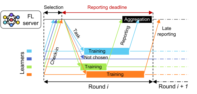
The training of the global model is conducted over a series of rounds. As shown in Fig. 1, at the beginning of each training round, the server waits (during a selection window) for a sufficient number of available learners to check-in. Then, the server samples a subset of the checked-in learners – called participants – to train in the current round. The participants fetch the latest version of the model along with any necessary configurations (e.g., hyper-parameter settings).

Each participant trains the model on its local data for a specified number of epochs and produces a model update (i.e., the delta from the global model) which it sends to the server. The server waits until a target number of participants send their updates to aggregate them and update the global model. This concludes the current round and the former steps are repeated in each round until a certain objective is met (e.g., target model quality or training budget).

To ensure progress, the server generally waits for model updates until a reporting deadline. Updates from stragglers that may arrive beyond the deadline are discarded. A round is considered successful if at least a target number of participants’ updates are received by the deadline, else the round is aborted and a new one is attempted.

The FL setting is also distinct from conventional ML training because the distributed learners may exhibit the following types of heterogeneity: 1) data heterogeneity:learners generally possess variable data points in number, type, and distribution; 2) device heterogeneity:learner devices have different speeds owing to different hardware and network capabilities; 3) behavioral heterogeneity:the availability of learners varies across rounds and there may be learners that abandon the current round if they become unavailable.

Heterogeneity creates several challenges for FL system designers because both the quality of the trained model and the training speed are majorly affected by which participants are selected at each round. Below we briefly review existing designs that serve as context to motivate our distinct approach (§3). We discuss additional related work in §8.

2.2. Existing FL Systems

Accounting for the unreliability of learners, SAFA (Wu et al., 2021) enables semi-asynchronous updates from straggler participants.

SAFA flips the participant selection process of FedAvg: it runs training on all learners and ends a round when a pre-set percentage of them return their updates. SAFA allows participants to report after the round deadline, in which case the updates are cached and applied in a later round. However, SAFA only tolerates updates from learners that are within a bounded staleness threshold. Therefore, the round duration in SAFA is reduced by only waiting for a fraction of the participants, while the cache ensures that the computational effort of straggling participants is not entirely wasted and is able to boost statistical efficiency. FLeet (Damaskinos et al., 2020) enables stale updates but adopts a dampening factor to give smaller weight as staleness increases. This is beneficial for not discarding updates that exceed the staleness threshold. However, their AdaSGD protocol is not directly compatible with the traditional FL settings such as FedAvg and FLeet synchronizes model gradients after every local mini-batch.

Oort (Lai et al., 2021) uses a participant selection algorithm that favors learners with higher utility. The utility of a learner in Oort is comprised of statistical and system utility. The statistical utility is measured using training loss as a proxy while system utility is measured as a function of completion time. Oort preferentially selects fast learners to reduce the round duration. At the same time, it uses a pacer algorithm that can trade longer round duration to include unexplored (or slow) learners when required for statistical efficiency.

3. The Case for Resource-Efficient FL

We motivate REFL by highlighting the trade-offs between system efficiency and resource diversity as conflicting optimization goals in FL. Navigating the extremes of these two objectives, as exhibited by the SOTA FL systems, we show how they fall short on common FL benchmarks.

3.1. System Efficiency vs. Resource Diversity

Current FL designs either aim at reducing the time-to-accuracy (i.e., system efficiency) (Lai et al., 2021) or increasing coverage of the pool of learners to enhance the data distributions and fairly spread the training workload (i.e., resource diversity) (Xie et al., 2020; Li et al., 2020a; Wu et al., 2021), but do not consider the cost of wasted work by learners. The first goal results in a discriminatory approach towards certain categories of learners, either preferentially selecting computationally fast learners or learners with model updates of high quality (i.e., those with high statistical utility) (Li et al., 2020a; Lai et al., 2021). The second goal entails spreading out the computations ideally over all available learners but at the cost of potentially longer round duration (Xie et al., 2020; Wu et al., 2021) and significant wasted work.

These two conflicting goals present a challenging trade-off for designers of FL systems to navigate. On one side of the extreme, Oort aggressively optimizes system efficiency and ignores the diversity of learners’ data in order to improve time-to-accuracy. The implication of this extreme is less robustness to high levels of data heterogeneity due to poor selection fairness, potentially producing a global model that does not cover the majority of learners’ data. On the other hand, SAFA foregoes pre-training selection, selecting all available learners to maximize resource diversity, at the cost of significantly increased resource wastage.

To strike a balance between the two extremes, the FL system should achieve a sufficient level of resource diversity without sacrificing significantly in terms of system efficiency. Our goal is to synthesize the opportunities presented by existing systems and devise a new holistic approach that can fulfill the resource diversity and system efficiency goals simultaneously while considering cumulative resource usage as a primary metric. We first show that the existing systems fail to achieve both of these goals and result in significant wastage of resources. We also highlight the opportunities they present which we embrace in our design of REFL.

3.2. Stale Updates & Resource Wastage

Figure 2. Resource usage comparison of SAFA versus an ideal resource-optimized version denoted as SAFA+O, and FedAvg with 10 or 100 participants. We train the model up to a target accuracy. The run time of each approach is shown as a colored annotation near the final data point.

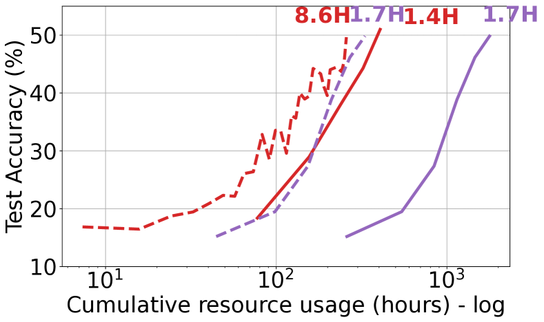
Taking inspiration from asynchronous methods (Ho et al., 2013; Xie et al., 2020), SAFA allows straggling participants to contribute to the global model via stale updates. We first evaluate SAFA’s resource usage (i.e., the time cumulatively spent by learners in training), and resource wastage (i.e., the time cumulatively spent by learners producing updates that are not incorporated into the model). We compare the performance of SAFA as described in (Wu et al., 2021) against a version (called SAFA+O) that assumes a perfect oracle that knows which stale updates are eventually aggregated (i.e., will not exceed the staleness threshold). We set the staleness threshold to 5 rounds and the target participant percentage to $10\%$. We use an audio dataset of spoken words provided by Google, hereafter referred to as the Google Speech benchmark (Warden, 2018), and use FedScale’s data-to-learner mappings (Lai et al., 2022) (c.f. Table 1 and Section 5 for details). We set the total number of learners to 1,000, and the round deadline to 100s. We use a real-world user behavior trace to induce learner’s availability dynamics (Yang et al., 2021).

Fig. 2 shows the resource usage (x-axis) and resulting test accuracy (y-axis); the lines are annotated with the time to achieve the final accuracy (this style is repeated in other figures in this paper). Since the round time is bounded by a deadline, both SAFA and SAFA+O have equal run times. Notably, SAFA is inefficient in terms of resource usage, consuming nearly 5$\times$ the resources of SAFA+O to achieve the same final accuracy. By selecting all available learners, then eventually discarding a large number of the computed updates, SAFA wastes around 80% of learners’ computation time. The plot also includes runs of FedAvg with Random selection of 10 and 100 participants. Despite having low resource wastage, FedAvg with 10 participants incurs significantly higher run time (5$\times$) to reach the same accuracy of SAFA; the resource usage could be traded for lower run time with 100 participants, to achieve the same accuracy at similar resource usage to SAFA+O. We note that uniform random data mapping yields similar results.

Opportunity.  In principle, allowing stale updates enables a reduction in round duration and achieves better time-to-accuracy while preserving stragglers’ contribution. The main challenge is, however, to balance the number of participants to avoid significant resource wastage. This is difficult because the system must estimate the on-device training time and reason about the probability of learners dropping out or exceeding the staleness threshold. This suggests that beyond stale updates, we must also tackle resource diversity directly.

(a) FedScale data mapping

(b) Label-limited (non-IID)

Figure 3. Impact of data heterogeneity on test accuracy in two data mappings. The right y-axes and dotted lines indicate the percentage of unique participants during training.

3.3. Participant Selection & Resource Diversity

Many existing FL systems select participants using a uniform random sampler (Caldas et al., 2019; Yang et al., 2018a; Bonawitz et al., 2019a). As noted in Oort (Lai et al., 2021), this simple strategy is prone to select learners with disparate computing capabilities and prolong round duration due to stragglers. On the other hand, Oort’s approach of selecting fast learners has unfavorable consequences, by biasing the model to a subset of the learners that can reduce data diversity.

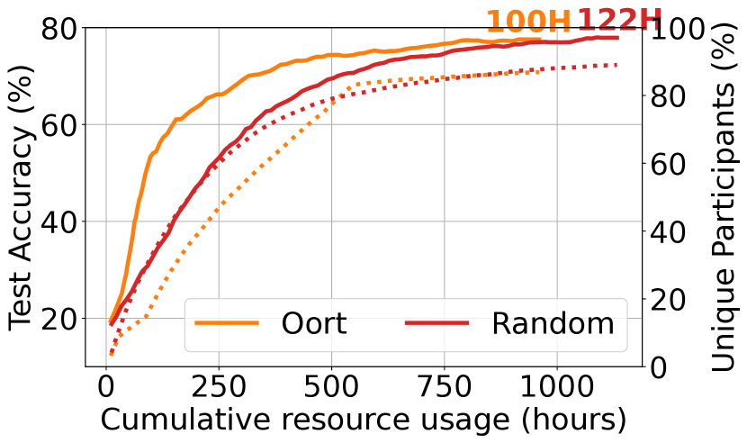
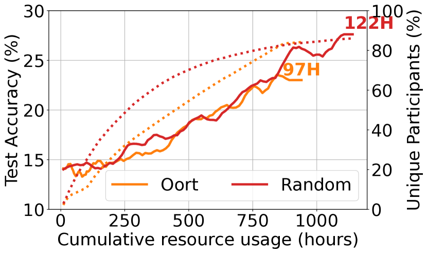
To see this in practice, we compare the Oort participant selector with a random sampler (Random). We use the Google Speech benchmark for 1,000 training rounds and compare two cases with different data mappings. In the first case, data points are mapped to the learners using FedScale’s client-to-data mappings (Lai et al., 2022). In the second case, data points are also uniformly distributed among the participants but each participant is constrained to have $\approx$10% of all labels (non-IID). To emphasize the effect of the sampling strategy, we set all learners to be always available; we investigate the effects of availability dynamics later.

Fig. 3 shows the resulting test accuracy against resource usage. In the FedScale’s data mapping scenario, Oort is clearly superior to random selection as Oort significantly reduces the round duration by exploiting fast learners. Conversely, in the non-IID case (label-limited mapping), random selection achieves higher accuracy with a tolerable increase in run time due to a higher resource (and data) diversity.

Participant availability impacts the global data distribution represented in the global model (Huang et al., 2022). Our analysis of a large-scale device behavior trace from (Yang et al., 2021) involving more than 136K users of an FL application over a week reveals that 70% of the learners are available for at most 10 minutes while 50% are available for at most 5 minutes. This means in practice FL rounds should typically last a few minutes to obtain updates from the majority of participants. The analysis also suggests that low availability learners may require special consideration to increase the number of unique participants without adversely impacting overall training time.

(a) FedScale data mapping

(b) Label-limited (non-IID)

Figure 4. Impact of availability on test accuracy in two data mappings.

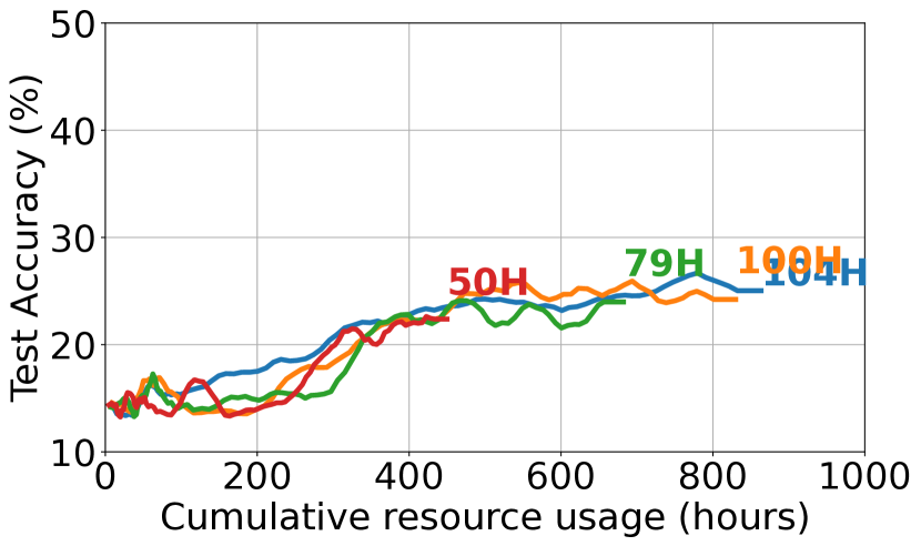
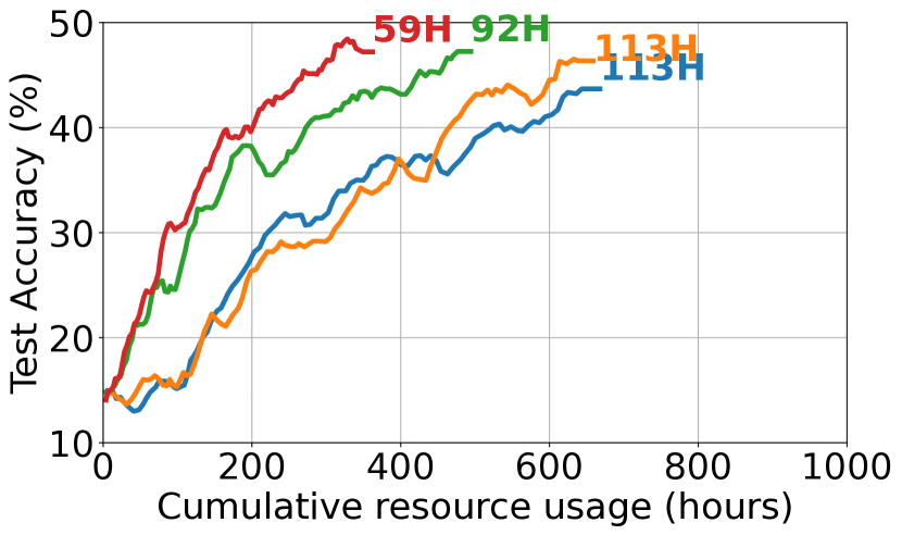
We now repeat similar experiments on the FedScale and non-IID cases of the Google Speech benchmark and contrast the execution of Oort and Random participant selection methods in two conditions: 1) all learners are available (AllAvail); 2) learners’ availability is dynamic based on the trace of device behavior (DynAvail). Fig. 4 shows that learner availability has no tangible impact in the FedScale case since learners hold data points with comparable distributions. However, in the non-IID case, learners’ availability has a significant effect on model accuracy (we observe a 10-point drop).

Opportunity.  To achieve better model generalization performance, the model should be trained jointly on data samples from a large fraction of the learner population. While Oort’s insights into informed participant selection result in faster round duration, there needs to be more consideration with regard to the dynamic availability of learners to ensure wider learner coverage. This suggests that beyond learners’ diversity and compute capabilities, we need to effectively prioritize learners whose availability is limited.

Figure 5. Example trace of 4 training rounds illustrating the main differences between Oort (b) and REFL (c). The dynamic availability of 9 color-coded learners is shown in (a). By optimizing for time-to-accuracy, Oort skews participant selection towards faster learners during the early phases of training, thereby missing limited-availability learners ($\blacksquare$ and $\blacksquare$). Oort’s round time is determined by stragglers. By allowing stale updates, REFL lowers the dependency on stragglers. By prioritizing learners based on estimated availability, REFL samples a more diverse set of learners.

4. REFL Design

REFL’s objective is to enhance the resource efficiency of the FL training process by maximizing resource diversity without sacrificing system efficiency. REFL achieves this by reducing resource wastage from delayed participants and prioritizing those with reduced availability. It leverages a theoretically-backed method to incorporate stale updates based on their quality which helps improve the training performance. It proposes a scaling rule for aggregation weights to mitigate stale updates’ impact.

The two core components of REFL are:

1. Intelligent Participant Selection (IPS): to prioritize participants that improve resource diversity.

2. Staleness-Aware Aggregation (SAA): to improve resource efficiency without impacting time-to-accuracy.

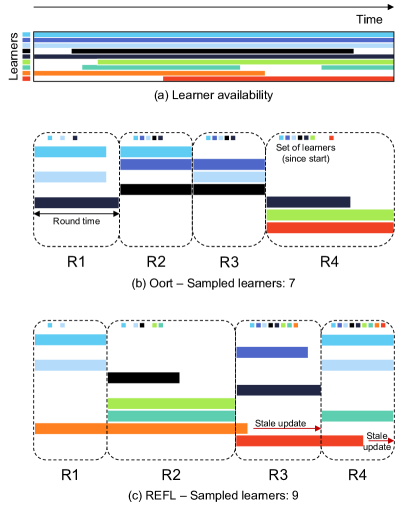
Overview by example.  To illustrate the main differences, Fig. 5 contrasts REFL with Oort. First, REFL enables learners’ tracking of the availability patterns which help with predicting the future availability. Therefore REFL is able to prioritize the least available participants (i.e., $\blacksquare$ and $\blacksquare$ in Fig. 5) to maximize training coverage of different learners’ data distributions. REFL also allows straggling participants to submit late results beyond the set round duration (i.e., $\blacksquare$ and $\blacksquare$ in Fig. 5). Unlike Oort, which discards these updates due to their inferior device capabilities, this approach reduces the wasted work of stragglers who might own valuable data for the model to be trained on.

4.1. Intelligent Participant Selection (IPS)

IPS increases resource diversity to allow the global model to capture a wide distribution of learners’ data. Moreover, it provides an optional component to further reduce resource wastage by intelligently adapting the number of participants in every round.

Input : $N_{t}$-Target number of participants

Output : $S$-List of selected participants

Initialize $S_{t}=\emptyset$, $P_{t}=\emptyset$, $a=(\mu_{t},2\mu_{t})$;

on event Learner_Check_In:

       Send slot $a$ to learner $l$;

       Receive learner $l$’s availability probability $p_{l}$;

       $P_{t}=P_{t}\cup p_{l}$;

      

on event End_Selection_Window:

       Sort in ascending order $P_{t}$;

       Randomly shuffle $P_{t}$ for probabilities with ties;

       Return $S_{t}$ as the top $N_{t}$ learners in $P_{t}$;

      

Algorithm 1 Priority Selection Algorithm

Least available prioritization:  Algorithm 1 describes how the IPS component intelligently selects participants from the large pool of available learners. Each learner periodically trains a model that predicts its future availability.Upon check-in of the learner $l$, the server sends the running average estimate of round duration $\mu_{t}$. The learner uses the prediction model to determine the probability of its availability in the time slot $[\mu_{t},2\mu_{t}]$ and reports this to the server. At the end of the selection window, the server sorts, in ascending order, the learners’ probabilities $P$ and randomly shuffles tied learners. Then, the server selects the top $N_{t}$ learners to participate in this round (i.e., the least available learners). Similar to Google’s FL system (Bonawitz et al., 2019a), the participants hold from checking-in with the server for few rounds (e.g., 5 rounds) after submitting the updates.

Availability prediction model:  A prediction model should be simple with low overhead and trained locally on the learners’ devices to preserve privacy. In this work, we do not propose new availability models and use off-the-shelf time-series models to predict the future availability of the learners. Linear models such as Auto-Regressive Integrated Moving Average (ARIMA) or Smoothed ARIMA can be trained on a minimal set of features collected from on-device events of change in the state such as idle, charging, connection to WIFI, screen locked, etc (Hyndman et al., 2002; Hyndman and Athanasopoulos, 2021). We use the Prophet forecasting tool (Taylor and Letham, 2017), which is based on the aforementioned linear models. We train a prediction model on the Stunner dataset, which is a large-scale dataset comprising device events from a large number of mobile users (e.g., the charging state of the devices) (Szabó et al., 2019). Given a time window in the future, the model produces a probability for the charging state (eq. availability) of the device within the queried time window. In §5, we show that the trained model can provide availability predictions with high accuracy.

Adaptive Participant Target (APT):  IPS can optimize resource usage by adapting the pre-set target number of participants $N_{0}$ selected by the operator. First, the server updates its moving average estimate of round duration $\mu_{t}=(1-\alpha)D_{t-1}+\alpha\mu_{t-1}$, where $D_{t-1}$ is the duration of the previous round $t-1$. Then, before commencing round $t$, the server probes each current straggler $s\in L_{s}$ (from round $t-1$) for an estimate of its expected remaining time to upload the update $RT_{s}$. Next, the server computes how many stragglers ($B_{t}$) can complete within the duration of the current round (i.e., $RT_{s}\leq\mu_{t}$). And so, the target number of participants is adjusted for round $t$ to $N_{t}=max(1,N_{0}-B_{t})$. This ensures that, in each round, a roughly constant number of updates $N_{0}$ is aggregated (i.e., the total fresh and stale updates). In large-scale scenarios, this could potentially further improve resource consumption. Note, irrespective of clients’ availability, APT is an add-on scheme to not over-commit the participants, further reducing resource consumption.

4.2. Staleness-Aware Aggregation (SAA)

This component enables the participants to submit their updates past the round deadline and processes these stale updates along-with the fresh updates. Stale updates can be noisy since the model can drift significantly by the time a stale update arrives. In order to mitigate this impact, we multiply the stale updates based on a boosting factor (§4.2.3).

We also provide a convergence analysis to substantiate the benefits of staleness. We analyze this effect independently of other REFL components because all the REFL components complement each other. Since FedAvg (McMahan et al., 2017; Bonawitz et al., 2019a) is one of the most prominent FL algorithms, we analyze (§4.2.2) FedAvg with staleness (termed Stale Synchronous FedAvg, c.f. Algorithm 2). Under standard assumptions, our convergence analysis shows that the error due to staleness is small in each round, and hence the gradient does not differ significantly (see Lemma 4). Due to this small error per round, we show in Theorem 1 that Stale Synchronous FedAvg converges at the same asymptotic rate as FedAvg.

4.2.1. Convergence Analysis

We theoretically demonstrate that FedAvg with stale updates can converge and obtain the convergence rate. Consider the following federated optimization problem consisting of a total of $m$ devices:

(1) $$\textstyle\min_{x\in\mathbb{R}^{d}}f(x)\mathrel{\vbox{\hbox{\scriptsize.}\hbox{\scriptsize.}}}=\frac{1}{m}\sum_{j\in[m]}f_{j}(x),$$

where $f_{i}(x)=\mathbb{E}_{z_{i}\sim{\mathcal{D}}}{l(x;z_{i})}$ such that $l(x;z_{i})$ denotes the loss function evaluated on input $z_{i}$ sampled from ${\mathcal{D}}$.

Algorithm 2 gives the pseudo-code of Stale Synchronous FedAvg to solve (1). Here, $g_{t,k}^{i}$ denotes the stochastic gradient computed at the $i^{th}$ participant at round $t$, and at local iteration $k$, such that $\textstyle g_{t,k}^{i}=\nabla f(y_{t,k}^{i})+\xi_{t,k}^{i}$ with $\mathbb{E}[\xi_{t,k}^{i}|x_{t,k}^{i}]=\mathbf{0}$.

Input : $K$-synchronization interval, $\tau$-delay in rounds, $N_{t}$-number of participants

Initialize $x_{0}=x_{1}=\ldots=x_{\tau-1}\in\mathbb{R}^{d}$

for round $t=0,\ldots,T-1$ do

       The server samples $S_{t}$ learners with $|S_{t}|=N_{t}$

       for participant $i\in[n]$ in parallel do

             $y_{t,0}^{i}=x_{t}$

             for iteration $k=0,\ldots,K-1$ do

                   Compute a stochastic gradient $g_{t,k}^{i}$

                   $y_{t,k+1}^{i}=y_{t,k}^{i}-\gamma g_{t,k}^{i}$

                    // Local participant update

                  

            Let $\Delta_{t}^{i}=y_{t,K}^{i}-y_{t,0}^{i}=-\gamma\sum_{k=0}^{K-1}g_{t,k}^{i}$

             Send $\Delta_{t}^{i}$ to the server

            

      At Server:

       if $t<\tau$ then

             Broadcast $x_{t+1}$ to participants

              // Aggregation starts $t=\tau$

            

      else

             Receive $\Delta_{t-\tau}^{i},i\in S$

              // Update arrives with delay $\tau$

             Let $\Delta_{t-\tau}=\frac{1}{|S|}\sum_{i\in S}\Delta_{t-\tau}^{i}$

             Server update: $x_{t+1}=x_{t}+\gamma\Delta_{t-\tau}$

             Broadcast $x_{t+1}$ to participants

            

      

Algorithm 2 Stale Synchronous FedAvg

The staleness of model updates is modeled as a round delay. For ease of exposition, we consider a fixed $\tau$ round delay in Algorithm 2. However, our analysis holds for variable delays bounded by $\tau$.

Assumptions:  we consider the following general assumptions on the loss function.

Assumption 1.

(Smoothness) The function, $f_{i}:\mathbb{R}^{d}\to\mathbb{R}$ at each participant, $i\in[n]$ is $L$-smooth, i.e., for every $x,y\in\mathbb{R}^{d}$ we have, $f_{i}(y)\leq f_{i}(x)+\left<\nabla f_{i}(x),y-x\right>+\frac{L}{2}\lVert y-x\rVert^{2}$.

Assumption 2.

(Global minimum) There exists $x_{\star}$ such that, $f(x_{\star})=f^{\star}\leq f(x)$, for all $x\in\mathbb{R}^{d}.$

Assumption 3.

(($M,\sigma^{2}$) bounded noise) (Sebastian U. Stich and Sai Praneeth Karimireddy, 2020) For every stochastic noise $\xi_{t,k}^{i}$, there exist $M\geq 0,\sigma^{2}>0$, such that $\mathbb{E}[\lVert\xi_{t,k}^{i}\rVert^{2}\mid x_{t}]\leq M\lVert\nabla f(x_{t,k}^{i})\rVert^{2}+\sigma^{2}$, for all $x_{t}\in\mathbb{R}^{d}$.

4.2.2. Convergence Result

The next theorem provides the non-convex convergence rate.

Theorem 1.

Let Assumptions 1, 2, and 3 hold. Then, for Algorithm 2, we have

$$\frac{1}{nTK}\sum_{t=0}^{T-1}\sum_{i=1}^{n}\sum_{k=0}^{K-1}\mathbb{E}\lVert\nabla f(y_{t,k}^{i})\rVert^{2}=$$

$$\textstyle{\mathcal{O}}\left(\frac{\sigma\sqrt{L(f(x_{0}-f^{\star}))}}{\sqrt{nTK}}+\frac{\max\{L\sqrt{\tau K(n\tau K+M)},L(K+M/n)\}}{TK}\right).$$

Overview of analysis.  Our analysis builds on top of the Error Feedback framework (Sebastian U. Stich and Sai Praneeth Karimireddy, 2020), which is in turn inspired by Perturbed Iterate Analysis (Mania et al., 2017). We first define the update of Stale Synchronous FedAvg:

(2) $$v_{t}=\begin{cases}0,&\text{if }t<\tau\\ \frac{1}{n}\sum_{i=1}^{n}\sum_{k=0}^{K-1}g_{t-\tau,k}^{i},&\text{otherwise.}\end{cases}$$

Using this definition of $v_{t}$, we have

(3) $$x_{t+1}=x_{t}-v_{t}\quad\forall t.$$

Let us also define the error $e_{t}$ due to asynchrony as

(4) $$e_{t}=\sum_{j=1}^{\tau}\mathbb{1}_{(t-j)\geq 0}\left(\frac{\gamma}{n}\sum_{i=1}^{n}\sum_{k=1}^{K}g_{t-j,k}^{i}\right).$$

where $\mathbb{1}_{Z}$ denotes the indicator function of the set $Z$.

The recurrence relation in the next lemma is instrumental for perturbed iterate analysis of Algorithm 2.

Lemma 0.

Define the sequence of iterates $\{\tilde{x}_{t}\}_{t\geq 0}$ as $\tilde{x}_{t}=x_{t}-\bar{e}_{t}$, with $\tilde{x}_{0}=x_{0}$. Then $\{\tilde{x}_{t}\}_{t\geq 0}$ satisfy the recurrence: $\tilde{x}_{t+1}=\tilde{x}_{t}-\frac{\gamma}{n}\sum_{i=1}^{n}\sum_{k=0}^{K-1}g_{t,k}^{i}$.

Lemmas 3 and 4 are useful for bounding intermediate terms.

Lemma 0.

We have

$$\mathbb{E}_{t}\lVert\frac{1}{n}\sum_{i=1}^{n}\sum_{k=0}^{K-1}g_{t,k}^{i}\rVert^{2}\leq\frac{1}{n}\sum_{i=1}^{n}\sum_{k=0}^{K-1}(K+\frac{M}{n})\lVert\nabla f(y_{t,k}^{i})\rVert^{2}+\frac{K\sigma^{2}}{n},$$

where $\mathbb{E}_{t}[\cdot]$ denotes expectation conditioned on the iterate $x_{t}$, that is, $\mathbb{E}[\cdot|x_{t}]$.

Lemma 0.

With a constant step-size $\gamma\leq\frac{1}{2L\sqrt{\tau K(n\tau K+M)}}$, we have

$$\sum_{t=0}^{T-1}\frac{1}{n}\sum_{i=1}^{n}\sum_{k=0}^{K-1}\mathbb{E}\lVert\tilde{x}_{t}-y_{t,k}^{i}\rVert^{2}$$

$$\textstyle\leq\frac{1}{4L^{2}}\sum_{t=0}^{T-1}\frac{1}{n}\sum_{i=1}^{n}\sum_{k=0}^{K-1}\mathbb{E}\lVert\nabla f(y_{t,k}^{i})\rVert^{2}+\frac{\gamma^{2}}{n}T\tau K^{2}\sigma^{2}.$$

Lemma 0.

Let Assumptions 1, 2 and 3 hold. If $\{x_{t}\}_{t\geq 0}$ denote the iterates of Algorithm 2 for a constant step-size,
$\gamma\leq\min\{\frac{1}{2L\sqrt{\tau K(n\tau K+M)}},\frac{n}{2L(nK+M)}\}$, then

$$\frac{1}{nTK}\sum_{t=0}^{T-1}\sum_{i=1}^{n}\sum_{k=0}^{K-1}\mathbb{E}\lVert\nabla f(y_{t,k}^{i})\rVert^{2}\leq$$

$$\textstyle\frac{8}{\gamma TK}\left(f(x_{0})-f^{\star}\right)+\frac{4\gamma L\sigma^{2}}{n}+\frac{4\gamma^{2}L^{2}\tau K\sigma^{2}}{n}.$$

The above leads us to the stated theorem for an appropriate choice of parameters.

Significance of results.  We achieve a ${\mathcal{O}}(\frac{1}{\sqrt{nTK}})$ asymptotic rate, which improves with $K$, the number of local steps per round. In comparison, the Asynchronous algorithm of (Xie et al., 2020) does not improve with the number of local steps. Moreover, asynchrony (captured by $\tau$) only affects the faster decaying ${\mathcal{O}}(\frac{1}{T})$ term. Thus, Stale Synchronous FedAvg has the same asymptotic convergence rate as synchronous FedAvg (Sebastian U. Stich and Sai Praneeth Karimireddy, 2020), and hence achieves asynchrony for free. Furthermore, this asymptotic rate is better for Stale Synchronous FedAvg in practice, since the rate improves with $n$, the total number of learners contributing to an update, and staleness relaxation should result in more learners contributing to an update.

4.2.3. Mitigating the Impact of Increased Staleness

We note that our convergence guarantee in §4.2.1 depends on the maximum round delay $\tau$, and large round delays could negatively impact convergence, which must be mitigated. To mitigate the impact, prior work on distributed asynchronous training proposes to scale the weight of stale updates before aggregation (Zhang et al., 2016; Jiang et al., 2017; Damaskinos et al., 2020). We denote the set of fresh and stale updates in a round as ${\mathcal{F}}$, and ${\mathcal{S}}$ respectively. Let $n_{{\mathcal{F}}}$ be the number of fresh updates, and $\hat{u}_{{\mathcal{F}}}$ be the average of the fresh updates. Moreover, let $n_{\mathcal{S}}$ be the number of stale updates, and for a straggler $s\in{\mathcal{S}}$, $u_{s}$ be the stale update, and $\tau_{s}$ be the number of rounds the straggler is delayed by. The following are the scaling rules in the literature:

1. Equal: same weight as fresh updates (i.e., $w_{s}=1$);

2. DynSGD: linear inverse of the number of staleness rounds $w_{s}=\frac{1}{\tau_{s}+1}$ (Jiang et al., 2017);

3. AdaSGD: exponential damping of the number of staleness rounds $w_{s}=e^{-(\tau_{s}+1)}$ (Damaskinos et al., 2020).

AdaSGD also proposed a boosting multiplier to increase the weights for stale updates to account for learners with data distributions that more significantly deviate from the global data distribution. AdaSGD showed that boosting the weight of important stale updates is critical since stragglers may possess more valuable (dissimilar) data compared to fast learners. However, this approach may violate privacy because computing the boosting factor requires learners to share information about their data.

Therefore, we propose a privacy-preserving boosting factor and combine it with the staleness-based damping rule of DynSGD (Jiang et al., 2017). The proposed boosting factor favors a stale update based on how much it deviates from the fresh updates’ average and hence it does not require any information about learner’s data. Let, $\Lambda_{s}=\frac{\lVert\hat{u}_{\mathcal{F}}-\frac{u_{s}+n_{\mathcal{F}}\hat{u}_{f}}{n_{\mathcal{F}}+1}\rVert^{2}}{\lVert\hat{u}_{{\mathcal{F}}}\rVert^{2}}$ be the deviation of the stale update $u_{s}$ from the average of the fresh updates $\hat{u}_{{\mathcal{F}}}$. Let $\Lambda_{max}=\max_{s\in{\mathcal{S}}}{\Lambda_{s}}$. The boosting factor term scales a stale update $s$ proportional to $1-e^{-\frac{\Lambda_{s}}{\Lambda_{max}}}$. Finally, our rule to compute the scaling factor is:

(5) $$\textstyle w_{s}=(1-\beta)\frac{1}{\tau_{s}+1}+\beta(1-e^{-\frac{\Lambda_{s}}{\Lambda_{max}}})$$

where $\beta$ is a tunable weight for the averaging.

For every fresh update $f\in{\mathcal{F}}$, we choose a scale value of one, i.e., $w_{f}=1$. The final coefficients for weighted averaging are the normalized weights. That is, for an update $i\in{\mathcal{F}}\cup{\mathcal{S}}$, the final coefficient as:

$$\hat{w}_{i}=\frac{w_{i}}{\sum_{i\in{\mathcal{F}}\cup{\mathcal{S}}}w_{i}}$$

Hence, in aggregation, $w_{i}<w_{f}$ meaning that weights applied to stale updates are strictly less than weights for new updates. This in principle reduces the impact from malicious learners who delay the updates to gain any advantage because of the boosting factor. Further analysis in adversarial settings is left to future work.

Table 1. Summary of benchmarks and characteristics of the mappings used in this work.

Task

Model

Dataset

Model Size # of Parameters

Learning Rate

Local Epochs

Batch Size

# of Labels

FedScale Mapping

Label-limited Mapping

# of samples

Total Learners

# of samples

Total Learners

# of Labels

Image Classification

ResNet18 (He et al., 2016)

CIFAR10 (Krizhevsky, 2009)

11.4M

0.01

1

10

10

N/A

N/A

50K

3K

4

ShuffleNet (Zhang et al., 2018)

OpenImage (Kuznetsova et al., 2020)

2.23M

0.01

5

30

600

1.3M

14K

1.3M

3K

60

Speech Recognition

ResNet34 (He et al., 2016)

Google Speech (Warden, 2018)

21.5M

0.005

1

20

35

200K

3K

200K

3K

4

Natural Language Processing

Albert (Lan et al., 2020)

Reddit (Pushshift, 2020)

11M

0.0001

5

40

N/A

42M

16M

8.4M

3K

N/A

Stackoverflow (McMahan et al., 2017)

11M

0.0008

5

40

N/A

43M

300K

8.6M

3K

N/A

5. Evaluation

Our evaluation addresses the following questions:

• Is prioritizing learners based on availability beneficial?

• Does aggregation of stale updates reduce resource usage and improve model quality?

• Should stale updates be weighted differently to fresh updates?

• Is REFL scalable and future-proof?

We summarize the main observations as follows:

• REFL achieves better model quality with up to 2$\times$ less resources compared to existing systems.

• REFL results in quality gains in different scenarios involving both IID and non-IID scenarios.

• REFL’s weight scaling boosts the statistical efficiency.

• REFL scales well and is more robust in future scenarios.

5.1. Experimental Setup

Our experiments simulate FL benchmarks consisting of learners using real-world device configurations and availability traces. Our experiments capture different scenarios, models, datasets and data distributions as detailed next. We use a cluster of NVIDIA GPUs to interleave the training of the emulated learners. The participants train in parallel on time-multiplexed GPUs using PyTorch v1.8.0.

Implementation:  We implement REFL within FedScale (Lai et al., 2022), a framework for emulation and evaluation of FL systems. The SAA and IPS components are implemented as Python modules and integrated into FedScale’s server aggregation logic and participant selection procedures, respectively. We defer to §7 a discussion on deployment considerations and integration with popular FL frameworks.

Emulation environment:  Our results are gathered via emulation in FedScale. This framework comprises three key components:

1) The Aggregator selects participants, assigns the task, and handles the aggregation of updates. It employs a Client Manager to track learners’ availability and selects the target number of participants in each round. It also employs an Event Monitor which processes system events and invokes the appropriate event handler.

2) The Executor runs the learners’ logic, loads the corresponding federated dataset, and trains the model using the PyTorch backend. The latency is determined for computation by # of samples $\times$ latency per sample, and for communication by size in bytes $/$ bandwidth. This allows for having a simulated run time using realistic traces.

3) The Resource Manager manages the available computational resources (e.g., GPUs). It employs a queue for the learners waiting for training on the computing resource and assigns a learner to the first available computing resource.

Benchmarks:  We experiment with the benchmarks listed in Table 1, that span several common FL tasks of different scales to cover varied practical scenarios. The datasets consist of hundreds or up to millions of data samples, we refer the reader to (Lai et al., 2022, 2021) for the description of the datasets. As in (Lai et al., 2021), by default, FedAvg (McMahan et al., 2017) is used as the aggregation algorithm for CIFAR10, and YoGi (Ramaswamy et al., 2020) for other benchmarks.

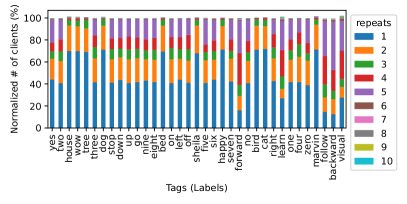
Data partitioning:  To account for realistic heterogeneous data mappings, we partition the labeled training dataset among the learners using different methods, from easy to hard. As commonly done in the literature, the baseline case is a random uniform mapping (IID). Second, we adopt the FedScale data-to-learner mappings (Lai et al., 2022), which encompass thousands to millions of learners whose data distribution reflects real data sources. However, upon analyzing the frequency of label appearances across learners in the FedScale data mapping for the Google speech benchmark (c.f. Fig. 6), we observe that most labels appear at least once on more than $40\%$ of the learners, making this close to a uniform distribution, and thus simplifying training. Similar observations are made for CV benchmarks.

Figure 6. Number of label repetitions across learners.

To consider other realistic heterogeneous data mappings, we introduce label-limited mappings where learners are assigned data samples drawn from a random subset of labels as listed in Table 1, with data samples per learner following particular distributions as follows. L1) Balanced distribution: using an equal number of samples for each data label on each learner; L2) Uniform distribution: using uniform random assignment of data points to labels on each learner; L3) Zipf distribution: Zipfian distribution with $\alpha=1.95$ to have higher level of label skew (popularity).

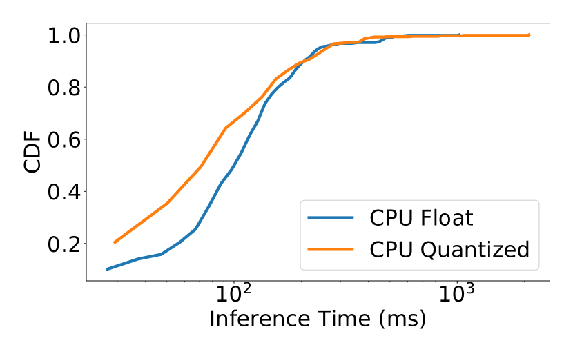
System performance of learners:   Learners’ hardware performance is assigned at random from profiles of real device measurements from the AI (Benchmark, 2021) and MobiPerf (M-Lab, 2021) benchmarks for inference time and network speeds of mobile devices, respectively. AI Benchmark catalogs inference times for popular DNN models (e.g., MobileNet) on a wide range of Android devices (e.g., Samsung Galaxy S20 and Huawei P40). The profiles include devices with at least 2GB RAM using WiFi, which matches the common case in FL settings (Yang et al., 2018a; Bonawitz et al., 2019a; Lai et al., 2021).

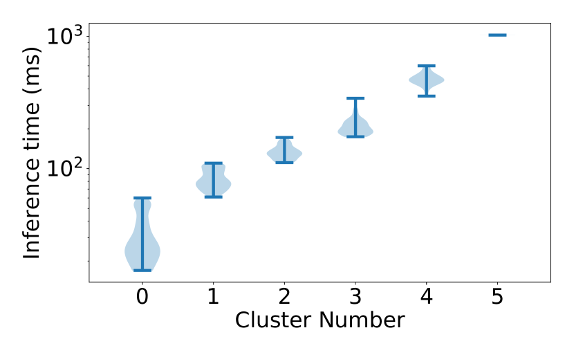
We show how the distribution of floating-point and quantized inference times from the AI benchmark and device profiles can be clustered into 6 different device configurations demonstrating significant device heterogeneity with a long tail distribution, as shown in Fig. 7(a). Fig. 7(b) shows that learners could be grouped into 6 clusters of different device configurations according to their computational capabilities, demonstrating that learners can have highly variable completion time during training.

(a) CDF of inference time

(b) Clustering of devices

(c) Available learners over time

(d) CDF of availability period

Figure 7. Computational [(a),(b)] and availability [(c),(d)] characteristics of learners’ profiles used in experiments.

(a) FedScale’s data mapping

(b) Label-limited (balanced)

(c) Label-limited (uniform)

(d) Label-limited (Zipfian)

(e) Percent. of unique learners

(f) # of aggregated updates

Figure 8. Training performance comparison under OC+DynAvail across different data mappings.

(a) Balanced

(b) Uniform

(c) Zipfian

Figure 9. Training convergence comparison under OC+DynAvail across the different Label-limited (non-iid) data mappings.

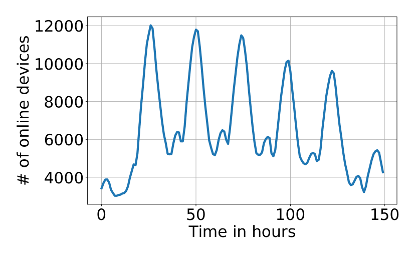
Availability dynamics of learners:   We use a trace of 136K mobile users from different countries over a period of 1-week (Yang et al., 2021). The trace contains $\approx$180 million entries for events such as connecting to WiFi, charging the battery, and (un)locking the screen. Availability is defined as when a device is plugged to a charger and connected to the network, similar to (tensorflow.org, 2020; Lai et al., 2021).

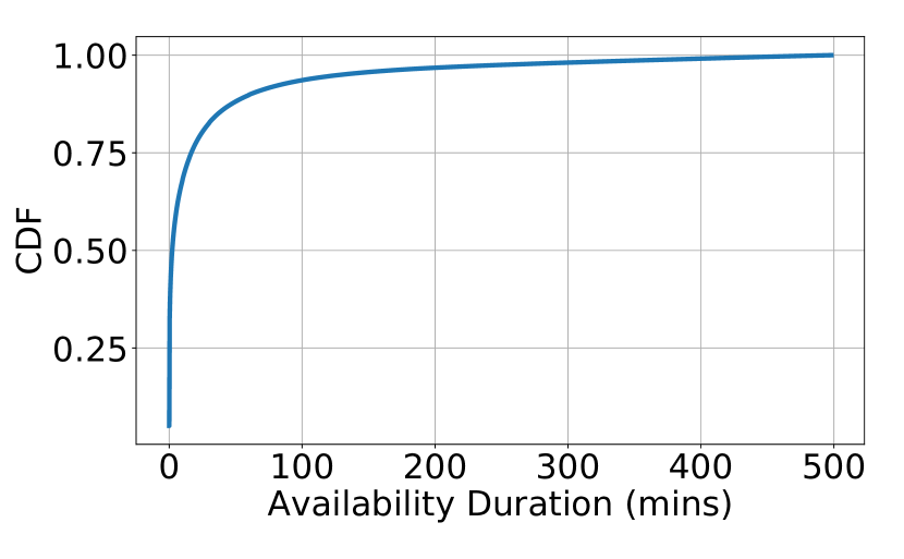
We see that learners exhibit variations (and cyclic behavior) and most learners stay available for only a few minutes. We extract availability dynamics from the user behavior trace in (Yang et al., 2021). Fig. 7(c) shows that the number of available learners over time varies significantly and they exhibit a diurnal pattern over the days of the week where large numbers of learners are mostly available (i.e., charging) during the night. Fig. 7(d) shows a CDF of the length of learners’ availability slots which exhibits a very long tail. Most clients (up to 70%) are available for less than 10 minutes.

Hyper-parameter settings:  The FL and learning hyper-parameters were the default values set by the FedScale framework and no further tuning was done. The common FL hyper-parameters were the same for all methods in the comparison. We used the recommended parameter settings for the evaluated methods (i.e., Oort (Lai et al., 2021) and SAFA (Wu et al., 2021)).

REFL parameters:  Unless otherwise stated, no maximum threshold is applied to staleness when incorporating updates. We set $\alpha=0.25$ for the moving average of round duration which is chosen to give more weight to the most recent round duration values. We set $\beta=0.35$ for the weight of stale updates in Eq. 5 to favour dampening over scaling the stale updates. We tested, within our experimental capacity, different values and found the aforementioned values worked well. We leave a detailed sensitivity analysis and ablation study of hyper-parameters to future work.

Availability prediction model:  In the experiments, we assume the model has 90% accuracy for future availability (i.e., 1 out of 10 selections is a false positive), which matches the model accuracy obtained from training a simple linear model on real-world trace as detailed in Section 5.2.

(a) Uniform mapping (iid)

(b) Label-limited (uniform)

Figure 10. Comparison against SAFA.

Experimental scenarios:  We consider two experimental settings used in the literature:

1. OC: the FL server over-commits the target number of participants $N_{t}$ by 30% and waits for the updates from $N_{t}$ participants (as in (Lai et al., 2021, 2022));

2. DL: the FL server chooses a target number of participants $N_{t}$ and aggregates any number of updates received before the end of a pre-set reporting deadline (as in (Yang et al., 2021; Bonawitz et al., 2019a)).

Unless otherwise mentioned, the target number of participants is 10; each experiment is repeated 3 times with different sampling seeds and the average of the three runs is shown. The experiments use $\approx$13K hours of GPU time.

5.2. Experimental Results

We evaluate the amount of learner resources (and run time) spent to achieve a certain test accuracy (lower resources and lower run time are better). Since our results are based on emulation, we quantify resource usage using the time accumulated at every learner as a proxy. In particular, the cumulative resources for each round are computed as the cumulative sum of computation and communication time for all participants in the round.

Here, we focus on Google Speech and present the results of other benchmarks and experimental settings in §5.2.8. Table 2 show the baseline accuracy of the benchmarks in a semi-centralized training setting (i.e., data-parallel) where the dataset is uniformly divided among 10 learners that participate in every training round.

(a) AllAvail

(b) DynAvail

Figure 11. Training performance of REFL with Adaptive Participant Target using 50 participants in OC and different availability.

(a) FedScale data mapping

(b) Label-limited (uniform)

Figure 12. Performance comparison of REFL vs Oort vs Random in the OC+AllAvail experimental setting.

(a) Uniform random
(IID)

(b) FedScale mapping

(c) Label-limited (uniform)

(d) Label-limited
(Zipfian)

(e) Label-limited (balanced)

Figure 13. Performance of various scaling rules for stale update weighting in the aggregation step.

Table 2. Baseline performance with centralized training.

Benchmark	Quality Metric	Aggregation Algorithm	Data to Learner Mapping
			Uni. Rand.	Label-limited
				Uni. Rand.	Zipf Dist.	Balanced
CIFAR10	Top-5 Test Acc	FedAvg	90.4	86.1	76.4	86.4
Open Image	Top-5 Test Acc	YoGi	70.7	30.6	32.3	35.5
Google Speech	Top-5 Test Acc.	YoGi	76.5	34.7	33.4	37.1
Reddit	Test Perp.	YoGi	43.6	N/A	N/A	N/A
Stackoverflow	Test Perp.	YoGi	40.2	N/A	N/A	N/A

5.2.1. Performance of selection algorithms

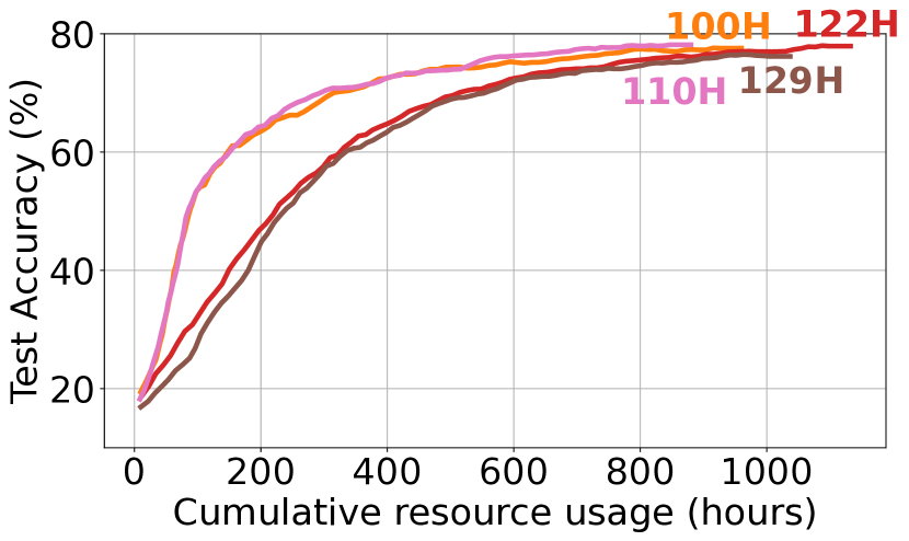
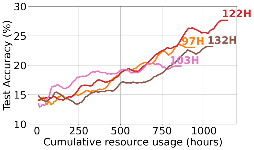
We use the experimental setting OC+DynAvail. We compare REFL with Oort, Random, and Priority selection. Priority is the IPS component of REFL (i.e., SAA component is disabled).

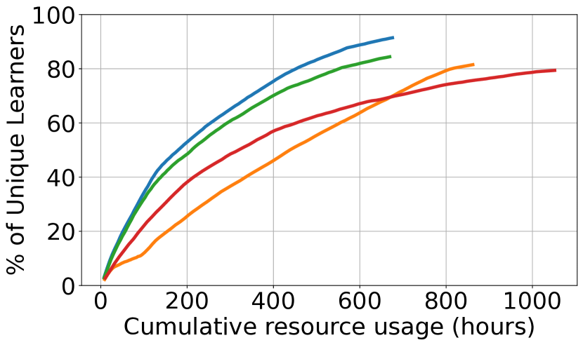
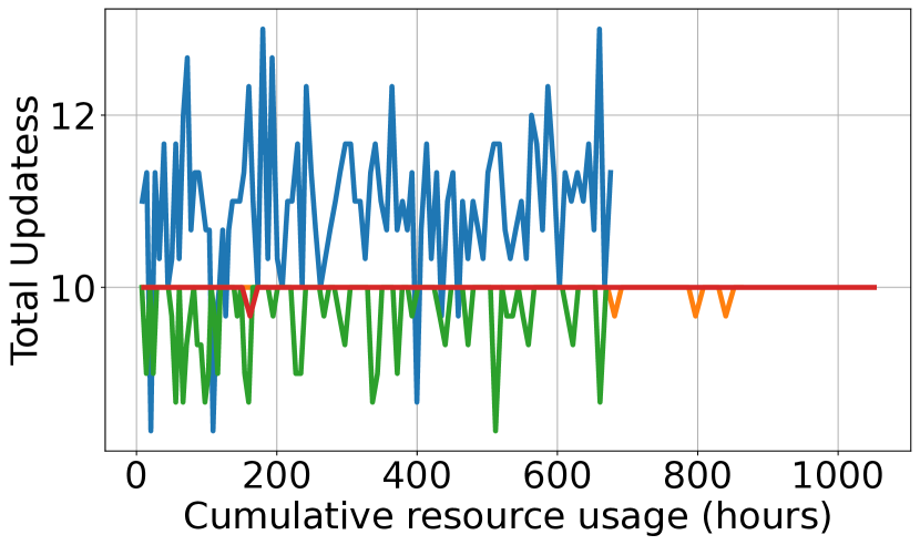
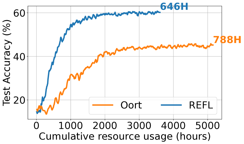
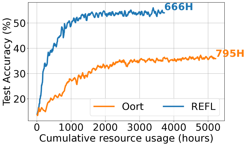
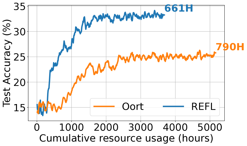
Fig. 8 shows that, over the FedScale and different non-IID (label-limited) data mappings, with minimal resource usage, REFL achieves better accuracy over other methods (i.e., Oort, Random, and Priority). REFL achieves superior performance thanks to the availability-based prioritization (Fig. 8(e)) and aggregation of stale updates (Fig. 8(f)). When the FL training process is run for more rounds in the label-limited non-IID case, Fig. 9 shows that REFL converges to significantly higher accuracy than Oort, in less time and with lower resource usage.

5.2.2. Performance of aggregation algorithms

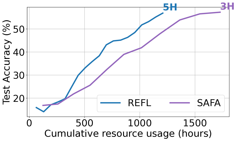
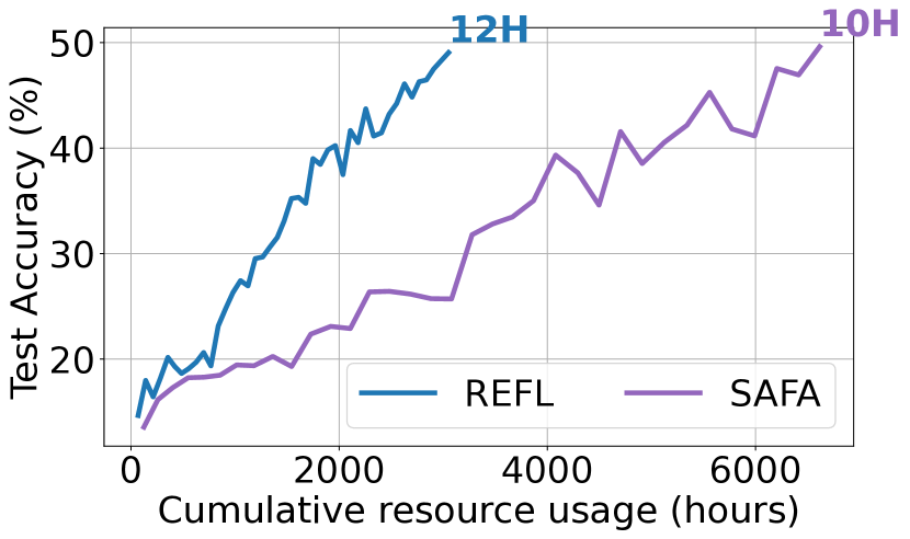
Comparing SAFA and REFL, we use the DL+DynAvail setting with a total learner population of 1,000 and a round deadline of 100s. We use FedAvg as the underlying aggregation algorithm. REFL pre-selects 100 participants and the target ratio is set to $10\%$ and $80\%$ for SAFA and REFL, respectively. For both schemes, we set the staleness threshold to 5 rounds.

The results in Fig. 10 show that run times of SAFA and REFL are comparable, but SAFA consumes significantly more resources. In the case of the FedScale mapping (Fig. 10(a)), the results show that REFL achieves higher accuracy with $\approx\!20\%$ fewer resources than SAFA. In the non-IID mapping (Fig. 10(b)), REFL significantly improves the accuracy by 10 points using $\approx\!60\%$ fewer resources compared to SAFA.

(a) Reddit

(b) StackOverFlow

(c) OpenImage

(d) CIFAR-10

Figure 14. Performance for NLP and CNN benchmarks in OC+DynAvail. We use the Label-limited mapping for Stackoverflow and Reddit, FedScale data mapping for OpenImage and Uniform IID mapping for CIFAR10.

5.2.3. Availability-based prioritization

The results in Fig. 8 show that Priority selection achieves better model accuracy thanks to prioritizing the least available learners. The results suggest that, especially in non-IID settings, selecting participants with low availability results in a better rate of unique learners with valuable (likely new) data samples, and hence the resource usage to achieve a certain accuracy is also reduced.

5.2.4. Adaptive target

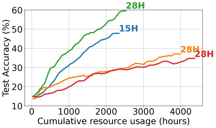
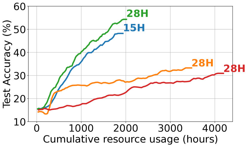
We run experiments in the OC setting with both DynAvail and AllAvail scenarios using the label-limited (uniform) mapping and 50 participants per round.

Fig. 11 shows that, in both scenarios, REFL and REFL +APT have higher model quality with lower resource usage compared to Oort and Random. Moreover, the resource consumption of REFL can be further reduced with APT by trading off extra run time (i.e., 15H vs. 28H). Compared to AllAvail, the improvements are maintained in DynAvail when REFL prioritizes the least available clients and comparable accuracy is achieved. However, depending on the benchmark, APT may yield no benefits when the target number of participants is small (e.g., $N_{0}\leq 10$).

5.2.5. Stale aggregation

We experiment with REFL, Oort, and Random in the OC+AllAvail setting.

Fig. 12 shows the achieved test accuracy vs training rounds. We observe that, over different data mappings, REFL achieves good model quality with lower resource usage thanks to the SAA component. Notably, the benefits are more profound for non-IID distributions. In non-IID settings, the stale updates of delayed participants are more important compared to IID settings. This demonstrates that stale updates can boost the statistical efficiency of training. Also, REFL achieves run time similar to Random because learners have their availability probability set to 1 (always available), and so REFL reverts to random selection.

5.2.6. Stale weight scaling

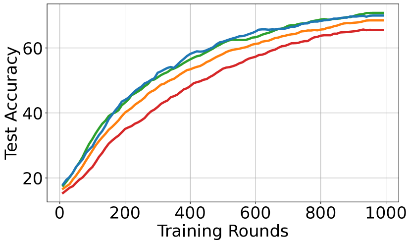
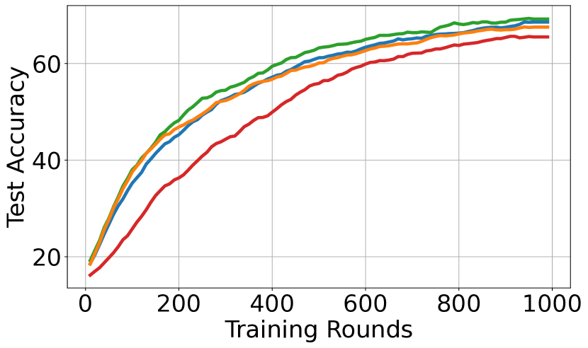
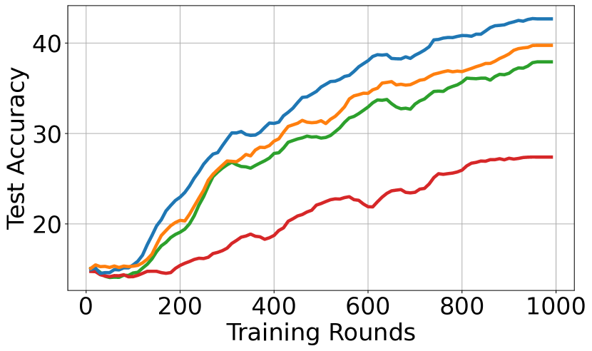
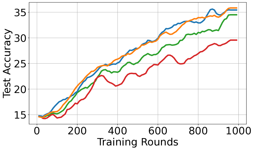
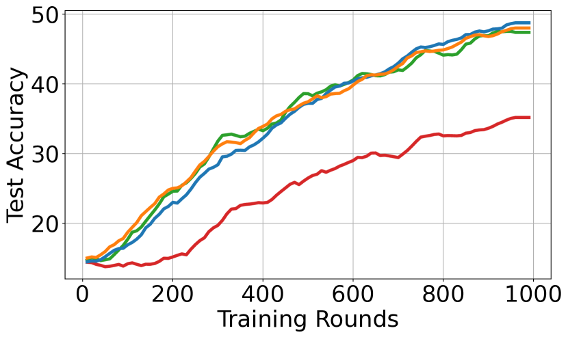
We use OC+DynAvail and set the deadline to 100 seconds. We evaluate the weight scaling rules of §4.2.3 and present test accuracy results over the training rounds in Fig. 13.

We observe that the REFL’s scaling rule consistently outperforms the other scaling rules in all data distribution scenarios. In the IID cases (Figs. 13(a) and 13(b)), the differences among the scaling rules are small. However, in the non-IID cases (Figs. 13(c), 13(d) and 13(e)), the performance is inconsistent except for REFL’s rule. These results show the benefits of REFL’s rule for mitigating the potential negative impact of stale updates. The same observations are made for OC+AllAvail with FedAvg.

5.2.7. Availability prediction model

We evaluate the forecasting model. The model is trained on the Stunner trace (Szabó et al., 2019), which contains device events from large number of worldwide mobile users. We used devices with at least 1,000 samples (i.e., 137 devices) in the trace collected during September 2018. We extracted the plugged-in and charging state to train a model for each device using the first half of each devices’ samples. We compared the devices’ model predictions on the remaining samples, which are thus used as the testing dataset.

The results show that the models predict future availability states with high accuracy. The values of the coefficient of determination, mean square error and mean absolute error, averaged across devices, are 0.93, 0.01, and 0.028, respectively.

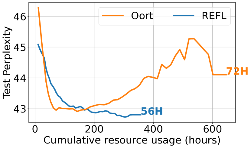
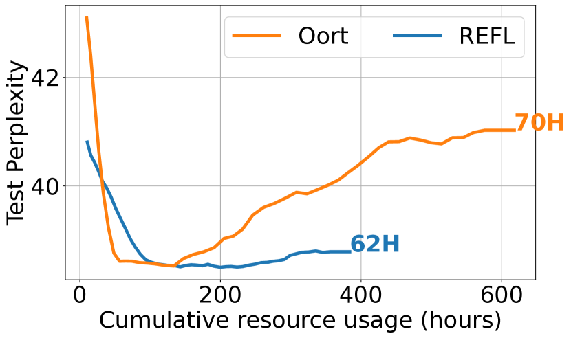
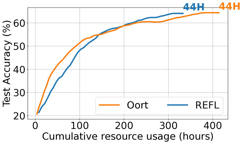
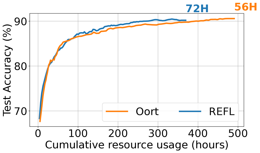
5.2.8. Results of other benchmarks

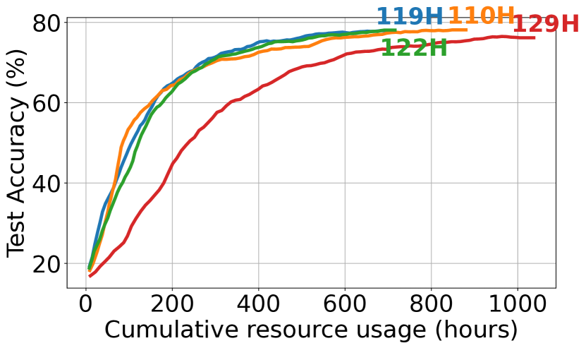
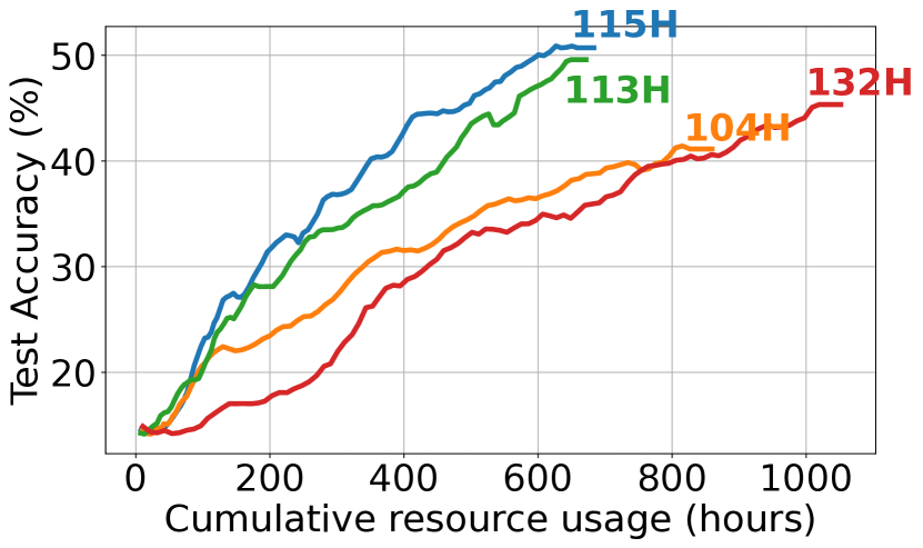
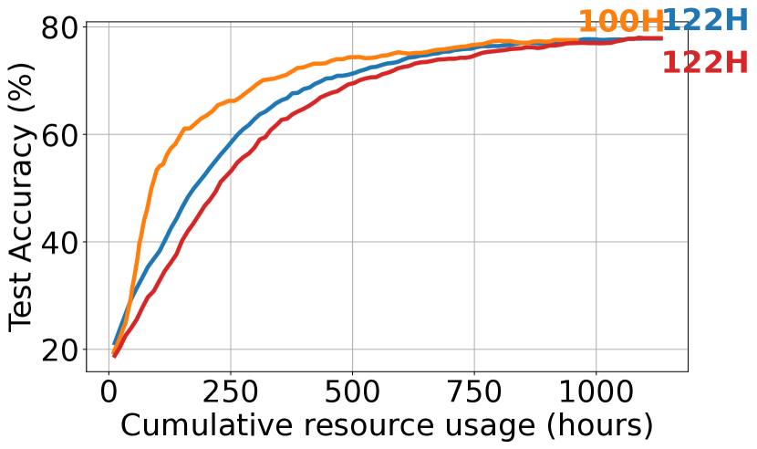
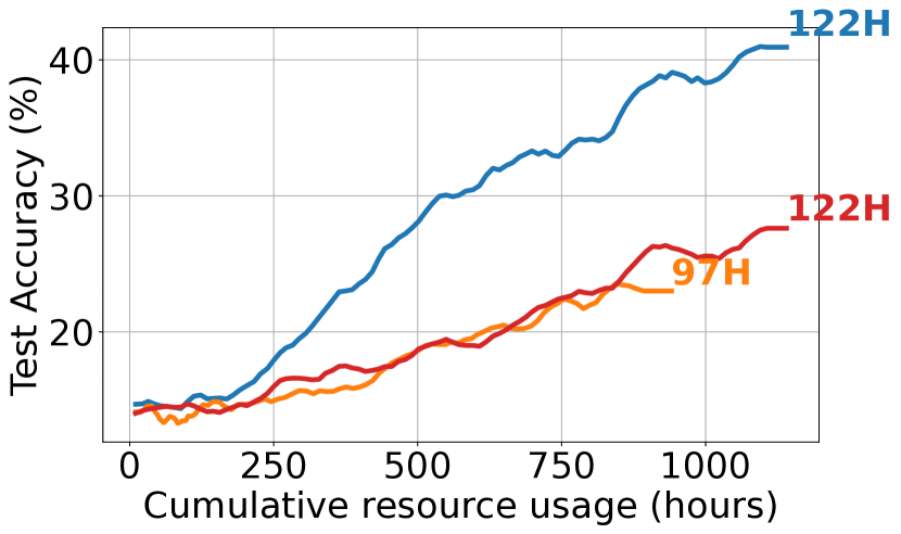
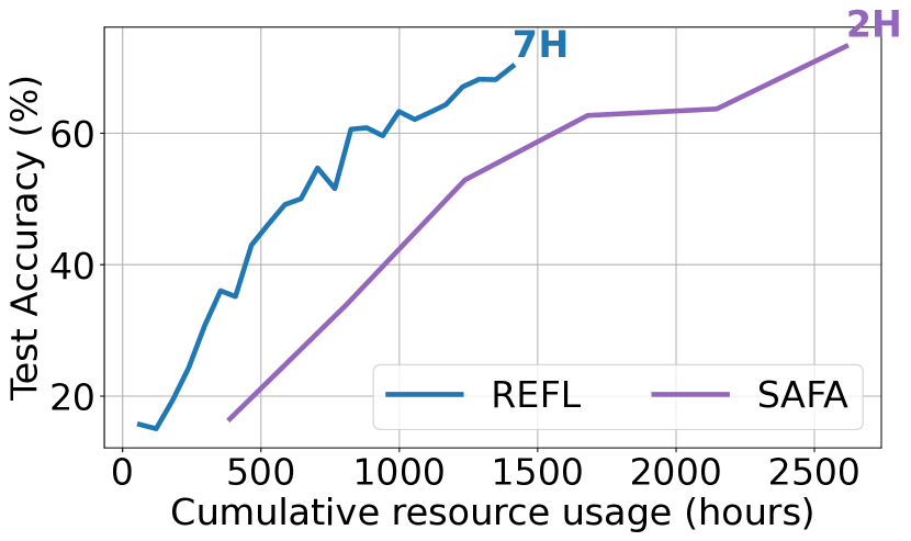
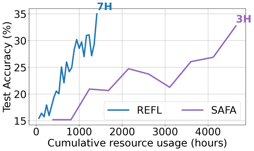
We run NLP (Reddit and StackOverFlow) and CV (CIFAR10 and OpenImage) benchmarks in the OC+DynAvail setting. We use YoGi as the aggregation algorithm for the Open Image, Reddit and StackOverFlow benchmarks and FedAvg for the CIFAR10 benchmark. Adaptive Participant Target (APT) is enabled for REFL. We also limit NLP dataset sizes to 20% (i.e., $\approx$ 8 million samples) as indicated in Table 1.

The results in Fig. 14 directly compare REFL and Oort. The results for Reddit (Fig. 14(a)) and StackOverFlow (Fig. 14(b)) demonstrate that REFL achieves considerable reduction in both learners’ resource consumption and the final test perplexity compared to Oort. We note that during the initial rounds, the performance is comparable between REFL and Oort. Then, Oort’s low diversity results in divergence which may be attributed to the lack of new samples (or participants with new data which help improve the model convergence). Similarly, the results for OpenImage (Fig. 14(c)) and CIFAR10 (Fig. 14(d)) show that REFL achieves the same model accuracy with lower resource consumption compared to Oort in scenarios when the data distribution among the learners is IID or FedScale’s data mapping (i.e., closer to IID).

6. Discussion

We discuss the implications of REFL in future scenarios.

Large-scale federated learning:  We project that future FL deployments will scale significantly to include learner devices such as sensors, IoT devices, autonomous vehicles, etc., that may not be connected to power sources and have limited computational capabilities. REFL enables efficient scaling over a larger number of resources, in contrast to FL systems that perform post-training selection (e.g., SAFA) or skew participant selection to fast devices (e.g., Oort). Invoking all devices for training would overwhelm the server and impose significant energy usage by learners, much of which would be wasted.

We show the impact of large populations on resource usage using the Google speech benchmark and 3$\times$ the number of learners (3,000). As shown in Fig. 15, we observe that SAFA wastes many resources in the IID (Fig. 15(a)) and even more in the non-IID (Fig. 15(b)) setting.

(a) Uniform mapping
(IID)

(b) Label-limited
(uniform)

Figure 15. Resource efficiency in large-scale FL settings.

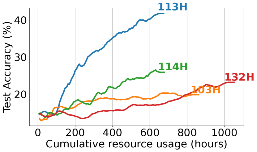
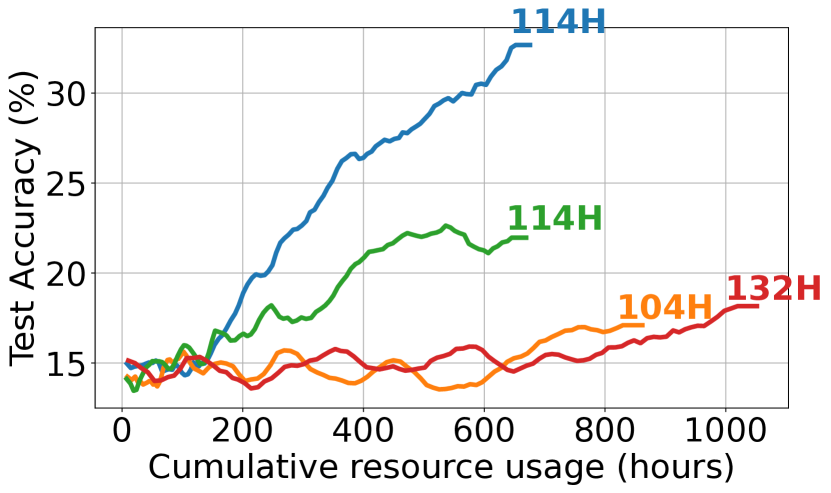
Future hardware advancements:  We project that computational capability of devices will continue to improve and so FL systems should benefit from this. Therefore, schemes such as Oort that favor faster learners are likely to see increased under-representation of low-capability learners, resulting in models that do not generalize well over a large population. In contrast, REFL copes with hardware advancements by benefiting from faster learners without overlooking low-capability learners.

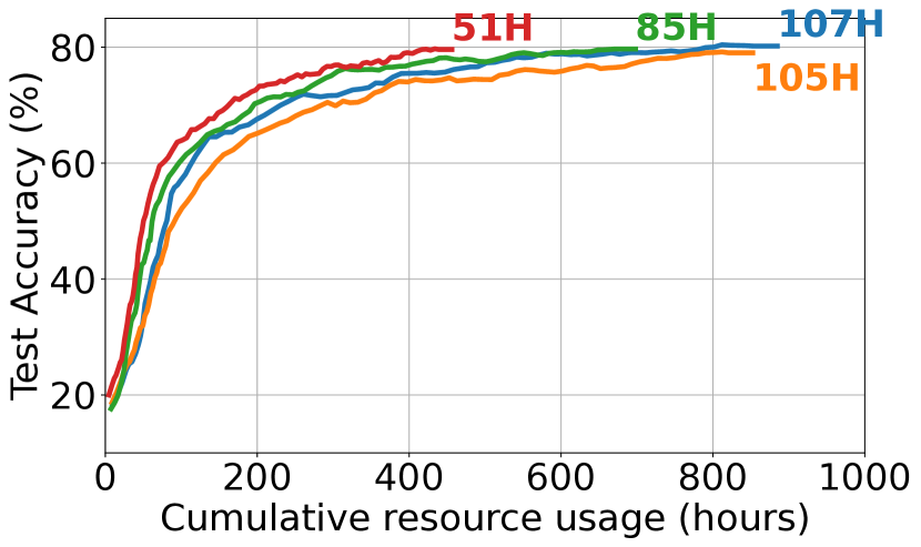
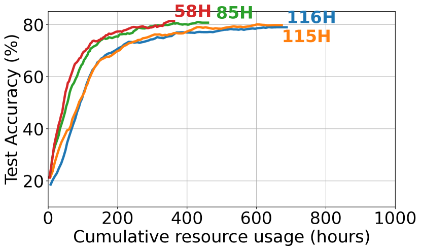
We run the Google Speech benchmark in 4 settings using: current device configurations (HS1); device configurations with completion times (i.e., computation and communication) doubled for the top $X$ percentile of devices (where $X$ is 25% (HS2), 75% (HS3), and 100% (HS4)). As shown in Figs. 16(a) and 16(b), we observe both Oort and REFL benefit from hardware enhancements in IID settings. However, as shown in Fig. 16(c), with realistic label-limited non-IID settings, REFL sees significant performance benefits due to the aggregation of stale updates and higher participant diversity. Oort does not benefit from improved speeds because the selection still favors the faster learners, which reduces training time but not model quality.

Implications of the availability prediction model:  When new learners join the FL process, they may not have traces with which to train their availability prediction model, resulting in low confidence in their predictions. Moreover, malicious or adversarial laerners may attempt to influence the system by consistently reporting low future availability. To deal with these scenarios, and as recommended by (Bonawitz et al., 2019a), we use in Section 4.1 a filtering mechanism that prevents a participant to be reselected in the following $X$ rounds (in our experiments 5 rounds).

(a) Oort - Uniform (IID)

(b) REFL- Uniform (IID)

(c) Oort - Label-limited uniform

(d) REFL- Label-limited uniform

Figure 16. Impact of future hardware advancements.

7. Integration with FL Frameworks

The design of REFL is lightweight and can operate as an online service or a plug-in module for existing FL frameworks. Therefore, REFL suits large-scale FL deployments dealing with likely thousands to millions of end-devices.

REFL selects participants as follows: 1) First, the server updates its estimate of round duration $\mu_{t}$ and send an estimate of the time period $a=(\mu_{t},2\mu_{t})$ of the next round to the learners; 2) learners maintain a local trace of their charging events and periodically train the forecasting model, which produces a probabilistic value for their charging state during future time periods. 3) upon receiving an availability query $a$, each the learner $l$ uses the prediction model to produce its availability probability $p_{l}(a)$ during time period $a$ and sends $p_{l}(a)$ to the server; 4) the server collects the probabilities $P_{t}$ and selects the participants using Algorithm Algorithm 1; and 5) the server sends each of the selected participants a random hash ID which encodes a time-stamp of the current round as well as the FL task (e.g., the model) and relevant parameter configuration.

REFL handles stale updates as follows: i) The server collects the updates which are received before the end of current training round $t$. If the time-stamp of a received update’s hash ID does not match the the current round, it is categorized as a stale update; ii) at the end of the round during aggregation, the server aggregates the fresh updates first to produce $\hat{u}_{\mathcal{F}}$. iii) for each stale update, $u_{s}$, the server computes the level of staleness $\tau_{t}$ using the timestamp of the stale update $\hat{u}_{\mathcal{F}}$; iv) for each stale update, the server computes the deviation of the stale update from the fresh updates $\Lambda_{t}$ and uses the proposed rule in Eq. 5 to assign the scaling weight $w_{s}$ to the stale update; and v) the server aggregates the scaled stale updates with the aggregated fresh updates to produce the new model using Algorithm 2.

To integrate REFL with PySyft, minimal exchanges between the server and learners are needed at the selection stage. The server sends an estimate time-slot of the next training round. The learners use the forecasting model and send their availability probability. Therefore, the learners do not need to exchange any sensitive information about their data. The FL developer programs the client-side to train the forecasting model and respond to the availability query from the server which poses minimal memory and communication overhead. REFL can also run as a distributed service using a communication library (e.g., XML-RPC (Docs, 2020)) to establish the communication channel between the REFL process and the server. The server can share metadata from the participants with the REFL service. The server can use the PySyft API model.send(participant_id) to invoke the participants selected by REFL, and model.get(participant_id) to collect the model and metadata updates from the participant.

8. Related Work

Federated learning:  FL is commonly viewed as a ML paradigm wherein a server distributes the training process on a set of decentralized participants that train a shared global model using local data that is never communicated with other entities (McMahan et al., 2017; Kairouz et al., 2019). FL has been used to enhance prediction quality for virtual keyboards among other applications (Bonawitz et al., 2019a; Yang et al., 2018a). A number of FL frameworks have facilitated research in this area (Caldas et al., 2019; Ryffel et al., 2018; PaddlePaddle.org, 2020; tensorflow.org, 2020; Yang et al., 2021; Lai et al., 2022). Flash (Yang et al., 2021) extended Leaf (Caldas et al., 2019) to incorporate heterogeneity-related parameters. FedScale (Lai et al., 2022) enables FL experimentation using a diverse set of challenging and realistic benchmark datasets; we use it as the emulation framework in this work.

Participant selection strategies:  In each round, the FL server samples among online learners and trains the global model on the selected participants (e.g., 10s of learners) among those currently online (e.g., 1,000s of learners). A number of recent works have proposed enhanced participant selection strategies. Biasing the selection process towards learners with fast hardware and network speeds has been proposed (Nishio and Yonetani, 2019). Other work has sought to enhance statistical efficiency by selecting participants with better model updates (Ruan et al., 2021; Chen et al., 2020a; Cho et al., 2022). Recently, Oort (Lai et al., 2021) proposed a strategy that combines both system and statistical efficiency. As we demonstrate in this work, these approaches either result in wasted computation or low coverage of the learners.

Heterogeneity in FL:  A significant challenge facing wider adoption of FL systems at scale is uncertainties in system behavior due to learner, system, and data heterogeneity. Learners’ computational capacity can restrict contributions and extend round duration (Li et al., 2020a; Yang et al., 2021; Li et al., 2022; Abdelmoniem et al., 2022). Architectural and algorithmic solutions to tackle heterogeneity have been proposed (Abdelmoniem and Canini, 2021; Wang et al., 2020; Li et al., 2020a, 2021; Lai et al., 2021). Heterogeneity in FL is particularly challenging because participants have varying data distributions and availability, as well as heterogeneous system configurations that cannot be controlled (Yang et al., 2018a; Bonawitz et al., 2019a; Kairouz et al., 2019; Abdelmoniem et al., 2022).

FL proposals:  Broader improvements in FL systems have included reducing communication costs (Konečný et al., 2016; Smith et al., 2017; Bonawitz et al., 2019a; Chen et al., 2020b; Reisizadeh et al., 2020), improving privacy guarantees (McMahan et al., 2018; Melis et al., 2019; Bonawitz et al., 2019a; Nasr et al., 2019; Bagdasaryan et al., 2020), compensating for partial work (Li et al., 2020a; Wang et al., 2020), minimizing energy consumption on edge devices (Li et al., 2019b), and personalizing global models trained by participants (Jiang et al., 2019a). Recent works have sought to address the challenge of data heterogeneity (Mohri et al., 2019; Li et al., 2020b, a).

Our work complements these efforts aiming to optimize the FL ecosystem. We aim to produce a resource-efficient FL framework making better use of learners’ resources to achieve target model quality without stretching training time. REFL’s design can easily benefit from the existing techniques for secure aggregation or differential privacy.

9. Conclusion

We studied two key issues preventing the wider adoption of FL systems: resource wastage and low data diversity. We proposed REFL that addresses these issues through two core components that encompass novel selection and aggregation algorithms. Compared to existing systems, REFL is shown, both theoretically and empirically, to improve model quality while reducing resource usage with low impact on training time. REFL is a vital step towards establishing a novel and practical ecosystem for resource-efficient federated learning.