On the Markov extremal problem in the -norm with the classical weight functions
Gradimir V. Milovanović
Serbian Academy of Sciences and Arts, 11000 Beograd, Serbia &
Faculty of Science and Mathematics, University of Niš, 18000 Niš, Serbia
gvm@mi.sanu.ac.rs
Abstract.
This paper is devoted to Markov’s extremal problems of the form , where is the set of all algebraic polynomials of degree at most and is a normed space, starting with original Markov’s result in uniform norm on from the end of the 19th century. The central part is devoted to extremal problems on the space for the classical weights on , and
. Beside a short account on basic properties of the (classical) orthogonal polynomials on the real line, the explicit formulas for expressing -th derivative of the classical orthonormal polynomials in terms of the same polynomials are presented, which are important in our study of this kind of extremal problems, using methods of linear algebra. Several results for all cases of the classical weights, including algorithms for numerical computation of the best constants , as well as their lower and upper bounds, asymptotic behaviour, etc.,
are also given. Finally, some results on Markov’s extremal problems on certain restricted classes of polynomials are also mentioned.
Inequalities for polynomials and their derivatives, as well as the corresponding extremal problems, are very important in many areas in mathematics, but also in other computational and applied sciences. In particular they play a fundamental rule in Approximation Theory, e.g., inequalities of Markov and Bernstein-type are fundamental for the proofs of many inverse theorems in the so-called
Polynomial Approximation Theory. These inequalities and extremal problems can be considered in different, usually normed spaces. Several monographs have been published in this area (cf. [46, 13, 50]), as well as many papers111This paper is dedicated to the mathematical contribution of Professor Ravi Agarwal..
In this paper by we denote the set of all algebraic polynomials of degree at most , and by
the set of all polynomials of exact degree , so that
, and
will be the
set of all monic polynomials of degree , i.e.,
The first result in this area was
connected with some investigations of the
well-known Russian chemist Dmitri Mendeleev (1834–1907).
In mathematical terms, Mendeleev’s problem [38] was as follows:
If is an arbitrary quadratic polynomial defined on an interval , with
how large can be on ? It can be reduced to a simpler problem by changing the horizontal scale and shifting the coordinate axis until we have , so that Mendeleev’s problem becomes the following:
If is an arbitrary quadratic polynomial and
on , how large can be on ?
Mendeleev found that on . This result is the best possible because for we have and . The corresponding problem for polynomials from was solved by a very famous Russian academician Andrei Andreyevich Markov (1856–1922) at the end of the 19th century. Markov’s younger half-brother Vladimir Andreevich Markov (1871–1897), although he died young, gained also an international reputation because he later solved the problem for -th derivative
, . Both were students of the famous Pafnuty Lvovich Chebyshev (1821–1894) at St. Petersburg State University. Another member of the Russian mathematical school, a student of the French Sorbonne and of Jewish origin, is Sergei Natanovich Bernstein (1880–1968), whose results have left a deep mark on the development of this field.
This inequality is best possible and the equality is attained at only , and only when , where is a complex number such that , and is well-known Chebyshev polynomial of the first kind, defined by
Introducing the uniform norm for polynomials on as
then Markov’s result can be expressed in the form
(1.2)
It is known as Markov’s extremal problem in the uniform norm.
The equality is attained at the Chebyshev points
, ,
if and only if , where ,
and is best possible.
Note that this version of Bernstein’s inequality is a pointwise inequality, while Markov’s inequality
, ,
is global. Combining these inequalities, we get
The natural question is how large can be for a given , when and
on ? Such a function is evidently an even function on . Explicit expressions for and can be found in [46, pp. 539]. The determination of for is very complicated and it can be given by a technique of Voronovskaja [58].
Taking norms different from the uniform norm we can consider
Markov’s extremal problem in other spaces, e.g. in , or even in spaces with quasi-norms , etc.
One can also consider the so-called mixed Markov type inequalities on ,
when , where
Evidently, for is a quasi-norm of . For some extremal problems of this type see [33, 12, 26, 27, 28, 54].
For and the inequality is know as the Nikol’skiĭ inequality (see [46, pp. 495–507]).
For , the previous problem
reduces to finding a polynomial that deviates least from zero in the -metric
with a fixed leading coefficient. For example, when , , and , the solutions (extremal polynomials) are known: the Chebyshev polynomial of the first kind , the Legendre polynomial , and the Chebyshev polynomial of the second kind , respectively.
However, the set can be restricted to some of subsets , and then we can consider the corresponding Markov extremal problem on such restricted sets again in different norms (cf. [46, Chapters 5 & 6]).
In this paper we consider Markov’s extremal problems of the form
(1.5)
on the inner product functional space , with the inner product defined by
(1.6)
where is a non-negative function on , ,
for which all moments , , exist and . Such a function is known as the weight function on .
The norm of an element is given by
(1.7)
For in (1.5) we use terms the best, exact or sharp constant.
In particular, we treat the basic extremal problem for the first derivative, i.e., the determination of the best constant .
The paper is organized as follows. A short account on
basic properties of the orthogonal polynomials on the real line, and in particular for ones known as the “classical orthogonal polynomials”, is given in Section 2. Explicit formulas for expressing -th derivative of the classical orthonormal polynomials in terms of the same polynomials are presented in Section 3. Such formulas are important in our study of extremal problems (1.5) on for the classical weight functions on , , and in Section 4.
Special cases of Markov’s extremal problems for all classical weight functions are given in Sections 5–7. Finally, in Section 8 some results on Markov’s extremal problems on certain restricted classes of polynomials are mentioned.
2. Basic Properties of the Orthogonal and the Classical Orthogonal Polynomials
The orthogonal polynomials are basic tools in the investigation of the extremal problems (1.5) on the space , and therefore in the this section we give some basic properties of the orthogonal polynomials on the real line, including, in particular, an important class of the so-called very classical orthogonal polynomials (cf. [16, 25, 37]).
The inner product (1.6) gives rise to a unique system of orthonormal polynomials , such that
, with
for each ,
and
(2.1)
Also, we need here the monic orthogonal polynomials,
in notation,
Because of the property of the inner product , orthogonal polynomials on the real line satisfy a three-term recurrence relation (cf. [37, p. 99]).
(a) For orthonormal polynomials we have
(2.2)
with and , where the coefficients and are given by
(b) For monic orthogonal polynomials we have
(2.3)
with and , where the coefficients and are given by
These coefficients in the three-term recurrence relations (2.2) and (2.3)
depend only on the weight function . The coefficients , , in (2.3) are positive, and may be arbitrary, but sometimes it is convenient to define it by . Then, it is easy to see that
An important result on zero distribution of orthogonal polynomials on the real line is the following (cf. [37, p. 99]):
All zeros of , , are real and distinct and are located in the interior of . Furthermore, the zeros of and interlace, i.e.,
Here, denote the zeros of in increasing order.
Using procedures of numerical linear algebra, notably the QR or QL algorithm, it is easy to compute the zeros of the orthogonal polynomials rapidly and efficiently as eigenvalues of the Jacobi matrix of order associated with the weight function ,
(2.4)
Unfortunately, the recursion coefficients and in (2.3) are known explicitly only for some narrow classes of orthogonal polynomials. One of the most important
classes for which these coefficients are known explicitly are surely the
so–called very classical orthogonal polynomials, which appear frequently in applied analysis and computational sciences. Orthogonal polynomials for which the recursion coefficients are not known we call strongly non–classical polynomials.
2.1. Classical weight functions and the corresponding orthogonal polynomials
In the sequel we consider only very classical orthogonal polynomials, omitting the term “very” and call them simply the classical orthogonal polynomials. They are distinguished by several particular properties
(cf. [37, pp. 121–146]).
Their weight function, the so-called classical weight function on , satisfies a first order differential equation of the form
where is a first degree polynomial, and is one of degrees not greater than two. For such classical weights we will write , and for the classical orthogonal polynomials use a general notation . We note
that for such weights , we have , as well as
Without loss of generality, the classical polynomials orthogonal with respect to the inner product (1.6), can be considered only on
three different intervals: , , and , because every interval can be transformed by a linear transformation to one of the previous intervals. These three cases are presented in Table 1.
Table 1. Classification of the classical orthogonal polynomials.
The corresponding orthogonal polynomials are known as the Jacobi polynomials , the generalized Laguerre polynomials ,
and finally as the Hermite polynomials . Because of the existence of the moments, the parameters , and should be greater than . The classical orthogonal polynomial is a particular
solution of the following differential equation
, where
(2.5)
The corresponding values are for the Jacobi polynomials, for the generalized Laguerre polynomials, and for the Hermite polynomials.
The corresponding orthonormal classical polynomials will be denoted by small letters ; in particular, by , , and , and the monic polynomials as , i.e., by , , and .
There are several characterizations of the classical orthogonal polynomials (cf. [5]). One of them was given by Agarwal and Milovanović [1, 2]:
Theorem 2.1.
Let and . Then for all the inequality
(2.6)
holds, with equality if only if , where is the classical orthogonal polynomial and is an arbitrary constant.
An important property of the classical orthogonal polynomials is the following
result (cf. [37, pp. 124–126]):
Theorem 2.2.
The derivatives of the classical orthogonal polynomials , , with respect to the weight function , also form a sequence of the classical orthogonal polynomials
with respect to the weight function .
According to Theorem 2.2 and the uniqueness of orthogonal polynomials, the following formulas
(2.7)
(2.8)
(2.9)
hold.
3. Differentiation Formulas for the Classical Orthogonal Polynomials
In this section we give formulas for expressing -th derivative of the orthonormal classical polynomials
in terms of the same polynomials, i.e.,
For all classical polynomials we can get explicit formulas for the coefficients . Such expressions we use in our study of extremal problems (1.5), when . Namely, in our consideration of the Markov extremal problems for the classical weights we usually reduce them to eigenvalue problems on the finite-dimensional spaces generated by orthonormal polynomials. Therefore, we are interested in expressing the derivatives of the basis polynomials as a linear combination of exactly the same polynomials.
Now, we separately consider three classical cases (see
Table 1).
Hermite polynomials. In this case, using (2.9) we get
Thus,
(3.1)
Generalized Laguerre polynomials. In this case, we first easily can obtain that
Jacobi polynomials. In order to get an analogous formula of (3.3) for the Jacobi polynomials, we use the following expansion (cf. [6, Lemma 7.1.1, p. 357]), but written for the monic Jacobi polynomials,
(3.5)
where
(3.6)
(3.9)
Here is the generalized hypergeometric function, which is, in general, defined by (cf. [6, Chap. 2])
The function is implemented as HypergeometricPFQ in Wolfram’s Mathematica and suitable for both symbolic and numerical calculation.
Iterating (2.7), again for the monic Jacobi polynomials, we obtain
Finally, for the orthonormal Jacobi polynomials , we obtain
(3.10)
where
(3.11)
and is defined by
(3.12)
The leading coefficients of the orthonormal Jacobi polynomial , , are given by (cf. [37, p. 133])
(3.13)
In the simplest (Legendre) case, when (), the leading coefficient (3.13) reduces to
In four Chebyshev cases when , we have the following coefficients for the monic polynomials:
For the Chebyshev weight of the first kind :
;
For the Chebyshev weight of the second kind :
;
For the Chebyshev weight of the third kind
:
;
For the Chebyshev weight of the fourth kind :
.
The leading coefficients in the corresponding orthonormal polynomials for four Chebyshev cases are
4. Extremal Problems of Markov’s Type for Polynomials in –Norms for the Classical Weight Functions
In this section we consider Markov’s -extremal problem (1.5) on the space , i.e.,
(4.1)
with the inner product defined by (1.6), where is a classical weight function ().
In 1987 Milovanović [40] showed that the exact constant in (4.1) can be found as the maximal eigenvalue of a square matrix of Gram’s type or as the spectral norm of one triangular matrix.
Here we consider this extremal problem on , with the inner product defined by (1.6), where . As before, the corresponding classical orthonormal polynomials will be denoted by , . The main approach will be based on analysis of the differentiation operator , as a linear map and its matrix of type
, using the orthonormal basis in the finite-dimensional spaces , with and .
Let be an arbitrary real polynomial in , which can be uniquely represented in the orthonormal basis as
(4.2)
Then the differentiation operator , which maps elements (polynomials) from the -dimensional space to another -dimensional space , can be uniquely described by the images of all basis polynomials , , in the space , represented in the corresponding basis of orthonormal polynomials .
Since , we have
(4.3)
where
(4.4)
so that the matrix of the operator
is given by
(4.5)
where is a zero matrix of the type , and
is a real quadratic matrix of order . The columns in the matrix (4.5) are vectors whose coordinates are coefficients in the expansions of the images of , , in the basis .
The quadratic matrix in (4.5) can be interpreted as a matrix of the differentiation operator , denoted now as , which maps the space to . Both of these spaces are of the same dimensions, i.e., . Here, is a restriction of the operator from to . Thus, belongs
to the set of all linear operators from to , denoted by . If we denote by
the set of all quadratic matrices of order , then the mapping
is a bijection from onto (cf. [43, Chap. II]), and the extremal problem (4.1) can be considered by methods of linear algebra.
These symmetric matrices and are positive definite, so that the corresponding quadratic forms and are positive for all non-zero vectors and .
All eigenvalues of such matrices are positive numbers.
Now, for determining the best constant in (4.10) we use the well know result on the bounds for the quadratic form of a positive definite matrix ,
(4.11)
where and are the minimal and maximal eigenvalues of the matrix and is the standard Euklidean norm of the vector .
This is how we get to the main result.
Theorem 4.1.
The best constant for the Markov -extremal problem is given by
(4.12)
where is the maximal eigenvalue of the matrix , and is the upper triangular matrix , with elements given by
. An extremal polynomial is
(4.13)
where is the eigenvector of the matrix corresponding to the maximal eigenvalue
.
Alternatively,
(4.14)
where is the minimal eigenvalue of the matrix defined by .
Proof.
Applying (4.11) with and we obtain (4.12) and (4.14), respectively. Since left (right) inequality in (4.11) reduces to an equality if and only if is the eigenvector corresponding to the minimal (maximal) eigenvalue of the matrix , we obtain the extremal polynomial given by (4.13).
∎
In the following sections, we analyze the the corresponding extremal problems with the Hermite, the generalized Laguerre and the Jacobi weights, including results on algorithms for numerical computation of the best constants, as well as their lower and upper bounds, asymptotic behaviour, etc. obtained by several authors (cf. Milovanović [40], Dörfler [19], [20], [21], Draux and Kaliaguine [22], [23], Böttcher and Dörfler [14, 15], Aptekarev at al. [7], [9], [10], Nikolov and Shadrin [48, 49], etc.).
The elements of the matrix , defined in (4.7), are practically given by formulas derived in Section 3 for all .
5. Extremal Problem With the Hermite Weight
We consider now the Hermite weight on .
Theorem 5.1.
Let , with the Hermite weight . Then the best constant in is given by
(5.1)
with the extremal polynomial , where is a non-zero constant.
Proof.
According to (3.1), is a diagonal matrix of order , with diagonal elements
so that the matrix in (4.10) is also diagonal, with
eigenvalues , . Thus, using (4.12), we get the best constant
i.e.,
(5.1). The extremal polynomial is , where is a non-zero constant.
∎
The best constant in Markov’s extremal problem
on
for the first derivative was solved in 1944 by E. Schmidt [51] and later by Turán [56].
Remark 5.2.
Theorem 5.1 was also proved by Shampine [52, 53], Dörfler [18],
Milovanović [40], as well as by Guessab and Milovanović [31, 32] using different methods. For other results in this subject see [29, 30].
6. Extremal Problem With the Generalized Laguerre Weight
For considering Markov’s extremal problems (4.1) on the space , with the generalized Laguerre weight and the
inner product defined by (1.6), we use the expansion (3.3) for an arbitrary and (3.4) for .
Thus, the elements (4.4) of the matrix can be calculated as
using the explicit expression for given in (3.3).
The following commands in Wolfram’s Mathematica 12.3 provide this calculation, where the upper triangular matrix (4.7) is denoted by Ank[n,k,s],
as well as the matrices and/or
, that appear in Theorem 4.1. For example, for given , and , the matrix , its minimal eigenvalue and the best constant can be also obtained by the following commands in Mathematica,
In 1960 P. Turán [56] obtained the sharp constant for the first derivative in the explicit form for , i.e., when :
(6.1)
as well as the extremal polynomial
(6.2)
where is the Laguerre polynomial. Schmidt [51] also considered this problem and obtained that
where .
We note that in this simplest case , according to (3.4), the matrices and are given by
and
(6.3)
The last tridiagonal matrix can be interpreted as a Jacobi matrix given by (2.4) for certain sequence of monic orthogonal polynomials , , with respect to some weight function . These polynomials satisfy the three-term
recurrence relation
(6.4)
with , , where the coefficients are
, , , . Putting , i.e., , (6.4) is a linear difference equation of the second order, whose general solution is given by , where and are arbitrary constants.
Since and , we
obtain the particular solution
(6.5)
which enables us to find the eigenvalues of the matrix as the zeros of the polynomial
in the explicit form,
Since the minimal eigenvalue is , i.e.,
according to (4.14), the best constant in Turán’s case is given by (6.1).
It is easy to check that the , given by (6.2), is an extremal polynomial on .
Remark 6.1.
The polynomials in (6.5) can be expressed in terms of Chebyshev polynomials of the third kind , which are given by
Indeed, in this case,
and we have
The corresponding weight function is , supported on .
Now we consider the extremal problem (4.1) for
on the space , with the generalized Laguerre weight .
First, we define the sequence , , so that the elements (4.4) of the matrix can be expressed in the form
(6.6)
for each and , and we can
formulate the following result:
Theorem 6.2.
Let , with the generalized Laguerre weight function , . Then the tridiagonal matrix is given by
(6.7)
where
and the corresponding monic orthogonal polynomials , , satisfy the three term recurrence relation
(6.8)
The best constant is given by
where is minimal zero of the polynomial .
Proof.
According to (6.6) and the system of equations
(4.8) for , we have
Putting , we see that for each ,
These equations provide the unique solution of
the upper triangular system of equations (4.8) in the matrix form , where
Using this two-diagonal matrix and its transposed matrix we get the tridiagonal matrix given by (6.7), where
As we mentioned before, the
tridiagonal matrix can be interpreted as a Jacobi matrix for certain sequence of monic orthogonal polynomials , , which satisfy the three-term
recurrence relation (6.8). Note that for , (6.7) reduces to (6.3).
The zeros of are mutually different real numbers and they coincide with the eigenvalues of the Jacobi matrix (2.4), in this case the matrix .
The final conclusion of this theorem follows directly from Theorem 4.1.
∎
Remark 6.3.
For and , the best constants are
According to Theorem 6.2, an efficient software package OrthogonalPolynomials (see [17, 42]) in Wolfram’s Mathematica, developed for constructing orthogonal polynomials and quadrature formulas of Gaussian type, can be used very easy for finding the best constants .
For example, if we want to calculate the best constants for arbitrary we need the following sequence of commands:
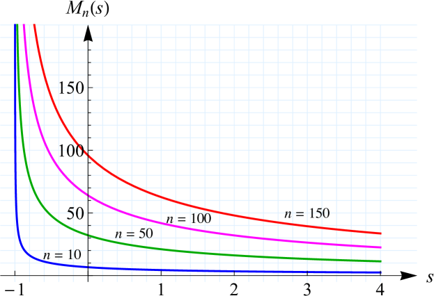
Note that we put (beta[s][[1]]=1), which is not important (see a comment in Section 2). The routine aZero computes all zeros of an orthogonal polynomial of degree as an increasing sequence. Graphics of for
and are displayed in Figure 1.
Figure 1. Best constants for and , when
There are several papers in which the authors give different estimates for the best constant for the generalized Laguerre weight function.
For example, Dörfler [20] determined certain lower and upper bounds for the best constant in the form
where is the first positive zero of the Bessel function of the first kind and order . For
it gives .
As an interesting result we mention a connection between the polynomials from Theorem 6.2 and the Pollaczek polynomials , defined by the recurrence relation [16, p. 84],
with and , in the form
(see [21, Lemma 1]). This choice of parameters in causes the corresponding Pollaczek polynomials to be no longer orthogonal. In that case for (see [21, Remark 3]).
More general problem was considered by Aptekarev, Draux, and Toulyakov [8] for the so-called co-recursive Pollaczek polynomials , defined by
(6.9)
with and , where and and are positive numbers with . They studied the measure of orthogonality of these polynomials outside the interval supporting the absolute continuous part of the measure of orthogonality of the corresponding non-perturbed system, i.e., the case , when (6.9) reduces to
with and , and the interval of orthogonality
In their interesting paper the authors obtained conditions on the parameters , and in order that the measure of orthogonality for the polynomials on the intervals
and possesses (i) no mass point, or (ii) a single mass point, or (iii) infinitely many (convergent) mass points. Moreover, they determined the explicit position of these mass points.
In an important particular case for extremal problems, when and , the polynomials reduce to the polynomials from Theorem 6.2. A discrete Markov-Bernstein inequality was also treated in [8]. Some results concerning bounds on the smallest zero of the polynomial and its asymptotic behavior were obtained in [7]. In [22] Draux used some numerical methods (qd algorithm, fixed point methods of increasing order, and Laguerre’s method) in order to obtain estimations for the polynomial zeros, as well as an improvement of the estimate for the best constants.
Recently, Nikolov and Shadrin [48] proved the following estimates for all and
where for the left-hand side inequality it is additionally assumed that . Nikolov and Shadrin also obtained bounds for the limit value in the form
The extremal problem (4.1) for the second derivative of polynomials was considered in [40] for the standard Laguerre weight function on . In that case we have , so that the matrix given by (4.7) of order becomes
(6.10)
and system of equation (4.8) can be written in the form
Introducing , it is easy to see that
so that we get the inverse matrix of as a triangular and tridiagonal matrix
Finally, for the matrix we get
the following five diagonal symmetric matrix of order ,
Thus, using the minimal eigenvalue of the matrix , we obtain the best constant
. The best constants for , , and are presented in Table 2, rounded to ten decimal digits to save space.
In a similar way, we can also calculate the best constants for each . The corresponding numerical values for the best constants
for are also presented in Table 2.
Table 2. Best constants for , , and , when
Remark 6.4.
The last problem can be connected
with extremal problems of Wirtinger’s type (see Milovanović et al.
[46, p. 578], as well as Mitrinović [47, p. 150], Fan et al. [24], G. V. Milovanović and I. Ž. Milovanović [44]).
For and we have the exact values:
Note that and .
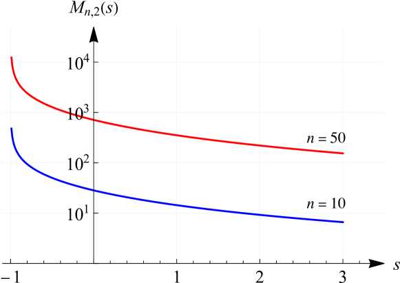
Figure 2 shows graphics of the best constants
for and in -scale.
Figure 2. Best constants in -scale for and , when
7. Extremal Problem With the Jacobi Weight
In this section we consider Markov’s extremal problem (4.1) on the space , where . The
inner product is defined by (1.6), and we use the expansion (3.10), jointly with the formulas (3.6) and (3.11)–(3.13), in order to determine the elements of the matrix . So we have
where
is given by (3.6), and the leading coefficients of the orthonormal Jacobi polynomials are given by (3.13) for and by (3.12) for .
The following commands in Mathematica 12.3 provide these calculations, where the upper triangular matrix (4.7) is denoted by Ank[n,k,al,be],
as well as the matrices and/or
, that appear in Theorem 4.1.
For example, for given , and (Chebyshev weight of the third kind), the matrix , its minimal eigenvalue and the best constant can be also obtained by the following commands:
In the general case, is a symmetric five-diagonal matrix.
Remark 7.1.
For the five-diagonal symmetric matrix of order (Chebyshev case of the third kind), one can prove that
and
In the Chebyshev case of the fourth kind , the all elements are the same as the previous ones, except which have only opposite sign of the previous ones.
In the sequel we consider Markov’s extremal problems only with the Gegenbauer weight for . The elements of the first sub-diagonals in the corresponding symmetric matrix
are equal to zero and the eigenvalue problem for such a matrix can be reduced to two eigenvalues problems for tridiagonal matrices (cf. [40]).
Thus, we now consider the matrix
(7.1)
and prove the following auxiliary result which is related to a decomposition of determinants of this type of matrices222For some more general cases, with the even weight function on a symmetric interval , see [40] and [46, pp. 579–582]..
Lemma 7.2.
Let and be symmetric tridiagonal matrices given by
(7.2)
and
(7.3)
Then
(7.4)
Proof.
For the determinant of the matrix , given by (7.1), we use the Laplace expansion.
Let first be even . Expanding by columns numbered , , , , one finds that only one non-zero contribution results, namely from the minor and cominor pair
In this way, one immediately obtains the relation (7.4).
Similarly, Laplace expansion by columns gives the result for odd . ∎
where is an identity matrix of order . In this way, the eigenvalue problem for reduces to two eigenvalue problems for matrices of lower orders and the second part of Theorem 4.1 gives the following result:
Theorem 7.3.
Let , , and the tridiagonal matrices and be given as in Lemma 7.2.
Then the best constant in Markov’s extremal problem is
(7.5)
where and are the minimal eigenvalues of matrices and , respectively.
In particular, we consider now three different important cases (see [40]):
1. Legendre case . In this case, using the elements of the matrix , with only two non-zero diagonals
and
we get the elements of the matrix in (7.1) as
, i.e.,
and
Since the elements are negative, in order to reduce the eigenvalue problems with the matrices (7.2) and (7.3)
in the way we did before, we introduce
and
In fact, in this way we consider the matrices , and , which have their eigenvalues only with opposite signs from those for the original matrices , and , respectively. But now, the matrices and can be interpreted as Jacobi matrices for certain measures and we can, as before, to apply the efficient Mathematica package OrthogonalPolynomials (see [17, 42]) for calculating the best constants , given by (7.5).
2. Chebyshev case of the first kind . In a similar way we obtain
and
so that the corresponding recurrence coefficients are
and
3. Chebyshev case of the second kind . Here,
we have
and
so that
and
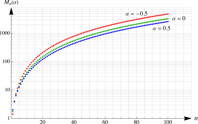
Figure 3 shows graphics of the best constants
in (7.5) for in -scale for .
Figure 3. Best constants
in (7.5) for in -scale, when
Remark 7.4.
In the previous cases , , the expression (7.5) can be written as
Recently Nikolov and Shadrin [49] (see also [4, 3, 23])
have been considered the best constant in (7.5). Taking , , and , they derived explicit lower and upper bounds for for each ,
and
In [7] Aptekarev, Draux and Kalyagin discussed the asymptotics of in (7.5) when , and proved that
the best constant has the asymptotics
(7.6)
where is the smallest zero of the Bessel function .
Recently, Aptekarev, Draux, Kalyagin, and Tulyakov [9]
have considered the asymptotics of the best constant
in the general extremal problem in the space , with the Jacobi weight function on .
Let the parameters of the Jacobi weight function satisfy the restriction . Then, for the best constant
we have the asymptotics
(7.7)
where is the smallest zero of the Bessel function .
Evidently for , (7.7) reduces to (7.6). In order to get the previous generalization, the authors needed to prove that linearly independent particular solutions of differential equations which satisfy the boundary conditions at the initial values of the discrete variable of a finite difference problem indeed are close to the particular solutions of the finite difference problem.
Remark 7.7.
The authors of [9] pointed out that the most surprising result for them is the appearance of the restriction on the parameters . Their comment was that they cannot prove or disapprove its necessity; however, they have to admit that this restriction is unavoidable in their proof strategy of Theorem 7.6.
Recently Totik [55] has proved Theorem 7.6, without the previous restriction on the parameters . Actually he proved a more general result, giving the exact asymptotic Markov constant for generalized Jacobi weight on several intervals.
Remark 7.8.
Using Sobolev spaces with continuous and discrete coherent pairs of weights, Aptekarev, Draux, and Tulyakov [10] studied the asymptotic behavior of the best constants in Markov-Bernstein inequalities with classical weighted integral norms.
8. Markov’s Extremal Problems on Some Restricted Classes of Polynomials
In this section we only mention Markov’s extremal problems
on for some restricted classes of polynomials , i.e.,
(8.1)
Usually we can restrict zeros of polynomials or their coefficients. In this way, the corresponding best constant can be improved. For such kind of extremal problems in uniform norm see
Milovanović at al. [46, pp. 624–643].
In 1981 Varma [57] investigated the problem of determining the best constant in
the inequality
on the space ,
with the generalized Laguerre weight function ,
for polynomials , where
(8.2)
For such polynomials and , he proved that
with equality for , and for
The ranges and are not covered by Varma’s results.
After attempts by several authors (cf.
[41, pp. 417–419]), this gap was filled by Milovanović [39], who determined the best constant
for all .
As we can see, the best constant is a continuous non-increasing function in . The sequences is a decreasing, and converges to
Otherwise, a few first terms of this sequences are
It is clear that , because , but for the constants for different are the same. Notice, that for the same expression holds for each , i.e.,
. Also, it is interesting to mention that in the limit case when , the best constant becomes the constant for each .
The corresponding extremal problems for higher derivatives are also investigated, as well as for other weight functions
(for details see [40, 45] and [46, pp. 644–664]).
Acknowledgement.
The work was supported in part by the Serbian Academy of Sciences and Arts (-96).
References
[1]
R. P. Agarwal and G. V. Milovanović,
A characterization of the classical orthogonal polynomials,
In: Progress in Approximation Theory (P. Nevai, A. Pinkus, eds.), pp. 1–4, Academic Press, New York, 1991
[2]
R. P. Agarwal and G. V. Milovanović,
Extremal problems, inequalities, and classical orthogonal polynomials,
Appl. Math. Comput. 128 (2002), 151–166.
[3]
D. Aleksov and G. Nikolov,
Markov inequality with the Gegenbauer weight,
J. Approx. Theory 225 (2018), 224–241.
[4]
D. Aleksov, G. Nikolov and A. Shadrin,
On the Markov inequality in the norm with the
Gegenbauer weight, J. Approx. Theory 208 (2016),
9–20.
[5]
W. A. Al-Salam and T. S. Chihara,
Another characterization of the classical orthogonal
polynomials, SIAM J. Math. Anal. 3 (1972), 65–70.
[6]
G. E. Andrews, R. Askey and R. Roy,
Special Functions,
Encyclopedia of Mathematics and its Applications, Vol. 71,
Cambridge University Press, Cambridge, 1999.
[7]
A. I. Aptekarev, A. Dro and V. A. Kalyagin,
On the asymptotics of exact constants in
Markov-Bernstein inequalities in integral metrics with classical weight,
Uspekhi Mat. Nauk 55 (2000), no. 1(331), 173–174
(Russian)
[8]
A. I. Aptekarev, A. Draux and D. Toulyakov,
Discrete spectra of certain co-recursive
Pollaczek polynomials and its applications,
Comput. Methods Funct. Theory 2 (2002), 519–537.
[9]
A. I. Aptekarev, A. Draux, V. A. Kalyagin and D. N. Tulyakov,
Asymptotics of sharp constants of Markov-Bernstein inequalities in integral norm with Jacobi weight.
Proc. Amer. Math. Soc. 143 (9) (2015), 3847–3862.
[10]
A. I. Aptekarev, A. Draux and D. N. Tulyakov,
On asymptotics of the sharp constants of the
Markov-Bernstein inequalities for the Sobolev spaces.
Lobachevskii J. Math. 39 (5) (2018), 609–622.
[11]
S. N. Bernstein,
Sur l’ordre de la meilleur approximation des fonctions continues par des polynômes de degré donné,
Memoire d el’Académie Royal de Belgique 4 (2) (1912),
1–103.
[12]
B. D. Bojanov,
An extension of the Markov inequality,
J. Approx. Theory 35 (1982), 181–190.
[13]
P. B. Borwein and T. Erdélyi,
Polynomials and Polynomial Inequalities.
Springer Verlag, New York, 1995.
[14]
A. Böttcher and P. Dörfler,
Weighted Markov-type inequalities, norms of Volterra operators, and zeros of Bessel functions,
Math. Nachr. 283 (2010), 40–57.
[15]
A. Böttcher and P. Dörfler,
On the best constants in Markov-type inequalities involving Laguerre norms with different weights,
Monatsh. Math. 161 (4) (2010), 357–367.
[16]
T. S. Chihara,
An Introduction to Orthogonal Polynomials.
Gordon and Breach Science Publishers, New York-London-Paris,
1978.
[17]
A. S. Cvetković and G. V. Milovanović,
The Mathematica package
“OrthogonalPolynomials”,
Facta Univ. Ser. Math. Inform. 19 (2004),
17–36.
[18]
P. Dörfler,
New inequalities of Markov type,
SIAM J. Math. Anal. 18 (1987), 490–494.
[19]
P. Dörfler,
A Markov type inequality for higher derivatives of
polynomials,
Monatsh. Math. 109 (1990), 113–122.
[20]
P. Dörfler,
Über die bestmögliche Konstante in
Markov-Ungleichungen mit Laguerre-Gewicht,
Österreich. Akad. Wiss. Math.-Natur. Kl. Sitzungsber. II
200 (1-10) (1991), 13–20.
[21]
P. Dörfler,
Asymptotics of the best constant in a certain Markov-type inequality,
J. Approx. Theory 114 (2002), 84–97.
[22]
A. Draux,
Improvement of the formal and numerical estimation of the constant in some Markov-Bernstein inequalities,
Numer. Algorithms 24 (2000), 31–58.
[23]
A. Draux and V. Kaliaguine,
Markov-Bernstein inequalities for
generalized Gegenbauer weight,
East J. Approx. 12 (2006), 1–23.
[24]
K. Fan, O. Taussky and J. Todd,
Discrete analogs of inequalities of Wirtinger,
59 (1955), 73–90.
[25]
W. Gautschi,
Orthogonal Polynomials: Computation and Approximation, Clarendon Press, Oxford, 2004.
[26]
P. Yu. Glazyrina,
Markov-Nikol’skiĭ inequality for the spaces , on a segment,
Proc. Steklov Inst. Math. 31 (2005), S104–S116.
[27]
P. Yu. Glazyrina,
The Markov brothers’ inequality in the space on an interval,
Mat. Zametki 78 (2005), 59–65.
[28]
P. Yu. Glazyrina,
The sharp Markov-Nikol’skiĭ inequality for algebraic polynomials in the spaces and on an interval, Mat. Zametki 84 (2008), 3–22.
[29]
A. Guessab,
Some weighted polynomial inequalities in -norm,
J. Approx. Theory 79 (1994), 125–133.
[30]
A. Guessab,
Weighted Markoff type inequality for classical weights,
Acta Math. Hung. 66 (1995), 155–162.
[31]
A. Guessab and G. V. Milovanović,
Weighted -analogues of Bernstein’s inequality and classical orthogonal polynomials,
J. Math. Anal. Appl. 82 (1994), 244–249.
[32]
A. Guessab and G. V. Milovanović,
Extremal problems of Markov’s type for some differential operators,
Rocky Mountain J. Math. 24 (1994), 1431–1438.
[33]
S. V. Konjagin,
Estimation of the derivatives of polynomials,
Dokl. Akad. Nauk SSSR 243 (5) (1978), 1116–1118 (Russian).
[34]
A. A. Markov,
On a problem of D. I. Mendeleev,
Zapishi Imp. Akad. Nauk 62
(1889), 1–24 (Russian).
[35]
V. A. Markov,
On functions deviating least from zero in a given interval,
Izv. Akad. Nauk St. Petersburg, St. Petersburg, 1892,
pp. 1–110 (Russian).
[36]
V. A. Markov,
Über Polynome die in einem gegebenen Intervalle möglichst wenig von null abweichen,
Math. Annalen 77 (1916), 213–258.
[37]
G. Mastroianni and G. V. Milovanović,
Interpolation Processes – Basic Theory and Applications, Springer-Verlag,
Berlin – Heidelberg – New York, 2008.
[38]
D. Mendeleev,
Investigation of aqueous solutions based on specific gravity, St. Petersburg, 1887 (Russian).
[39]
G. V. Milovanović,
An extremal problem for polynomials with nonnegative coefficients,
Proc. Amer. Math. Soc. 94 (1985), 423–426.
[40]
G. V. Milovanović,
Various extremal problems of Markov’s type for algebraic polynomials,
Facta Univ. Ser. Math. Inform. 2 (1987), 7–28.
[41]
G. V. Milovanović,
Extremal problems for restricted polynomial classes in norm,
In: Approximation Theory: In Memory of A. K. Varma (N. K. Govil, R. N. Mohapatra, Z. Nashed, A. Sharma and J. Szabados, eds.), pp. 405–432, Marcel Dekker, New York, 1998.
[42]
G. V. Milovanović and A. S. Cvetković,
Special classes of orthogonal polynomials and corresponding quadratures of Gaussian type,
Math. Balkanica (N.S.) 26 (2012), 169–184.
[43]
G. V. Milovanović and R. Ž. Djordjević,
Linear Algebra, Faculty of Electronic Engineering,
Niš, 2004 (Serbian).
[44]
G. V. Milovanović and I. Ž.
Milovanović,
On discrete inequalities of Wirtinger’s type,
J. Math. Anal. Appl. 88 (1982), 378–387.
[45]
G. V. Milovanović and M. S. Petković,
Extremal problems for Lorentz classes of nonnegative polynomials in metric with Jacobi weight,
Proc. Amer. Math. Soc. 102
(1988), 283–289.
[46]
G. V. Milovanović, D. S. Mitrinović and Th. M. Rassias,
Topics in Polynomials: Extremal Problems, Inequalities, Zeros, World Scientific,
Singapore – New Jersey – London – Hong Kong, 1994.
[47]
D. S. Mitrinović (in cooperation with P. M. Vasić),
Analytic Inequalities,
Die Grundlehren der mathematischen Wissenschaften, Band 165,
Springer-Verlag, New York-Berlin, 1970.
[48]
G. Nikolov and A. Shadrin,
On the Markov inequality with Laguerre weight,
In: Progress in Approximation Theory and Applicable Complex
Analysis: In Memory of Q. I. Rahman (N. K. Govil, R. Mohapatra, M. A. Qazi and G. Schmeisser, eds.), pp. 1–17, Springer, Cham, 2017.
[49]
G. Nikolov and A. Shadrin,
On the Markov inequality in the -norm with the
Gegenbauer weight, Constr. Approx. 49
(2019), 1–27.
[50]
Q. I. Rahman and G. Schmiesser,
Analytic Theory of Polynomials, London Mathematical Society Monographs New Series, 26, Clarendon Press,
Oxford, 2002.
[51]
E. Schmidt,
Über die nebst ihren Ableitungen orthogonalen
Polynomensysteme und das zugehörige Extremum,
Math. Ann. 119 (1944), 165–204.
[52]
L. F. Shampine,
Asymptotic Inequalities of Markoff Type, Ph.
Thesis, California Institute of Technology,
Pasadena, 1964.
[53]
L. F. Shampine,
Some Markoff inequalities,
J. Res. Nat. Bur. Standards 69B (1965), 155–158.
[54]
I. E. Simonov,
Sharp Markov brothers type inequality in the spaces and on a closed interval,
Proc. Steklov Inst. Math. 277 (2012), S161–S170.
[55]
V. Totik,
Sharp constants in weighted -Markov inequalities,
Proc. Amer. Math. Soc. 147 (1) (2019), 153–166.
[56]
P. Turán, Remark on a theorem of Erhard Schmidt,
Mathematica (Cluj) 2 (25)
(1960), 373–378.
[57]
A. K. Varma,
Derivatives of polynomials with positive coefficients,
Proc. Amer. Math. Soc. 83 (1981), 107–112.
[58]
E. V. Voronovskaja,
The Functional Method and its Applications,
Trans. Math. Monographs
28, Amer. Math. Soc., Providence, 1970.