Determination of the spectroscopic parameters of beauty-partners of $T_{cc}$ from QCD

Abstract

Motivated by the recent discovery of a new tetra-quark $T_{cc}^{+}$ state with two charm quarks and two light quarks by LHCb collaboration, we calculate the spectroscopic parameters, namely, the mass and residues of beauty partners of $T_{cc}^{+}$ within QCD sum rules. The obtained results are compared with the predictions of different approaches in the literature.

I Introduction

The study of hadron spectroscopy represents a promising way to understand the inner structure of the hadrons. The quantum chromodynamics (QCD) theory allows the existence of multiquark states in a color singlet state. The first observation of such states, $X(3872)$, was achieved by BELLE collaboration [1]. Many multi-quarks states have been discovered up to now. The properties of such states have been widely analyzed by theorists and experimentalists (see review [2, 3, 4]).

All the discovered exotic hadrons have been achieved by analyzing their strong interactions. The measured decay widths lie in the domain of a few to a few hundred MeV. On the other hand, observing a long-lived exotic state that is stable with respect to the strong interaction would be exciting. The first candidates of such states are expected to be hadrons with two heavy quarks (Q) and two light antiquarks (q). Recently, LHCb collaboration has reported discovering such a state, namely tetraquark state $T_{cc}^{+}$ with two charm quarks and two light antiquarks in the $D^{0}D^{0}\pi^{+}$ spectrum [5, 6] with quantum numbers $J^{P}=1^{+}$. The observed decay width and the mass difference is .[5]

$$\begin{split}\delta m&=m_{T_{cc}^{+}}-(m_{D^{*+}}+m_{D^{0}})=-273\pm 61\pm 5^{+11}_{-14}~{}keV\\ \Gamma_{T_{cc}^{+}}&=410\pm 165\pm 43^{+18}_{-38}~{}keV~{}.\end{split}$$ (1)

This observation can stimulate studies of exotic hadrons in new ways. One of the possible interpretations of $T_{cc}^{+}$ is that it is a compact $DD^{*}$ hadronic state. This discovery inspires us to use the QCD sum rules approach to investigate the mass and residues of all the exotic $T_{bbqq}$ states, potentially to be observed in the near future, with quantum numbers $J^{P}=1^{+}$. In calculations, we also take into account the $SU(3)$ violation effects.

The paper is organized as follows. In Section II, we derive sum rules for the mass and residue of the possible bottomonium states. Section III is devoted to the numerical analysis of the obtained sum rules. This section also contains discussions and comparisons of our findings with the other approaches. And finally, we conclude our study.

II Mass sum rules for bottomonium states with $J^{P}=1^{+}$

Before deriving the sum rules, we present all the possible bottomonium states with quantum numbers $J^{P}=1^{+}$ (see Table  1.)

$T_{bb}$ States	Tetraquark Contents
$T_{bb}^{--}$	$B^{-}B^{*-}$
$T_{bb}^{-}$	$B^{0}B^{*-}$, $B^{-}B^{*0}$
$T_{bb}^{0}$	$B^{0}B^{*0}$
$T_{bb(s)}^{-}$	$B_{s}^{0}B^{*-}$, $B_{s}^{*0}B^{-}$
$T_{bb(s)}^{0}$	$B_{s}^{0}B^{*0}$, $B^{*0}B_{s}^{*0}$
$T_{bb(ss)}^{0}$	$B_{s}^{0}B_{s}^{*}$

Table 1: Possible states of $T_{bb}$ with $J^{P}=1^{+}$.

We choose the interpolating current for $T_{bb}$ state with quantum numbers $J^{P}=1^{+}$ as

$$j_{\mu}=(\bar{q_{1}}^{a}i\gamma_{5}Q_{1}^{a})(\bar{q_{2}}^{b}\gamma_{\mu}Q_{2}^{b})$$ (2)

where $a$ and $b$ are the color indices, $q_{1}(q_{2})$ is the light quark, and $Q_{1}(Q_{2})$ represents heavy quarks. The light and heavy quarks can either be the same or different.

To obtain the mass sum rules we consider the following correlation function,

$$\begin{split}\Pi_{\mu\nu}&=i\int d^{4}x\langle 0|T\big{(}j_{\mu}(x)j_{\nu}^{\dagger}(0)\big{)}|0\rangle\\ &=(-g_{\mu\nu}+\frac{p_{\mu}p_{\nu}}{p^{2}})\Pi_{1}+\frac{p_{\mu}p_{\nu}}{p^{2}}\Pi_{2}\end{split}$$ (3)

where $\Pi_{1}$ and $\Pi_{2}$ represent the invariant functions corresponding to transversal and longitudinal parts of the correlation function.

According to the QCD sum rules method, the correlation function is calculated in two different kinematical regions; in terms of hadrons and in the deep Euclidean region $p^{2}\rightarrow-\infty$ using the Operator product expansion(OPE). Matching these two representations and performing Borel transformation with respect to the variable $-p^{2}$ to suppress the contributions from the excited states and continuum as well as to enhance the ground state contribution, we get mass sum rules.

Now let us calculate the correlation function from the hadronic side first. The hadronic representation of the correlation function satisfies the dispersion relation,

$$\Pi_{i}=\int\frac{\rho_{i}(s)ds}{s-p^{2}}+\text{subtractions},$$ (4)

where $i=1(2)$ corresponds to $\Pi_{1}$ and $\Pi_{2}$ and $\rho_{i}(s)$ is the corresponding spectral density. Inserting a complete set of intermediate states with the same quantum numbers as the interpolating current $J^{P}=1^{+}$ and isolating the ground state contribution for the spectral density we get

$$\rho_{i}=\lambda_{i}^{2}\delta(s-m_{T}^{2})+...$$ (5)

where dots denotes the contribution from higher states. To obtain this spectral density, we used the standard definition

$$\langle 0|j_{\mu}|T_{QQ}(p)\rangle=\lambda\epsilon_{\mu}~{},$$ (6)

where $\lambda$, and $\epsilon_{\mu}$ are the decay constant, and vector polarization of $T_{QQ}$ bottomed state. Then we performed summation over spins of $T_{QQ}$ and separated the coefficient of the structure $g_{\mu\nu}-\frac{p_{\mu}p_{\nu}}{p^{2}}$.

As we already noted that the theoretical part of the correlation function is calculated in the deep Euclidean domain with the help of OPE. After simple calculations, we obtain the correlation function for $T_{bb}$ as follows: for case $Q_{1}=Q_{2}=Q$ and $q_{1}\neq q_{2}$:

$$\begin{split}\Pi_{\mu\nu}=i\int d^{4}xe^{ipx}\Bigg{\{}&Tr\big{[}S_{Q}^{ba^{\prime}}(x)\gamma_{5}S_{q_{1}}^{a^{\prime}a}(-x)\gamma_{5}S_{Q}^{ab^{\prime}}(x)\gamma_{\nu}S_{q_{2}}^{b^{\prime}}(-x)\gamma_{\mu}\big{]}\\ -&Tr\big{[}\gamma_{5}S_{Q_{1}}^{aa^{\prime}}(x)\gamma_{5}S_{Q_{1}}^{a^{\prime}a}(-x)\big{]}Tr\big{[}\gamma_{\mu}S_{Q}^{bb^{\prime}}(x)\gamma_{\nu}S_{q_{2}}^{b^{\prime}b}(-x)\big{]}\Bigg{\}}\end{split}$$ (7)

and for $Q_{1}=Q_{2}=Q$ and $q_{1}=q_{2}=q$ case:

$$\begin{split}\Pi_{\mu\nu}=i\int d^{4}xe^{ipx}\Bigg{\{}&Tr\big{[}\gamma_{5}S_{Q}^{ab^{\prime}}(x)\gamma_{\nu}S_{q}^{b^{\prime}a}(-x)\big{]}Tr\big{[}\gamma_{\mu}S_{Q}^{ba^{\prime}}(x)\gamma_{5}S_{q}^{ab}(-x)\big{]}\\ +&Tr[\gamma_{5}S_{Q}^{aa^{\prime}}(x)\gamma_{5}S_{q}^{a^{\prime}a}(-x)]Tr\big{[}\gamma_{\mu}S_{Q}^{bb^{\prime}}(x)\gamma_{\nu}S_{d}^{bb^{\prime}}(-x)\big{]}\\ -&Tr\big{[}S_{Q}^{ba^{\prime}}(x)\gamma_{5}S_{d}^{a^{\prime}a}(-x)\gamma_{5}S_{Q}^{ab^{\prime}}(x)\gamma_{\nu}S_{q}^{b^{\prime}b}(-x)\gamma_{\mu}\big{]}\\ -&Tr\big{[}S_{Q}^{bb^{\prime}}(x)\gamma_{\nu}S_{d}^{b^{\prime}a}(-x)\gamma_{5}S_{Q}^{aa^{\prime}}(x)\gamma_{5}S_{q}^{a^{\prime}b}(-x)\gamma_{\mu}\big{]}\Bigg{\}}\end{split}$$ (8)

The QCD sum rules are obtained by choosing the same Lorentz structures from both representations of the correlation function and then matching the coefficients of these structures. In our calculations, we choose the structure $g_{\mu\nu}$ since it only contains the contributions of spin-1 particles. From Eq. (7), it follows that light and heavy quark propagators are needed to calculate the correlation function. Light quark propagator in $x$-representation up to the first order of light quark mass is given as .[7, 8]

$$\begin{split}S_{q}^{ab}(x)&=\frac{i\not{x}\delta^{ab}}{2\pi^{2}x^{4}}-\frac{m_{q}}{4\pi^{2}x^{2}}\delta^{ab}-\frac{1}{12}\langle\bar{q}q\rangle\delta^{ab}+\frac{g_{s}G^{n}_{\mu\nu}(\frac{\lambda^{n}}{2})^{ab}}{32\pi^{2}x^{2}}(i\sigma^{\mu\nu}\not{x}+i\not{x}\sigma^{\mu\nu})+im_{q}\frac{\bar{q}q}{48}\not{x}\delta^{ab}\\ &+\frac{1}{192}m_{0}^{2}\langle\bar{q}q\rangle x^{2}\delta^{ab}-i\frac{m_{q}}{1152}m_{0}^{2}\langle\bar{q}q\rangle x^{2}\not{x}\delta^{ab}-\frac{4\pi}{3^{9}2^{10}}\langle\bar{q}q\rangle\langle\alpha_{s}G^{2}\rangle x^{2}\delta^{ab}+...\end{split}$$ (9)

Besides, the heavy-Quark propagator in x-representation is (see for example [9]).

$$\begin{split}S_{Q}^{ab}(x)&=\frac{m_{Q}^{2}\delta^{ab}}{(2\pi^{2})}\bigg{\{}i\not{x}\frac{K_{2}(m_{Q}\sqrt{-x^{2}})}{(\sqrt{-x^{2}})^{2}}+\frac{K_{1}(m_{Q}\sqrt{-x^{2}})}{\sqrt{-x^{2}}}\bigg{\}}\\ &-\frac{m_{Q}g_{s}G^{n}_{\mu\nu}(\frac{\lambda^{n}}{2})^{ab}}{8(2\pi)^{2}}\bigg{\{}i[\sigma^{\mu\nu}\not{x}+\not{x}\sigma^{\mu\nu}]\frac{K_{1}(m_{Q}\sqrt{-x^{2}})}{\sqrt{-x^{2}}}+2\sigma^{\mu\nu}K_{0}\bigg{\}}\\ &-\frac{\delta^{ab}\langle g_{s}^{2}G^{2}\rangle}{576(2\pi)^{2}}\bigg{\{}(i\not{x}m_{Q}-6)\frac{K_{1}(m_{Q}\sqrt{-x^{2}})}{\sqrt{-x^{2}}}(-x^{2})+m_{Q}(x^{2})^{2}\frac{K_{2}(m_{Q}\sqrt{-x^{2}})}{(\sqrt{-x^{2}})^{2}}\bigg{\}}\end{split}$$ (10)

where $K_{i}$ are the modified Bessel functions of the second kind.

Using the Eqs. (9) and (10) for the light and heavy quark propagators, after lengthy calculation we can find the spectral density $\rho_{1}$. The expressions of the spectral density are presented in Appendix.

Matching the expressions of spectral density $\rho_{1}(s)$ from hadronic and OPE parts and performing Borel transformation with respect to variable $-p^{2}$ to suppress the continuum and higher states as well as enhancing the contribution of the ground state by using the quark-hadron duality, we get the sum rules for the spectroscopic parameters (mass and residue) of the considered $T_{bb}$ meson:

$$\lambda^{2}e^{-m_{T}^{2}/M^{2}}=\int^{s_{0}}_{s_{min}}ds\rho_{1}(s)e^{-s/M^{2}}$$ (11)

where $s_{min}=(m_{Q_{1}}+m_{Q_{2}}+m_{q_{1}}+m_{q_{2}})^{2}$, $M^{2}$ and $s_{0}$ are the Borel mass parameter square and continuum threshold respectively. Getting derivative with respect to $(-1/M^{2})$ and dividing the obtained result to Eq. $\eqref{eq:9}$ we get the desired sum rule for the mass of $T_{bb}$

$$m_{T}^{2}=\frac{\int^{s_{0}}_{s_{min}}s\rho_{1}(s)e^{-s/M^{2}}ds}{\int_{s_{min}}^{s_{0}}\rho_{1}(s)e^{-s/M^{2}}ds}$$ (12)

Moreover, once the $m_{T}^{2}$ is obtained from Eq. (12), we can obtain the residue by putting it into the Eq. (11).

At the end of this section, we would like to note that next to leading order (NLO), perturbative corrections to the correlation function for tetraquark systems with two heavy quarks have been calculated in ,[10] and it is obtained that the radiative corrections are quite small. Similarly, NLO corrections to the correlation function for the considered states are also expected to be small, and hence we neglected them in our calculations.

III Numerical Analysis

Having derived the expressions for the mass and residue for $T_{bb}$, we present the numerical results of these quantities in this section. The values of the input parameters used in our calculations are depicted in Table  2. For the heavy quark masses, we used their $\overline{MS}$ values.

Parameters	Value
$\overline{m}_{s}(1~{}GeV)$	$0.114\pm 0.021~{}GeV$ [11]
$\overline{m}_{b}(\overline{m}_{b})$	$4.18\pm 0.03~{}GeV$ [11]
$m_{K}$	$0.497~{}GeV$ [11]
$\langle\bar{q}q\rangle$	$-(0.245)^{3}~{}GeV^{3}$ [11]
$\langle\bar{s}s\rangle$	$(0.8\pm 0.2)~{}\langle\bar{q}q\rangle~{}GeV^{3}$  [12]
$m_{0}^{2}$	$(0.8\pm 0.2)~{}GeV^{2}$ [13]
$\langle\frac{\alpha_{s}G^{2}}{\pi}\rangle$	$(0.012^{+0.006}_{-0.0012})~{}GeV^{4}$  [14],

Table 2: The values of the input parameters used in our calculations.

The Borel mass parameters, $M^{2}$, and continuum threshold, $s_{0}$, are the auxiliary parameters of the sum rules. Hence, physical quantities are expected to be independent of these parameters. For this purpose, we need to find the “working regions” of these parameters where measurable quantities are insensitive to the variation of them. The upper bound of $M^{2}$ is determined from the condition that the higher states and continuum contributions should be suppressed compared to the total result, i.e., the dominance of pole contribution. The pole contribution (PC) is defined as

$$PC(s_{0},M^{2})=\frac{\int_{s_{min}}^{s_{max}}\rho_{1}(s)e^{-s/M^{2}}ds}{\int_{s_{min}}^{\infty}\rho_{1}(s)e^{-s/M^{2}}ds}$$ (13)

We require that the pole contribution constitute more than $50\%$ of the total result. The minimum value of the $M^{2}$ is obtained from the requirement that the operator product expansion is convergent. For this goal, we consider the following quantity

$$\mathcal{D}(n)=\frac{\int_{s_{min}}^{s_{0}}\rho_{1}^{(n)}(s)e^{-s/M^{2}}ds}{\int_{s_{min}}^{s_{0}}\rho_{1}(s)e^{-s/M^{2}}ds}$$ (14)

where $\rho_{1}^{(n)}$ corresponds to the spectral density describing the contribution of the condensate of dimension $n$. We demand that the contribution of condensate with maximum dimension in sum rules should be less than, say, $5\%$ of the total result. The minimum value of $M^{2}$ is determined from the condition that the continuum and higher state contributions should be suppressed compared to the total result. Besides, the upper bound of $M^{2}$ is obtained from the requirement the operator product expansion should be convergent, i.e., the power corrections should be suppressed with respect to the total result.

States	$M^{2}(GeV^{2})$	$s_{0}(GeV^{2})$	mass(GeV)	$\lambda^{2}(GeV^{10})$	Pole contribution $(\%)$
$BB^{*}$	$10-20$	$115-120$	$10.3\pm 0.1$	$0.030\pm 0.008$	$64-38$
$B_{s}B^{*}$	$10-20$	$120-125$	$10.4\pm 0.1$	$0.05\pm 0.01$	$68-38$
$BB_{s}^{*}$	$10-20$	$120-125$	$10.4\pm 0.1$	$0.05\pm 0.01$	$68-38$
$B_{s}B_{s}^{*}$	$10-20$	$125-130$	$10.7\pm 0.12$	$0.07\pm 0.02$	$72-42$

Table 3: The working regions of $M^{2}$ and $s_{0}$ as well as the value of residues for the considered states.

The threshold parameter $s_{0}$ is determined via the minimized variation of the $T_{bb}$ mass with respect to the variation of $M^{2}$. Considering these restrictions, one can determine the $s_{0}$ and $M^{2}$ for $T_{bb}$ states. Our numerical analysis shows that the conditions mentioned above are satisfied in the regions of $M^{2}$ and $s_{0}$ presented in Table  3. In this Table, we also present the pole contribution.

States	$BB^{*}(10604)$	$B_{s}B^{*}(10692)$	$BB_{s}^{*}(10695)$	$B_{s}B_{s}^{*}(10782)$
This Study	-304	-291.5	-295.1	-82
[15]	-215	—	—	—
[16]	-121	-48	-48	—
[17]	-133	-47	NB	NB
[18]	-116	-21	-21	NB
[19]	-464	—	—	—
[20]	-404	—	—	—
[21]	-224	-120	-123	—
[22]	-6	$\sim 0$	-2.1	$\sim 0$
[23]	-150	—	—	—
[24]	-35	—	—	—
[25]	-120.9	—	—	—
[26]	-317.6	—	—	—
[27]	-54	—	—	—
[28]	-102	NB	NB	NB
[29]	-173	-59	-59	—
[30]	NB	NB	NB	—
[31]	-145	-42	—	—
[32]	-278	-49	-49	NB
[33]	-189	-98	-98	—
[34]	-143	-87	-87	—
[35]	-128	—	—	—
[36]	-167	—	—	—

Table 4: Theoretical results for the binding energy (in $\rm{MeV}$ units) of $T_{bb}$ states predicted by different approaches are presented. Here, NB stands for the no-bound state. The values inside the parenthesis correspond to the threshold values of the corresponding meson-meson states.

In Fig. 1, we presented the dependency of the mass of $T_{bb}$ state on Borel mass parameters $M^{2}$ at the fixed values of $s_{0}$. From this figure, we get $m=10300\pm 100$ MeV for the $T_{bb}$ state. Performing similar numerical analysis for the other $T_{bb}$ states such as $B_{s}B^{*}(BB_{s}^{*})$ and $B_{s}B_{s}^{*}$, we obtained the residues and mass values of the corresponding states that are presented in Table  3. In the determination of the mass, we take into account the uncertainties coming from input parameters as well as from the variation of $M^{2}$ and $s_{0}$.

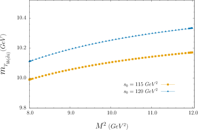
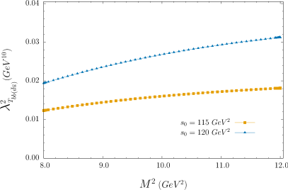
Figure 1: The dependencies of mass and residue of the $T_{bb}$ state on Borel mass square at the fixed values of $s_{0}$.

In Table 4, we present our theoretical results for the binding energy (in MeV) of $T_{bb}$ states. Moreover, for completeness in this Table, we also present the binding energy predicted by the other approaches. From the comparison, we observe that our predictions on the binding energy of $T_{bb}$ are larger than the results of other approaches, especially for $B_{s}B^{*}$, $BB_{s}^{*}$, and $B_{s}B_{s}^{*}$ states. On the other hand, for the $BB^{*}$ state, our finding on the mass difference is less than the predictions obtained in [19, 20, 26] and larger than the other results. This circumstance hopefully can be clarified in future experiments.

Finally, we would like to make the following remark. To derive the sum rules, we used a simple one-pole approximation. However, for the case of a multiquark state, the physical side of the sum rules in principle can receive contributions from two-particle hadronic states at least. This point was first raised in [37, 38]. The multiquark state can decay into kinematically allowed states; hence, we should take into account the decay width of multiquark states. Once we do that, the quark propagator should be replaced in the following way.

$$\frac{1}{m^{2}-p^{2}}\rightarrow\frac{1}{m^{2}-p^{2}-i\Gamma\sqrt{p^{2}}}~{},$$ (15)

where $\Gamma$ is the decay width of $T_{bb}$ state. For the observed $T_{cc}^{+}$ state, the width was measured as $\Gamma_{T_{cc}}\sim 400~{}keV$, which was smaller than the mass of $T_{cc}^{+}$. We expect a similar case for the $T_{bb}$ state. In this situation, one can safely neglect the contributions of two hadronic states in the phenomenological part of the correlation function.

IV Conclusion

Motivated by the recent observation of double charmed tetraquark $T_{cc}^{+}$ by LHCb collaboration, we investigated the mass spectrum and residues of the possible doubly bottomed tetraquark states with quantum numbers $J^{P}=1^{+}$ within the QCD sum rules method. We compared our results with the findings of other theoretical approaches. Future LHCb experiments will hopefully hunt the states considered in this study.

*

Appendix A The expression of the spectral densities

In this Appendix, we present the expressions of the spectral density for the $BB^{*}$ system with the quantum number $J^{P}=1^{+}$. The spectral density contains the perturbative contribution, the quark, and gluon condensate terms, quark-gluon mixed terms, four quark condensates, and dimension eight, nine terms. Their expressions are;

$$\rho^{(pert)} = {1\over(3\times 2^{14})\pi^{6}}\int_{\alpha_{min}}^{\alpha_{max}}{d\alpha\over\alpha^{3}}\int_{\beta_{min}}^{\beta_{max}}{d\beta\over\beta^{3}}\Big{[}(\alpha+\beta)m_{b}^{2}-\alpha\beta s\Big{]}^{2}$$ (16)

$$\times \Big{\{}(1-\beta)\beta m_{b}^{3}\big{[}(8+29\beta(1+\beta))m_{b}-120\beta(m_{d}+\beta m_{d}+2m_{u})\big{]}$$

$$- \alpha^{4}(29m_{b}^{2}-33\beta s)(m_{b}^{2}-\beta s)+2\alpha m_{b}\big{\{}m_{b}\big{[}(4+21\beta-58\beta^{3})m_{b}^{2}$$

$$+ 12\beta(33-32\beta)m_{d}m_{u}-60\beta m_{b}(m_{d}-3\beta^{2}m_{d}+2m_{u}-4\beta m_{u})\big{]}$$

$$- (1-\beta)\beta\big{[}(4+31\beta(1+\beta))m_{b}-60\beta(m_{d}+\beta m_{d}+2m_{u})\big{]}s\big{\}}$$

$$- 2\alpha^{3}\beta(58m_{b}^{4}-60m_{b}^{3}m_{d}-93\beta m_{b}^{2}s+60\beta m_{b}m_{d}s+33\beta^{2}s^{2})$$

$$+ 3\alpha^{2}\big{\{}(7-58\beta^{2})m_{b}^{4}+40\beta m_{b}^{3}(3\beta m_{d}+2m_{u})-80\beta^{2}m_{b}(\beta m_{d}+m_{u})s$$

$$- 2\beta m_{b}^{2}(128m_{d}m_{u}+9s-31\beta^{2}s)-\beta^{2}s\big{[}8m_{d}m_{u}-11(1-\beta^{2})s\big{]}\big{\}}\Big{\}}$$

$$\rho^{(\langle\bar{u}u\rangle)} = -{\langle\bar{u}u\rangle\over 2^{10}\pi^{4}}\int_{\alpha_{min}}^{\alpha_{max}}{d\alpha\over\alpha(1-\alpha)}\big{[}m_{b}^{2}-(1-\alpha)\alpha s\big{]}$$ (17)

$$\times \big{[}20(1-\alpha)m_{b}m_{d}m_{u}-m_{b}^{2}(2m_{d}+11m_{u})+(1-\alpha)\alpha(2m_{d}+11m_{u})s\big{]}$$

$$- {\langle\bar{u}u\rangle\over 2^{10}\pi^{4}}\int_{\alpha_{min}}^{\alpha_{max}}{d\alpha\over\alpha^{2}}\int_{\beta_{min}}^{\beta_{max}}{d\beta\over\beta}\big{[}(\alpha+\beta)m_{b}^{2}-\alpha\beta s\big{]}$$

$$\times \Big{\{}m_{b}\big{\{}4m_{b}\big{[}5(\alpha+\beta)m_{b}-11\alpha m_{d}\big{]}+\alpha\big{[}9(\alpha+\beta)m_{b}-20\beta m_{d}\big{]}m_{u}\big{\}}$$

$$- \alpha\beta(20m_{b}+11\alpha m_{u})s\Big{\}}$$

$$\rho^{(\langle\bar{d}d\rangle)} = {\langle\bar{d}d\rangle\over 2^{10}\pi^{4}}\int_{\alpha_{min}}^{\alpha_{max}}{d\alpha\over\alpha(1-\alpha)}\big{[}m_{b}^{2}-(1-\alpha)\alpha s\big{]}\Big{\{}m_{b}\big{\{}11m_{b}m_{d}$$ (18)

$$+ 2\big{[}m_{b}-10(1-\alpha)m_{d}\big{]}m_{u}\big{\}}-(1-\alpha)\alpha(11m_{d}+2m_{u})s)$$

$$- {\langle\bar{d}d\rangle\over 2^{10}\pi^{4}}\int_{\alpha_{min}}^{\alpha_{max}}{d\alpha\over\alpha^{2}}\int_{\beta_{min}}^{\beta_{max}}{d\beta\over\beta}\big{[}(\alpha+\beta)m_{b}^{2}-\alpha\beta s\big{]}\Big{\{}m_{b}^{2}\big{\{}(\alpha+\beta)$$

$$\times \big{[}20(\alpha+\beta)m_{b}+9\alpha m_{d}\big{]}-44\alpha m_{u}\big{\}}-\alpha\beta\big{[}20(\alpha+\beta)m_{b}+11\alpha m_{d}\big{]}s\Big{\}}$$

$$\rho^{(\langle g^{2}G^{2}\rangle)} = {\langle g^{2}G^{2}\rangle\over(3\times 2^{15})m_{b}\pi^{6}}\int_{\alpha_{min}}^{\alpha_{max}}{d\alpha\over\alpha(1-\alpha)}\Big{\{}\big{[}m_{b}^{2}-(1-\alpha)\alpha s\big{]}$$ (19)

$$\times \Big{(}m_{b}\big{[}33m_{b}^{2}+80(1-\alpha)m_{d}m_{u}-20m_{b}(m_{d}+m_{u})\big{]}$$

$$- (1-\alpha)\alpha\big{[}33m_{b}-20(m_{d}+m_{u})\big{]}s\Big{)}\Big{\}}$$

$$- {\langle g^{2}G^{2}\rangle\over(3\times 2^{16})m_{b}\pi^{6}}\int_{\alpha_{min}}^{\alpha_{max}}{d\alpha\over\alpha^{2}}\int_{\beta_{min}}^{\beta_{max}}{d\beta\over\beta^{2}}\Big{\{}\beta m_{b}^{4}\Big{(}\big{\{}108+\beta\big{[}219+\beta(360+233\beta)\big{]}\big{\}}m_{b}$$

$$- 24\beta\big{\{}\big{[}-6+4(-1+\beta)\beta\big{]}m_{d}+(-3+5\beta)m_{u}\big{\}}\Big{)}$$

$$- 3\alpha^{4}m_{b}(m_{b}^{2}-\beta s)^{2}+2\alpha^{3}(m_{b}^{2}-\beta s)\big{\{}2m_{b}^{2}\big{[}(27+47\beta)m_{b}+18\beta m_{d}\big{]}$$

$$+ \beta^{2}(-61m_{b}+80m_{d})s\big{\}}$$

$$+ 2m_{b}^{2}\alpha\Big{(}m_{b}\Big{[}3\big{\{}18+\beta\big{[}1+2\beta(82+55\beta)\big{]}\big{\}}m_{b}^{2}+6\beta(12+35\beta)m_{d}m_{u}$$

$$- 4\beta m_{b}\big{\{}3\big{[}-6+5\beta(14+\beta)\big{]}m_{d}+(-9+94\beta)m_{u}\big{\}}\Big{]}$$

$$- \beta\Big{[}\big{\{}54+\beta\big{[}111+5\beta(114+37\beta)\big{]}\big{\}}m_{b}$$

$$- 12\beta\big{\{}\big{[}-6+\beta(-4+9\beta)\big{]}m_{d}+(-3+10\beta)m_{u}\big{\}}\Big{]}s\Big{)}$$

$$+ \alpha^{2}\Big{[}m_{b}^{3}\Big{(}3(-71+244\beta+206\beta^{2})m_{b}^{2}+8\beta m_{b}\big{[}6(-37+\beta)m_{d}-79m_{u}\big{]}+420\beta m_{d}m_{u}\Big{)}$$

$$+ 2\beta m_{b}\Big{(}m_{b}\big{\{}\big{[}105-\beta(702+343\beta)\big{]}m_{b}+8\beta(111+19\beta)m_{d}\big{\}}$$

$$+ 94\beta(4m_{b}-3m_{d})m_{u}\Big{)}s+\beta^{2}\big{\{}\big{[}3+\beta(780+137\beta)\big{]}m_{b}-120\beta(\beta m_{d}+m_{u})\big{\}}s^{2}\Big{]}\Big{\}}$$

$$\rho^{(m_{0}^{2}\langle\bar{u}u\rangle)} = -{m_{0}^{2}\langle\bar{u}u\rangle\over(3\times 2^{10})\pi^{4}}\int_{\alpha_{min}}^{\alpha_{max}}{d\alpha\over\alpha}\Big{\{}m_{b}\big{[}30m_{b}^{2}+10m_{d}m_{u}(1-\alpha)\alpha$$ (20)

$$- \alpha m_{b}(39m_{d}+6\alpha m_{d}+12m_{u}+22\alpha m_{u})\big{]}$$

$$- (1-\alpha)\alpha(30m_{b}-9\alpha m_{d}-22\alpha m_{u})s\Big{\}}$$

$$- {m_{b}^{2}m_{u}m_{0}^{2}\langle\bar{u}u\rangle\over(3\times 2^{10})\pi^{4}}\int_{\alpha_{min}}^{\alpha_{max}}d\alpha\int_{\beta_{min}}^{\beta_{max}}d\beta$$

$$\rho^{(m_{0}^{2}\langle\bar{d}d\rangle)} = -{m_{0}^{2}\langle\bar{d}d\rangle\over(3\times 2^{10})\pi^{4}}\int_{\alpha_{min}}^{\alpha_{max}}{d\alpha\over\alpha}\Big{\{}m_{b}\big{[}30m_{b}^{2}+20m_{d}m_{u}(1-\alpha)\alpha$$ (21)

$$- \alpha m_{b}(12m_{d}+22\alpha m_{d}+39m_{u}+6\alpha m_{u})\big{]}$$

$$- (1-\alpha)\alpha(30m_{b}-22\alpha m_{d}-9\alpha m_{u})s\Big{\}}$$

$$+ {m_{0}^{2}\langle\bar{d}d\rangle\over(3\times 2^{10})\pi^{4}}\int_{\alpha_{min}}^{\alpha_{max}}{d\alpha\over\alpha}\int_{\beta_{min}}^{\beta_{max}}d\beta\Big{\{}m_{b}^{2}\big{[}30(\alpha+\beta)m_{b}-\alpha m_{d}\big{]}-30m_{b}\alpha\beta s\Big{\}}$$

$$\rho^{(\langle\bar{d}d\rangle\langle\bar{u}u\rangle)} = {\langle\bar{d}d\rangle\langle\bar{u}u\rangle\over(3\times 2^{8})\pi^{2}}\int_{\alpha_{min}}^{\alpha_{max}}d\alpha\Big{\{}4m_{b}\big{[}13m_{b}-5(2m_{d}+m_{u})\big{]}$$ (22)

$$+ \alpha\big{[}12m_{0}^{2}+8m_{b}(m_{b}+5m_{d})+m_{u}(20m_{b}+33m_{d})-12s\big{]}$$

$$- 3\alpha^{2}(4m_{0}^{2}+11m_{d}m_{u}-4s)\Big{\}}$$

$$\rho^{(\langle\bar{u}u\rangle\langle g^{2}G^{2}\rangle)} = {\langle\bar{u}u\rangle\langle g^{2}G^{2}\rangle\over(3^{2}\times 2^{13})m_{b}\pi^{4}}\int_{\alpha_{min}}^{\alpha_{max}}{d\alpha\over\alpha}\Big{\{}4\big{[}21-2\alpha(17-5\alpha)\big{]}m_{b}^{2}$$ (23)

$$- \alpha m_{b}\big{[}2(61+74\alpha+6\alpha^{2})m_{d}+(133-130\alpha)m_{u}\big{]}$$

$$+ 60(1-\alpha)^{2}\alpha(m_{d}m_{u}-2s)\Big{\}}$$

$$- {\langle\bar{u}u\rangle\langle g^{2}G^{2}\rangle\over(3\times 2^{13})\pi^{4}}\int_{\alpha_{min}}^{\alpha_{max}}{d\alpha\over\alpha}\int_{\beta_{min}}^{\beta_{max}}d\beta(12m_{b}-\alpha m_{u})$$

$$\rho^{(\langle\bar{d}d\rangle\langle g^{2}G^{2}\rangle)} = -{\langle\bar{d}d\rangle\langle g^{2}G^{2}\rangle\over(3^{2}\times 2^{13})m_{b}\pi^{4}}\int_{\alpha_{min}}^{\alpha_{max}}{d\alpha\over\alpha}\Big{\{}4\big{[}3-\alpha(193-15\alpha)\big{]}m_{b}^{2}$$ (24)

$$+ \alpha m_{b}\big{[}(763-760\alpha)m_{d}+2(61+74\alpha+6\alpha^{2})m_{u}\big{]}$$

$$- 40(1-\alpha)\alpha\big{[}3(1-\alpha)m_{d}m_{u}-(3-2\alpha)s\big{]}\Big{\}}$$

$$+ {\langle\bar{d}d\rangle\langle g^{2}G^{2}\rangle\over(3^{2}\times 2^{13})m_{b}\pi^{4}}\int_{\alpha_{min}}^{\alpha_{max}}{d\alpha\over\alpha}\int_{\beta_{min}}^{\beta_{max}}d\beta\Big{\{}4\big{[}8\alpha-9(3+2\beta)\big{]}m_{b}^{2}$$

$$+ 3\alpha m_{b}m_{d}+120\alpha\beta s\Big{\}}$$

$$\rho^{(\langle g^{2}G^{2}\rangle^{2})} = -{\langle g^{2}G^{2}\rangle^{2}\over(3^{3}\times 2^{18})m_{b}^{2}\pi^{6}}\int_{\alpha_{min}}^{\alpha_{max}}{d\alpha\over\alpha}\Big{\{}\big{[}192-\alpha(4143+584\alpha)\big{]}m_{b}^{2}$$ (25)

$$+ 132\alpha\big{[}1-2(3-\alpha)\alpha\big{]}m_{d}m_{u}+20\alpha m_{b}\big{[}(31+74\alpha)m_{d}+11(m_{u}+2\alpha m_{u})\big{]}$$

$$- 8(3-\alpha)(1-\alpha)\alpha s\Big{\}}$$

$$+ {\langle g^{2}G^{2}\rangle^{2}\over(3^{3}\times 2^{17})m_{b}^{2}\pi^{6}}\int_{\alpha_{min}}^{\alpha_{max}}{d\alpha\over\alpha}\int_{\beta_{min}}^{\beta_{max}}{d\beta\over\beta}\Big{\{}m_{b}\big{[}18\alpha^{2}m_{b}+18(22-9\beta)\beta m_{b}$$

$$+ 5\alpha\beta(37m_{b}-24m_{d})\big{]}-6\alpha\beta(3\alpha+5\beta)s\Big{\}}$$

$$\rho^{(m_{0}^{2}\langle\bar{d}d\rangle\langle g^{2}G^{2}\rangle)} = {5(m_{0}^{2}\langle\bar{d}d\rangle\langle g^{2}G^{2}\rangle)\over(3\times 2^{12})m_{b}\pi^{4}}\int_{\alpha_{min}}^{\alpha_{max}}d\alpha(1-\alpha)^{2}$$ (26)

$$\rho^{(m_{0}^{2}\langle\bar{u}u\rangle\langle g^{2}G^{2}\rangle)} = {5(m_{0}^{2}\langle\bar{u}u\rangle\langle g^{2}G^{2}\rangle)\over(3\times 2^{11})m_{b}\pi^{4}}\int_{\alpha_{min}}^{\alpha_{max}}d\alpha(1-\alpha)^{2}$$ (27)

where

$$\alpha_{min} = {s-\sqrt{s(s-4m_{b}^{2})}\over 2s}~{},$$

$$\alpha_{max} = {s+\sqrt{s(s-4m_{b}^{2})}\over 2s}~{},$$

$$\beta_{min} = {m_{b}^{2}\alpha\over s\alpha-m_{b}^{2}}~{},$$

$$\beta_{max} = 1-\alpha~{}.$$ (28)

In these expressions, we take into account the light quark masses. The term for the spectral density of $B_{s}B^{*}(BB_{s}^{*})$ is obtained from these results by replacing $u(d)$ with strange quark.

References

- [1] Belle Collaboration, S. K. Choi et al., “Observation of a narrow charmonium-like state in exclusive decays,” Phys. Rev. Lett. 91 (2003) 262001, [hep-ex/0309032].
- [2] H.-X. Chen, W. Chen, X. Liu, and S.-L. Zhu, “The hidden-charm pentaquark and tetraquark states,” Phys. Rept. 639 (2016) 1–121, [1601.02092].
- [3] F.-K. Guo, C. Hanhart, U.-G. Meißner, Q. Wang, Q. Zhao, and B.-S. Zou, “Hadronic molecules,” Rev. Mod. Phys. 90 no. 1, (2018) 015004, [1705.00141].
- [4] Y. Yamaguchi, A. Hosaka, S. Takeuchi, and M. Takizawa, “Heavy hadronic molecules with pion exchange and quark core couplings: a guide for practitioners,” J. Phys. G 47 no. 5, (2020) 053001, [1908.08790].
- [5] LHCb Collaboration, R. Aaij et al., “Observation of an exotic narrow doubly charmed tetraquark,” [2109.01038].
- [6] LHCb Collaboration, R. Aaij et al., “Study of the doubly charmed tetraquark ,” [2109.01056].
- [7] B. L. Ioffe and A. V. Smilga, “Nucleon Magnetic Moments and Magnetic Properties of Vacuum in QCD,” Nucl. Phys. B 232 (1984) 109–142.
- [8] C. B. Chiu, J. Pasupathy, and S. L. Wilson, “The Gluon Field Contribution in QCD Sum Rules for the Magnetic Moments of the Nucleons,” Phys. Rev. D 36 (1987) 1451.
- [9] Z.-W. Huang and J. Liu, “Analytic calculation of doubly heavy hadron spectral density in coordinate space,” [1205.3026].
- [10] L. Tang, B.-D. Wan, K. Maltman, and C.-F. Qiao, “Doubly Heavy Tetraquarks in QCD Sum Rules,” Phys. Rev. D 101 no. 9, (2020) 094032, [1911.10951].
- [11] Particle Data Group Collaboration, M. Tanabashi et al., “Review of Particle Physics,” Phys. Rev. D 98 (Aug, 2018) 030001. https://link.aps.org/doi/10.1103/PhysRevD.98.030001.
- [12] P. Gelhausen, A. Khodjamirian, A. A. Pivovarov, and D. Rosenthal, “Radial excitations of heavy-light mesons from QCD sum rules,” Eur. Phys. J. C74 no. 8, (2014) 2979, [1404.5891].
- [13] B. L. Ioffe, “Calculation of Baryon Masses in Quantum Chromodynamics,” Nucl. Phys. B 188 (1981) 317–341. [Erratum: Nucl.Phys.B 191, 591–592 (1981)].
- [14] B. L. Ioffe, “Condensates in quantum chromodynamics,” Phys. Atom. Nucl. 66 (2003) 30–43, [hep-ph/0207191]. [Yad. Fiz.66,32(2003)].
- [15] M. Karliner and J. L. Rosner, “Discovery of doubly-charmed baryon implies a stable () tetraquark,” Phys. Rev. Lett. 119 no. 20, (2017) 202001, [1707.07666].
- [16] E. J. Eichten and C. Quigg, “Heavy-quark symmetry implies stable heavy tetraquark mesons ,” Phys. Rev. Lett. 119 no. 20, (2017) 202002, [1707.09575].
- [17] E. Braaten, L.-P. He, and A. Mohapatra, “Masses of doubly heavy tetraquarks with error bars,” Phys. Rev. D 103 no. 1, (2021) 016001, [2006.08650].
- [18] J.-B. Cheng, S.-Y. Li, Y.-R. Liu, Z.-G. Si, and T. Yao, “Double-heavy tetraquark states with heavy diquark-antiquark symmetry,” Chin. Phys. C 45 no. 4, (2021) 043102, [2008.00737].
- [19] J. M. Dias, S. Narison, F. S. Navarra, M. Nielsen, and J. M. Richard, “Relation between and from QCD,” Phys. Lett. B 703 (2011) 274–280, [1105.5630].
- [20] F. S. Navarra, M. Nielsen, and S. H. Lee, “QCD sum rules study of QQ - anti-u anti-d mesons,” Phys. Lett. B 649 (2007) 166–172, [hep-ph/0703071].
- [21] D. Gao, D. Jia, Y.-J. Sun, Z. Zhang, W.-N. Liu, and Q. Mei, “Masses of doubly heavy tetraquark states with isospin = and 1 and spin-parity ,” [2007.15213].
- [22] H. Ren, F. Wu, and R. Zhu, “Hadronic molecule interpretation of and its beauty-partners,” [2109.02531].
- [23] E. Hernández, J. Vijande, A. Valcarce, and J.-M. Richard, “Spectroscopy, lifetime and decay modes of the tetraquark,” Phys. Lett. B 800 (2020) 135073, [1910.13394].
- [24] G. Yang, J. Ping, and J. Segovia, “Doubly-heavy tetraquarks,” Phys. Rev. D 101 no. 1, (2020) 014001, [1911.00215].
- [25] Y. Yang, C. Deng, J. Ping, and T. Goldman, “S-wave Q Q anti-q anti-q state in the constituent quark model,” Phys. Rev. D 80 (2009) 114023.
- [26] Y. Tan, W. Lu, and J. Ping, “Systematics of in a chiral constituent quark model,” Eur. Phys. J. Plus 135 no. 9, (2020) 716, [2004.02106].
- [27] Q.-F. Lü, D.-Y. Chen, and Y.-B. Dong, “Masses of doubly heavy tetraquarks in a relativized quark model,” Phys. Rev. D 102 no. 3, (2020) 034012, [2006.08087].
- [28] D. Ebert, R. N. Faustov, V. O. Galkin, and W. Lucha, “Masses of tetraquarks with two heavy quarks in the relativistic quark model,” Phys. Rev. D 76 (2007) 114015, [0706.3853].
- [29] Q. Meng, E. Hiyama, A. Hosaka, M. Oka, P. Gubler, K. U. Can, T. T. Takahashi, and H. S. Zong, “Stable double-heavy tetraquarks: spectrum and structure,” Phys. Lett. B 814 (2021) 136095, [2009.14493].
- [30] W.-X. Zhang, H. Xu, and D. Jia, “Masses and magnetic moments of hadrons with one and two open heavy quarks: Heavy baryons and tetraquarks,” Phys. Rev. D 104 no. 11, (2021) 114011, [2109.07040].
- [31] S. Noh, W. Park, and S. H. Lee, “The Doubly-heavy Tetraquarks () in a Constituent Quark Model with a Complete Set of Harmonic Oscillator Bases,” Phys. Rev. D 103 (2021) 114009, [2102.09614].
- [32] C. Deng, H. Chen, and J. Ping, “Systematical investigation on the stability of doubly heavy tetraquark states,” Eur. Phys. J. A 56 no. 1, (2020) 9, [1811.06462].
- [33] A. Francis, R. J. Hudspith, R. Lewis, and K. Maltman, “Lattice Prediction for Deeply Bound Doubly Heavy Tetraquarks,” Phys. Rev. Lett. 118 no. 14, (2017) 142001, [1607.05214].
- [34] P. Junnarkar, N. Mathur, and M. Padmanath, “Study of doubly heavy tetraquarks in Lattice QCD,” Phys. Rev. D 99 no. 3, (2019) 034507, [1810.12285].
- [35] L. Leskovec, S. Meinel, M. Pflaumer, and M. Wagner, “Lattice QCD investigation of a doubly-bottom tetraquark with quantum numbers ,” Phys. Rev. D 100 no. 1, (2019) 014503, [1904.04197].
- [36] P. Mohanta and S. Basak, “Construction of tetraquark states on lattice with NRQCD bottom and HISQ up and down quarks,” Phys. Rev. D 102 no. 9, (2020) 094516, [2008.11146].
- [37] Y. Kondo, O. Morimatsu, and T. Nishikawa, “Two-hadron-irreducible QCD sum rule for pentaquark baryon,” Phys. Lett. B 611 (2005) 93–101, [hep-ph/0404285].
- [38] S. H. Lee, H. Kim, and Y. Kwon, “Parity of Theta+(1540) from QCD sum rules,” Phys. Lett. B 609 (2005) 252–258, [hep-ph/0411104].
*