11email: syed@mpia.de 22institutetext: University of Vienna, Department of Astrophysics, Türkenschanzstrasse 17, 1180 Vienna, Austria 33institutetext: Harvard Smithsonian Center for Astrophysics, 60 Garden Street, Cambridge, MA, 02138, USA 44institutetext: Chalmers University of Technology, Department of Space, Earth and Environment, 412 93 Gothenburg, Sweden 55institutetext: Department of Physics and Astronomy, The University of Calgary, 2500 University Drive NW, Calgary AB T2N 1N4, Canada 66institutetext: Jet Propulsion Laboratory, California Institute of Technology, 4800 Oak Grove Drive, Pasadena, CA 91109, USA 77institutetext: Max-Planck-Institut für Radioastronomie, Auf dem Hügel 69, 53121 Bonn, Germany 88institutetext: Universität Heidelberg, Zentrum für Astronomie, Institut für Theoretische Astrophysik, Albert-Ueberle-Str. 2, 69120 Heidelberg, Germany 99institutetext: Universität Heidelberg, Interdisziplinäres Zentrum für Wissenschaftliches Rechnen, INF 205, 69120 Heidelberg, Germany 1010institutetext: Argelander-Institut für Astronomie, Auf dem Hügel 71, 53121 Bonn, Germany 1111institutetext: Centre for Astrophysics and Planetary Science, University of Kent, Canterbury CT2 7NH, UK 1212institutetext: National Radio Astronomy Observatory, PO Box O, 1003 Lopezville Road, Socorro, NM 87801, USA 1313institutetext: Department of Physics, Indian Institute of Science, Bengaluru 560012, India 1414institutetext: I. Physik. Institut, University of Cologne, Zülpicher Str. 77, 50937 Cologne, Germany 1515institutetext: Jodrell Bank Centre for Astrophysics, Department of Physics and Astronomy, University of Manchester, Oxford Road, Manchester M13 9PL, UK 1616institutetext: Astrophysics Research Institute, Liverpool John Moores University, IC2, Liverpool Science Park, 146 Brownlow Hill, Liverpool L3 5RF, UK
The “Maggie” filament:
Physical properties of a giant atomic cloud
Abstract
Context. The atomic phase of the interstellar medium plays a key role in the formation process of molecular clouds. Due to the line-of-sight confusion in the Galactic plane that is associated with its ubiquity, atomic hydrogen emission has been challenging to study.
Aims. We investigate the physical properties of the “Maggie” filament, a large-scale filament identified in H i emission at line-of-sight velocities, .
Methods. Employing the high-angular resolution data from the THOR survey, we are able to study H i emission features at negative velocities without any line-of-sight confusion due to the kinematic distance ambiguity in the first Galactic quadrant. In order to investigate the kinematic structure, we decompose the emission spectra using the automated Gaussian fitting algorithm GaussPy+.
Results. We identify one of the largest, coherent, mostly atomic HI filaments in the Milky Way. The giant atomic filament Maggie, with a total length of , is not detected in most other tracers, and does not show signs of active star formation. At a kinematic distance of 17 kpc, Maggie is situated below (by 500 pc) but parallel to the Galactic HI disk and is trailing the predicted location of the Outer Arm by in longitude-velocity space. The centroid velocity exhibits a smooth gradient of less than and a coherent structure to within . The line widths of 10 along the spine of the filament are dominated by non-thermal effects. After correcting for optical depth effects, the mass of Maggie’s dense spine is estimated to be . The mean number density of the filament is 4, which is best explained by the filament being a mix of cold and warm neutral gas. In contrast to molecular filaments, the turbulent Mach number and velocity structure function suggest that Maggie is driven by transonic to moderately supersonic velocities that are likely associated with the Galactic potential rather than being subject to the effects of self-gravity or stellar feedback. The column density PDF displays a log-normal shape around a mean of , thus reflecting the absence of dominating effects of gravitational contraction.
Conclusions. While Maggie’s origin remains unclear, we hypothesize that Maggie could be the first in a class of atomic clouds that are the precursors of giant molecular filaments.
Key Words.:
ISM: clouds – ISM: atoms – ISM: kinematics and dynamics – ISM: structure – radio lines: ISM1 Introduction
Stars form in the cold, dense interiors of molecular clouds. The physical properties of these clouds therefore set the initial conditions under which star formation takes place. A key question in understanding the star formation process as part of the global interstellar matter cycle addresses the formation of large-scale molecular clouds out of the diffuse atomic phase of the interstellar medium (ISM; for a review see Ferrière 2001; Draine 2011; Klessen & Glover 2016). However, the atomic ISM and its dynamical properties are still observationally poorly constrained.
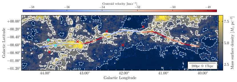
The ISM has a hierarchical structure and facilitates the formation of filaments that are governed by the Galactic potential on a large scale. Soler et al. (2020) present a network of H i filaments already evident in the diffuse atomic phase of the ISM that is structured mostly parallel to the Galactic plane. Only in a few cases is the orientation of the filaments locally no longer dictated by the overall drag of the Galactic disk but rather is determined by the effects of stellar feedback and strong magnetic fields. Soler et al. (2020) identify a unique H i filament that they have named “Maggie”, after the largest river in Colombia, the Río Magdalena. Maggie is shown to be a highly elongated filamentary cloud (see Fig. 1) extending over 4∘ on the sky in Galactic longitude. Given its central velocity of and assuming circular motion, Maggie is located approximately away from us and has a length of more than .
In this paper, we present a detailed study of the Maggie filament and aim to understand its physical nature. Is Maggie the precursor of large-scale molecular filaments? Are the physical and kinematic properties of filamentary molecular clouds inherited from an atomic counterpart in the diffuse ISM? Giant molecular filaments are to date the largest coherent entities identified in the Milky Way and have been subject of many recent studies investigating the evolution of large filaments with respect to the global dynamics of the Milky Way on the one hand and local stellar feedback on the other hand (Jackson et al. 2010; Ragan et al. 2014; Goodman et al. 2014; Wang et al. 2015, 2016; Abreu-Vicente et al. 2016; Zucker et al. 2015, 2018; Wang et al. 2020b).
The highly filamentary infrared dark cloud (IRDC) “Nessie”, first identified in Jackson et al. (2010), is argued to be one of the first in a class of filaments whose morphology is likely governed by the structural dynamics of the Galaxy. Goodman et al. (2014) dubbed this type of filaments “bones” of the Milky Way – highly filamentary molecular clouds whose formation, evolution, and shape could be closely linked to the global spiral structure of the Galaxy.
Zucker et al. (2018) utilized a standardized approach to re-analyze a set of Galactic filaments identified in the literature. In doing that, it is possible to draw meaningful conclusions and reliably compare physical properties between filaments rather than being subject to the systematics of selection criteria and different methodology. They found in their sample of filaments that the giant molecular filaments (GMFs), first identified in Ragan et al. (2014) and Abreu-Vicente et al. (2016), have the highest masses (10) while exhibiting the lowest column densities and star-forming activity, making them good candidates to be the immediate descendants of atomic ISM structures.
The GMFs are first identified as near and mid-infrared extinction features with a spatial extent of 100. Ragan et al. (2014) and Abreu-Vicente et al. (2016) then confirm velocity contiguity of the filaments via emission. Giant molecular filaments are not only associated with spiral arms but are also located in inter-arm regions.
The recently discovered Radcliffe wave (Alves et al. 2020) is a coherent 2.7 kpc long association of local molecular cloud complexes. It appears to be undulating above and below the Galactic midplane, and its three-dimensional shape (in position-position-position space) is well described by a damped sinusoidal wave. The Radcliffe wave provides a framework for future studies of molecular cloud formation and evolution with respect to the Galactic dynamics of the Milky Way.
Simulations find that giant molecular clouds often form as large filaments, and their formation can be related to the dynamics of the galaxy and position with respect to the spiral arm potentials. Smith et al. (2014a) use simulations of a four-armed spiral galaxy to investigate the formation of molecular gas structures. They find that high-density filaments tend to form in spiral arms while lower-density gas resides in long inter-arm spurs that are stretched by galactic shear. While the simulations account for the chemical evolution of the gas, they do not include the effects of self-gravity of the gas or stellar feedback.
Including both stellar feedback and self-gravity, smoothed particle hydrodynamics simulations of a high-resolution section of a spiral galaxy indicate that galactic shear between spiral arms plays a critical role in the formation of highly filamentary structures (Dobbs 2015; Duarte-Cabral & Dobbs 2016). Duarte-Cabral & Dobbs (2017) expand this analysis to the time evolution of these filaments, finding that giant molecular clouds tend to sustain their large filamentary shape before entering the spiral arms, where they are prone to being disrupted by local events of star formation and stellar feedback.
The CloudFactory simulations presented in Smith et al. (2020) strongly suggest that spiral arms and differential rotation tend to arrange molecular clouds in long filaments that are likely to fragment while regions of clustered feedback randomizes the orientation of them. Molecular filaments that are dominated by galactic-scale forces also exhibit low internal velocity gradients and are tightly confined to the galactic plane. Filaments formed in regions of higher turbulence due to supernova (SN) feedback show a range of orientations with respect to the galactic plane and are more widely distributed.
The systematic search for atomic counterparts to molecular clouds poses a challenging task. By means of the 21cm-line of H i emission it is generally possible to probe large atomic clouds in the ISM but it has proven difficult to identify them as clearly defined objects in the inner Galactic plane. Traditionally, H i clouds are then either observed at high Galactic latitudes (e.g. Kalberla et al. 2016) or they must have velocities significantly different than those imposed by the Galactic rotation (e.g. Wakker & van Woerden 1997; Westmeier 2018).
As the analysis of H i emission in the Galactic plane within the solar circle suffers from the kinematic distance ambiguity, any H i cloud with (in the first Galactic quadrant) might be the product of blending foreground and background components that correspond to the same line-of-sight velocity. However, at negative velocities any H i structure can be identified with less line-of-sight confusion111vice versa in the fourth Galactic quadrant. (see e.g. Brand & Blitz 1993).
Additionally, the physical properties of atomic hydrogen are not straightforward to derive from emission studies alone. In thermal pressure equilibrium, theoretical considerations based on ISM heating and cooling processes predict two stable phases of atomic hydrogen at the observed pressures in the ISM, namely the cold neutral medium (CNM) and warm neutral medium (WNM; Field et al. 1969; McKee & Ostriker 1977; Wolfire et al. 2003; Bialy & Sternberg 2019). Observations of H i emission are thus generally attributed to both CNM and WNM, which have significantly different physical properties. The CNM is observed to have temperatures and number densities of while the thermally stable WNM exceeds temperatures of 5000 with number densities (Heiles & Troland 2003; Kalberla & Kerp 2009). For densities between and , the gas is thermally unstable (denoted by UNM: unstable neutral medium) and it will move toward a stable CNM or WNM branch under isobaric density perturbations (Field 1965).
Throughout the scope of this paper, we use the analytic model presented in Wolfire et al. (2003) as a standard reference. According to this, the two stable atomic hydrogen phases can coexist in thermal equilibrium over a narrow range of pressures, , that is governed by the total heating and cooling rates of the interstellar gas (see e.g. the phase diagrams shown in Fig. 7 in Wolfire et al. 2003). The dominant heating process under typical ISM conditions is photoelectric (PE) heating from dust grains and polycyclic aromatic hydrocarbons (PAHs). The WNM is mainly cooled by Ly emission while the most efficient cooling mechanism of the CNM is metal-line fine-structure emission primarily excited by collisions with electrons and neutral hydrogen atoms. Assuming a constant ratio of the cosmic-ray (or X-ray) ionization rate, , to the intensity of the UV interstellar radiation field, , PE heating is proportional to . If is then increased (decreased), the density at which metal-line cooling balances heating must increase (decrease) in the same manner. As a result, the pressure range at which both WNM and CNM occur shifts to higher or lower values in proportion to .
Furthermore, the metallicity and dust abundance are crucial parameters for the thermal balance. If the metallicity is moderately lowered, the equilibrium pressure range dictating the WNM and CNM properties decreases since the dust-to-gas ratio and associated PE heating rate decreases more rapidly with decreasing than does the metal-line cooling222Here we do not consider the effect of cosmic ray heating that becomes the dominant heating mechanism at metallicities (see Fig. 2 in Bialy & Sternberg 2019). (Bialy & Sternberg 2019, see their Fig. 4).
In an attempt to observationally isolate the CNM from the bistable emission, H i self-absorption (HISA; Gibson et al. 2000; Li & Goldsmith 2003; Wang et al. 2020c; Syed et al. 2020) is a viable method to study H i clouds in the inner Milky Way but it heavily depends on the presence of sufficient background emission.
The Maggie filament was discovered in Soler et al. (2020) via H i emission in The H i/OH Recombination line survey of the inner Milky Way (THOR; Beuther et al. 2016; Wang et al. 2020a). It is identified as a large coherent filament using a Hessian matrix approach. This method allows to systematically identify filamentary structures by their spatial curvature that emerge as second derivative signatures in the H i emission maps of the THOR survey.
We follow up on this discovery and derive the physical properties of the Maggie filament in the subsequent analysis. This paper is organized as follows. We introduce the observations and data in Sect. 2 and outline the method we use for the spectral decomposition of the H i emission. We present the fundamental properties of Maggie and show the results of the kinematics and column density in Sect. 3. In Sect. 4 we examine Maggie for molecular counterparts and explore the possible formation process of Maggie. We also discuss the implications of the velocity and column density structure. Finally, we review the relationship between Maggie and giant molecular filaments and draw our conclusions in Sect. 5.
2 Observation and methods
2.1 HI 21 cm line and continuum
In the following analysis we employ the H i and 1.4 GHz continuum data from the THOR survey. A complete overview of the THOR survey and the data products is given in Beuther et al. (2016) and Wang et al. (2020a). We investigate the kinematics based on the H i emission data, where the 1.4 GHz continuum emission has been subtracted from the THOR H i observation during data reduction. The final H i emission data (THOR-H i) have been obtained from observations with the Very Large Array (VLA) in C- and D-configuration, as well as single dish observations from the Greenbank Telescope. The data have an angular resolution of and the noise in emission-free channels is 4 at the spectral resolution of . The covered velocities range from to .
In Sect. 3.3 we correct for the optical depth that we measured against discrete continuum sources. We therefore select the THOR H i+continuum data that consist of VLA C-array configuration data only (THOR-only). THOR-only data have a higher angular resolution of 14″, making them suitable to study absorption against discrete continuum sources. Since this data set consists of interferometric observations only, large-scale H i emission is effectively filtered out. This large-scale filtering due to the interferometer can be exploited when only discrete continuum sources are of interest.
2.2 Gaussian decomposition
The THOR H i emission spectra show Gaussian-like structures at negative velocities, with usually three or fewer components superposed. We therefore use the fully automated Gaussian decomposition algorithm GaussPy+333https://github.com/mriener/gausspyplus (Riener et al. 2019) to study the kinematics of the filament.
GaussPy+ is a multi-component Gaussian decomposition tool based on the earlier GaussPy algorithm (Lindner et al. 2015) and provides an improved fitting routine and a fully automated means to decompose emission spectra using machine-learning algorithms. GaussPy+ automatically determines initial guesses for Gaussian fit components using derivative spectroscopy. To decompose the spectra, the spectra require smoothing to remove noise peaks while retaining real signal. The optimal smoothing parameters are found by employing a machine-learning algorithm that is trained on a subsection of the data set.
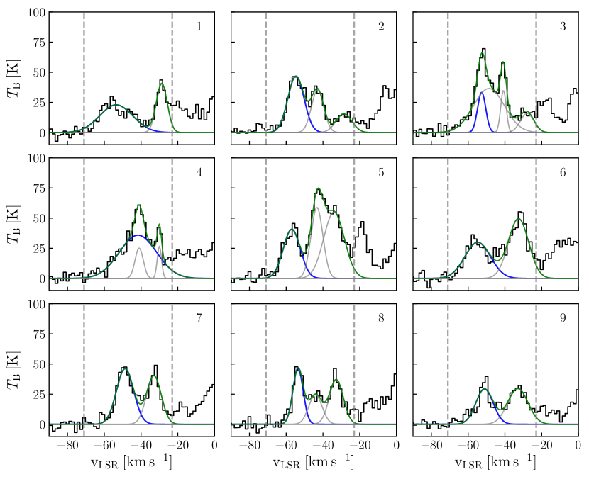
As Maggie is found at negative velocities and the H i emission toward the inner Galactic plane with is ubiquitous in the spectra, it would not be sensible to fit the whole spectra with GaussPy+. Instead, to save computational resources and achieve a better decomposition performance, we masked all spectral channels at velocities and (see Fig. 2). Maggie has velocities around (see Fig. 3 and Sect. 3.2) and we aim to disentangle components that might blend in with Maggie.
However, it is essential to reliably estimate the noise in the spectra to obtain good fit results. GaussPy+ comes with an automated noise estimation routine as a preparatory step for the decomposition. For this step, we supplied the full spectra to GaussPy+ as the masked spectra might not contain enough noise channels. The noise map derived in that way was then used for the decomposition of Maggie.
We ran the GaussPy+ training step with 500 randomly-selected spectra from the H i data to find the optimal smoothing parameters for the fitting, as recommended in Riener et al. (2019). For H i observations, we would expect both narrow and broad line widths owing to the multiphase (i.e. WNM-CNM-UNM) nature of H i emission. To account for that, we chose not to refit broad or blended components, parameters that can easily be adjusted in the GaussPy+ routine.
After the initial fitting, the algorithm applies a two-phase spatial coherence check that can optimize the fit by refitting the components based on the fit results of neighboring pixels. Figure 2 shows example spectra along the Maggie filament marked in Fig. 3, and the final fit results from the GaussPy+ decomposition. Between two and three components were typically fitted by GaussPy+ in the given velocity range. In every pixel spectrum, we selected the component with the lowest centroid velocity as the “Maggie” component (see Sect. 3.2) since no significant portion of H i emission is found at . Due to blended components and strong emission at higher velocities, a selection based on amplitude of the components fails to recover the structure identified in Soler et al. (2020) as the Maggie filament.
3 Results
3.1 Location, distance, and morphology
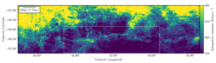
Figure 1 shows the integrated H i emission covering the Galactic plane at longitudes and latitudes and , respectively. The filament Maggie subtends an area from to in Galactic longitude and latitude, and has a velocity around with respect to the local standard of rest (). In this region in position-position-velocity (--) space, the Galactic H i disk shows a warp toward higher latitudes (see e.g., Burton 1988; Dickey & Lockman 1990; Sparke 1993; Dickey et al. 2009), which places Maggie at a location significantly displaced from the Galactic midplane. The H i midplane lies even beyond the coverage of the THOR survey at . Therefore, the midplane and Maggie are separated by at least on the plane of the sky.
In the forthcoming analysis we assumed the Galactic rotation model by Reid et al. (2019) and used the Bayesian distance calculator of the BeSSeL survey (Reid et al. 2016) to translate the location in -- space into a physical distance. Maggie’s estimated distance away from us is and its distance to the Galactic center is . This physical scale locates the filament below the Galactic midplane, which is greater than the average H i scale height (200) at this Galactocentric radius (Kalberla & Kerp 2009).
The Maggie filament discloses a hub-like feature in the east, on which smaller-scale filaments appear to converge, and a tail that thins out toward the west. The northwestern part shows a connection to the midplane, potentially feeding off the H i material located at higher latitudes. Most of the filament, however, appears to be disconnected from the Galactic midplane material.
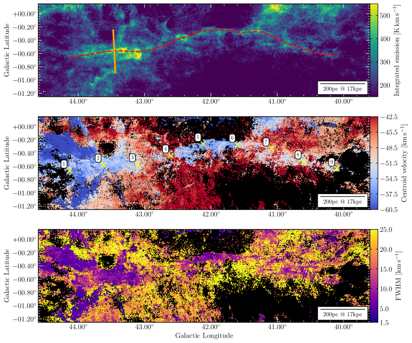
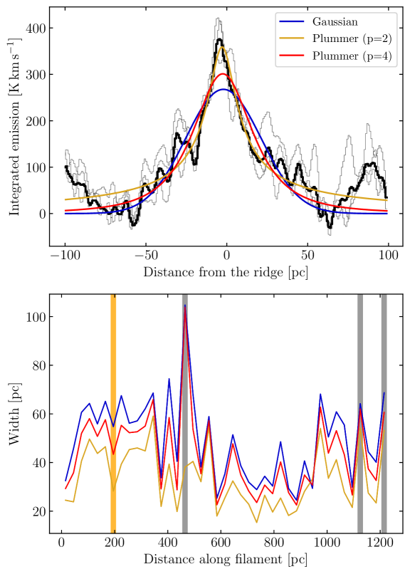
We define a backbone that runs through Maggie by selecting a spline based on visual inspection of the integrated emission (see top panel in Fig. 3). The length and width of Maggie are estimated using the Filament Characterization Package444https://github.com/astrosuri/filchap (FilChaP; Suri et al. 2019). These properties are not heavily affected by a potential misplacement of Maggie’s spine.
The length of the filament as marked by the red spine in the top panel of Fig. 3 is assuming a distance of . The uncertainty in length is dominated by the uncertainty in distance. The width of the filament was estimated using the integrated emission map shown in Fig. 3. We took perpendicular slices of width with a step size of (3beam) along the filament. We then averaged the radial emission profiles over three neighboring slices and fitted Gaussian and Plummer-like functions to the averaged emission profile. Plummer-like functions (as functions of cylindrical radius ) have the form
| (1) |
where is the power-law index, is the density at the center of the filament, and is the characteristic radius of the flat inner portion of the density profile. More details about the fitting can be found in Suri et al. (2019).
Plummer-like functions are used to describe the radial column density (i.e. integrated emission in the optically thin limit) profile of a cylindrically shaped filament that has a flat density distribution up to and a power-law fall-off beyond (Arzoumanian et al. 2011). We used constant power-law indices and 4 for the Plummer-like functions due to the degeneracy between and (and therefore ) in finding the best fit solution (see Smith et al. 2014b). The power law index describes the Ostriker (1964) model of an isothermal filament in hydrostatic equilibrium. The power-law index is derived by Arzoumanian et al. (2011) as a free fit parameter from small-scale filamentary structures seen in Herschel data and might be attributed to non-isothermal or magnetized filaments (see Arzoumanian et al. 2011, and references therein).
The fitted widths along the filament are shown in Fig. 4, with zero distance at the outermost point in the east. The widths derived from Gaussian fits are systematically larger than the widths estimated by Plummer-like functions. While the Plummer-like function with an index of is able to reliably reproduce individual peaks (upper panel of Fig. 4), the fits on average underestimate the width of the emission profiles. Gaussian fits do not fully recover the amplitude of the profiles but give a more accurate representation of the wings. As the noise and blending of different emission features make it difficult to determine which function represents the emission profiles best, we consider the fits equally good. The reduced chi-squared distributions of the fits are similar and do not allow any preference of a fitting function. Three positions along the filament (vertical gray bars in Fig. 4) are discarded as the fits gave no reliable results, regardless of the fitting function. For simplicity, we report the average width taken over the full length of the filament. Taking into account all fitting methods, the average width is , which is well resolved by the beam of the THOR observations corresponding to a spatial scale of . The uncertainty is dominated by the variance of the measured widths along the filament. The filament width is only weakly affected by the velocity integration range. If we integrate the emission over the velocity range –57.5 to –42.5, the average filament width becomes 44 pc, which is well within the uncertainty of our derived width. However, due to blending emission components toward higher velocities, the derivation of the filament width becomes increasingly difficult with increasing velocity integration range. We therefore constrain the integration range to roughly the lower and upper quartile of the velocity distribution (see Sect. 3.2).
One of the characteristics that is usually used to define filaments is the projected aspect ratio (see e.g., Zucker et al. 2015, 2018). Taking the average width, Maggie has an aspect ratio of (30:1). Although Maggie is identified through atomic line emission, as opposed to the selection of molecular filaments investigated by Zucker et al. (2018), Maggie roughly agrees with the overall aspect ratios of other large-scale filaments (Wang et al. 2015) and the identified Milky Way bones (Goodman et al. 2014; Zucker et al. 2015).
3.2 Kinematics
In the following section, we focus in detail on the kinematic properties of Maggie. We show in the middle and bottom panel of Fig. 3 the maps of the fitted centroid velocities and line widths of the first fit component (corresponding to the lowest-velocity component of the GaussPy+ decomposition), to which we refer as the “Maggie component” in the following. Accordingly, the second fit component refers to the next component at higher centroid velocity. Overall, the peak velocities along the filament vary between and and exhibit an undulating pattern (see also Fig. 9). For the most part, the velocity map clearly reflects the spine of the filament, as components off the spine have significantly larger velocities but are picked up as the first component in the absence of Maggie. Given the large spatial scales, the velocities along the spine show a smooth gradient of less than , a kinematic property that satisfies the bone criteria in Zucker et al. (2015).
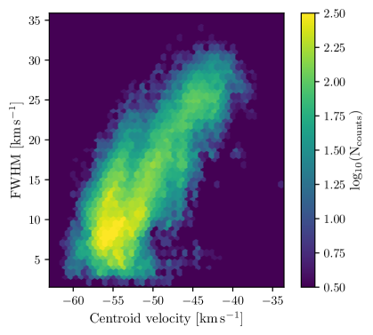
The line widths as well as centroid velocities shown in Fig. 3 indicate a stark contrast between the filament and the background. Furthermore, the kinematics in terms of the centroid velocity and line width along the filament spine are moderately correlated, where narrow line width corresponds to lower centroid velocity. Figure 5 presents the relationship between the centroid velocity and line width along the 40 pc-wide spine of the filament. The Pearson correlation coefficient between the velocity and line width distribution is 0.76, implying that under the assumption of a linear dependence 60% of the variance in the line width distribution can be explained by the scatter present in the centroid velocity distribution. We note that this does not necessarily imply a causal relation between the line width and velocity. Rather, this correlation is likely to be due to contamination from background gas at positions where the filament emission is less well defined and difficult to disentangle from blending components.
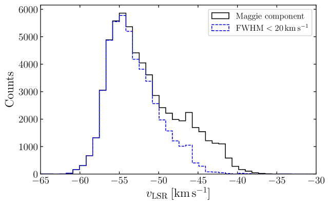
Figure 6 shows the histogram of centroid velocities of Maggie, where all individual pixel positions along the -wide spine of the filament are being sampled. The centroid velocities along the filament exhibit a strong peak at , with some skewness toward that might be attributed to velocity blending of broad WNM components at higher velocities.
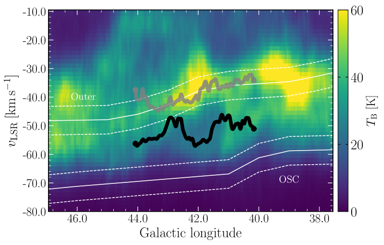
Figure 7 offers a position-velocity view of Maggie and its location with respect to the average H i emission. We also overplot the predicted locations of the spiral arms as given by Reid et al. (2019). The bulk of H i material and the second fit component of our spectral decomposition trace out the spine of the Outer arm remarkably well while Maggie exhibits an offset of 5–15. Given the distance from the midplane, neither spatially nor kinematically can Maggie be associated with any spiral arm structure. We note, however, that different spiral arm models can vary by or more in position-velocity space, a concern raised by Zucker et al. (2015) when classifying bones of the Milky Way.
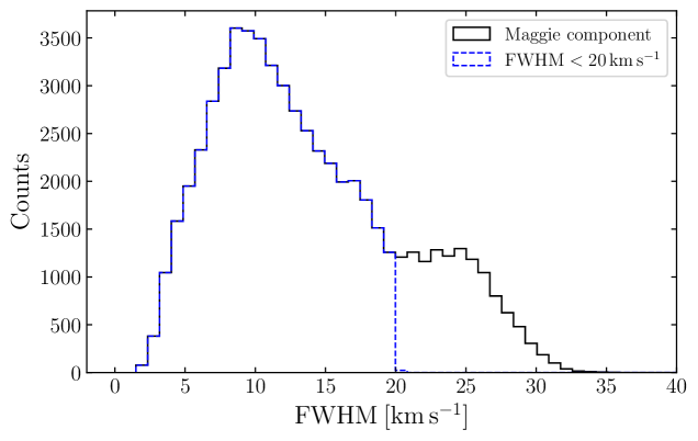
The histogram of line widths in Fig. 8 shows a broad distribution, with line widths between and . The histogram has a peak around and a shoulder that extends to . We additionally show in Figs. 6 and 8 the histograms corresponding to velocity components with a line width , discarding the shoulder in the line width distribution. The median values of the total centroid velocity distribution is , and only taking into account line widths , the median shifts to .
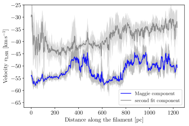
To study the kinematic structure with respect to the position along the filament we show in Fig. 9 the average velocity of each -wide slice weighted by the amplitude at each pixel position. The uncertainties are estimated by the standard deviation of each slice. The wave-like velocity structure of Maggie is now more clearly visible. The Maggie velocities beyond around distance (corresponding to the region around spectrum 4 in Fig. 2) are difficult to clearly separate from the second fit component. We note that the mean velocity and particularly line width have to be treated with some caution as the velocity blending makes it difficult to distinctively identify Maggie in this part of the region. We revisit the velocity structure in Sect. 4.2.2 to investigate signatures of characteristic spatial scales.
3.3 Column density and mass
Measuring H i absorption against strong continuum sources allows us a direct derivation of the optical depth. We therefore use the high angular resolution H i+continuum data, that consist of VLA C-array observations only, to filter out large-scale emission and measure H i absorption against discrete continuum sources. We measured HI+continuum spectra against seven continuum sources taken from Wang et al. (2018) that have brightness temperatures for a sufficient signal-to-noise ratio. The sources are located both within and outside the area of Maggie (i.e. within and outside the contour at , see later in this section). Since the synthesized beam of the native C-configuration data is 14′′, we extracted an average H i+continuum spectrum from a ( pixels) area. To the first order, we can then estimate the H i optical depth by (see Bihr et al. 2015)
| (2) |
where is the H i brightness temperature against the continuum source and is the brightness of the continuum source. Using the optical depth, we compute the H i spin temperature with
| (3) |
We measured the H i brightness at an offset position using the combined THOR H i data (see Sect. 2.1). We therefore selected an annulus around each source with inner and outer radii of 60″and 120″, respectively, to measure an averaged .
All spectra measured against Galactic H ii regions do not exhibit any absorption features in the velocity range of Maggie (Tab. 5). This gives additional support to the argument that the Maggie filament is in fact on the far side of the Galaxy as Galactic H ii regions are located in the foreground and can therefore not be detected in absorption. Furthermore, we find that no absorption is evident in the spectra of both Galactic and extragalactic continuum sources offset from the line of sight of Maggie.
| Source ID | Glon [∘] | Glat [∘] | [K] | Type | L.o.s. | Absorption |
|---|---|---|---|---|---|---|
| G43.921-0.479 | 43.92 | -0.48 | 304 | extragal. | ✓ | ✓ |
| G43.890-0.783 | 43.89 | -0.78 | 481 | H ii | ✗ | ✗ |
| G43.738-0.620 | 43.74 | -0.62 | 503 | extragal. | ✓ | ✓ |
| G43.177-0.519 | 43.18 | -0.52 | 296 | H ii | ✓ | ✗ |
| G42.434-0.260 | 42.43 | -0.26 | 277 | H ii | ✗ | ✗ |
| G42.028-0.605 | 42.03 | -0.60 | 519 | extragal. | ✗ | ✗ |
| G41.513-0.141 | 41.51 | -0.14 | 205 | H ii | ✗ | ✗ |
The extragalactic continuum sources G43.738-0.620 and G43.921-0.479666The optical depth measurement against G43.921-0.479 is close to the detection limit and will not be discussed further here. However, the mean optical depth and velocity-integrated optical depth are consistent with the other source G43.738-0.620. are the only sources along Maggie against which we detect H i in absorption. We show in Fig. 10 an overview of the optical depth and spin temperature measurement toward G43.738-0.620.
The top panel illustrates the averaged H i emission profile. In pressure equilibrium, the two stable phases of atomic hydrogen (CNM and WNM) both contribute to the emission. It is difficult to disentangle the properties of either phase from the emission alone, so the information from the absorption profile is critical to learn about the nature of the atomic gas. As the optical depth is proportional to , we assume that any absorption measured toward the continuum is due to the CNM.
For simplicity we fit both the emission and absorption profile in this specific case (Fig. 10) with a single Gaussian component. The line width of the emission profile is and therefore significantly wider than the absorption line (), suggesting that there is contribution to the emission from a broader component that is not evident in the absorption spectrum. However, the line width contributions are not able to pin down the column density fractions of either the CNM or WNM as the (kinetic) gas temperatures are unknown and the line widths can be significantly broadened by non-thermal effects. The total line width, however, can therefore set an upper limit on the kinetic temperature (Heiles & Troland 2003). We note that the non-thermal contribution to the CNM component, due to effects such as turbulent motion, should be dominant as the thermal line width of the CNM even with the loose constraint (e.g. Heiles 2001; Heiles & Troland 2003) would account for a line width .
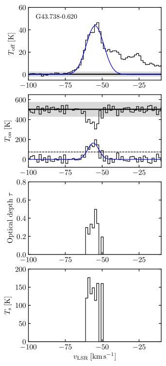
The optical depth above the limit, that we ascribe to the CNM, is plotted in the third panel of Fig. 10. The mean and velocity-integrated optical depth over the velocity range of Maggie is and , respectively. We note that the reported values in Wang et al. (2020a) are inferred from integrating over the whole velocity range of the THOR survey and are thus significantly larger. We use the optical depth and brightness temperature from the emission profile to compute the spin temperature (Eq. (3)) in the bottom panel of Fig. 10. The mean spin temperature is . Owing to the mixing of warm and cold HI along the line of sight, this spin temperature should not be interpreted as a gas kinetic temperature. Rather, it is a density-weighted harmonic mean of the kinetic temperature under the assumption that (see Dickey et al. 2000, 2003, 2009). If we assume that the warm HI does not contribute significantly to the optical depth, that the correction for HI self-absorption is negligible and that the CNM has a roughly constant temperature, then we can derive the CNM fraction via
| (4) |
where and are the column density of the CNM and WNM, respectively, and is the CNM spin temperature. A representative value for the CNM spin temperature should lie within (Heiles & Troland 2003; Strasser & Taylor 2004; Dickey et al. 2009), which is also in good agreement with the theoretical models by Wolfire et al. (2003) at the Galactocentric distance . This conservative estimate gives a CNM fraction in the range . Applying this finding to the whole cloud, Maggie should consequently be composed of a significant fraction of CNM.
We estimate the column density of the atomic hydrogen using (e.g. Wilson et al. 2013)
| (5) |
where is the total column density of H i in units of as a function of the H i spin temperature and optical depth integrated over the velocity . The spin temperature is , where is the brightness temperature of the H i emission. The optical depth correction of the column density scales as , resulting in a correction factor of for . We integrated the column density from to , taking into account the predominant velocities of Maggie. The column density then has values in the range . We used the observed THOR-H i emission data instead of the individual Maggie component of the decomposition to compute the column density although there might be additional contributions from components blending in at a similar velocity. We show in Appendix A that the integrated Maggie component is not spatially coherent in amplitude and shows patches of lower amplitude, likely owing to the existence of blended components that are difficult for GaussPy+ to disentangle. To estimate a maximum fraction of unrelated blended emission contributing to the column density, we compare the two column density maps. We find that the column density (and ultimately mass) inferred from the single Maggie component (App. A) is smaller by approximately 30%.
We note that choosing a single fit component as the “filament” can be problematic as the multiphase nature of H i emission may have multiple components at similar velocities contributing to Maggie. Here, we define Maggie by the centroid velocity of a single component and do not impose any restrictions on the H i phase of Maggie, which is reasonable in order to study the velocity structure. Yet, by choosing a single component we might include only one H i phase. GaussPy+ does not explicitly check for spatial coherence in amplitude or line width but for coherence in number of components and their centroid velocity. As we argue above, in a CNM-WNM mixture of the gas it is then difficult to characterize Maggie based on the centroid velocity of a single component alone. One way to fit and identify multiple phases in H i emission spectra, is to introduce spatial regularization terms to the loss function of the fitting that are able to cluster different phases (here: CNM and WNM) even if close in velocity (Marchal et al. 2019). This approach, however, is computationally expensive and will not be followed here.
The picture of a well-defined CNM phase layer within a WNM envelope assuming thermal pressure equilibrium might be overly simplified. Instead, we would expect a clumpy CNM embedded in a ‘sea’ of WNM, implying that the CNM has a lower volume and area filling factor than the WNM and a strong density contrast (Kalberla & Kerp 2009). The patchy structure seen in Fig. 15 could be a reflection of the clumpy structure of the CNM. Lower intensity in small-scale structures could also hint at CNM that has already converted to molecular gas (see Sect. 4.4). If we want to infer the global multiphase column density of Maggie, however, it is beneficial to examine the properties of the filament by means of the integrated emission rather than using a single GaussPy+ fit component, in order to avoid missing mass.
Figure 11 shows the mass surface density map of Maggie derived from the observed emission data. The mass surface density reaches values of more than 8.0777We relate the total hydrogen column density to the visual extinction using (Güver & Özel 2009). We take into account the molecular column density using the upper limit estimated in Sect. 4.1. toward the eastern hub and its distribution is constrained to within one order of magnitude (see Sect. 4.3). Wolfire et al. (2003) predict an average midplane thermal pressure at the Galactocentric radius of . We can estimate the expected length scale of Maggie along the line of sight by , where we set the kinetic temperature to be close to the density-weighted mean spin temperature . Since Maggie is significantly below the midplane, the pressure is likely to be smaller than . Thus, we assume a canonical pressure of . At the mean column density of (see also Sect. 4.3), the line-of-sight length is estimated to be 22, which is roughly consistent with the on-sky width of 40 pc given the uncertainty in temperature and pressure.
Because of the diffuse nature of the WNM that is significantly contributing to the observed H i emission it is difficult to define a clear edge of the filament. We therefore estimate two different masses: a “diffuse mass” in which the dense filament is embedded (mass above ), and a “dense filament mass” which resides within an approximately closed contour at the level () that roughly corresponds to the filament width obtained in Sect. 3.1.
The total diffuse mass including the dense filament is . As mentioned above, due to its diffuse nature the mass derivation of the H i has a high uncertainty as it is dependent on the selection of filament regions taken into account. Varying the contour level by to estimate the uncertainty, the dense filament mass is . The atomic mass of Maggie therefore is comparable to the highest masses of large-scale filaments identified in the Milky Way (Ragan et al. 2014; Abreu-Vicente et al. 2016; Wang et al. 2015, 2016; Zucker et al. 2015, 2018), providing a large atomic gas reservoir to potentially host molecular cloud formation.
If we take the column density we use to define the edge of the “dense” filament and assume that the width of the filament is the same along the line of sight as in the plane of the sky, we obtain a density of , which equates to an H nucleus number density of roughly . This is intermediate between the average densities we expect for the WNM and CNM at this Galactocentric radius (Wolfire et al. 2003), which is best explained by the filament being a mix of both components.
However, given a mean density of , we point out that either the CNM mass fraction must be higher or that a substantial fraction of the WNM must be in an unstable phase to be in agreement with the theoretical model given in Wolfire et al. (2003). This follows from the mass conservation:
| (6) |
where is the volume filling fraction of the CNM, is the CNM number density, and is the ratio of the CNM and WNM temperature in pressure equilibrium. The CNM mass fraction can then be expressed as
| (7) |
Assuming the Wolfire et al. (2003) CNM-WNM model, with the CNM mass fraction is higher than our assumed values. For example, even for a CNM density (the maximum CNM density at ; Wolfire et al. 2003), the CNM fraction is still . The mean density can be brought into agreement with the previously derived CNM fraction of 0.5 if the temperature ratio becomes , which corresponds to a mean temperature in the unstable regime 1000–2000, compared to the higher temperatures of the classical WNM around 6000 K. Observational works have found the fraction of H i in the unstable phase to be at least 20–50% (Heiles & Troland 2003; Roy et al. 2013b; Murray et al. 2015, 2018; Nguyen et al. 2019), possibly even higher (Koley & Roy 2019).
4 Discussion
4.1 Molecular gas tracers, continuum, and dust
What is the molecular gas fraction of Maggie and are there signatures of molecular cloud formation? To address this, we investigated the molecular lines , , and O (–0) using the Milky Way Imaging Scroll Painting (MWISP; Su et al. 2019) survey. The rms noise of the data is for at the velocity resolution of and for and O at resolution. The spatial resolution in all three tracers is 50″.
In all three tracers, we detect no molecular gas emission in the velocity range between and . We show in Appendix B a map of the integrated emission as an example. To estimate the molecular hydrogen content, we used the CO- conversion factor (Dame et al. 2001). We determined an upper limit at for the molecular surface density of . Since the sensitivity limit is close to the observed H i column densities, we cannot entirely dismiss the presence of CO-bright gas.
Indeed, Nakanishi et al. (2020) identify molecular gas clumps toward Maggie within small-scale H i clouds that they infer from a dendrogram analysis of the VGPS H i data (Stil et al. 2006). The average size of the H i clouds is 5 pc. They derive the molecular mass by summing the brightness temperature of the FUGIN data (Umemoto et al. 2017) within each H i cloud, including voxels with a brightness temperature lower than the noise. In doing that, diffuse emission can be recovered in the same manner as stacking emission spectra. The total mass of all 353 identified cloudlets that are within the dense filament contour at (area filling factor 0.21) is 6, only a small fraction of the H i mass (0.08), with the cloudlets’ average surface density being 2.5 that is consistent with our upper limit. The mean molecular mass fraction of the H i clouds is 0.2 of the total gas mass (Nakanishi et al. 2020). Naturally, the H i “leaves” of the dendrogram analysis sample the highest-density parcels of the medium, hence a portion of the total molecular mass outside the H i clouds might be missed.
In addition, CO might not always be a good tracer of molecular hydrogen as “CO-dark” could account for a significant fraction of the total (Pineda et al. 2008; Goodman et al. 2009; Tang et al. 2016), particularly at low column densities (Goldsmith et al. 2008; Planck Collaboration et al. 2011). The CO-dark fraction has furthermore been observed to increase with Galactocentric distance (Pineda et al. 2013). Simulations of molecular gas in Milky Way type galaxies indicate that the CO-dark fraction is indeed higher in regions of lower surface density (Smith et al. 2014a). CO observations at visual extinctions could underestimate the molecular hydrogen content by a significant fraction (Glover & Mac Low 2011).
As OH may be a better molecular gas tracer than CO in atomic-molecular transition regions at low column densities (e.g. Tang et al. 2017), we inspected the strongest OH line at in the THOR OH data (see Rugel et al. 2018). The THOR OH data consist of VLA C-array observations only, so large-scale emission cannot be recovered due to the missing flux on short spacings. However, we can derive an OH abundance from OH absorption measurements against continuum sources. At the velocity range of Maggie, no absorption is found against any of the continuum sources listed in Tab. 5. We note that depending on the peak flux of the continuum source and opacity of the OH line, the detection limit could be above the expected OH column density. The presence of molecular gas traced by OH can therefore not be ruled out. Follow-up OH observations at higher sensitivity will address this in a future study.
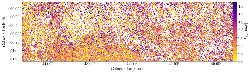
We investigated the possibility of Maggie being a foreground structure by examining the extinction of stars up to a distance of 5 kpc using the early installment of the third Gaia data release (Gaia Collaboration et al. 2021). The -band extinctions are obtained using the Rayleigh-Jeans Colour Excess (RJCE, Majewski et al. 2011) method which combines near- and mid- infrared data from the Two Micron All-Sky Survey (2MASS; Skrutskie et al. 2006) and the Wide-Field Infrared Survey Explorer (WISE; Wright et al. 2010), respectively. The Gaia Archive888https://gea.esac.esa.int/archive/. provides the crossmatch of Gaia sources with both the 2MASS and WISE catalogues.
In the presence of an obscuring medium, for example an atomic cloud, high extinction in the densest parts would prevent the detection of stars in the Gaia sample, yet extinction toward the outer portions of the cloud can still be detected in order to trace its silhouette. Figure 17 presents the obtained -band extinctions toward Maggie for sources up to a distance of 5 kpc from us. If Maggie were located within 5 kpc from the Sun, higher extinction stars would represent its shape in the - plane. However, since no signature of Maggie emerges from the extinction map, this indicates that Maggie is not a foreground cloud with large deviation from the Galactic rotation velocity.
We furthermore detect neither extinction features in the Spitzer Galactic Legacy Infrared Mid-Plane Survey Extraordinaire (GLIMPSE; Churchwell et al. 2009) that might hint at the presence of IRDCs nor any excess infrared emission or signatures of stellar activity as observed in all bands of GLIMPSE and the Improved Reprocessing of the IRAS Survey (IRIS; Miville-Deschênes & Lagache 2005). There are two possible reasons for not detecting IRDC features: 1) Maggie has not formed cold, dense molecular regions on a large scale such that there exist no IRDCs within Maggie or 2) Maggie is too distant to be observed as an IRDC due to the lack of emission background.
We have also examined the high-sensitivity maps of Planck at 353, 545, and 857 GHz emission (Planck Collaboration et al. 2014) and the higher angular resolution Herschel Hi-GAL data (Marsh et al. 2017) to further search for signatures of Maggie. We do not detect Maggie in any of the continuum bands while noting that we are most likely dominated by foreground emission in the Galactic plane.
After taking a variety of surveys into consideration, Maggie appears to show no signs of stellar activity as it is mostly atomic, while molecular gas has formed only in high-density clumps on the smallest spatial scales (Nakanishi et al. 2020).
4.2 Kinematic signatures
4.2.1 Mach number distribution
In the following, we adopt a stable two-phase CNM-WNM model to derive the turbulent Mach number distributions. We estimate the three-dimensional scale-dependent Mach number of the filament assuming isotropic turbulence with , where and are the turbulent one-dimensional velocity dispersion and sound speed, respectively. The turbulent line width is calculated by subtracting the thermal line width contribution from the observed line width as
| (8) |
where , and are the observed, and thermal velocity dispersion, respectively. Since we expect the observed line width to be a combination of both CNM and WNM, and do not know the turbulent contribution to the observed line width of either H i phase, we compute a single Mach number for the two-phase medium using a weighted mean of the thermal line width and sound speed. The thermal velocity dispersion can be decomposed into a CNM and WNM component as
| (9) |
where and refer to the thermal velocity dispersion of the CNM and WNM, respectively. The combined velocity dispersion and sound speed can then be computed using the weighted mean kinetic temperature
| (10) |
where and are the kinetic temperatures of the CNM and WNM, respectively.
We assume that the kinetic temperature of the CNM is close to the spin temperature and set . In pressure equilibrium, Wolfire et al. (2003) predict a range of WNM kinetic temperatures between 4100–. As the densities of the WNM are low, the gas can usually not be thermalized by collisional excitation only, such that . Through excitation by resonant Ly photon scattering, sufficient Ly radiation can allow . The WNM spin temperature has been observed to be as high as (Murray et al. 2014). We therefore assume a mean WNM kinetic temperature of .
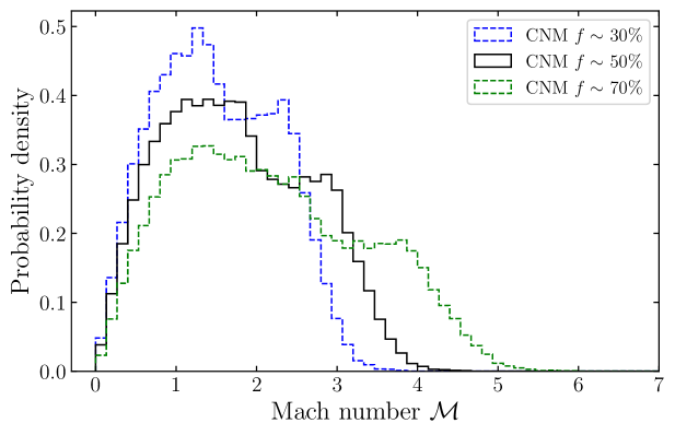
Since the thermal line width and sound speed scale as , the variation is moderate and does not change the Mach number significantly. We calculate three different Mach number distributions for , corresponding to .
Figure 12 shows the Mach number distributions of Maggie under different assumptions of the CNM fraction. The median Mach number is 1.5, 1.7, and 2.0 for the CNM fractions 30, 50, and 70%, respectively, which is generally in contrast to molecular filaments being driven by highly supersonic turbulence (e.g. Elmegreen & Scalo 2004). However, since we use a single mean kinetic temperature in each case, the Mach number distributions also reflect a slight bimodality that is already evident in the line width distribution (Fig. 8). While each Mach number distribution represents a different mixture of CNM-WNM gas, we note that the bump toward higher Mach numbers reflected in each distribution is due to the increased line widths associated with higher velocities, likely contaminated by blending background gas (see Sect. 3.2).
Numerical studies show that the condensation process toward a stable CNM phase depends on the properties of turbulence in the WNM (Seifried et al. 2011; Saury et al. 2014; Bellomi et al. 2020). These studies suggest that highly supersonic turbulence that is driven by compressive modes regulates the formation of a stable CNM phase as turbulent compression and decompression of the gas will be much more rapid than the cooling timescale. Once the gas has moved toward an unstable phase, that is the cooling timescale is shorter than the dynamical time , the gas can cool down fast enough to reach a stable branch of the CNM before being decompressed again (Hennebelle & Pérault 1999). On the other hand, a too low degree of turbulence cannot produce sufficient density fluctuations to sustain the formation of a thermally stable CNM. The WNM is mostly found in a sub-/transonic regime (e.g. Marchal & Miville-Deschênes 2020), therefore providing the dynamical conditions for thermal instability to grow efficiently to form a bistable H i phase.
Absorption studies show that a substantial fraction of H i in fact lies in a thermally unstable or transient phase (Heiles 2001; Heiles & Troland 2003; Roy et al. 2013a, b). Shifting the mean temperature of the WNM to an unstable regime around 1500 K leads to Mach numbers in the range .
4.2.2 Structure function
In order to investigate the velocity and column density structure of Maggie in a statistical sense, we compute the 1-D structure function (see Henshaw et al. 2020) of the data using
| (11) |
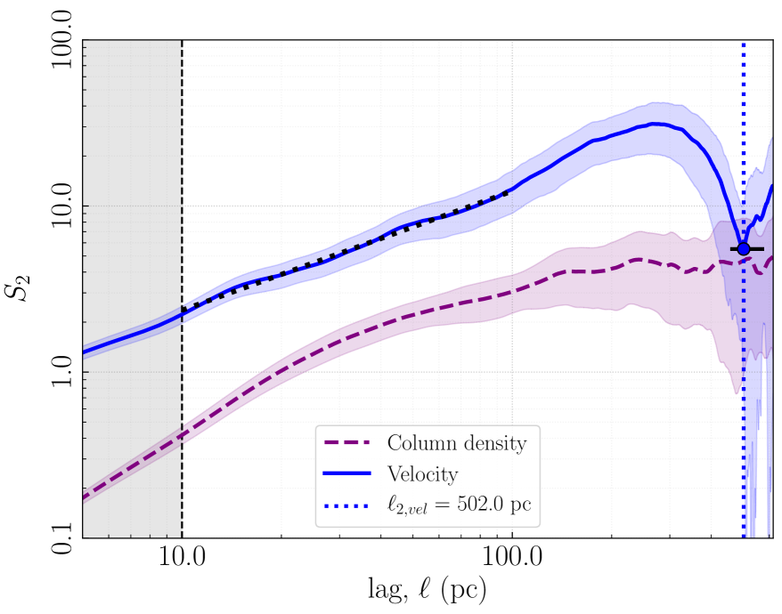
where is the absolute difference in the quantity measured between two locations and separated by . The brackets indicate the average of the quantity over all locations. The order of the structure function can be directly related to a physical quantity. We use the second order structure function, which in the case of the velocity structure is proportional to the kinetic energy of the line-of-sight component of the flow. We show in Fig. 13 the second order structure function derived from the weighted centroid velocity (Fig. 9), after having subtracted a 2-D plane fit to the velocity field in order to better examine the wave-like oscillation, and the column density along the -wide spine of Maggie. A significant local minimum is evident at the spatial scale of . Since the structure function is evaluated for pairs of positions that are separated by the lag , the maximum spatial scale at which the structure function can be fully sampled is given by half the total length of the filament. Therefore, the structure function is only computed over spatial scales . Consequently, the full velocity ‘dip’ cannot be recovered and we estimate the uncertainty of the scale by the difference between and , giving . This result confirms the wave-like pattern seen in Figs. 3 and 9.
The column density structure of Maggie does not show any characteristic length scale at which the structure function has a local minimum but roughly represents a power-law scaling, indicative of the scale-invariant behavior of a gas structure generated by turbulence (Elmegreen & Scalo 2004).
The phenomenological Kolmogorov relation for incompressible turbulence predicts a dissipationless cascade of energy in the inertial subrange, such that the kinetic energy transfer rate stays constant (Kolmogorov 1941). Due to the nature of the turbulent cascade, the velocity dispersion then increases with scale as , where , which we can relate to the power-law scaling of the second order structure function , where (see e.g. Elmegreen & Scalo 2004; Henshaw et al. 2020). We therefore fitted the velocity structure function with a power-law function of the form . We set the lower limit of the fitting range to three beam sizes (10 pc), below which no reliable structure functions can be recovered, and the upper limit at the approximate scale above which the structure function begins to turn over (100 pc). For Maggie we find in the case where we subtracted the 2-D plane fit, which is in good agreement with the expected power-law scaling in the sub-/transonic regime (see also Wolfire et al. 2003; Elmegreen & Scalo 2004; McKee & Ostriker 2007; Saury et al. 2014; Marchal & Miville-Deschênes 2020). While the dip in the velocity structure function is less pronounced if we do not subtract a 2-D plane fit, the power-law scaling remains the same with . These values are in agreement with the observational scaling exponents originally found by Larson (1979, 1981), who investigated the velocity dispersion–size relation in a sample of molecular clouds and clumps using different tracers. He utilized the radial velocity dispersion mainly in terms of the line width of optically thin lines, such that the relation between line width and individual cloud size can be interpreted as a correlation between velocity fluctuation and scale size (see also Scalo 1984). Larson (1979, 1981) found a velocity dispersion–size relation following a power law with an index , which is, although slightly larger, similar to the Kolmogorov relation. Systematic studies of more homogeneous samples of molecular clouds traced in CO found velocity scaling exponents in a range between 0.24 and 0.79 (see Table 2 in Izquierdo et al. (2021), which summarizes more than 40 years of observational work).
Izquierdo et al. (2021) find in their simulations that the scaling exponents lean toward lower values when molecular clouds are dominated by the influence of the Galactic potential rather than the effects of clustered SN feedback and self-gravity (see also Chira et al. 2019). This suggests that low velocity scaling exponents are associated with diffuse regions of low star forming activity (e.g. Federrath et al. 2010), which also favors the development of long filamentary structures (Smith et al. 2020).
Maggie’s velocity scaling is in better agreement with the lower end of the values found for molecular clouds (see above). This regime around 1/3 is indicative of Kolmogorov turbulence, and following Izquierdo et al. (2021), this turbulence may be caused by the Galactic potential rather than being driven by the effects of self-gravity or stellar feedback.
The existence of density enhancements that are spaced at a characteristic scale within a highly filamentary cloud would be in broad agreement with theoretical predictions of the fragmentation of a self-gravitating fluid cylinder due to the “sausage” instability (e.g. Chandrasekhar & Fermi 1953). As we find no characteristic scale in the column density structure, we argue that the effects of self-gravity have not yet become important and it is difficult to correlate the observed velocity signature with possible mechanisms driving the column density structure formation.
We caution, as pointed out in Sect. 3.3, that the column density is a product of both the CNM and WNM and is inferred from the integration over velocity. This could lead to a structure that smooths over an underlying higher-density CNM structure due to the diffuse nature of the WNM. The column density structure can furthermore not be described by single power-law alone. This could be due to the filament being a mix of both CNM and WNM and that the two phases have different turbulence scalings. With the WNM being more widespread, the structure function as probed by H i emission could be dominated by the warm diffuse gas on large scales while the CNM dominates the power-law on small scales (see e.g. Choudhuri & Roy 2019). The integrated emission might therefore not be the best estimator of the spatial distribution of the column density.
4.3 Column density PDF
What are the dominant physical processes acting within the cloud? To elaborate on the density structure of Maggie, we employ the commonly used probability density function (PDF) of the column density. The shape of column or volume density PDFs are used as a means to describe the underlying physical mechanisms of a cloud (e.g., Federrath & Klessen 2013; Kainulainen et al. 2014; Schneider et al. 2015). A log-normal shape of a PDF is considered a signature of turbulent motion dominating a cloud’s structure (see e.g. Klessen 2000). The magnitude of turbulence can furthermore be reflected in the width of a log-normal PDF and can then be associated with the Mach number (e.g., Padoan et al. 1997; Passot & Vázquez-Semadeni 1998; Kritsuk et al. 2007; Federrath et al. 2008; Konstandin et al. 2012; Molina et al. 2012), while noting that the turbulence driving scale and CNM-WNM mass ratio also affect the width of the PDF (Bialy et al. 2017b).
Molecular clouds that are subject to the increasing effect of self-gravity develop high-density regions, producing a power-law tail in their PDF (e.g. Girichidis et al. 2014; Burkhart et al. 2017). Many star-forming molecular clouds have been confirmed to show such power-law tails (Kainulainen et al. 2009; Schneider et al. 2013, 2016). Even before the effects of gravity become dominant, gravitationally unbound clumps can exhibit power-law tails due to pressure confinement from the surrounding medium (Kainulainen et al. 2011).
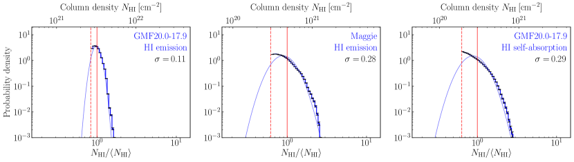
We show in Fig. 14 the normalized column density PDF (N-PDF) of Maggie taken above the limit at 3 (). The mean of the N-PDF is . The distribution varies within one order of magnitude and can be well described by a log-normal function of width . We caution that the shape and width of the resulting N-PDFs are sensitive to the region taken into account (Schneider et al. 2015; Lombardi et al. 2015; Ossenkopf-Okada et al. 2016; Körtgen et al. 2019). If we only consider column densities within an approximately last closed contour at 4, the N-PDF shows a narrower log-normal shape with a width smaller by .
Figure 14 presents a comparison between the N-PDF of Maggie and the optical depth corrected N-PDFs derived from H i emission and self-absorption toward the giant molecular filament GMF20.0-17.9 (Syed et al. 2020). The width of Maggie’s N-PDF comes close to the value found for the CNM gas traced by HISA and is larger than that of the atomic gas traced by H i emission toward the midplane (see also Wang et al. 2020c). However, the width of the CNM distribution is likely to be higher as the HISA N-PDF is limited by the column density range at which H i self-absorption can be detected.
Since we use the same data set and follow the same methodology for deriving the N-PDF as Wang et al. (2020c) and Syed et al. (2020), systematic differences should be minimized. Despite that, we note a slight cutoff in the PDF at . As we use a uniform optical depth correction for the whole cloud (Sect. 3.3), the optical depth could be underestimated in regions of high column density. If we assume a column density 10 and a FWHM line width 10, the peak optical depth becomes . The cutoff in the PDF could therefore be due to the cloud becoming optically thick and the width could then be underestimated.
Narrow log-normal shaped N-PDFs are commonly observed in the diffuse H i emission toward well-known molecular clouds (Burkhart et al. 2015; Imara & Burkhart 2016; Rebolledo et al. 2017). On the other hand, the HISA N-PDFs that trace the CNM show similar or somewhat broader distributions, indicative of the clumpy structure and higher degree of turbulence. The CNM-WNM mixture of Maggie, that is spatially more clearly defined than the material usually traced by H i emission, agrees with our previous findings and suggests that Maggie might be at the verge of becoming a dense filament forming out of the diffuse atomic ISM.
4.4 Molecular gas formation and timescale
Is Maggie expected to form molecular gas at its current evolutionary stage? We evaluate the surface density threshold of H i required to efficiently form molecular hydrogen, based on the analytical models by Sternberg et al. (2014), and Bialy & Sternberg (2016). These authors derive a steady-state H i-to- transition model assuming a slab irradiated isotropically on two sides by FUV flux. The expected H i surface density at the transition then is
| (12) |
(see Eq. (1) in Bialy et al. 2017a), where is the dust absorption cross section per hydrogen nucleus in the Lyman-Werner (LW) dissociation band (11.2–13.6) relative to the standard solar neighborhood value, is the ratio of the unshielded dissociation rate to formation rate, and is the average self-shielding factor in dusty clouds. The product is the formation-to-destruction rate ratio, accounting for shielding by line absorption and dust, and may be written as
| (13) |
(Sternberg et al. 2014; Bialy & Sternberg 2016), where is the free-space (unshielded) interstellar radiation intensity relative to the Draine (1978) field, and is the number density. The UV intensity exponentially decreases with Galactocentric distance (Wolfire et al. 2003). For , Wolfire et al. (2003) suggest . We note that this approximation is derived for the midplane and should be roughly constant up to the scale height of OB stars and could be significantly lower at larger distances from the plane. Since Maggie’s distance from the plane is an order of magnitude greater than the OB scale height in the solar neighborhood (Reed 2000), the UV intensity should be viewed as an upper limit with a relative uncertainty of at least 40% (see also Elias et al. 2006)
The dust absorption cross-section can be estimated as the inverse of the gas-to-dust ratio at the position of Maggie relative to the value in the local ISM if we assume that the dust grain properties are the same in the outer Galaxy. Giannetti et al. (2017) derive a gas-to-dust ratio as a function of galactocentric distance and metallicity based on C observations. Their reported gas-to-dust gradient predicts for Maggie and 141 as a local value for (Reid et al. 2019). The relative dust absorption cross-section then becomes . With the estimated number density of (see Sect. 3.3), the H i threshold for molecular hydrogen to form efficiently is expected at . This exceeds the observed column densities by a factor of more than 2.
However, we note that the model by Sternberg et al. (2014) is highly idealised and the derived gas-to-dust relation in Giannetti et al. (2017) has large systematic uncertainties due to variations in the CO abundance and poorly constrained dust properties. In addition with the uncertainties in distance and UV intensity, the H i threshold is uncertain by at least 50%.
Furthermore, observational effects might produce a bias against the measurement of a clumpy multiphase medium. Small pockets of high-density CNM clumps could be hidden below the resolution of the telescope beam (3.3 pc). Even if we assume that those unresolved CNM clumps have a small volume filling fraction , a substantial fraction of the mass could be allocated in the CNM phase although the observed mean density is low compared to that of the CNM. High-density CNM clumps are much more efficient at shielding and allow the onset of formation at lower surface densities. As we argue in Sect. 3.3, the CNM fraction should be considerable and could allow formation on a scale that is inaccessible to our observations.
In fact, Nakanishi et al. (2020) report a total molecular gas mass of 6 that resides within small CNM cloudlets with an average size of 5 pc (see Sect. 4.1). These cloudlets have a mean H i density of 50 . Inserting this density into Eqs. (13) and (12) gives a molecule formation threshold at , which is below their observed H i surface density of 7 . Hence, we would expect molecule formation to take place within these high-density CNM cloudlets. Clearly, employing segmentation methods such as the dendrogram algorithm rather than using integrated quantities is important when aiming at identifying small-scale CNM structures in a clumpy multiphase medium.
We estimate the timescale of formation by the time after which the balance between destruction and formation rate has reached a steady state. If we consider the dissociation rate to be negligible compared to the formation rate, the formation timescale is given by
| (14) |
(see Eq. (23) in Bialy & Sternberg 2016), where is the formation rate coefficient and is the total hydrogen number density that is essentially given by our estimated H i number density in the absence of . For a mean density of the formation timescale is 300 Myr, about an order of magnitude larger than those predicted by models of nearby molecular clouds (Goldsmith et al. 2007) and numerical simulations (Clark et al. 2012). As the formation of molecular hydrogen is most effective on the surface of dust grains (Gould & Salpeter 1963), the formation timescale at a given density is primarily limited by the dust-to-gas ratio , rendering the formation of molecular hydrogen less likely in the outer Galaxy. However, the effects of small-scale density fluctuations, either due to a clumpy CNM-WNM medium or due to transient structures produced by supersonic turbulence (Glover & Mac Low 2007), can shorten the timescale. For CNM clumps at several times the observed density, the timescale could decrease significantly. Again using the H i density reported by Nakanishi et al. (2020), the molecule formation timescale within the CNM-rich structures becomes 25 Myr.
In conclusion it is difficult to tightly constrain the formation of molecules within Maggie based on integrated H i and CO observations alone. Because of observational effects small-scale density fluctuations might be missed that allow the formation of molecular hydrogen even at the current stage. On the smallest scales within CNM-rich structures, the presence of molecular hydrogen traced by CO emission has been confirmed by Nakanishi et al. (2020). In addition, time delays between the formation of and could lead to Maggie not being identified as a molecular cloud, even though the formation of molecular hydrogen is already taking place on larger scale (Clark et al. 2012).
4.5 Comparison with literature
Maggie’s origin remains unclear. While there are morphological and kinematic similarities, it is difficult to argue in favor of Maggie being an immediate counterpart to large-scale molecular filaments known in the literature.
- •
- •
-
•
Maggie does not display any close association with a spiral arm structure although the predicted location of the spiral arms is highly model-dependent (see e.g. Zucker et al. 2015). It is observed that all types of large-scale filaments identified in the literature commonly show a range of orientations with respect to spiral arm features in position-velocity (-) space, both tracing out the spine of spiral arms as well as following - tracks that are inclined to spiral arms (Zucker et al. 2018). The latter could potentially trace a spurious feature trailing off a spiral arm.
-
•
The orientation of Maggie’s major axis is remarkably well aligned with the Galactic midplane, a fact that the majority of large-scale filaments have in common (Zucker et al. 2018). However, Maggie is observed at a large distance of 500 from the Galactic midplane while most filaments are found in spatial proximity to it. The fact that Maggie shows both a spatial (position-position) and kinematic (position-velocity) displacement from any spiral structure suggests a different formation path than those of known molecular filaments in the disk.
-
•
The Radcliffe wave (Alves et al. 2020) that consists of an association of molecular cloud complexes in the solar neighborhood has an aspect ratio of 20:1 and exhibits an undulating structure (in -- space) below and above the midplane. At its peak, it reaches an offset of 200 pc from the plane. It is argued that the accretion of a tidally stretched gas cloud settling into the Galactic disk could in principle mimic the shape of the observed structure, but seems unlikely given that it would require the Radcliffe wave to be synchronized with the Galactic rotation over large scales.
Infalling gas, possibly of extragalactic origin, would interact with the gas in the disk and become compressed or even shocked along the edge closest to the disk if the relative velocities are large enough. In the case of Maggie, we then consider the chances of infalling gas becoming plane-parallel to be small. Additionally, in this scenario it seems unlikely for the gas to keep a coherent velocity structure.
Conversely, gas that is being expelled out of the plane as a result of SN feedback tends to have a randomized orientation with respect to the Galactic disk (Smith et al. 2020). Observations of the preferentially vertical H i filaments seen in the Galactic plane can be associated with enhanced SN feedback (Soler et al. 2020) and indicate that Maggie is unlikely to have originated in SN feedback events.
As Maggie could be linked to the global spiral arm structure in - space, we speculate that the filament originated in the midplane and might have been brought to large distance by vertical oscillations. Levine et al. (2006) decomposed the structure of the Galactic H i disk into Fourier modes. They found that the Galactic warp (e.g. Burton 1988) can be described sufficiently well by the first three Fourier modes. Locally, significant high-frequency modes at large Galactocentric distances are also evident within the disk. This suggests that deviations from the midplane generally do occur but do not pervade the Galactic disk as they could be triggered by local perturbations.
Wobbles and disk corrugations could be induced by merger events or satellite galaxies plunging through the Galactic plane as suggested by simulations of the stellar disk of galaxies (e.g., Edelsohn & Elmegreen 1997; Widrow et al. 2014; Chequers & Widrow 2017). This hypothesis is supported by stellar populations that have formed in the stellar disk but are found in the Galactic halo at kpc distances from the plane (Bergemann et al. 2018). Unsupervised machine learning measurements of stellar populations in the solar neighborhood reveal filamentary or string-like clusters that are oriented parallel to the Galactic disk, partly tens of parsecs above and below the plane (Kounkel & Covey 2019). Their filamentary shape is argued to be primordial and not an effect of tidal interaction, suggesting that the structure might be inherited from parental molecular clouds.
5 Conclusions
We have studied the atomic gas properties within the giant atomic filament Maggie. Kinematic information was obtained from the spectral decomposition of H i emission spectra using the automated Gaussian decomposition routine GaussPy+. The main results are summarized as follows:
-
1.
Maggie is one of the largest coherent filaments identified in the Milky Way, detected solely in atomic gas. At a kinematic distance of 17 kpc, the projected length of exceeds those of the largest molecular filaments identified to date. Maggie has an aspect ratio of 30:1, thus making its filamentary shape comparable to smaller-scale molecular filaments. Despite being parallel to the Galactic disk, Maggie has a distance of 500 from the midplane.
-
2.
The centroid velocity information obtained from the spectral decomposition reveals an undulating velocity structure with a smooth gradient of less than . Based on the kinematic information, Maggie could be remotely linked to the global spiral structure of the Milky Way as it is trailing the Outer Arm by . There is a slight bimodality in the line width distribution that is attributed to the phase degeneracy of the H i emission and broad components blending in at similar velocities.
-
3.
Optical depth measurements against strong continuum sources indicate that Maggie is composed of a significant fraction of CNM. Detections and non-detections of absorption toward extragalactic sources and Galactic H ii regions, respectively, suggest that the distance inference based on the kinematic information is reasonable and that Maggie is located on the far side of the Galaxy. -band extinction obtained from 2MASS and WISE combined with Gaia parallaxes confirm that Maggie is not located within a distance of 5 kpc from us. After correcting for optical depth effects, the column density has a mean of . We estimate a “dense” filament mass of , providing a large atomic gas reservoir for molecular gas to form. If we assume radial symmetry about the major axis, the column densities equate to an average hydrogen number density of 4.
-
4.
We find no molecular counterpart to Maggie as traced by integrated emission or dust. However, by summing diffuse CO emission voxels within H i cloudlets obtained with a dendrogram analysis, Nakanishi et al. (2020) confirm the presence of molecular gas on the smallest spatial scales. But as the molecular gas mass is only a few percent of the total mass budget of the filament, Maggie still appears to be in a predominantly atomic phase. Yet we note that might not be a good probe at low column densities and early evolutionary stages as the onset of molecular filaments becoming CO-bright could lag behind the formation of . Although the formation timescale of molecular hydrogen in CNM-rich structures can be on the order of a few tens of Myr and Maggie exposes the onset of molecule formation in the highest-density pockets of H i, the formation of is not yet likely to be efficient in the more diffuse parts of the filament.
-
5.
Kinematic signatures are investigated by means of the Mach number distribution and reveal transonic and moderately supersonic velocities. The velocity structure function exhibits a modest power-law scaling that is still consistent with the Kolmogorov scaling for subsonic turbulence and is at the lower end of commonly observed scaling exponents in molecular clouds. The column density PDF can be represented by a log-normal distribution with a moderate width of , indicative of an intermediate CNM-WNM mix that is not dominated by the effects of gravitational contraction.
-
6.
Given the large distance from the Galactic midplane while remaining well aligned with the disk, we speculate that Maggie could be the signature of Galactic disk oscillations in the vertical direction. Future simulations of atomic and molecular structure formation in spiral galaxies under the influence of vertical perturbations could help constrain this possible formation pathway.
Clearly, further work is needed to better understand the origins of Maggie. Higher-sensitivity CO observations as well as CO-dark molecular gas tracers will facilitate our understanding of this unique filament. While Maggie so far constitutes a case study, future studies of the entire THOR survey as well as other H i surveys will investigate the more general nature of such large atomic filamentary structures.
Acknowledgements.
JS, HB, SCOG, and RSK acknowledge support from the Deutsche Forschungsgemeinschaft (DFG, German Research Foundation) – Project-ID 138713538 – SFB 881 (“The Milky Way System”, subprojects A01, B01, B02, and B08). HB and JDS further acknowledge funding from the European Research Council under the Horizon 2020 Framework Program via the ERC Consolidator Grant CSF-648505. This project has received funding from the European Research Council (ERC) under the European Union’s Horizon 2020 research and innovation programme (Grant agreement No. 851435). SB acknowledges the Institute for Theory and Computations (ITC) at the Harvard-Smithsonian Center for Astrophysics for financial support. This research was carried out in part at the Jet Propulsion Laboratory, California Institute of Technology, under contact with the National Aeronautics and Space Administration (80NM0018D0004). SCOG and RSK also acknowledge financial support from the Heidelberg Cluster of Excellence STRUCTURES in the framework of Germany’s Excellence Strategy (grant EXC-2181/1 - 390900948) and funding from the European Research Council via the ERC Synergy Grant ECOGAL (grant 855130). RJS is funded by an STFC ERF (grant ST/N00485X/1). This work has made use of data from the European Space Agency (ESA) mission Gaia (https://www.cosmos.esa.int/gaia), processed by the Gaia Data Processing and Analysis Consortium (DPAC, https://www.cosmos.esa.int/web/gaia/dpac/consortium). Funding for the DPAC has been provided by national institutions, in particular the institutions participating in the Gaia Multilateral Agreement. This research has made use of Astropy and affiliated packages, a community-developed core Python package for Astronomy (Astropy Collaboration et al. 2018), Python package SciPy999https://www.scipy.org, and APLpy, an open-source plotting package for Python (Robitaille & Bressert 2012).We thank the anonymous referee for the detailed comments and appreciate the effort that has clearly gone into reviewing our work. JS also thanks Mattia Sormani for the fruitful discussions that helped improve this paper.
References
- Abreu-Vicente et al. (2016) Abreu-Vicente, J., Ragan, S., Kainulainen, J., et al. 2016, A&A, 590, A131
- Alves et al. (2020) Alves, J., Zucker, C., Goodman, A. A., et al. 2020, Nature, 578, 237
- Arzoumanian et al. (2011) Arzoumanian, D., André, P., Didelon, P., et al. 2011, A&A, 529, L6
- Astropy Collaboration et al. (2018) Astropy Collaboration, Price-Whelan, A. M., Sipőcz, B. M., et al. 2018, AJ, 156, 123
- Bellomi et al. (2020) Bellomi, E., Godard, B., Hennebelle, P., et al. 2020, A&A, 643, A36
- Bergemann et al. (2018) Bergemann, M., Sesar, B., Cohen, J. G., et al. 2018, Nature, 555, 334
- Beuther et al. (2016) Beuther, H., Bihr, S., Rugel, M., et al. 2016, A&A, 595, A32
- Bialy et al. (2017a) Bialy, S., Bihr, S., Beuther, H., Henning, T., & Sternberg, A. 2017a, ApJ, 835, 126
- Bialy et al. (2017b) Bialy, S., Burkhart, B., & Sternberg, A. 2017b, ApJ, 843, 92
- Bialy & Sternberg (2016) Bialy, S. & Sternberg, A. 2016, ApJ, 822, 83
- Bialy & Sternberg (2019) Bialy, S. & Sternberg, A. 2019, ApJ, 881, 160
- Bihr et al. (2015) Bihr, S., Beuther, H., Ott, J., et al. 2015, A&A, 580, A112
- Brand & Blitz (1993) Brand, J. & Blitz, L. 1993, A&A, 275, 67
- Burkhart et al. (2015) Burkhart, B., Lee, M.-Y., Murray, C. E., & Stanimirović, S. 2015, ApJ, 811, L28
- Burkhart et al. (2017) Burkhart, B., Stalpes, K., & Collins, D. C. 2017, ApJ, 834, L1
- Burton (1988) Burton, W. B. 1988, The structure of our Galaxy derived from observations of neutral hydrogen., ed. K. I. Kellermann & G. L. Verschuur (Springer New York), 295–358
- Chandrasekhar & Fermi (1953) Chandrasekhar, S. & Fermi, E. 1953, ApJ, 118, 116
- Chequers & Widrow (2017) Chequers, M. H. & Widrow, L. M. 2017, MNRAS, 472, 2751
- Chira et al. (2019) Chira, R. A., Ibáñez-Mejía, J. C., Mac Low, M. M., & Henning, T. 2019, A&A, 630, A97
- Choudhuri & Roy (2019) Choudhuri, S. & Roy, N. 2019, MNRAS, 483, 3437
- Churchwell et al. (2009) Churchwell, E., Babler, B. L., Meade, M. R., et al. 2009, PASP, 121, 213
- Clark et al. (2012) Clark, P. C., Glover, S. C. O., Klessen, R. S., & Bonnell, I. A. 2012, MNRAS, 424, 2599
- Dame et al. (2001) Dame, T. M., Hartmann, D., & Thaddeus, P. 2001, ApJ, 547, 792
- Dickey & Lockman (1990) Dickey, J. M. & Lockman, F. J. 1990, ARA&A, 28, 215
- Dickey et al. (2003) Dickey, J. M., McClure-Griffiths, N. M., Gaensler, B. M., & Green, A. J. 2003, ApJ, 585, 801
- Dickey et al. (2000) Dickey, J. M., Mebold, U., Stanimirovic, S., & Staveley-Smith, L. 2000, ApJ, 536, 756
- Dickey et al. (2009) Dickey, J. M., Strasser, S., Gaensler, B. M., et al. 2009, ApJ, 693, 1250
- Dobbs (2015) Dobbs, C. L. 2015, MNRAS, 447, 3390
- Draine (1978) Draine, B. T. 1978, ApJS, 36, 595
- Draine (2011) Draine, B. T. 2011, Physics of the Interstellar and Intergalactic Medium - (Kassel: Princeton University Press)
- Duarte-Cabral & Dobbs (2016) Duarte-Cabral, A. & Dobbs, C. L. 2016, MNRAS, 458, 3667
- Duarte-Cabral & Dobbs (2017) Duarte-Cabral, A. & Dobbs, C. L. 2017, MNRAS, 470, 4261
- Edelsohn & Elmegreen (1997) Edelsohn, D. J. & Elmegreen, B. G. 1997, MNRAS, 287, 947
- Elias et al. (2006) Elias, F., Cabrera-Caño, J., & Alfaro, E. J. 2006, AJ, 131, 2700
- Elmegreen & Scalo (2004) Elmegreen, B. G. & Scalo, J. 2004, ARA&A, 42, 211
- Federrath et al. (2008) Federrath, C., Glover, S. C. O., Klessen, R. S., & Schmidt, W. 2008, Physica Scripta Volume T, 132, 014025
- Federrath & Klessen (2013) Federrath, C. & Klessen, R. S. 2013, ApJ, 763, 51
- Federrath et al. (2010) Federrath, C., Roman-Duval, J., Klessen, R. S., Schmidt, W., & Mac Low, M. M. 2010, A&A, 512, A81
- Ferrière (2001) Ferrière, K. M. 2001, Reviews of Modern Physics, 73, 1031
- Field (1965) Field, G. B. 1965, ApJ, 142, 531
- Field et al. (1969) Field, G. B., Goldsmith, D. W., & Habing, H. J. 1969, ApJ, 155, L149
- Gaia Collaboration et al. (2021) Gaia Collaboration, Brown, A. G. A., Vallenari, A., et al. 2021, A&A, 649, A1
- Giannetti et al. (2017) Giannetti, A., Leurini, S., König, C., et al. 2017, A&A, 606, L12
- Gibson et al. (2000) Gibson, S. J., Taylor, A. R., Higgs, L. A., & Dewdney, P. E. 2000, ApJ, 540, 851
- Girichidis et al. (2014) Girichidis, P., Konstandin, L., Whitworth, A. P., & Klessen, R. S. 2014, ApJ, 781, 91
- Glover & Mac Low (2007) Glover, S. C. O. & Mac Low, M.-M. 2007, ApJ, 659, 1317
- Glover & Mac Low (2011) Glover, S. C. O. & Mac Low, M. M. 2011, MNRAS, 412, 337
- Goldsmith et al. (2008) Goldsmith, P. F., Heyer, M., Narayanan, G., et al. 2008, ApJ, 680, 428
- Goldsmith et al. (2007) Goldsmith, P. F., Li, D., & Krčo, M. 2007, ApJ, 654, 273
- Goodman et al. (2014) Goodman, A. A., Alves, J., Beaumont, C. N., et al. 2014, ApJ, 797, 53
- Goodman et al. (2009) Goodman, A. A., Pineda, J. E., & Schnee, S. L. 2009, ApJ, 692, 91
- Gould & Salpeter (1963) Gould, R. J. & Salpeter, E. E. 1963, ApJ, 138, 393
- Güver & Özel (2009) Güver, T. & Özel, F. 2009, MNRAS, 400, 2050
- Heiles (2001) Heiles, C. 2001, ApJ, 551, L105
- Heiles & Troland (2003) Heiles, C. & Troland, T. H. 2003, ApJ, 586, 1067
- Hennebelle & Pérault (1999) Hennebelle, P. & Pérault, M. 1999, A&A, 351, 309
- Henshaw et al. (2020) Henshaw, J. D., Kruijssen, J. M. D., Longmore, S. N., et al. 2020, Nature Astronomy, 4, 1064
- Imara & Burkhart (2016) Imara, N. & Burkhart, B. 2016, ApJ, 829, 102
- Izquierdo et al. (2021) Izquierdo, A. F., Smith, R. J., Glover, S. C. O., et al. 2021, MNRAS, 500, 5268
- Jackson et al. (2010) Jackson, J. M., Finn, S. C., Chambers, E. T., Rathborne, J. M., & Simon, R. 2010, ApJ, 719, L185
- Kainulainen et al. (2011) Kainulainen, J., Beuther, H., Banerjee, R., Federrath, C., & Henning, T. 2011, A&A, 530, A64
- Kainulainen et al. (2009) Kainulainen, J., Beuther, H., Henning, T., & Plume, R. 2009, A&A, 508, L35
- Kainulainen et al. (2014) Kainulainen, J., Federrath, C., & Henning, T. 2014, Science, 344, 183
- Kalberla & Kerp (2009) Kalberla, P. M. W. & Kerp, J. 2009, ARA&A, 47, 27
- Kalberla et al. (2016) Kalberla, P. M. W., Kerp, J., Haud, U., et al. 2016, ApJ, 821, 117
- Klessen (2000) Klessen, R. S. 2000, ApJ, 535, 869
- Klessen & Glover (2016) Klessen, R. S. & Glover, S. C. O. 2016, Saas-Fee Advanced Course, 43, 85
- Koley & Roy (2019) Koley, A. & Roy, N. 2019, MNRAS, 483, 593
- Kolmogorov (1941) Kolmogorov, A. 1941, Akademiia Nauk SSSR Doklady, 30, 301
- Konstandin et al. (2012) Konstandin, L., Girichidis, P., Federrath, C., & Klessen, R. S. 2012, ApJ, 761, 149
- Körtgen et al. (2019) Körtgen, B., Federrath, C., & Banerjee, R. 2019, MNRAS, 482, 5233
- Kounkel & Covey (2019) Kounkel, M. & Covey, K. 2019, AJ, 158, 122
- Kritsuk et al. (2007) Kritsuk, A. G., Norman, M. L., Padoan, P., & Wagner, R. 2007, ApJ, 665, 416
- Larson (1979) Larson, R. B. 1979, MNRAS, 186, 479
- Larson (1981) Larson, R. B. 1981, MNRAS, 194, 809
- Levine et al. (2006) Levine, E. S., Blitz, L., & Heiles, C. 2006, ApJ, 643, 881
- Li & Goldsmith (2003) Li, D. & Goldsmith, P. F. 2003, ApJ, 585, 823
- Lindner et al. (2015) Lindner, R. R., Vera-Ciro, C., Murray, C. E., et al. 2015, AJ, 149, 138
- Lombardi et al. (2015) Lombardi, M., Alves, J., & Lada, C. J. 2015, A&A, 576, L1
- Majewski et al. (2011) Majewski, S. R., Zasowski, G., & Nidever, D. L. 2011, ApJ, 739, 25
- Marchal & Miville-Deschênes (2020) Marchal, A. & Miville-Deschênes, M.-A. 2020, arXiv e-prints, arXiv:2012.03160
- Marchal et al. (2019) Marchal, A., Miville-Deschênes, M.-A., Orieux, F., et al. 2019, A&A, 626, A101
- Marsh et al. (2017) Marsh, K. A., Whitworth, A. P., Lomax, O., et al. 2017, MNRAS, 471, 2730
- McKee & Ostriker (2007) McKee, C. F. & Ostriker, E. C. 2007, ARA&A, 45, 565
- McKee & Ostriker (1977) McKee, C. F. & Ostriker, J. P. 1977, ApJ, 218, 148
- Miville-Deschênes & Lagache (2005) Miville-Deschênes, M.-A. & Lagache, G. 2005, ApJS, 157, 302
- Molina et al. (2012) Molina, F. Z., Glover, S. C. O., Federrath, C., & Klessen, R. S. 2012, MNRAS, 423, 2680
- Murray et al. (2014) Murray, C. E., Lindner, R. R., Stanimirović, S., et al. 2014, ApJ, 781, L41
- Murray et al. (2015) Murray, C. E., Stanimirović, S., Goss, W. M., et al. 2015, ApJ, 804, 89
- Murray et al. (2018) Murray, C. E., Stanimirović, S., Goss, W. M., et al. 2018, ApJS, 238, 14
- Nakanishi et al. (2020) Nakanishi, H., Fujita, S., Tachihara, K., et al. 2020, PASJ, 72, 43
- Nguyen et al. (2019) Nguyen, H., Dawson, J. R., Lee, M.-Y., et al. 2019, ApJ, 880, 141
- Ossenkopf-Okada et al. (2016) Ossenkopf-Okada, V., Csengeri, T., Schneider, N., Federrath, C., & Klessen, R. S. 2016, A&A, 590, A104
- Ostriker (1964) Ostriker, J. 1964, ApJ, 140, 1056
- Padoan et al. (1997) Padoan, P., Nordlund, A., & Jones, B. J. T. 1997, MNRAS, 288, 145
- Passot & Vázquez-Semadeni (1998) Passot, T. & Vázquez-Semadeni, E. 1998, Phys. Rev. E, 58, 4501
- Pineda et al. (2008) Pineda, J. E., Caselli, P., & Goodman, A. A. 2008, ApJ, 679, 481
- Pineda et al. (2013) Pineda, J. L., Langer, W. D., Velusamy, T., & Goldsmith, P. F. 2013, A&A, 554, A103
- Planck Collaboration et al. (2014) Planck Collaboration, Ade, P. A. R., Aghanim, N., et al. 2014, A&A, 571, A1
- Planck Collaboration et al. (2011) Planck Collaboration, Ade, P. A. R., Aghanim, N., et al. 2011, A&A, 536, A19
- Ragan et al. (2014) Ragan, S. E., Henning, T., Tackenberg, J., et al. 2014, A&A, 568, A73
- Rebolledo et al. (2017) Rebolledo, D., Green, A. J., Burton, M., et al. 2017, MNRAS, 472, 1685
- Reed (2000) Reed, B. C. 2000, AJ, 120, 314
- Reid et al. (2016) Reid, M. J., Dame, T. M., Menten, K. M., & Brunthaler, A. 2016, ApJ, 823, 77
- Reid et al. (2019) Reid, M. J., Menten, K. M., Brunthaler, A., et al. 2019, ApJ, 885, 131
- Riener et al. (2019) Riener, M., Kainulainen, J., Henshaw, J. D., et al. 2019, A&A, 628, A78
- Robitaille & Bressert (2012) Robitaille, T. & Bressert, E. 2012, APLpy: Astronomical Plotting Library in Python, Astrophysics Source Code Library
- Roy et al. (2013a) Roy, N., Kanekar, N., Braun, R., & Chengalur, J. N. 2013a, MNRAS, 436, 2352
- Roy et al. (2013b) Roy, N., Kanekar, N., & Chengalur, J. N. 2013b, MNRAS, 436, 2366
- Rugel et al. (2018) Rugel, M. R., Beuther, H., Bihr, S., et al. 2018, A&A, 618, A159
- Saury et al. (2014) Saury, E., Miville-Deschênes, M. A., Hennebelle, P., Audit, E., & Schmidt, W. 2014, A&A, 567, A16
- Scalo (1984) Scalo, J. M. 1984, ApJ, 277, 556
- Schneider et al. (2013) Schneider, N., André, P., Könyves, V., et al. 2013, ApJ, 766, L17
- Schneider et al. (2016) Schneider, N., Bontemps, S., Motte, F., et al. 2016, A&A, 587, A74
- Schneider et al. (2015) Schneider, N., Ossenkopf, V., Csengeri, T., et al. 2015, A&A, 575, A79
- Seifried et al. (2011) Seifried, D., Schmidt, W., & Niemeyer, J. C. 2011, A&A, 526, A14
- Skrutskie et al. (2006) Skrutskie, M. F., Cutri, R. M., Stiening, R., et al. 2006, AJ, 131, 1163
- Smith et al. (2014a) Smith, R. J., Glover, S. C. O., Clark, P. C., Klessen, R. S., & Springel, V. 2014a, MNRAS, 441, 1628
- Smith et al. (2014b) Smith, R. J., Glover, S. C. O., & Klessen, R. S. 2014b, MNRAS, 445, 2900
- Smith et al. (2020) Smith, R. J., Treß, R. G., Sormani, M. C., et al. 2020, MNRAS, 492, 1594
- Soler et al. (2020) Soler, J. D., Beuther, H., Syed, J., et al. 2020, A&A, 642, A163
- Sparke (1993) Sparke, L. S. 1993, in American Institute of Physics Conference Series, Vol. 278, Back to the Galaxy, ed. S. S. Holt & F. Verter, 447–456
- Sternberg et al. (2014) Sternberg, A., Le Petit, F., Roueff, E., & Le Bourlot, J. 2014, ApJ, 790, 10
- Stil et al. (2006) Stil, J. M., Taylor, A. R., Dickey, J. M., et al. 2006, AJ, 132, 1158
- Strasser & Taylor (2004) Strasser, S. & Taylor, A. R. 2004, ApJ, 603, 560
- Su et al. (2019) Su, Y., Yang, J., Zhang, S., et al. 2019, ApJS, 240, 9
- Suri et al. (2019) Suri, S., Sánchez-Monge, Á., Schilke, P., et al. 2019, A&A, 623, A142
- Syed et al. (2020) Syed, J., Wang, Y., Beuther, H., et al. 2020, A&A, 642, A68
- Tang et al. (2016) Tang, N., Li, D., Heiles, C., et al. 2016, A&A, 593, A42
- Tang et al. (2017) Tang, N., Li, D., Heiles, C., et al. 2017, ApJ, 839, 8
- Umemoto et al. (2017) Umemoto, T., Minamidani, T., Kuno, N., et al. 2017, PASJ, 69, 78
- Wakker & van Woerden (1997) Wakker, B. P. & van Woerden, H. 1997, ARA&A, 35, 217
- Wang et al. (2016) Wang, K., Testi, L., Burkert, A., et al. 2016, ApJS, 226, 9
- Wang et al. (2015) Wang, K., Testi, L., Ginsburg, A., et al. 2015, MNRAS, 450, 4043
- Wang et al. (2020a) Wang, Y., Beuther, H., Rugel, M. R., et al. 2020a, A&A, 634, A83
- Wang et al. (2020b) Wang, Y., Beuther, H., Schneider, N., et al. 2020b, A&A, 641, A53
- Wang et al. (2020c) Wang, Y., Bihr, S., Beuther, H., et al. 2020c, A&A, 634, A139
- Wang et al. (2018) Wang, Y., Bihr, S., Rugel, M., et al. 2018, A&A, 619, A124
- Westmeier (2018) Westmeier, T. 2018, MNRAS, 474, 289
- Widrow et al. (2014) Widrow, L. M., Barber, J., Chequers, M. H., & Cheng, E. 2014, MNRAS, 440, 1971
- Wilson et al. (2013) Wilson, T. L., Rohlfs, K., & Hüttemeister, S. 2013, Tools of Radio Astronomy (Berlin Heidelberg: Springer Science & Business Media)
- Wolfire et al. (2003) Wolfire, M. G., McKee, C. F., Hollenbach, D., & Tielens, A. G. G. M. 2003, ApJ, 587, 278
- Wright et al. (2010) Wright, E. L., Eisenhardt, P. R. M., Mainzer, A. K., et al. 2010, AJ, 140, 1868
- Zucker et al. (2015) Zucker, C., Battersby, C., & Goodman, A. 2015, ApJ, 815, 23
- Zucker et al. (2018) Zucker, C., Battersby, C., & Goodman, A. 2018, ApJ, 864, 153
Appendix A Column density of Maggie component
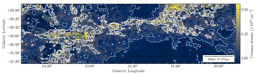
Appendix B MWISP CO observations
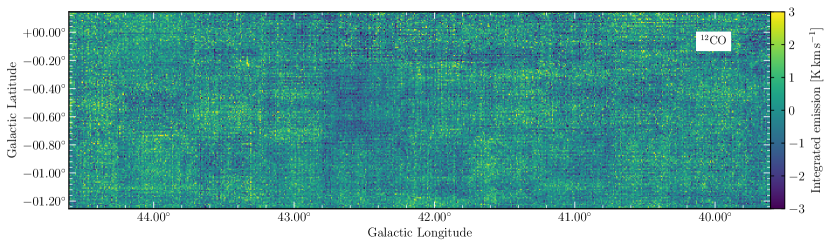
Appendix C Stellar extinctions using Gaia, 2MASS, and WISE