Mixture Proportion Estimation and PU Learning:
A Modern Approach

Abstract

Given only positive examples and unlabeled examples (from both positive and negative classes), we might hope nevertheless to estimate an accurate positive-versus-negative classifier. Formally, this task is broken down into two subtasks: (i) Mixture Proportion Estimation (MPE)—determining the fraction of positive examples in the unlabeled data; and (ii) PU-learning—given such an estimate, learning the desired positive-versus-negative classifier. Unfortunately, classical methods for both problems break down in high-dimensional settings. Meanwhile, recently proposed heuristics lack theoretical coherence and depend precariously on hyperparameter tuning. In this paper, we propose two simple techniques: Best Bin Estimation (BBE) (for MPE); and Conditional Value Ignoring Risk (CVIR), a simple objective for PU-learning. Both methods dominate previous approaches empirically, and for BBE, we establish formal guarantees that hold whenever we can train a model to cleanly separate out a small subset of positive examples. Our final algorithm (TED)ⁿ, alternates between the two procedures, significantly improving both our mixture proportion estimator and classifier.

1 Introduction

When deploying $k$-way classifiers in the wild, what can we do when confronted with data from a previously unseen class ($k+1$)? Theory dictates that learning under distribution shift is impossible absent assumptions. And yet people appear to exhibit this capability routinely. Faced with new surprising symptoms, doctors can recognize the presence of a previously unseen ailment and attempt to estimate its prevalence. Similarly, naturalists can discover new species, estimate their range and population, and recognize them reliably going forward.

To begin making this problem tractable, we might make the label shift assumption [37, 41, 29], i.e., that while the class balance $p(y)$ can change, the class conditional distributions $p(x|y)$ do not. Moreover, we might begin by focusing on the base case, where only one class has been seen previously, i.e., $k=1$. Here, we possess (labeled) positive data from the source distribution, and (unlabeled) data from the target distribution, consisting of both positive and negative instances. This problem has been studied in the literature as learning from positive and unlabeled data [8, 27] and has typically been broken down into two subtasks: (i) Mixture Proportion Estimation (MPE) where we estimate $\alpha$, the fraction of positives among the unlabeled examples; and (ii) PU-learning where this estimate is incorporated into a scheme for learning a Positive-versus-Negative (PvN) binary classifier.

Traditionally, MPE and PU-learning have been motivated by settings involving large databases where unlabeled examples are abundant and a small fraction of the total positives have been extracted. For example, medical records might be annotated indicating the presence of certain diagnoses, but the unmarked passages are not necessarily negative. This setup has also been motivated by protein and gene identification [16]. Databases in molecular biology often contain lists of molecules known to exhibit some characteristic of interest. However, many other molecules may exhibit the desired characteristic, even if this remains unknown to science.

Many methods have been proposed for both MPE [16, 12, 39, 35, 21, 4, 36, 20] and PU-learning [14, 11, 23]. However, classical MPE methods break down in high-dimensional settings [35] or yield estimators whose accuracy depends on restrictive conditions [12, 39]. On the other hand, most recent proposals either lack theoretical coherence, rely on heroic assumptions, or depend precariously on tuning hyperparameters that are, by the very problem setting, untunable. For PU learning, Elkan and Noto [16] suggest training a classifier to distinguish positive from unlabeled data followed by a rescaling procedure. Du Plessis et al. [11] suggest an unbiased risk estimation framework for PU learning. However, these methods fail badly when applied with model classes capable of overfitting and thus implementations on high-dimensional datasets rely on extensive hyperparameter tuning and additional ad-hoc heuristics that do not transport effectively across datasets.

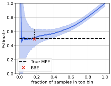
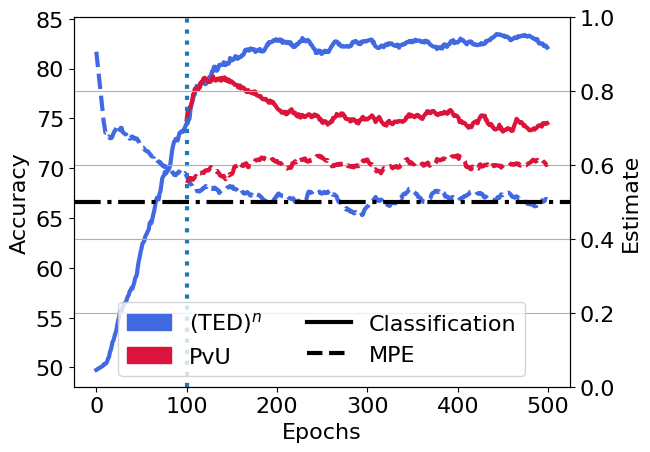
Figure 1: Illustration of proposed methods. (left) Estimate of $\bf{\alpha}$ with varying fraction of unlabeled examples in the top bin. The shaded region highlights the upper and lower confidence bounds. BBE selects the top bin that minimizes the upper confidence bound. (right) Accuracy and MPE estimate as training proceeds. Till $100$-th epoch (vertical line), we perform PvU training, i.e., warm start for (TED)ⁿ. Post $100$-th epoch, we continue with both (TED)ⁿ and PvU training. Note that (TED)ⁿ improves both classification accuracy and MPE compared to PvU training. Results with Resnet-18 on binary-CIFAR. For details and comparisons with other methods, see Sec. 6.

In this paper, we propose (i) Best Bin Estimation (BBE), an effective technique for MPE that produces consistent estimates $\widehat{\alpha}$ under mild assumptions and admits finite-sample statistical guarantees achieving the desired $O(1/\sqrt{n})$ rates; and (ii) learning with the Conditional Value Ignoring Risk (CVIR) objective, which discards the highest loss $\widehat{\alpha}$ fraction of examples on each training epoch, removing the incentive to overfit to the unlabeled positive examples. Both methods are simple to implement, compatible with arbitrary hypothesis classes (including deep networks), and dominate existing methods in our experimental evaluation. Finally, we combine the two in an iterated Transform-Estimate-Discard (TED)ⁿ framework that significantly improves both MPE estimation error and classifier error.

We build on label shift methods [29, 3, 2, 34, 17], that leverage black-box classifiers to reduce dimensionality, estimating the target label distribution as a functional of source and target push-forward distributions. While label shift methods rely on classifiers trained to separate previously seen classes, BBE is able to exploit a Positive-versus-Unlabeled (PvU) target classifier, which gives each input a score indicating how likely it is to be a positive sample. In particular, BBE identifies a threshold such that by estimating the ratio between the fractions of positive and unlabeled points receiving scores above the threshold, we obtain the mixture proportion $\alpha$.

BBE works because in practice, for many datasets, PvU classifiers, even when uncalibrated, produce outputs with near monotonic calibration diagrams. Higher scores correspond to a higher proportion of positives, and when the positive data contains a separable sub-domain, i.e., a region of the input space where only the positive distribution has support, classifiers often exhibit a threshold above which the top bin contains mostly positive examples. We show that the existence of a (nearly) pure top bin is sufficient for BBE to produce a (nearly) consistent estimate $\widehat{\alpha}$, whose finite sample convergence rates depend on the fraction of examples in the bin and whose bias depends on the purity of the bin. Crucially, we can estimate the optimal threshold from data.

We conduct a battery of experiments both to empirically validate our claim that BBE’s assumptions are mild and frequently hold in practice, and to establish the outperformance of BBE, CVIR, and (TED)ⁿ over the previous state of the art. We first motivate BBE by demonstrating that in practice PvU classifiers tend to isolate a reasonably large, reasonably pure top bin. We then conduct extensive experiments on semi-synthetic data, adapting a variety of binary classification datasets to the PU learning setup and demonstrating the superior performance of BBE and PU-learning with the CVIR objective. Moreover, we show that (TED)ⁿ, which combines the two in an iterative fashion, improves significantly over previous methods across several architectures on a range of image and text datasets.

2 Related Work

Research on MPE and PU learning date to [9, 8, 27] (see review by [5]). Elkan and Noto [16] first proposed to leverage a PvU classifier to estimate the mixture proportion. Du Plessis and Sugiyama [13] propose a different method for estimating the mixture coefficient based on Pearson divergence minimization. While they do not require a PvU classifier, they suffer the same shortcoming. Both methods require that the positive and negative examples have disjoint support. Our requirements are considerably milder. Blanchard et al. [6] observe that without assumptions on the underlying positive and negative distributions, the mixture proportion is not identifiable. Furthermore, [6] provide an irreducibility condition that identifies $\alpha$ and propose an estimator that converges to the true $\alpha$. While their estimator can converge arbitrarily slowly, Scott [39] showed faster convergence ($\mathcal{O}(1/\sqrt{n})$) under stronger conditions. Unfortunately, despite its appealing theoretical properties Blanchard et al. [6]’s estimator is computationally infeasible. Building on Blanchard et al. [6], Sanderson and Scott [38] and Scott [39] proposed estimating the mixture proportion from a ROC curve constructed for the PvU classifier. However, when the PvU classifier is not perfect, these methods are not clearly understood. Ramaswamy et al. [35] proposed the first computationally feasible algorithm for MPE with convergence guarantees to the true proportion. Their method KM, requires embedding distributions onto an RKHS. However, their estimator underperforms on high dimensional datasets and scales poorly with large datasets. Bekker and Davis [4] proposed TIcE, hoping to identify a positive subdomain in the input space using decision tree induction. This method also underperforms in high-dimensional settings.

In the most similar works, Jain et al. [21] and Ivanov [20] explore dimensionality reduction using a PvU classifier. Both methods estimate $\alpha$ through a procedure operating on the PvU classifier’s output. However, neither methods has provided theoretical backing. [20] concede that their method often fails and returns a zero estimate, requiring that they fall back to a different estimator. Moreover while both papers state that their method require the Bayes-optimal PvU classifier to identify $\alpha$ in the transformed space, we prove that even when hypothesis class is well specified for PvN learning, PvU training can fail to recover the Bayes-optimal scoring function. Furthermore, we also show that the heuristic estimator in Scott [39] can be thought of as using PvU classifier for dimensionality reduction. While this heuristic is similar to our estimator in spirit, we show that the functional form of their estimator is different from ours and note that their heuristic enjoys no theoretical guarantee. By contrast, our estimator BBE is theoretically coherent under mild conditions and outperforms all of these methods empirically.

Given $\alpha$, Elkan and Noto [16] propose a transformation via Bayes rule to obtain the PvN classifier. They also propose a weighted objective, with weights given by the PvU classifier. Other propose unbiased risk estimators [14, 11] which require the mixture proportion $\alpha$. Du Plessis et al. [14] proposed an unbiased estimator with non-convex loss functions satisfying a specific symmetric condition, and subsequently Du Plessis et al. [11] generalized it to convex loss functions (denoted uPU in our experiments). in our experiments. Noting the problem of overfitting in modern overparameterized models, Kiryo et al. [23] propose a regularized extension that clips the loss on unlabeled data to zero. This is considered the current state-of-the-art in PU literature (denoted nnPU in our experiments). More recently, Ivanov [20] proposed DEDPUL, which finetunes the PvU classifiers using several heuristics, Bayes rule, and Expectation Maximization (EM). Since their method only applies a post-processing procedure, they rely on a good domain discriminator classifier in the first place and several hyperparameters for their heuristics. Several classical methods attempt to learn weights that identify reliable negative examples [30, 28, 26, 31, 44]. However, these earlier methods have not been successful with modern deep learning models.

3 Problem Setup

By $\left|\!\left|\cdot\right|\!\right|$ and $\langle\cdot,\cdot\rangle$, we denote the Euclidean norm and inner product, respectively. For a vector $v\in\mathbb{R}^{d}$, we use $v_{j}$ to denote its $j^{\text{th}}$ entry, and for an event $E$, we let $\mathbb{I}\left[E\right]$ denote the binary indicator of the event. By $\left\lvert A\right\rvert$, we denote the cardinality of set $A$. Let $\mathcal{X}\in\mathbb{R}^{d}$ be the input space and $\mathcal{Y}=\{-1,+1\}$ be the output space. Let $\mathrm{P}:\mathcal{X}\times\mathcal{Y}\to[0,1]$ be the underlying joint distribution and let $p$ denote its corresponding density.

Let $\mathrm{P}_{p}$ and $\mathrm{P}_{n}$ be the class-conditional distributions for positive and negative class and $p_{p}(x)=p(x|y=+1)$ and $p_{n}(x)=p(x|y=-1)$ be the corresponding class-conditional densities. $\mathrm{P}_{u}$ denotes the distribution of the unlabeled data and $p_{u}$ denotes its density. Let $\alpha\in[0,1]$ be the fraction of positives among the unlabeled population, i.e., $\mathrm{P}_{u}=\alpha\mathrm{P}_{p}+(1-\alpha)\mathrm{P}_{n}$. When learning from positive and unlabeled data, we obtain i.i.d. samples from the positive (class-conditional) distribution, which we denote as $X_{p}=\{x_{1},x_{2},\ldots,x_{n_{p}}\}\sim\mathrm{P}_{p}^{n_{p}}$ and i.i.d samples from unlabeled distribution as $X_{u}=\{x_{n_{p}+1},x_{n_{p}+2},\ldots,x_{n_{p}+n_{u}}\}\sim\mathrm{P}_{u}^{n_{u}}$.

MPE is the problem of estimating $\alpha$. Absent assumptions on $\mathrm{P}_{p}$, $\mathrm{P}_{n}$ and $\mathrm{P}_{u}$, the mixture proportion $\alpha$ is not identifiable [6]. Indeed, if $\mathrm{P}_{u}=\alpha\mathrm{P}_{p}+(1-\alpha)\mathrm{P}_{n}$, then any alternate decomposition of the form $\mathrm{P}_{u}=(\alpha-\gamma)\mathrm{P}_{p}+(1-\alpha+\gamma)\mathrm{P}_{n}^{\prime}$, for $\gamma\in[0,\alpha)$ and $\mathrm{P}_{n}^{\prime}=(1-\alpha+\gamma)^{-1}(\gamma\mathrm{P}_{p}+(1-\alpha)\mathrm{P}_{n})$, is also valid. Since we do not observe samples from the distribution $\mathrm{P}_{n}$, the parameter $\alpha$ is not identifiable. Blanchard et al. [6] formulate an irreducibility condition under which $\alpha$ is identifiable. Intuitively, the condition restricts $\mathrm{P}_{n}$ to ensure that it can not be a (non-trivial) mixture of $\mathrm{P}_{p}$ and any other distribution. While this irreducibility condition makes $\alpha$ identifiable, in the worst-case, the parameter $\alpha$ can be difficult to estimate and any estimator must suffer an arbitrarily slow rate of convergence [6]. In this paper, we propose mild conditions on the PvU classifier that make $\alpha$ identifiable and allows us to derive finite-sample convergence guarantees.

With PU learning, the aim is to learn a classifier $f:\mathcal{X}\to[0,1]$ to approximate $p(y=+1|x)$. We assume that we are given a loss function $\ell:[0,1]\times\mathcal{Y}\to\mathbb{R}$, such that $\ell(z,y)$ is the loss incurred by predicting $z$ when the true label is $y$. For a classifier $f$ and a sampled set $X=\{x_{1},x_{2},\ldots,x_{n}\}$, we let $\widehat{L}^{+}(f;X)=\sum_{i=1}^{n}\ell(f(x_{i}),+1)/n$ denote the loss when predicting the samples as positive and $\widehat{L}^{-}(f;X)=\sum_{i=1}^{n}\ell(f(x_{i}),-1)/n$ the loss when predicting the samples as negative. For a sample set $X$ each with true label $y$, we define 0-1 error as $\widehat{\mathcal{E}}^{y}(f;X)=\sum_{i=1}^{n}\mathbb{I}\left[y(f(x_{i})-t)\leq 0\right]/n$ for some predefined threshold $t$ . Unless stated otherwise, the threshold is assumed to be $0.5$.

4 Mixture Proportion Estimation

Algorithm 1 Best Bin Estimation (BBE)

0:  : Validation positive ($X_{p}$) and unlabeled ($X_{u}$) samples. Blackbox model classifier $\widehat{f}:\mathcal{X}\to[0,1]$. Hyperparameter $0<\delta,\gamma<1$.

1:  $Z_{p},Z_{u}=f(X_{p}),f(X_{u})$.

2:  $\widehat{q}_{u}(z),\widehat{q}_{p}(z)=\frac{\sum_{z_{i}\in Z_{p}}\mathbb{I}\left[z_{i}\geq z\right]}{n_{p}},\frac{\sum_{z_{i}\in Z_{u}}\mathbb{I}\left[z_{i}\geq z\right]}{n_{u}}$ for all $z\in[0,1]$.

3:  Estimate $\widehat{c}\vcentcolon=\operatorname*{arg\,min}_{c\in[0,1]}\left(\frac{\widehat{q}_{u}(c)}{\widehat{q}_{p}(c)}+\frac{1+\gamma}{\widehat{q}_{p}(c)}\left(\sqrt{\frac{\log(4/\delta)}{2n_{u}}}+\sqrt{\frac{\log(4/\delta)}{2n_{p}}}\right)\right)\,$.

3:  : $\widehat{\alpha}\vcentcolon=\frac{\widehat{q}_{u}(\widehat{c})}{\widehat{q}_{p}(\widehat{c})}$

In this section, we introduce BBE, a new method that leverages a blackbox classifier $f$ to perform MPE and establish convergence guarantees. All proofs are relegated to App. B. To begin, we assume access to a fixed classifier $f$. For intuition, you may think of $f$ as a PvU classifer trained on some portion fo the positive and unlabeled examples. In Sec. 5, we discuss other ways to obtain a suitable classifier from PU data.

We now introduce some additional notation. Assume $f$ transforms an input $x\in\mathcal{X}$ to $z\in[0,1]$, i.e., $z=f(x)$. For given probability density function $p$ and a classifier $f$, define a function $q(z)=\int_{A_{z}}p(x)dx$, where $A_{z}=\{x\in\mathcal{X}:f(x)\geq z\}$ for all $z\in[0,1]$. Intuitively, $q(z)$ captures the cumulative density of points in a top bin, the proportion of input domain that is assigned a value larger than $z$ by the classifier $f$ in the transformed space. We now define an empirical estimator $\widehat{q}(z)$ given a set $X=\{x_{1},x_{2},\ldots,x_{n}\}$ sampled iid from $p(x)$. Let $Z=f(X)$. Define $\widehat{q}(z)=\sum_{i=1}^{n}\mathbb{I}\left[z_{i}\geq z\right]/{n}$. For each pdf $p_{p}$, $p_{n}$ and $p_{u}$, we define $q_{p}$, $q_{n}$ and $q_{u}$ respectively.

Without any assumptions on the underlying distribution and the classifier $f$, we aim to estimate $\alpha^{*}=\min_{c\in[0,1]}q_{u}(c)/q_{p}(c)$ with BBE. Later, under one mild assumption that empirically holds across numerous PU datasets, we show that $\alpha^{*}=\alpha$, i.e., $\alpha^{*}$ matches the true mixture proportion $\alpha$.

Our procedure proceeds as follows: First, given a held-out dataset of positive ($X_{p}$) and unlabeled examples ($X_{u}$), we push all examples through the classifier $f$ to obtain one-dimensional outputs $Z_{p}=f(X_{p})$ and $Z_{u}=f(X_{u})$. Next, with $Z_{p}$ and $Z_{u}$, we estimate $\widehat{q}_{p}$ and $\widehat{q}_{u}$. Finally, we return the ratio $\widehat{q}_{u}(\widehat{c})/\widehat{q}_{p}(\widehat{c})$ at $\widehat{c}$ that minimizes the upper confidence bound (calculated using Lemma 1) at a pre-specified level $\delta$ and a fixed parameter $\gamma\in(0,1)$. Our method is summarized in Algorithm 1. For theoretical guarantees, we multiply the confidence bound term with $1+\gamma$ for a small positive constant $\gamma$. Refer to App. B.1 for details. We now show that the proposed estimator comes with the following guarantee:

Theorem 1.

Define $c^{*}=\operatorname*{arg\,min}_{c\in[0,1]}q_{u}(c)/q_{p}(c)$. For $\min(n_{p},n_{u})\geq\frac{2\log(4/\delta)}{q_{p}(c^{*})}$ and for every $\delta>0$, the mixture proportion estimator $\widehat{\alpha}$ defined in Algorithm 1 satisfies with probability $1-\delta$:

$$\left\lvert\widehat{\alpha}-\alpha^{*}\right\rvert\leq\frac{c}{q_{p}(c^{*})}\left(\sqrt{\frac{\log(4/\delta)}{n_{u}}}+\sqrt{\frac{\log(4/\delta)}{n_{p}}}\right)\,,$$

for some constant $c\geq 0$.

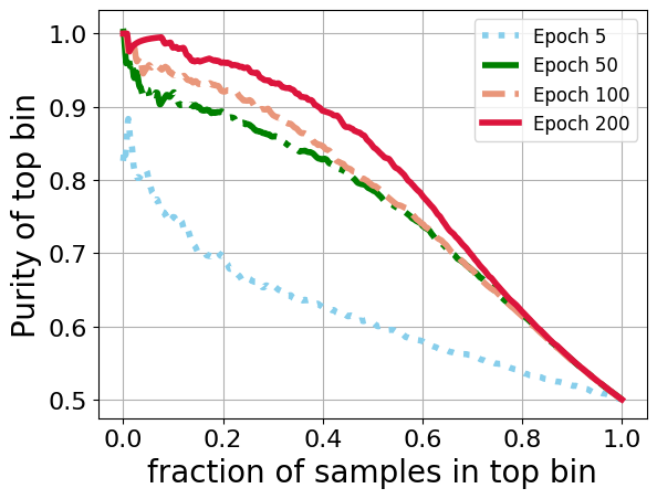
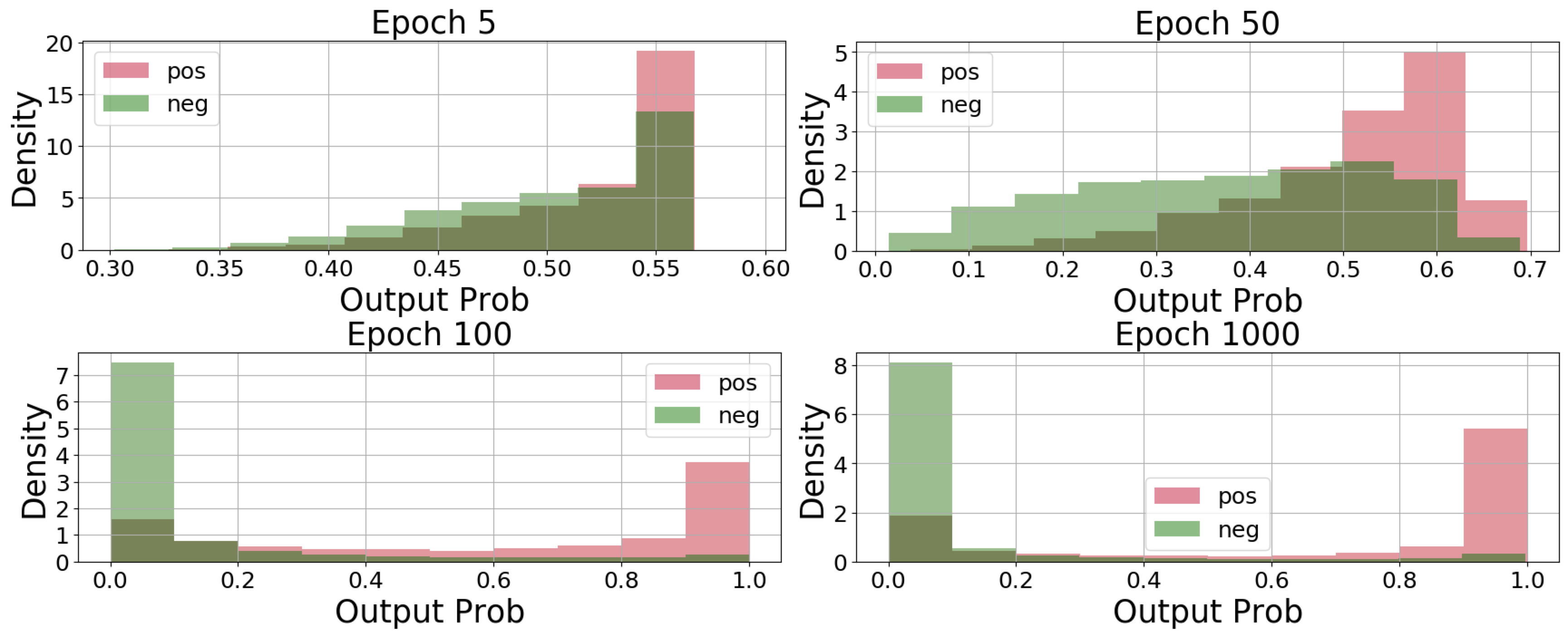
Figure 2: (a) Purity and size (in terms of fraction of unlabeled samples) in the top bin and (b) Distribution of predicted probabilities (of being positive) for unlabeled training data as training proceeds with (TED)ⁿ. Results with ResNet-18 on binary-CIFAR. As in Fig. 1, we fix $W$ at $100$. In App. G.4, we show that as PvU training proceeds, the purity of top bin degrades and the distribution of predicted probabilities of positives and negatives become less and less separable.

Theorem 1 shows that with high probability, our estimate is close to $\alpha^{*}$. The proof of the theorem is based on the following confidence bound inequality:

Lemma 1.

For every $\delta>0$, with probability at least $1-\delta$, we have for all $c\in[0,1]$

$$\left\lvert\frac{\widehat{q}_{u}(c)}{\widehat{q}_{p}(c)}-\frac{q_{u}(c)}{q_{p}(c)}\right\rvert\leq\frac{1}{\widehat{q}_{p}(c)}\left(\sqrt{\frac{\log(4/\delta)}{2n_{u}}}+\frac{q_{u}(c)}{q_{p}(c)}\sqrt{\frac{\log(4/\delta)}{2n_{p}}}\right)\,.$$

Now, we discuss the convergence of our estimator to the true mixture proportion $\alpha$. Since, $p_{u}(x)=\alpha p_{p}(x)+(1-\alpha)p_{n}(x)$, for all $x\in\mathcal{X}$, we have $q_{u}(z)=\alpha q_{p}(z)+(1-\alpha)q_{n}(z)$, for all $z\in[0,1]$.

Corollary 1.

Define $c^{*}=\operatorname*{arg\,min}_{c\in[0,1]}q_{n}(c)/q_{p}(c)$. Assume $\min(n_{p},n_{u})\geq\frac{2\log(4/\delta)}{q_{p}(c^{*})}$. For every $\delta>0$, $\widehat{\alpha}$ (in Algorithm 1) satisfies with probability $1-\delta$:

$$\alpha-\frac{c_{1}}{q_{p}(c^{*})}\left(\sqrt{\frac{\log(4/\delta)}{n_{u}}}+\sqrt{\frac{\log(4/\delta)}{n_{p}}}\right)\leq\widehat{\alpha}\,,\text{and}$$

$$\widehat{\alpha}\leq\alpha+(1-\alpha)\frac{q_{n}(c^{*})}{q_{p}(c^{*})}+\frac{c_{2}}{q_{p}(c^{*})}\left(\sqrt{\frac{\log(4/\delta)}{n_{u}}}+\sqrt{\frac{\log(4/\delta)}{n_{p}}}\right)\,,$$

for some constant $c_{1},c_{2}\geq 0$.

As a corollary to Theorem 1, we show that our estimator $\widehat{\alpha}$ converges to the true $\alpha$ with convergence rate $\min(n_{p},n_{u})^{-1/2}$, as long as there exist a threshold $c_{f}\in(0,1)$ such that $q_{p}(c_{f})\geq\epsilon_{p}$ and $q_{n}(c_{f})=0$ for some constant $\epsilon_{p}>0$. We refer to this condition as the pure positive bin property.

Note that in a more general case, our bound in Corollary 1 captures the tradeoff due to the proportion of negative examples in the top bin (bias) versus the proportion of positives in the top bin (variance).

Empirical Validation We now empirically validate the positive pure top bin property (Fig. 2). We observe that as PvU training proceeds, purity of the top bin improves for a fixed fraction of samples in the top bin. Moreover, this behavior becomes more pronounced when learning a PvU classifier with the CVIR objective proposed in the following section.

Comparison with existing methods Due to the intractability of Blanchard et al. [6] estimator, Scott [39] implements a heuristic based on identifying a point on the AUC curve such that the slope of the line segment between this point and (1,1) is minimized. While this approach is similar in spirit to our BBE method, there are some striking differences. First, the heuristic estimator in Scott [39] provides no theoretical guarantees, whereas we provide guarantees that BBE will converge to the best estimate achievable over all choices of the bin size and provide consistent estimates whenever a pure top bin exists. Second, while both estimates involve thresholds, the functional form of the estimates are different. Corroborating theoretical results of BBE, we observe that the choices in BBE create substantial differences in the empirical performance as observed in App. C. We work out details of comparison between Scott [39] heuristic and BBE in App. C.

On the other hand, recent works [21, 20] that use PvU classifier for dimensionality reduction, discuss Bayes optimality of the PvU classifier (or its one-to-one mapping) as a sufficient condition to preserve $\alpha$ in transformed space. By contrast, we show that the milder pure positive bin property is sufficient to guarantee consistency and achieve $\mathcal{O}(1/\sqrt{n})$ rates. Furthermore, in a simple toy setup in App. D, we show that even when the hypothesis class is well specified for PvN learning, it will not in general contain the Bayes optimal PvU classifier and thus PvU training will not recover the Bayes-optimal scoring function, even in population. Contrarily, we show that any monotonic mapping of the Bayes-optimal PvU scoring function induces a positive pure top bin property. We leave further theoretical investigations concerning conditions under which a pure positive top bin arises to future work.

5 PU-Learning

Algorithm 2 PU learning with Conditional Value Ignoring Risk (CVIR) objective

0:  : Labeled positive training data ($X_{p}$) and unlabeled training samples ($X_{u}$). Mixture proportion estimate $\alpha$.

1:  Initialize a training model $f_{\theta}$ and an stochastic optimization algorithm $\mathcal{A}$.

2:  $X_{n}\vcentcolon=X_{u}$.

3:  while training error $\widehat{\mathcal{E}}^{+}(f_{\theta};X_{p})+\widehat{\mathcal{E}}^{-}(f_{\theta};X_{n})$ is not converged do

4:     Rank samples $x_{u}\in X_{u}$ according to their loss values $\ell(f_{\theta}(x_{u}),-1)$.

5:     $X_{n}\vcentcolon=X_{u,1-\alpha}$ where $X_{u,1-\alpha}$ denote the lowest ranked $1-\alpha$ fraction of samples.

6:     Shuffle $(X_{p},X_{n})$ into $B$ mini-batches. With $(X_{p}^{i},X_{n}^{i})$ we denote $i$-th mini-batch.

7:     for  $i=1$ to $B$ do

8:        Set the gradient $\nabla_{\theta}\left[\alpha\cdot\widehat{L}^{+}(f_{\theta};X_{p}^{i})+(1-\alpha)\cdot\widehat{L}^{-}(f_{\theta};X_{n}^{i})\right]$ and update $\theta$ with algo. $\mathcal{A}$.

9:     end for

10:  end while

10:  : Trained classifier $f_{\theta}$

Given positive and unlabeled data, we hope not only to identify $\alpha$, but also to obtain a classifier that distinguishes effectively between positive and negative samples. In supervised learning with separable data (e.g., cleanly labeled image data), overparameterized models generalize well even after achieving near-zero training error. However, with PvU training over-parameterized models can memorize the unlabeled positives, assigning them confidently to the negative class, which can severely hurt generalization on PN data [43]. Moreover, while unbiased losses exist that estimate the PvN loss given PU data and the mixture proportion $\alpha$, this unbiasedness only holds before the loss is optimized, and becomes ineffective with powerful deep learning models capable of memorization.

A variety of heuristics, including ad-hoc early stopping criteria, have been explored [20], where training proceeds until the loss on unseen PU data ceases to decrease. However, this approach leads to severe under-fitting (results in App. G.2). On the other hand, by regularizing the loss function, nnPU Kiryo et al. [23] mitigates overfitting issues due to memorization.

However, we observe that nnPU still leaves a substantial accuracy gap when compared to a model trained just on the positive and negative (from the unlabeled) data (ref. experiment in App. G.1). This leads us to ask the following question: can we improve performance over nnPU of a model just trained with PU data and bridge this gap? In an ideal scenario, if we could identify and remove all the positive points from the unlabeled data during training then we can hope to achieve improved performance over nnPU. Indeed, in practice, we observe that in the initial stages of PvU training, the model assigns much higher scores to positives than to negatives in the unlabeled data (Fig. 2(b)).

Inspired by this observation, we propose CVIR, a simple yet effective objective for PU learning. Below, we present our method assuming an access to the true MPE. Later, we combine BBE with CVIR optimization, yielding (TED)ⁿ, an alternating optimization that significantly improves both the BBE estimates and the PvU classifier.

Given a training set of positives $X_{p}$ and unlabeled $X_{u}$ and the mixture proportion $\alpha$, we begin by ranking the unlabeled data according the predicted probability (of being positive) by our classifier. Then, in every epoch of training, we create a (temporary) set of provisionally negative samples $X_{n}$ by removing $\alpha$ fraction of the unlabeled samples currently scored as most positive. Next, we update our classifier by minimize the loss on the positives $X_{p}$ and provisional negatives $X_{n}$ by treating them as negatives. We repeat this procedure until the training error on $X_{p}$ and $X_{n}$ converges. Likewise nnPU, note that this procedure does not need early stopping. Summary in Algorithm 2.

In App. E, we justify our loss function in the scenario when the positives and negatives are separable. For a more general scenario, we show that each step of our alternating procedure in CVIR cannot increase the population loss and hence, CVIR can only improve (or plateau) after every iteration.

(TED)ⁿ Integrating BBE and CVIR We are now ready to present our algorithm Transfer, Estimate and Discard (TED)ⁿ that combines BBE and CVIR objective.

Algorithm 3 Transform-Estimate-Discard (TED)ⁿ

0:  : Positive data ($X_{p}$) and unlabeled samples ($X_{u}$). Hyperparameter $W,\delta$.

1:  Initialize a training model $f_{\theta}$ and an stochastic optimization algorithm $\mathcal{A}$.

2:  Randomly split positive and unlabeled data into training $X^{1}_{p},X^{1}_{u}$ and hold-out set ($X^{2}_{p},X^{2}_{u}$).

3:  $X^{1}_{n}\vcentcolon=X^{1}_{u}$. {// Warm start with domain discrimination training}

4:  for  $i=1$ to $W$ do

5:     Shuffle $(X_{p}^{1},X_{n}^{1})$ into $B$ mini-batches. With $({X^{1}_{p}}^{i},{X^{1}_{n}}^{i})$ we denote $i$-th mini-batch.

6:     for  $i=1$ to $B$ do

7:        Set the gradient $\nabla_{\theta}\left[\widehat{L}^{+}(f_{\theta};{X^{1}_{p}}^{i})+\widehat{L}^{-}(f_{\theta};{X^{1}_{n}}^{i})\right]$ and update $\theta$ with algorithm $\mathcal{A}$.

8:     end for

9:  end for

10:  while training error $\widehat{\mathcal{E}}^{+}(f_{\theta};X^{1}_{p})+\widehat{\mathcal{E}}^{-}(f_{\theta};X^{1}_{n})$ is not converged do

11:     Estimate $\widehat{\alpha}$ using Algorithm 1 with $(X^{2}_{p},X^{2}_{u})$ and $f_{\theta}$ as input.

12:     Rank samples $x_{u}\in X^{1}_{u}$ according to their loss values $l(f_{\theta}(x_{u}),-1)$.

13:     $X^{1}_{n}\vcentcolon=X^{1}_{u,1-\widehat{\alpha}}$ where $X^{1}_{u,1-\widehat{\alpha}}$ denote the lowest ranked $1-\widehat{\alpha}$ fraction of samples.

14:     Train model $f_{\theta}$ for one epoch on $(X^{1}_{p},X^{1}_{n})$ as in Lines 4-7.

15:  end while

15:  : Trained classifier $f_{\theta}$

First, we observe the interaction between BBE and CVIR objective. If we have an accurate mixture proportion estimate, then it leads to improved classifier, in particular, we reject accurate number of prospective positive samples from unlabeled. Consequently, updating the classifier to minimize loss on positive versus retained unlabeled improves purity of top bin. This leads to an obvious alternating procedure where at each epoch, we first use BBE to estimate $\widehat{\alpha}$ and then update the classifier with CVIR objective with $\widehat{\alpha}$ as input. We repeat this until training error has not converged. Our method is summarized in Algorithm 3.

Note that we need to warm start with PvU (positive versus negative) training, since in the initial stages mixture proportion estimate is often close to 1 rejecting all the unlabeled examples. However, in next section, we show that our procedure is not sensitive to the choice of number of warm start epochs and in a few cases with large datasets, we can even get away without warm start (i.e., $W=0$) without hurting the performance. Moreover, recall that our aim is to distinguish positive versus negative examples among the unlabeled set where the proportion of positives is determined by the true mixture proportion $\alpha$. However, unlike CVIR, we do not re-weight the losses in (TED)ⁿ. While true MPE $\alpha$ is unknown, one natural choice is to use the estimate $\widehat{\alpha}$ at each iteration. However, in our initial experiments, we observed that re-weighted objective with estimate $\widehat{\alpha}$ led to comparatively poor classification performance due to presence of bias in estimate $\widehat{\alpha}$ in the initial iterations. We note that for deep neural networks (for which model mis-specification is seldom a prominent concern) and when the underlying classes are separable (as with most image datasets), it is known that importance weighting has little to no effect on the final classifier [7]. Therefore, we may not need importance-reweighting with (TED)ⁿ on separable datasets. Consequently, following earlier works [23, 11] we do not re-weight the loss with our (TED)ⁿ procedure. In future work, a simple empirical strategy can be explored where we first obtain an estimate of $\widehat{\alpha}$ by running the full (TED)ⁿ procedure till convergence and then discarding the (TED)ⁿ classifier, we use estimate $\widehat{\alpha}$ to train a fresh classifier with CVIR procedure.

Finally, we discuss an important distinction with Dedpul which is also an alternating procedure. While in our algorithm, after updating mixture proportion estimate we retrain the classifier, Dedpul fixes the classifier, obtains output probabilities and then iteratively updates the mixture proportion estimate (prior) and output probabilities (posterior). Dedpul doesn’t re-train the classifier.

6 Experiments

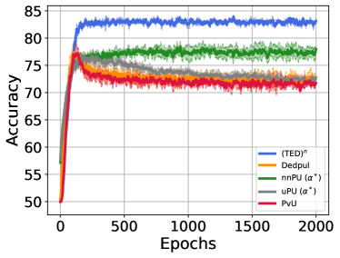
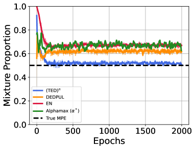
Figure 3: Epoch wise results with ResNet-18 trained on binary-CIFAR when $\alpha$ is $0.5$. Parallel results on other datasets and architectures in App. G.3. For both classification and MPE, (TED)ⁿ substantially improves over existing methods. Additionally, (TED)ⁿ maintains the superior performance till convergence removing the need for early stopping. Results aggregated over 3 seeds.

Having presented our PU learning and MPE algorithms, we now compare their performance with other methods empirically. We mainly focus on vision and text datasets in our experiments. We include results on UCI datasets in App. G.7.

Datasets and Evaluation We simulate PU tasks on CIFAR-10 [24], MNIST [25], and IMDb sentiment analysis [32] datasets. We consider binarized versions of CIFAR-10 and MNIST. On CIFAR-10 dataset, we consider two classification problems: (i) binarized CIFAR, i.e., first 5 classes vs rest; (ii) Dog vs Cat in CIFAR. Similarly, on MNIST, we consider: (i) binarized MNIST, i.e., digits 0-4 vs 5-9; (ii) MNIST17, i.e., digit 1 vs 7. IMDb dataset is binary. For MPE, we use a held out PU validation set. To evaluate PU classifiers, we calculate accuracy on held out positive versus negative dataset. For baselines that suffer from issues due to overfitting on unlabeled data, we report results with an oracle early stopping criterion. In particular, we report the accuracy averaged over $10$ iterations of the best performing model as evaluated on positive versus negative data. Note that we use this oracle stopping criterion only for previously proposed methods and not for methods proposed in this work. This allows us to compare (TED)ⁿ with the best performance achievable by previous methods that suffer from over-fitting issues. With nnPU and (TED)ⁿ, we report average accuracy over $10$ iterations of the final model.

Architectures For CIFAR datasets, we consider (fully connected) multilayer perceptrons (MLPs) with ReLU activations, all convolution nets [40], and ResNet18 [19]. For MNIST, we consider multilayer perceptrons (MLPs) with ReLU activations For the IMDb dataset, we fine-tune an off-the-shelf uncased BERT model [10, 42]. We did not tune hyperparameters or the optimization algorithm—instead we use the same benchmarked hyperparameters and optimization algorithm for each dataset. For our method, we use cross-entropy loss. For uPU and nnPU, we use Adam [22] with sigmoid loss. We provide additional details about the datasets and architectures in App. F.

Dataset	Model	(TED)n	BBE∗	DEDPUL∗	AlphaMax∗	EN∗	KM2	TiCE
Binarized CIFAR	ResNet	$\mathbf{0.026}$	$0.091$	$0.091$	$0.125$	$0.192$
	All Conv	$0.042$	$\mathbf{0.037}$	$0.052$	$0.09$	$0.221$	$0.168$	$0.251$
	MLP	$0.225$	$0.177$	$\mathbf{0.138}$	$0.3$	$0.372$
CIFAR Dog vs Cat	ResNet	$\mathbf{0.078}$	$0.176$	$0.170$	$0.17$	$0.226$	$0.331$	$0.286$
	All Conv	$\mathbf{0.066}$	$0.128$	$0.115$	$0.19$	$0.250$
Binarized MNIST	MLP	$\mathbf{0.024}$	$0.032$	$0.031$	$0.090$	$0.080$	$0.029$	$0.056$
MNIST17	MLP	$\mathbf{0.003}$	$0.023$	$0.021$	$0.075$	$0.028$	$0.022$	$0.043$
IMDb	BERT	$\mathbf{0.008}$	$0.011$	$0.016$	$0.07$	$0.12$	-	-

Table 1: Absolute estimation error when $\alpha$ is 0.5. "*" denote oracle early stopping as defined in Sec. 6. (TED)ⁿ significantly reduces estimation error when compared with existing methods. Results reported by aggregating absolute error over 10 epochs and 3 seeds. For aggregate numbers with standard deviation see App. G.6.

Dataset	Model	(TED)n (unknown $\alpha$)	CVIR (known $\alpha$)	PvU∗ (known $\alpha$)	DEDPUL∗ (unknown $\alpha$)	nnPU (known $\alpha$)	uPU∗ (known $\alpha$)
Binarized CIFAR	ResNet	$\mathbf{82.7}$	$82.3$	$76.9$	$77.1$	$77.2$	$76.7$
	All Conv	$77.9$	$\mathbf{78.1}$	$75.8$	$77.1$	$73.4$	$72.5$
	MLP	$64.2$	$\mathbf{66.9}$	$61.6$	$62.6$	$63.1$	$64.0$
CIFAR Dog vs Cat	ResNet	$\mathbf{75.2}$	$73.3$	$67.3$	$67.0$	$71.8$	$68.8$
	All Conv	$\mathbf{73.0}$	$71.7$	$70.5$	$69.2$	$67.9$	$67.5$
Binarized MNIST	MLP	$95.6$	$\mathbf{96.3}$	$94.2$	$94.8$	$96.1$	$95.2$
MNIST17	MLP	$\mathbf{98.7}$	$\mathbf{98.7}$	$96.9$	$97.7$	$98.4$	$98.4$
IMDb	BERT	$\mathbf{87.6}$	$87.4$	$86.1$	$87.3$	$86.2$	$85.9$

Table 2: Accuracy for PvN classification with PU learning. "*" denote oracle early stopping as defined in Sec. 6. Results reported by aggregating over 10 epochs and 3 seeds. Both CVIR (with known MPE) and (TED)ⁿ (with unknown MPE) significantly improve over previous baselines with oracle early stopping and known MPE. For aggregate numbers with standard deviation see App. G.6.

Mixture Proportion Estimation First, we discuss results for MPE (Table 1). We compare our method with KM2, TiCE, DEDPUL, AlphaMax and EN. Following earlier works [20, 35], we reduce datasets to $50$ dimensions with PCA for KM2 and TiCE. We use existing implementation for other methods. For BBE, DEDPUL and Alphamax, we use the same PvU classifier as input. On CIFAR datasets, convolutional classifier based estimators significantly outperform KM2 and TiCE. In contrast, the performance of KM2 is comparable to DEDPUL on MNIST datasets. On all datasets, (TED)ⁿ achieves lowest estimation error. With the same blackbox classifier obtained with oracle early stopping, BBE performs similar or better than best alternate(s). Since overparamterized models start memorizing unlabeled samples negatives, the quality of MPE degrades substantially as PvU training proceeds for all methods but (TED)ⁿ as in Fig. 3 (epoch-wise results for on other tasks in App. G.3).

Classification with known MPE Now, we discuss results for classification with known $\alpha$. We compare our method with uPU, nnPU, DEDPUL and PvU training. Although, we solve both MPE and classification, some comparison methods do not. Ergo, we compare our classification algorithm with known MPE (Algorithm 2).

To begin, first we note that nnPU and PvU training with CVIR doesn’t need early stopping. For all other methods, we report the best performance dictated by the aformentioned oracle stopping criterion. On all datasets, PvU training with CVIR leads to improved classification performance when compared with alternate approaches (Table 2). Moreover, as training proceeds (Fig. 3), the performance of DEDPUL, PvU training and uPU substantially degrade. We repeated experiments with the early stopping criterion mentioned in DEDPUL (App. G.2), however, their early stopping criterion is too pessimistic resulting in poor results due to under-fitting.

Classification with unknown MPE Finally, we evaluate (TED)ⁿ, our alternating procedure for MPE and PU learning. Across many tasks, we observe substantial improvements over existing methods. Note that these improvements often are over an oracle early stopping baselines highlighting significance of our procedure.

In App. G.5, we show that our procedure is not sensitive to warm start epochs W, and in many tasks with $W=0$, we observe minor-to-no differences in the performance of (TED)ⁿ. While for the experiments in this section, we used fixed $W=100$, in the Appendix we show behavior with varying W. We also include ablations with different mixture proportions $\alpha$.

7 Conclusion and Future Work

In this paper, we proposed two practical algorithms, BBE (for MPE) and CVIR optimization (for PU learning). Our methods outperform others empirically and BBE’s mixture proportion estimates leverage black box classifiers to produce (nearly) consistent estimates with finite sample convergence guarantees whenever we possess a classifier with a (nearly) pure top bin. Moreover, (TED)ⁿ combines our procedures in an iterative fashion, achieving further gains. An important next direction is to extend our work to the multiclass problem [38], bridging work on label shift and PU learning. Here, we imagine that a deployed $k$-way classifier may encounter not only label shift among previously seen classes ([29, 17]) but also, potentially, instances from one previously unseen class. We also plan to investigate distributional properties under which we can hope to reliably or approximately satisfy the pure positive bin property with an off-the-shelf classifier trained on PvU data. While we improve significantly over previous PU methods, there is still a gap between (TED)ⁿ’s performance and PvN training. We hope that our work can open a pathway towards further narrowing this gap.

Appendix A Appendix

Appendix B Proofs from Sec. 4

Proof of Lemma 1.

The proof primarily involves using DKW inequality [15] on $\widehat{q}_{u}(c)$ and $\widehat{q}_{p}(c)$ to show convergence to their respective means $q_{u}(c)$ and $q_{p}(c)$. First, we have

$$\left\lvert\frac{\widehat{q}_{u}(c)}{\widehat{q}_{p}(c)}-\frac{q_{u}(c)}{q_{p}(c)}\right\rvert =\frac{1}{\widehat{q}_{u}(c)\cdot q_{u}(c)}\left\lvert\widehat{q}_{u}(c)\cdot q_{p}(c)-q_{p}(c)\cdot q_{u}(c)+q_{p}(c)\cdot q_{u}(c)-\widehat{q}_{p}(c)\cdot q_{u}(c)\right\rvert$$

$$\leq\frac{1}{\widehat{q}_{p}(c)}\left\lvert\widehat{q}_{u}(c)-q_{u}(c)\right\rvert+\frac{q_{u}(c)}{\widehat{q}_{p}(c)\cdot q_{u}(c)}\left\lvert\widehat{q}_{p}(c)-q_{p}(c)\right\rvert\,.$$ (1)

Using DKW inequality, we have with probability $1-\delta$: $\left\lvert\widehat{q}_{p}(c)-q_{p}(c)\right\rvert\leq\sqrt{\frac{\log(2/\delta)}{2n_{p}}}$ for all $c\in[0,1]$. Similarly, we have with probability $1-\delta$: $\left\lvert\widehat{q}_{u}(c)-q_{u}(c)\right\rvert\leq\sqrt{\frac{\log(2/\delta)}{2n_{u}}}$ for all $c\in[0,1]$. Plugging this in (1), we have

$$\left\lvert\frac{\widehat{q}_{u}(c)}{\widehat{q}_{p}(c)}-\frac{q_{u}(c)}{q_{p}(c)}\right\rvert\leq\frac{1}{\widehat{q}_{p}(c)}\left(\sqrt{\frac{\log(4/\delta)}{2n_{u}}}+\frac{q_{u}(c)}{q_{p}(c)}\sqrt{\frac{\log(4/\delta)}{2n_{p}}}\right)\,.$$

∎

Proof of Theorem 1.

The main idea of the proof is to use the confidence bound derived in Lemma 1 at $\widehat{c}$ and use the fact that $\widehat{c}$ minimizes the upper confidence bound. The proof is split into two parts. First, we derive a lower bound on $\widehat{q}_{p}(\widehat{c})$ and next, we use the obtained lower bound to derive confidence bound on $\widehat{\alpha}$. All the statements in the proof simultaneously hold with probability $1-\delta$. Recall,

$$\widehat{c} \vcentcolon=\operatorname*{arg\,min}_{c\in[0,1]}\frac{\widehat{q}_{u}(c)}{\widehat{q}_{p}(c)}+\frac{1}{\widehat{q}_{p}(c)}\left(\sqrt{\frac{\log(4/\delta)}{2n_{u}}}+(1+\gamma)\sqrt{\frac{\log(4/\delta)}{2n_{p}}}\right)\qquad\text{and}$$ (2)

$$\widehat{\alpha} \vcentcolon=\frac{\widehat{q}_{u}(\widehat{c})}{\widehat{q}_{p}(\widehat{c})}\,.$$ (3)

Moreover,

$$c^{*}\vcentcolon=\operatorname*{arg\,min}_{c\in[0,1]}\frac{q_{u}(c)}{q_{p}(c)}\qquad\text{and}\qquad\alpha^{*}\vcentcolon=\frac{q_{u}(c^{*})}{q_{p}(c^{*})}\,.$$ (4)

Part 1: We establish lower bound on $\widehat{q}_{p}(\widehat{c})$. Consider $c^{\prime}\in[0,1]$ such that $\widehat{q}_{p}(c^{\prime})=\frac{\gamma}{2+\gamma}\widehat{q}_{p}(c^{*})$. We will now show that Algorithm 1 will select $\widehat{c}<c^{\prime}$. For any $c\in[0,1]$, we have with with probability $1-\delta$,

$$\widehat{q}_{p}(c)-\sqrt{\frac{\log(4/\delta)}{2n_{p}}}\leq q_{p}(c)\qquad\text{and}\qquad q_{u}(c)-\sqrt{\frac{\log(4/\delta)}{2n_{u}}}\leq\widehat{q}_{u}(c)\,.$$ (5)

Since $\frac{q_{u}(c^{*})}{q_{p}(c^{*})}\leq\frac{q_{u}(c)}{q_{p}(c)}$, we have

$$\widehat{q}_{u}(c)\geq q_{p}(c)\frac{q_{u}(c^{*})}{q_{p}(c^{*})}-\sqrt{\frac{\log(4/\delta)}{2n_{u}}}\geq\left(\widehat{q}_{p}(c)-\sqrt{\frac{\log(4/\delta)}{2n_{p}}}\right)\frac{q_{u}(c^{*})}{q_{p}(c^{*})}-\sqrt{\frac{\log(4/\delta)}{2n_{u}}}\,.$$ (6)

Therefore, at $c$ we have

$$\frac{\widehat{q}_{u}(c)}{\widehat{q}_{p}(c)} \geq\alpha^{*}-\frac{1}{\widehat{q}_{p}(c)}\left(\sqrt{\frac{\log(4/\delta)}{2n_{u}}}+\frac{q_{u}(c^{*})}{q_{p}(c^{*})}\sqrt{\frac{\log(4/\delta)}{2n_{p}}}\right)\,.$$ (7)

Using Lemma 1 at $c^{*}$, we have

$$\frac{\widehat{q}_{u}(c)}{\widehat{q}_{p}(c)} \geq\frac{\widehat{q}_{u}(c^{*})}{\widehat{q}_{p}(c^{*})}-\left(\frac{1}{\widehat{q}_{p}(c^{*})}+\frac{1}{\widehat{q}_{p}(c)}\right)\left(\sqrt{\frac{\log(4/\delta)}{2n_{u}}}+\frac{q_{u}(c^{*})}{q_{p}(c^{*})}\sqrt{\frac{\log(4/\delta)}{2n_{p}}}\right)$$ (8)

$$\geq\frac{\widehat{q}_{u}(c^{*})}{\widehat{q}_{p}(c^{*})}-\left(\frac{1}{\widehat{q}_{p}(c^{*})}+\frac{1}{\widehat{q}_{p}(c)}\right)\left(\sqrt{\frac{\log(4/\delta)}{2n_{u}}}+\sqrt{\frac{\log(4/\delta)}{2n_{p}}}\right)\,,$$ (9)

where the last inequality follows from the fact that $\alpha^{*}=\frac{q_{u}(c^{*})}{q_{p}(c^{*})}\leq 1$. Furthermore, the upper confidence bound at $c$ is lower bound as follows:

$$\frac{\widehat{q}_{u}(c)}{\widehat{q}_{p}(c)}+ \frac{1+\gamma}{\widehat{q}_{p}(c)}\left(\sqrt{\frac{\log(4/\delta)}{2n_{u}}}+\sqrt{\frac{\log(4/\delta)}{2n_{p}}}\right)$$ (10)

$$\geq\frac{\widehat{q}_{u}(c^{*})}{\widehat{q}_{p}(c^{*})}+\left(\frac{1+\gamma}{\widehat{q}_{p}(c)}-\frac{1}{\widehat{q}_{p}(c^{*})}-\frac{1}{\widehat{q}_{p}(c)}\right)\left(\sqrt{\frac{\log(4/\delta)}{2n_{u}}}+\sqrt{\frac{\log(4/\delta)}{2n_{p}}}\right)$$ (11)

$$=\frac{\widehat{q}_{u}(c^{*})}{\widehat{q}_{p}(c^{*})}+\left(\frac{\gamma}{\widehat{q}_{p}(c)}-\frac{1}{\widehat{q}_{p}(c^{*})}\right)\left(\sqrt{\frac{\log(4/\delta)}{2n_{u}}}+\sqrt{\frac{\log(4/\delta)}{2n_{p}}}\right)$$ (12)

Using (12) at $c=c^{\prime}$, we have the following lower bound on ucb at $c^{\prime}$:

$$\frac{\widehat{q}_{u}(c^{\prime})}{\widehat{q}_{p}(c^{\prime})}+ \frac{1+\gamma}{\widehat{q}_{p}(c^{\prime})}\left(\sqrt{\frac{\log(4/\delta)}{2n_{u}}}+\sqrt{\frac{\log(4/\delta)}{2n_{p}}}\right)$$ (13)

$$\geq\frac{\widehat{q}_{u}(c^{*})}{\widehat{q}_{p}(c^{*})}+\frac{1+\gamma}{\widehat{q}_{p}(c^{*})}\left(\sqrt{\frac{\log(4/\delta)}{2n_{u}}}+\sqrt{\frac{\log(4/\delta)}{2n_{p}}}\right)\,,$$ (14)

Moreover from (12), we also have that the lower bound on ucb at $c\geq c^{\prime}$ is strictly greater than the lower bound on ucb at $c^{\prime}$. Using definition of $\widehat{c}$, we have

$$\frac{\widehat{q}_{u}(c^{*})}{\widehat{q}_{p}(c^{*})} +\frac{1+\gamma}{\widehat{q}_{p}(c^{*})}\left(\sqrt{\frac{\log(4/\delta)}{2n_{u}}}+\sqrt{\frac{\log(4/\delta)}{2n_{p}}}\right)$$ (15)

$$\geq\frac{\widehat{q}_{u}(\widehat{c})}{\widehat{q}_{p}(\widehat{c})}+\frac{1+\gamma}{\widehat{q}_{p}(\widehat{c})}\left(\sqrt{\frac{\log(4/\delta)}{2n_{u}}}+\sqrt{\frac{\log(4/\delta)}{2n_{p}}}\right)\,,$$ (16)

and hence

$$\widehat{c}\leq c^{\prime}\,.$$ (17)

Part 2: We now establish an upper and lower bound on $\widehat{\alpha}$. We start with upper confidence bound on $\widehat{\alpha}$. By definition of $\widehat{c}$, we have

$$\frac{\widehat{q}_{u}(\widehat{c})}{\widehat{q}_{p}(\widehat{c})}+\frac{1+\gamma}{\widehat{q}_{p}(\widehat{c})} \left(\sqrt{\frac{\log(4/\delta)}{2n_{u}}}+\sqrt{\frac{\log(4/\delta)}{2n_{p}}}\right)$$ (18)

$$\leq\min_{c\in[0,1]}\left[\frac{\widehat{q}_{u}(c)}{\widehat{q}_{p}(c)}+\frac{1+\gamma}{\widehat{q}_{p}(c)}\left(\sqrt{\frac{\log(4/\delta)}{2n_{u}}}+\sqrt{\frac{\log(4/\delta)}{2n_{p}}}\right)\right]$$ (19)

$$\leq\,\frac{\widehat{q}_{u}(c^{*})}{\widehat{q}_{p}(c^{*})}+\frac{1+\gamma}{\widehat{q}_{p}(c^{*})}\left(\sqrt{\frac{\log(4/\delta)}{2n_{u}}}+\sqrt{\frac{\log(4/\delta)}{2n_{p}}}\right)\,.$$ (20)

Using Lemma 1 at $c^{*}$, we get

$$\frac{\widehat{q}_{u}(c^{*})}{\widehat{q}_{p}(c^{*})} \leq\frac{q_{u}(c^{*})}{q_{p}(c^{*})}+\frac{1}{\widehat{q}_{p}(c^{*})}\left(\sqrt{\frac{\log(4/\delta)}{2n_{u}}}+\frac{q_{u}(c^{*})}{q_{p}(c^{*})}\sqrt{\frac{\log(4/\delta)}{2n_{p}}}\right)$$

$$=\alpha^{*}+\frac{1}{\widehat{q}_{p}(c^{*})}\left(\sqrt{\frac{\log(4/\delta)}{2n_{u}}}+\alpha^{*}\sqrt{\frac{\log(4/\delta)}{2n_{p}}}\right)\,.$$ (21)

Combining (20) and (21), we get

$$\widehat{\alpha}=\frac{\widehat{q}_{u}(\widehat{c})}{\widehat{q}_{p}(\widehat{c})}\leq\alpha^{*}+\frac{2+\gamma}{\widehat{q}_{p}(c^{*})}\left(\sqrt{\frac{\log(4/\delta)}{2n_{u}}}+\sqrt{\frac{\log(4/\delta)}{2n_{p}}}\right)\,.$$ (22)

Using DKW inequality on $\widehat{q}_{p}(c^{*})$, we have $\widehat{q}_{p}(c^{*})\geq q_{p}(c^{*})-\sqrt{\frac{\log(4/\delta)}{2n_{p}}}$. Assuming $n_{p}\geq\frac{2\log(4/\delta)}{q_{p}^{2}(c^{*})}$, we get $\widehat{q}_{p}(c^{*})\leq q_{p}(c^{*})/2$ and hence,

$$\widehat{\alpha}\leq\alpha^{*}+\frac{4+2\gamma}{q_{p}(c^{*})}\left(\sqrt{\frac{\log(4/\delta)}{2n_{u}}}+\sqrt{\frac{\log(4/\delta)}{2n_{p}}}\right)\,.$$ (23)

Finally, we now derive a lower bound on $\widehat{\alpha}$. From Lemma 1, we have the following inequality at $\widehat{c}$

$$\frac{q_{u}(\widehat{c})}{q_{p}(\widehat{c})}\leq\frac{\widehat{q}_{u}(\widehat{c})}{\widehat{q}_{p}(\widehat{c})}+\frac{1}{\widehat{q}_{p}(\widehat{c})}\left(\sqrt{\frac{\log(4/\delta)}{2n_{u}}}+\frac{q_{u}(\widehat{c})}{q_{p}(\widehat{c})}\sqrt{\frac{\log(4/\delta)}{2n_{p}}}\right)\,.$$ (24)

Since $\alpha^{*}\leq\frac{q_{u}(\widehat{c})}{q_{p}(\widehat{c})}$, we have

$$\alpha^{*}\leq\frac{q_{u}(\widehat{c})}{q_{p}(\widehat{c})}\leq\frac{\widehat{q}_{u}(\widehat{c})}{\widehat{q}_{p}(\widehat{c})}+\frac{1}{\widehat{q}_{p}(\widehat{c})}\left(\sqrt{\frac{\log(4/\delta)}{2n_{u}}}+\frac{q_{u}(\widehat{c})}{q_{p}(\widehat{c})}\sqrt{\frac{\log(4/\delta)}{2n_{p}}}\right)\,.$$ (25)

Using (23), we obtain a very loose upper bound on $\frac{\widehat{q}_{u}(\widehat{c})}{\widehat{q}_{p}(\widehat{c})}$. Assuming $\min(n_{p},n_{u})\geq\frac{2\log(4/\delta)}{q_{p}^{2}(c^{*})}$, we have $\frac{\widehat{q}_{u}(\widehat{c})}{\widehat{q}_{p}(\widehat{c})}\leq\alpha^{*}+4+2\gamma\leq 5+2\gamma$. Using this in (25), we have

$$\alpha^{*}\leq\frac{\widehat{q}_{u}(\widehat{c})}{\widehat{q}_{p}(\widehat{c})}+\frac{1}{\widehat{q}_{p}(\widehat{c})}\left(\sqrt{\frac{\log(4/\delta)}{2n_{u}}}+(5+2\gamma)\sqrt{\frac{\log(4/\delta)}{2n_{p}}}\right)\,.$$ (26)

Moreover, as $\widehat{c}\geq c^{\prime}$, we have $\widehat{q}_{p}(\widehat{c})\geq\frac{\gamma}{2+\gamma}\widehat{q}_{p}(c^{*})$ and hence,

$$\alpha^{*}-\frac{\gamma+2}{\gamma\widehat{q}_{p}(c^{*})}\left(\sqrt{\frac{\log(4/\delta)}{2n_{u}}}+(5+2\gamma)\sqrt{\frac{\log(4/\delta)}{2n_{p}}}\right)\leq\frac{\widehat{q}_{u}(\widehat{c})}{\widehat{q}_{p}(\widehat{c})}=\widehat{\alpha}\,.$$ (27)

As we assume $n_{p}\geq\frac{2\log(4/\delta)}{q_{p}^{2}(c^{*})}$, we have $\widehat{q}_{p}(c^{*})\leq q_{p}(c^{*})/2$, which implies the following lower bound on $\alpha$:

$$\alpha^{*}-\frac{2\gamma+4}{\gamma q_{p}(c^{*})}\left(\sqrt{\frac{\log(4/\delta)}{2n_{u}}}+(5+2\gamma)\sqrt{\frac{\log(4/\delta)}{2n_{p}}}\right)\leq\widehat{\alpha}\,.$$ (28)

∎

Proof of Corollary 1.

Note that since $\alpha\leq\alpha^{*}$, the lower bound remains the same as in Theorem 1. For upper bound, plugging in $q_{u}(c)=\alpha q_{p}(c)+(1-\alpha)q_{n}(c)$, we have $\alpha^{*}=\alpha+(1-\alpha)q_{n}(c^{*})/q_{p}(c^{*})$ and hence, the required upper bound. ∎

B.1 Note on $\gamma$ in Algorithm 1

We multiply the upper bound in Lemma 1 to establish lower bound on $\widehat{q}_{p}(\widehat{c})$. Otherwise, in an extreme case, with $\gamma=0$, Algorithm 1 can select $\widehat{c}$ with arbitrarily low $\widehat{q}_{p}(\widehat{c})$ ($\ll q_{p}(c^{*})$) and hence poor concentration guarantee to the true mixture proportion. However, with a small positive $\gamma$, we can obtain lower bound on $\widehat{q}_{p}(\widehat{c})$ and hence tight guarantees on the ratio estimate ($\widehat{q}_{u}(\widehat{c})/\widehat{q}_{p}(\widehat{c})$) in Theorem 1.

In our experiments, we choose $\gamma=0.01$. However, we didn’t observe any (significant) differences in mixture proportion estimation even with $\gamma=0$. implying that we never observe $\widehat{q}_{p}(\widehat{c})$ taking arbitrarily small values in our experiments.

Appendix C Comparison of BBE with Scott [39]

Heuristic estimator due to Scott [39] is motivated by the estimator in Blanchard et al. [6]. The estimator in Blanchard et al. [6] relies on VC bounds, which are known to be loose in typical deep learning situations. Therefore, Scott [39] proposed an heuristic implementation based on the minimum slope of any point in the ROC space to the point $(1,1)$. To obtain ROC estimates, authors use direct binomial tail inversion (instead of VC bounds as in Blanchard et al. [6]) to obtain tight upper bounds for true positives and lower bounds for true negatives. Finally, using these conservatives estimates the estimator in Scott [39] is obtained as the minimum slope of any of the operating points to the point $(1,1)$.

While the estimate of one minus true positives at a threshold $t$ is similar in spirit to our number of unlabeled examples in the top bin and the estimate of one minus true negatives at a threshold $t$ is similar in spirit to our number of positive examples in the unlabeled data, the functional form of these estimates are very different. Scott [39] estimator is the ratio of quantities obtained by binomial tail inversion (i.e. upper bound in the numerator and lower bound in the denominator). By contrast, the final BBE estimate is simply the ratio of empirical CDFs at the optimal threshold. Mathematically, we have

$$\widehat{\alpha}_{\text{Scott}} =\frac{\widehat{q}_{u}(c_{\text{Scott}})+\text{binv}(n_{u},\widehat{q}_{u}(c_{\text{Scott}}),\delta/n_{u})}{\widehat{q}_{p}(c_{\text{Scott}})-\text{binv}(n_{p},\widehat{q}_{p}(c_{\text{Scott}}),\delta/n_{p})}\qquad\text{and}$$ (29)

$$\widehat{\alpha}_{\text{BBE}} =\frac{\widehat{q}_{u}(c_{\text{BBE}})}{\widehat{q}_{p}(c_{\text{BBE}})}\,,$$ (30)

where $c_{\text{Scott}}=\operatorname*{arg\,min}_{c\in[0,1]}\frac{\widehat{q}_{u}(c)+\text{binv}(n_{u},\widehat{q}_{u}(c),\delta/n_{u})}{\widehat{q}_{p}(c)-\text{binv}(n_{p},\widehat{q}_{p}(c),\delta/n_{p})}$ and binv$(n_{p},q_{p}(c),\delta/n_{p})$ is the tightest possible deviation bound for a binomial random variable [39] and and $c_{\text{BBE}}$ is given by Algorithm 1. Moreover, Scott [39] provide no theoretical guarantees for their heuristic estimator $\widehat{\alpha}_{\text{Scott}}$. On the hand, we provide guarantees that our estimator $\widehat{\alpha}_{\text{BBE}}$ will converge to the best estimate achievable over all choices of the bin size and provide consistent estimates whenever a pure top bin exists. Supporting theoretical results of BBE, we observe that these choices in BBE create substantial differences in the empirical performance as observed in Table 3. We repeat experiment for MPE from Sec. 6 where we compare other methods with the Scott [39] estimator as defined in (29).

As a side note, a naive implementation of $\widehat{\alpha}_{\text{Scott}}$ instead of (29) where we directly minimize the empirical ratio yields poor estimates due to noise introduced with finite samples. In our experiments, we observed that $\widehat{\alpha}_{\text{Scott}}$ improves a lot over this naive estimator.

Dataset	Model	(TED)n	BBE∗	DEDPUL∗	Scott∗
Binarized CIFAR	ResNet	$\mathbf{0.018}$	$0.072$	$0.075$	$0.091$
CIFAR Dog vs Cat	ResNet	$\mathbf{0.074}$	$0.120$	$0.113$	$0.158$
Binarized MNIST	MLP	$\mathbf{0.021}$	$0.028$	$0.027$	$0.063$
MNIST17	MLP	$\mathbf{0.003}$	$0.008$	$0.006$	$0.037$

Table 3: Absolute estimation error when $\alpha$ is 0.5. "*" denote oracle early stopping as defined in Sec. 6. As mentioned in Scott [39] implementation in https://web.eecs.umich.edu/~cscott/code/mpe_v2.zip, we use the binomial inversion at $\delta$ instead of $\delta/n$ (rescaling using the union bound). Since we are using Binomial inversion at n discrete points simultaneously, we should use the union-bound penalty. However, using union bound penalty substantially increases the bias in their estimator.

Appendix D Toy setup

Jain et al. [21] and Ivanov [20] discuss Bayes optimality of the PvU classifier (or its one-to-one mapping) as a sufficient condition to preserve $\alpha$ in transformed space. However, in a simple toy setup (in App. D), we show that even when the hypothesis class is well specified for PvN learning, it will not in general contain the Bayes optimal scoring function for PvU data and thus PvU training will not recover the Bayes-optimal scoring function, even in population.

Consider a scenario with $\mathcal{X}=\mathbb{R}^{2}$. Assume points from the positive class are sampled uniformly from the interior of the triangle defined by coordinates $\{(-1,0.1),(0,4),(1,0.1)\}$ and negative points are sampled uniformly from the interior of triangle defined by coordinates $\{(-1,-0.1),(4,-4),(1,-0.1)\}$. Ref. to Fig. 4 for a pictorial representation. Let mixture proportion be $0.5$ for the unlabeled data. Given access to distribution of positive data and unlabeled data, we seek to train a linear classifier to minimize logistic or Brier loss for PvU training.

Since we need a monotonic transformation of the Bayes optimal scoring function, we want to recover a predictor parallel to x-axis, the Bayes optimal classifier for PvN training. However, minimizing the logistic loss (or Brier loss) using numerical methods, we obtain a predictor that is inclined at a non-zero acute angle to the x-axis. Thus, the PvU classifier obtained fails to satisfy the sufficient condition from Jain et al. [21] and Ivanov [20]. On the other hand, note that the linear classifier obtained by PvU training satisfies the pure positive bin property.

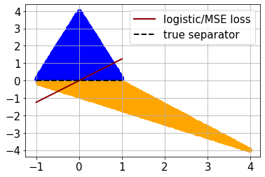
Figure 4: Blue points show samples from the positive distribution and orange points show samples from the negative distribution. Unalabeled data is obtained by mixing positive and negative distribution with equal proportion. BCE (or Brier) loss minimization on P vs U data leads to a classifiers that is not consistent with the ranking of the Bayes optimal score function.

Now we show that under the subdomain assumption [39, 35], any monotonic transformation of Bayes optimal scoring function induces positive pure bin property. First, we define the subdomain assumption.

Assumption 1 (Subdomain assumption).

A family of subsets $\mathcal{S}\subseteq 2^{\mathcal{X}}$, and distributions $p_{p}$, $p_{n}$ are said to satisfy the anchor set condition with margin $\gamma>0$, if there exists a compact set $A\in\mathcal{S}$ such that $A\subseteq\text{supp}(p_{p})/\text{supp}(p_{n})$ and $p_{p}(A)\geq\gamma$.

Note that any monotonic mapping of the Bayes optimal scoring function can be represented by $\tau^{\prime}=g\circ\tau$, where g is a monotonic function and

$$\tau(x)=\begin{cases}p_{p}(x)/p_{u}(x)\quad&\text{if }p_{p}(x)>0\\ 0\quad&\text{o.w}\,.\end{cases}$$ (31)

For any point $x\in A$ and $x^{\prime}\in\mathcal{X}/A$, we have $\tau(x)>\tau(x^{\prime})$ which implies $\tau^{\prime}(x)>\tau^{\prime}(x^{\prime})$. Thus, any monotonic mapping of Bayes optimal scoring function yields the positive pure bin property with $\epsilon_{p}\geq\gamma$.

Appendix E Analysis of CVIR

First we analyse our loss function in the scenario when the support of positives and negatives is separable. We assume that the true alpha $\alpha$ is known and we have access to populations of positive and unlabeled data. We also assume that their exists a separator $f^{*}:\mathcal{X}\mapsto\{0,1\}$ that can perfectly separate the positive and negative distribution, i.e., $\int dxp_{p}(x)\mathbb{I}\left[f^{*}(x)\neq 1\right]+\int dxp_{n}(x)\mathbb{I}\left[f^{*}(x)\neq 0\right]=0$. Our learning objective can be written as jointly optimizing a classifier $f$ and a weighting function $w$ on the unlabeled distribution:

$$\min_{f\in\mathcal{F},w}\int dxp_{p}(x)l(f(x),1)+\frac{1}{1-\alpha}\int dxp_{u}(x)w(x)l(f(x),0)\,,$$

$$\text{ s.t. }w:\mathcal{X}\mapsto[0,1]\,,\int dxp_{u}(x)w(x)=1-\alpha\,.$$ (32)

The following proposition shows that minimizing the objective (32) on separable positive and negative distributions gives a perfect classifier.

Proposition 1.

For $\alpha\in(0,1)$, if there exists a classifier $f^{*}\in\mathcal{F}$ that can perfectly separate the positive and negative distributions, optimizing objective (32) with 0-1 loss leads to a classifier $f$ that achieves $0$ classification error on the unlabeled distribution.

Proof.

First we observe that having $w(x)=1-f^{*}(x)$ leads to the objective value being minimized to 0 as well as a perfect classifier $f$. This is because

$$\frac{1}{1-\alpha}\int dxp_{u}(x)(1-f^{*}(x))l(f(x),0)=\int dxp_{n}(x)l(f(x),0)$$

thus the objective becomes classifying positive v.s. negative, which leads to a perfect classifier if $\mathcal{F}$ contains one. Now we show that for any $f$ such that the classification error is non-zero then the objective (32) must be greater than zero no matter what $w$ is. Suppose $f$ satisfies

$$\int dxp_{p}(x)l(f(x),1)+\int dxp_{n}(x)l(f(x),0)>0\,.$$

We know that either $\int dxp_{p}(x)l(f(x),1)>0$ or $\int dxp_{n}(x)l(f(x),0)>0$ will hold. If $\int dxp_{p}(x)l(f(x),1)>0$ we know that (32) must be positive. If $\int dxp_{p}(x)l(f(x),1)=0$ and $\int dxp_{n}(x)l(f(x),0)>0$ we have $l(f(x),0)=1$ almost everywhere in $p_{p}(x)$ thus

$$\frac{1}{1-\alpha}\int dxp_{u}(x)w(x)l(f(x),0)$$

$$=\frac{\alpha}{1-\alpha}\int dxp_{p}(x)w(x)l(f(x),0)+\int dxp_{n}(x)w(x)l(f(x),0)$$

$$=\frac{\alpha}{1-\alpha}\int dxp_{p}(x)w(x)+\int dxp_{n}(x)w(x)l(f(x),0)\,.$$

If $\int dxp_{p}(x)w(x)>0$ we know that (32) must be positive. If $\int dxp_{p}(x)w(x)=0$, since we know that

$$\int dxp_{u}(x)w(x)=\alpha\int dxp_{p}(x)w(x)+(1-\alpha)\int dxp_{n}(x)w(x)=1-\alpha$$

we have $\int dxp_{n}(x)w(x)=1$ which means $w(x)=1$ almost everywhere in $p_{n}(x)$. This leads to the fact that $\int dxp_{n}(x)l(f(x),0)>0$ indicates $\int dxp_{n}(x)w(x)l(f(x),0)>0$, which concludes the proof.

∎

The intuition is that, any classifier that discards an $\widetilde{\alpha}>0$ proportion of negative distribution from unlabeled will have loss strictly greater than zero with our CVIR objective. Since only a perfect linear separator (with weights $\to\infty$) can achieves loss $\to 0$, CVIR objective will (correctly) discard the $\alpha$ proportion of positive from unlabeled data achieving a classifier that perfectly separates the data.

We leave theoretic investigation on non-separable distributions for future work. However, as an initial step towards a general theory, we show that in the population case one step of our alternating procedure cannot increase the loss.

Consider the following objective function

$$L(f_{t},w_{t}) =E_{x\sim P_{p}}[l(f_{t}(x),0)]+E_{x\sim P_{u}}[w_{t}(x)l(f_{t}(x),1)]$$ (33)

such that $$E_{x\sim P_{u}}[w(x)]=1-\alpha\text{ and }w(x)\in\{0,1\}$$

Given $f_{t}$ and $w_{t}$, CVIR can be summarized as the following two step iterative procedure: (i) Fix $f_{t}$, optimize the loss to obtain $w_{t+1}$; and (ii) Fix $w_{t+1}$ and optimize the loss to obtain $f_{t+1}$. By construction of CVIR, we select $w_{t+1}$ such that we discard points with highest loss, and hence $L(f_{t},w_{t+1})\leq L(f_{t},w_{t})$. Fixing $w_{t+1}$, we minimize the $L(f_{t},w_{t+1})$ to obtain $f_{t+1}$ and hence $L(f_{t+1},w_{t+1})\leq L(f_{t},w_{t+1})$. Combining these two steps, we get $L(f_{t+1},w_{t+1})\leq L(f_{t},w_{t})$.

Appendix F Experimental Details

Below we present dataset details. We present experiments with MNIST Overlap in App. G.8.

Dataset	Simulated PU Dataset	P vs N	#Positives		#Unlabeled
			Train	Val	Train	Val
CIFAR10	Binarized CIFAR	[0-4] vs [5-9]	12500	12500	2500	2500
	CIFAR Dog vs Cat	3 vs 5	2500	2500	500	500
MNIST	Binarized MNIST	[0-4] vs [5-9]	15000	15000	2500	2500
	MNIST 17	1 vs 7	3000	3000	500	500
	MNIST Overlap	[0-7] vs [3-9]	150000	15000	2500	2500
IMDb	IMDb	pos vs neg	6250	6250	5000	5000

For CIFAR dataset, we also use the standard data augementation of random crop and horizontal flip. PyTorch code is as follows:

(transforms.RandomCrop(32, padding=4),
transforms.RandomHorizontalFlip())

F.1 Architecture and Implementation Details

All experiments were run on NVIDIA GeForce RTX 2080 Ti GPUs. We used PyTorch [33] and Keras with Tensorflow [1] backend for experiments.

For CIFAR10, we experiment with convolutional nets and MLP. For MNIST, we train MLP. In particular, we use ResNet18 [19] and all convolution net [40] . Implementation adapted from: https://github.com/kuangliu/pytorch-cifar.git. We consider a 4-layered MLP. The PyTorch code for 4-layer MLP is as follows:

nn.Sequential(nn.Flatten(),
nn.Linear(input_dim, 5000, bias=True),
nn.ReLU(),
nn.Linear(5000, 5000, bias=True),
nn.ReLU(),
nn.Linear(5000, 50, bias=True),
nn.ReLU(),
nn.Linear(50, 2, bias=True)
)

For all architectures above, we use Xaviers initialization [18]. For all methods except nnPU and uPU, we do cross entropy loss minimization with SGD optimizer with momentum $0.9$. For convolution architectures we use a learning rate of $0.1$ and MLP architectures we use a learning rate of $0.05$. For nnPU and uPU, we minimize sigmoid loss with ADAM optimizer with learning rate $0.0001$ as advised in its original paper. For all methods, we fix the weight decay param at $0.0005$.

For IMDb dataset, we fine-tune an off-the-shelf uncased BERT model [10]. Code adapted from Hugging Face Transformers [42]: https://huggingface.co/transformers/v3.1.0/custom_datasets.html. For all methods except nnPU and uPU, we do cross entropy loss minimization with Adam optimizer with learning rate $0.00005$ (default params). With the same hyperparameters and Sigmoid loss, we could not train BERT with nnPU and uPU due to vanishing gradients. Instead we use learning rate $0.00001$.

F.2 Division between training set and hold-out set

Since the training set is used to learn the classifier (parameters of a deep neural network) and the hold-out set is just used to learn the mixture proportion estimate (scalar), we use a larger dataset for training. Throughout the experiments, we use an 80-20 split of the original set.

At a high level, we have an error bound on the mixture proportion estimate and we can use that to decide the split in general. As long as we use enough samples to make the $\mathcal{O}(1/\sqrt{n})$ small in our bound in Theorem 1, we can use the rest of the samples to learn the classifier.

Appendix G Additional Experiments

G.1 nnPU vs PN classification

In this section, we compare the performance of nnPU and PvN training on the same positive and negative (from the unlabeled) data at $\alpha=0.5$. We highlight the huge classification performance gap between nnPU and PvN training and show that training with CVuO objective partially recovers the performance gap. Note, to train PvN classifier, we use the same hyperparameters as that with PvU training.

Dataset	Model	nnPU (known $\alpha$)	PvN	CVuO (known $\alpha$)	(TED)n (unknown $\alpha$)
Binarized CIFAR	ResNet	$76.8$	$86.9$	$82.6$	$82.7$
	All Conv	$72.1$	$76.7$	$77.1$	$76.8$
	MLP	$63.9$	$65.1$	$65.9$	$63.2$
CIFAR Dog vs Cat	ResNet	$72.6$	$80.4$	$74.0$	$76.1$
	All Conv	$68.4$	$77.9$	$71.0$	$72.2$
Binarized MNIST	MLP	$95.9$	$96.7$	$96.4$	$95.9$
MNIST17	MLP	$98.2$	$99.0$	$98.6$	$98.6$
IMDb	BERT	$86.2$	$89.1$	$87.4$	$88.1$

Table 4: Accuracy for PvN classification with nnPU, PvN, CVuO objective and (TED)ⁿ training. Results reported by aggregating aggregating over 10 epochs.

G.2 Under-Fitting due to pessimistic early stopping

Ivanov [20] explored the following heuristics for ad-hoc early stopping criteria: training proceeds until the loss on unseen PU data ceases to decrease. In particular, the authors suggested early stopping criterion based on the loss on unseen PU data doesn’t decrease in epochs separated by a pre-defined window of length $l$. The early stopping is done when this happens consecutively for $l$ epochs. However, this approach leads to severe under-fitting. When we fix $l=5$, we observe a significant performance drop in CIFAR classification and MPE.

With PvU training, the performance of ResNet model on Binarized CIFAR (in Table 2) drops from $78.3$ (orcale stopping) to $60.4$ (with early stopping). Similar on CIFAR CAT vs Dog, the performance of the same architecture drops from $71.6$ (orcale stopping) to $58.4$ (with early stopping). Note that the decrease in accuracy is less or not significant for MNIST. With PvU training, the performance of MLP model on Binarized MNIST (in Table 2) drops from $94.5$ (orcale stopping) to $94.1$ (with early stopping). This is because we obtain good performance on MNIST early in training.

G.3 Results parallel to Fig. 3

Epoch wise results for all models for Binarized CIFAR, CIFAR Dog vs Cat, Binarized MNIST, MNIST 17 and IMDb.

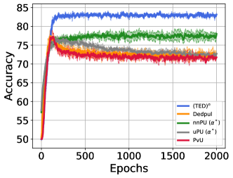
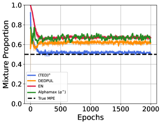
Figure 5: Epoch wise results with ResNet-18 network trained on CIFAR-binarized.

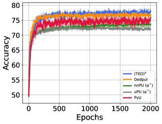
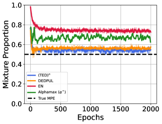
Figure 6: Epoch wise results with All convolutional network trained on CIFAR-binarized.

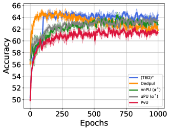
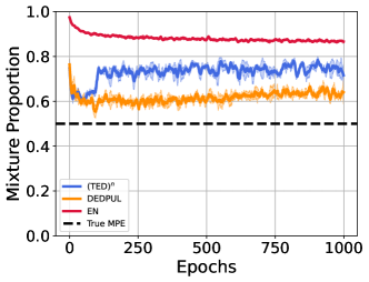
Figure 7: Epoch wise results with FCN trained on CIFAR-binarized.

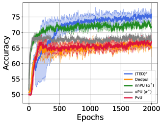
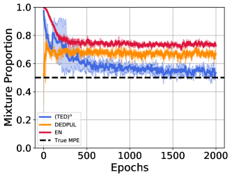
Figure 8: Epoch wise results with ResNet-18 trained on CIFAR Dog vs Cat.

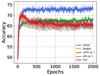
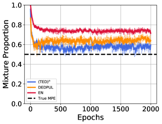
Figure 9: Epoch wise results with All convolutional network trained on CIFAR Dog vs Cat.

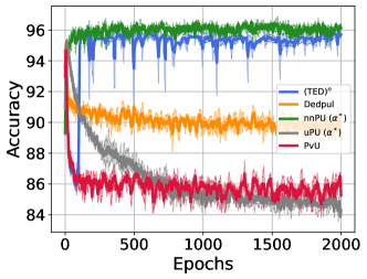
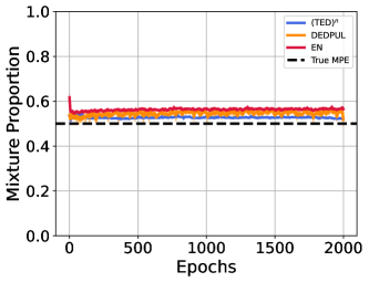
Figure 10: Epoch wise results with MLP trained on Binarized MNIST.

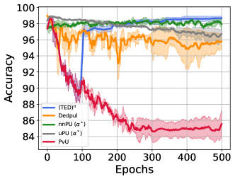
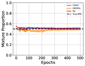
Figure 11: Epoch wise results with MLP trained on MNIST 17.

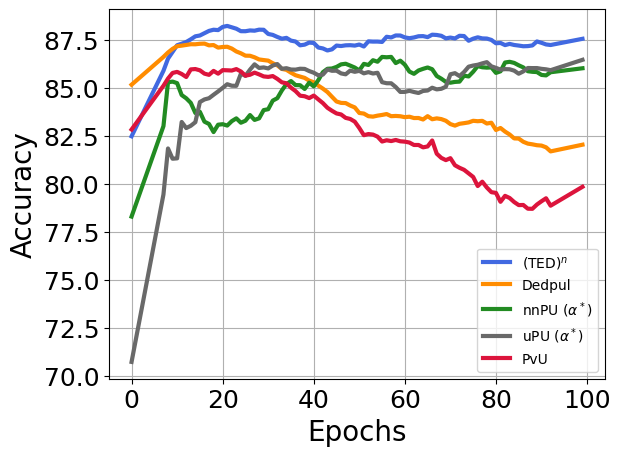
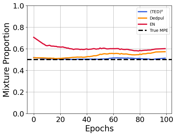
Figure 12: Epoch wise results with BERT trained on IMDb.

G.4 Overfitting on unlabeled data as PvU training proceeds

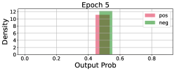
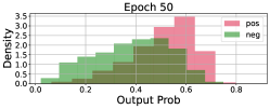
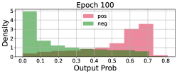
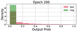
Figure 13: Score assigned by the classifier to positive and negative points in the unlabeled training set as PvU training proceeds. As training proceeds, classifier memorizes both positive and negative in unlabeled as negatives.

In Fig. 13, we show the distribution of unlabeled training points. We show that as positive versus unlabeled training proceeds with a ResNet-18 model on binarized CIFAR dataset, classifier memorizes all the unlabeled data as negative assigning them very small scores (i.e., the probability of them being negative).

G.5 Ablations to (TED)ⁿ

Varying the number of warm start epochs We now vary the number of warm start epochs with (TED)ⁿ. We observe that increasing the number of warm start epochs doesn’t hurt (TED)ⁿ even when the classifier at the end of the warm start training memorized PU training data due PvU training. While in many cases (TED)ⁿ training without warm start is able to recover the same performance, it fails to learn anything for CIFAR Dog vs Cat with all convolutional neural network. This highlights the need for warm start training with (TED)ⁿ.

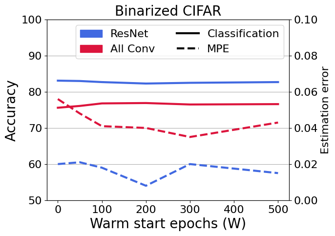
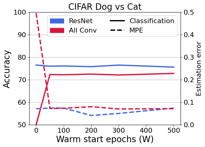
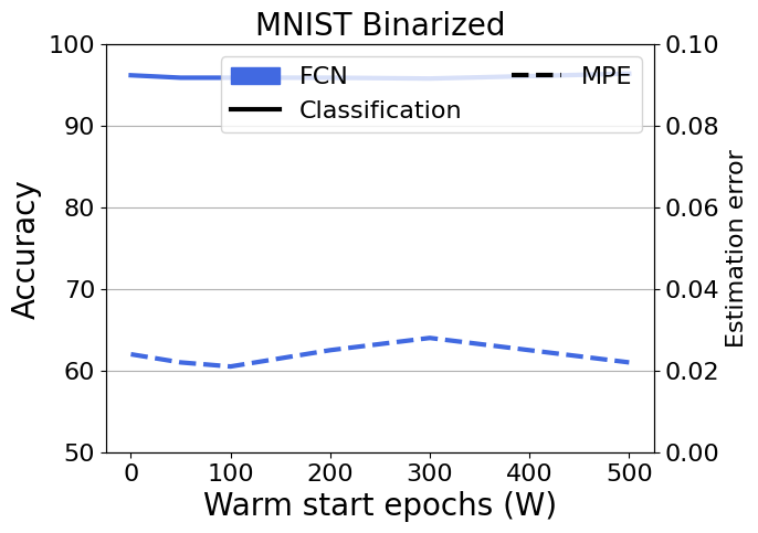
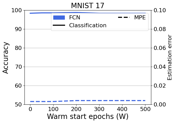
Figure 14: Classification and MPE results with varying warm start epochs $W$ with (TED)ⁿ

Varying the true mixture proportion $\alpha$ Next, we vary $\alpha$, the true mixture proportion and present results for MPE and classification in Fig. 15. Overall, across all $\alpha$, our method (TED)ⁿ is able to achieve superior performance as compared to alternate algorithms. We omit high $\alpha$ for CIFAR and IMDb datasets as all the methods result in trivial accuracy and mixture proportion estimate.

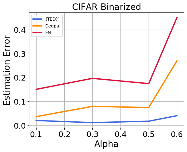
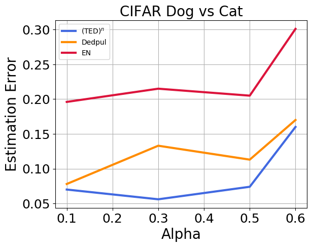
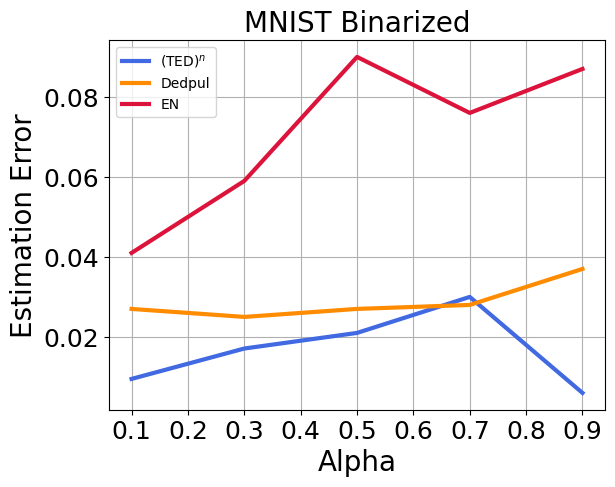
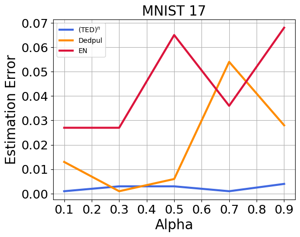
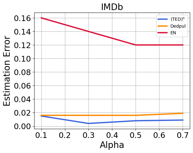
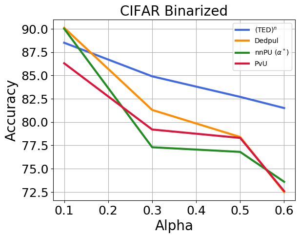
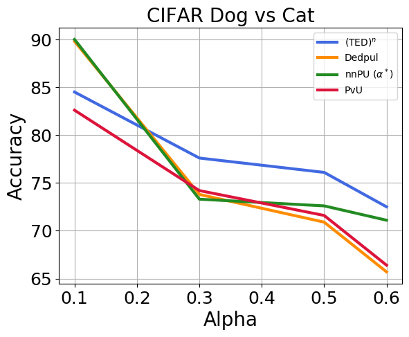
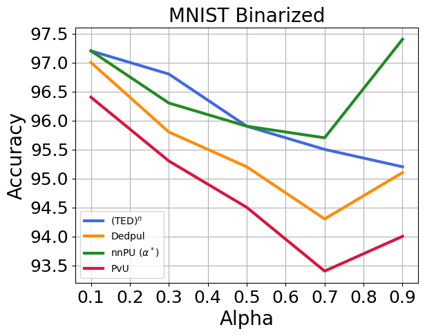
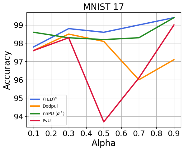
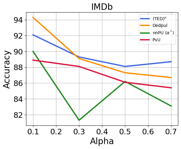
Figure 15: MPE and Classification results with varying mixture proportion. For each method we show results with the best performing architecture.

G.6 Classification and MPE results with error bars

Dataset Model (TED)ⁿ BBE^∗ DEDPUL^∗ EN KM2 TiCE Binarized CIFAR ResNet $\mathbf{0.026\pm 0.005}$ $0.091\pm 0.027$ $0.091\pm 0.023$ $0.192\pm 0.007$ All Conv $0.042\pm 0.003$ $\mathbf{0.037\pm 0.018}$ $0.052\pm 0.017$ $0.221\pm 0.017$ $0.168\pm 0.207$ $0.194\pm 0.039$ MLP $0.225\pm 0.013$ $0.177\pm 0.011$ $\mathbf{0.138\pm 0.009}$ $0.372\pm 0.002$ CIFAR Dog vs Cat ResNet $\mathbf{0.078\pm 0.010}$ $0.176\pm 0.015$ $0.170\pm 0.010$ $0.226\pm 0.003$ $0.331\pm 0.238$ $0.286\pm 0.013$ All Conv $\mathbf{0.066\pm 0.015}$ $0.128\pm 0.020$ $0.115\pm 0.014$ $0.250\pm 0.019$ Binarized MNIST MLP $\mathbf{0.024\pm 0.001}$ $0.032\pm 0.001$ $0.031\pm 0.003$ $0.080\pm 0.009$ $0.029\pm 0.008$ $0.056\pm 0.05$ MNIST17 MLP $\mathbf{0.003\pm 0.000}$ $0.023\pm 0.017$ $0.021\pm 0.011$ $0.028\pm 0.017$ $0.022\pm 0.003$ $0.043\pm 0.023$ IMDb BERT $\mathbf{0.008\pm 0.001}$ $0.011\pm 0.002$ $0.016\pm 0.005$ $0.07\pm 0.01$ - -

Table 5: Absolute estimation error when $\alpha$ is 0.5. "*" denote oracle early stopping as defined in Sec. 6. Results reported by aggregating absolute error over 10 epochs and 3 seeds.

Dataset Model (TED)ⁿ (unknown $\alpha$) CVIR (known $\alpha$) PvU^∗ (known $\alpha$) DEDPUL^∗ (unknown $\alpha$) nnPU (known $\alpha$) uPU^∗ (known $\alpha$) Binarized CIFAR ResNet $\mathbf{82.7\pm 0.13}$ $82.3\pm 0.18$ $76.9\pm 1.12$ $77.1\pm 1.52$ $77.2\pm 1.03$ $76.7\pm 0.74$ All Conv $77.9\pm 0.29$ $\mathbf{78.1\pm 0.47}$ $75.8\pm 0.75$ $77.1\pm 0.64$ $73.4\pm 1.31$ $72.5\pm 0.21$ MLP $64.2\pm 0.37$ $\mathbf{66.9\pm 0.28}$ $61.6\pm 0.38$ $62.6\pm 0.30$ $63.1\pm 0.79$ $64.0\pm 0.24$ CIFAR Dog vs Cat ResNet $\mathbf{75.2\pm 1.74}$ $73.3\pm 0.94$ $67.3\pm 1.52$ $67.0\pm 1.46$ $71.8\pm 0.33$ $68.8\pm 0.53$ All Conv $\mathbf{73.0\pm 0.81}$ $71.7\pm 0.47$ $70.5\pm 0.60$ $69.2\pm 0.86$ $67.9\pm 0.52$ $67.5\pm 2.28$ Binarized MNIST MLP $95.6\pm 0.42$ $\mathbf{96.3\pm 0.07}$ $94.2\pm 0.58$ $94.8\pm 0.10$ $96.1\pm 0.14$ $95.2\pm 0.19$ MNIST17 MLP $\mathbf{98.7\pm 0.25}$ $\mathbf{98.7\pm 0.09}$ $96.9\pm 1.51$ $97.7\pm 0.62$ $98.4\pm 0.20$ $98.4\pm 0.09$ IMDb BERT $\mathbf{87.6\pm 0.20}$ $87.4\pm 0.25$ $86.1\pm 0.53$ $87.3\pm 0.18$ $86.2\pm 0.25$ $85.9\pm 0.12$

Table 6: Accuracy for PvN classification with PU learning. "*" denote oracle early stopping as defined in Sec. 6. Results reported by aggregating over 10 epochs and 3 seeds.

G.7 Experiments on UCI dataset

In this section, we will present results on 5 UCI datasets.

Dataset	#Positives		#Unlabeled
	Train	Val	Train	Val
concrete	162	162	81	81
mushroom	1304	1304	652	652
landsat	946	946	472	472
pageblock	185	185	92	92
spambase	604	604	302	302

We train a MLP with 2 hidden layers each with $512$ units. The PyTorch code for 4-layer MLP is as follows:

nn.Sequential(nn.Flatten(),
nn.Linear(input_dim, 512, bias=True),
nn.ReLU(),
nn.Linear(512, 512, bias=True),
nn.ReLU(),
nn.Linear(512, 2, bias=True),
)

Similar to vision datasets and architectures, we do cross entropy loss minimization with SGD optimizer with momentum $0.9$ and learning rate $0.1$. For nnPU and uPU, we minimize sigmoid loss with ADAM optimizer with learning rate $0.0001$ as advised in its original paper. For all methods, we fix the weight decay param at $0.0005$.

Dataset	(TED)n	BBE∗	DEDPUL∗	EN∗	KM2	TiCE
concrete	$\mathbf{0.071}$	$0.152$	$0.176$	$0.239$	$0.099$	$0.268$
mushroom	$\mathbf{0.001}$	$0.015$	$0.014$	$0.013$	$0.038$	$0.069$
landsat	${0.022}$	$0.021$	$\mathbf{0.012}$	$0.080$	$0.037$	$0.027$
pageblock	$\mathbf{0.007}$	$0.066$	$0.041$	$0.135$	$0.008$	$0.298$
spambase	$\mathbf{0.006}$	$0.047$	$0.077$	$0.127$	$0.062$	$0.276$

Table 7: Absolute estimation error when $\alpha$ is 0.5. "*" denote oracle early stopping as defined in Sec. 6. Results reported by aggregating absolute error over 10 epochs.

Dataset	(TED)n (unknown $\alpha$)	CVuO (known $\alpha$)	PvU∗ (known $\alpha$)	DEDPUL∗ (unknown $\alpha$)	nnPU (known $\alpha$)	uPU∗ (known $\alpha$)
concrete	$\mathbf{86.3}$	$80.1$	$83.1$	$83.7$	$83.2$	$84.4$
mushroom	$96.4$	$96.3$	$\mathbf{98.7}$	$\mathbf{98.7}$	$97.5$	$93.9$
landsat	$\mathbf{93.8}$	$93.1$	$93.4$	$92.4$	$92.9$	$92.3$
pageblock	$\mathbf{95.7}$	$\mathbf{95.7}$	$95.1$	$94.5$	$93.9$	$93.9$
spambase	$\mathbf{89.4}$	$88.1$	$89.2$	$86.8$	$88.5$	$87.7$

Table 8: Accuracy for PvN classification with PU learning. "*" denote oracle early stopping as defined in Sec. 6. Results reported by aggregating aggregating over 10 epochs.

On $4$ out of $5$ UCI datasets, our proposed methods are better than the best performing alternatives (Table 7 and Table 8).

G.8 Experiments on MNIST Overlap

Similar to binarized MNIST, we create a new dataset called MNIST Overlap, where the positive class contains digits from $0$ to $7$ and the negative class contains digits from $3$ to $9$. This creates a dataset with overlap between positive and negative support. Note that while the supports overlap, we sample images from the overlap classes with replacement, and hence, in absence of duplicates in the dataset, exact same images don’t appear both in positive and negative subsets.

We train MLP with the same hyperparameters as before. Our findings in Table 9 and Table 10 highlight superior performance of the proposed approaches in the cases of support overlap.

Dataset	(TED)n	BBE∗	DEDPUL∗	EN∗	KM2	TiCE
MNIST Overlap	$\mathbf{0.035}$	$0.100$	$0.104$	$0.196$	$0.099$	$0.074$

Table 9: Absolute estimation error when $\alpha$ is 0.5. "*" denote oracle early stopping as defined in Sec. 6. Results reported by aggregating absolute error over 10 epochs.

Dataset	(TED)n (unknown $\alpha$)	CVuO (known $\alpha$)	PvU∗ (known $\alpha$)	DEDPUL∗ (unknown $\alpha$)	nnPU (known $\alpha$)	uPU∗ (known $\alpha$)
MNIST Overlap	$\mathbf{79.0}$	$78.4$	$77.4$	$77.5$	$78.6$	$78.8$

Table 10: Accuracy for PvN classification with PU learning. "*" denote oracle early stopping as defined in Sec. 6. Results reported by aggregating aggregating over 10 epochs.

References

- Abadi et al. [2016] M. Abadi, P. Barham, J. Chen, Z. Chen, A. Davis, J. Dean, M. Devin, S. Ghemawat, G. Irving, M. Isard, et al. Tensorflow: A system for large-scale machine learning. In 12th USENIX Symposium on Operating Systems Design and Implementation, 2016.
- Alexandari et al. [2019] A. Alexandari, A. Kundaje, and A. Shrikumar. Adapting to label shift with bias-corrected calibration. In arXiv preprint arXiv:1901.06852, 2019.
- Azizzadenesheli et al. [2019] K. Azizzadenesheli, A. Liu, F. Yang, and A. Anandkumar. Regularized learning for domain adaptation under label shifts. In International Conference on Learning Representations (ICLR), 2019.
- Bekker and Davis [2018] J. Bekker and J. Davis. Estimating the class prior in positive and unlabeled data through decision tree induction. In Proceedings of the AAAI Conference on Artificial Intelligence, 2018.
- Bekker and Davis [2020] J. Bekker and J. Davis. Learning from positive and unlabeled data: a survey. Mach. Learn., 2020.
- Blanchard et al. [2010] G. Blanchard, G. Lee, and C. Scott. Semi-supervised novelty detection. The Journal of Machine Learning Research, 11:2973–3009, 2010.
- Byrd and Lipton [2019] J. Byrd and Z. C. Lipton. What is the effect of importance weighting in deep learning? In International Conference on Machine Learning (ICML), 2019.
- De Comité et al. [1999] F. De Comité, F. Denis, R. Gilleron, and F. Letouzey. Positive and unlabeled examples help learning. In International Conference on Algorithmic Learning Theory, pages 219–230. Springer, 1999.
- Denis [1998] F. Denis. Pac learning from positive statistical queries. In International Conference on Algorithmic Learning Theory, pages 112–126. Springer, 1998.
- Devlin et al. [2018] J. Devlin, M.-W. Chang, K. Lee, and K. Toutanova. Bert: Pre-training of deep bidirectional transformers for language understanding. arXiv preprint arXiv:1810.04805, 2018.
- Du Plessis et al. [2015] M. Du Plessis, G. Niu, and M. Sugiyama. Convex formulation for learning from positive and unlabeled data. In International conference on machine learning, pages 1386–1394, 2015.
- Du Plessis and Sugiyama [2014a] M. C. Du Plessis and M. Sugiyama. Class prior estimation from positive and unlabeled data. IEICE TRANSACTIONS on Information and Systems, 97(5):1358–1362, 2014a.
- Du Plessis and Sugiyama [2014b] M. C. Du Plessis and M. Sugiyama. Semi-supervised learning of class balance under class-prior change by distribution matching. Neural Networks, 50:110–119, 2014b.
- Du Plessis et al. [2014] M. C. Du Plessis, G. Niu, and M. Sugiyama. Analysis of learning from positive and unlabeled data. Advances in neural information processing systems, 27:703–711, 2014.
- Dvoretzky et al. [1956] A. Dvoretzky, J. Kiefer, and J. Wolfowitz. Asymptotic minimax character of the sample distribution function and of the classical multinomial estimator. The Annals of Mathematical Statistics, pages 642–669, 1956.
- Elkan and Noto [2008] C. Elkan and K. Noto. Learning classifiers from only positive and unlabeled data. In Proceedings of the 14th ACM SIGKDD international conference on Knowledge discovery and data mining, pages 213–220, 2008.
- Garg et al. [2020] S. Garg, Y. Wu, S. Balakrishnan, and Z. C. Lipton. A unified view of label shift estimation. arXiv preprint arXiv:2003.07554, 2020.
- Glorot and Bengio [2010] X. Glorot and Y. Bengio. Understanding the difficulty of training deep feedforward neural networks. In Proceedings of the thirteenth international conference on artificial intelligence and statistics, pages 249–256. JMLR Workshop and Conference Proceedings, 2010.
- He et al. [2016] K. He, X. Zhang, S. Ren, and J. Sun. Deep Residual Learning for Image Recognition. In Computer Vision and Pattern Recognition (CVPR), 2016.
- Ivanov [2019] D. Ivanov. DEDPUL: Difference-of-estimated-densities-based positive-unlabeled learning. arXiv preprint arXiv:1902.06965, 2019.
- Jain et al. [2016] S. Jain, M. White, M. W. Trosset, and P. Radivojac. Nonparametric semi-supervised learning of class proportions. arXiv preprint arXiv:1601.01944, 2016.
- Kingma and Ba [2014] D. P. Kingma and J. Ba. Adam: A Method for Stochastic Optimization. arXiv Preprint arXiv:1412.6980, 2014.
- Kiryo et al. [2017] R. Kiryo, G. Niu, M. C. Du Plessis, and M. Sugiyama. Positive-unlabeled learning with non-negative risk estimator. In Advances in neural information processing systems, pages 1675–1685, 2017.
- Krizhevsky and Hinton [2009] A. Krizhevsky and G. Hinton. Learning Multiple Layers of Features from Tiny Images. Technical report, Citeseer, 2009.
- LeCun et al. [1998] Y. LeCun, L. Bottou, Y. Bengio, and P. Haffner. Gradient-Based Learning Applied to Document Recognition. Proceedings of the IEEE, 86, 1998.
- Lee and Liu [2003] W. S. Lee and B. Liu. Learning with positive and unlabeled examples using weighted logistic regression. In ICML, volume 3, pages 448–455, 2003.
- Letouzey et al. [2000] F. Letouzey, F. Denis, and R. Gilleron. Learning from positive and unlabeled examples. In International Conference on Algorithmic Learning Theory, pages 71–85. Springer, 2000.
- Li and Liu [2003] X. Li and B. Liu. Learning to classify texts using positive and unlabeled data. In IJCAI. Citeseer, 2003.
- Lipton et al. [2018] Z. C. Lipton, Y.-X. Wang, and A. Smola. Detecting and Correcting for Label Shift with Black Box Predictors. In International Conference on Machine Learning (ICML), 2018.
- Liu et al. [2002] B. Liu, W. S. Lee, P. S. Yu, and X. Li. Partially supervised classification of text documents. In ICML, 2002.
- Liu et al. [2003] B. Liu, Y. Dai, X. Li, W. S. Lee, and P. S. Yu. Building text classifiers using positive and unlabeled examples. In Third IEEE International Conference on Data Mining, pages 179–186. IEEE, 2003.
- Maas et al. [2011] A. Maas, R. E. Daly, P. T. Pham, D. Huang, A. Y. Ng, and C. Potts. Learning word vectors for sentiment analysis. In Proceedings of the 49th annual meeting of the association for computational linguistics: Human language technologies, pages 142–150, 2011.
- Paszke et al. [2019] A. Paszke, S. Gross, F. Massa, A. Lerer, J. Bradbury, G. Chanan, T. Killeen, Z. Lin, N. Gimelshein, L. Antiga, A. Desmaison, A. Kopf, E. Yang, Z. DeVito, M. Raison, A. Tejani, S. Chilamkurthy, B. Steiner, L. Fang, J. Bai, and S. Chintala. Pytorch: An imperative style, high-performance deep learning library. In Advances in Neural Information Processing Systems 32, 2019.
- Rabanser et al. [2019] S. Rabanser, S. Günnemann, and Z. C. Lipton. Failing loudly: An empirical study of methods for detecting dataset shift. In Advances in Neural Information Processing Systems (NeurIPS), 2019.
- Ramaswamy et al. [2016] H. Ramaswamy, C. Scott, and A. Tewari. Mixture proportion estimation via kernel embeddings of distributions. In International conference on machine learning, pages 2052–2060, 2016.
- Reeve and Kabán [2019] H. Reeve and A. Kabán. Exploiting geometric structure in mixture proportion estimation with generalised blanchard-lee-scott estimators. In Proceedings of the 30th International Conference on Algorithmic Learning Theory, pages 682–699. PMLR, 2019.
- Saerens et al. [2002] M. Saerens, P. Latinne, and C. Decaestecker. Adjusting the Outputs of a Classifier to New a Priori Probabilities: A Simple Procedure. Neural Computation, 2002.
- Sanderson and Scott [2014] T. Sanderson and C. Scott. Class proportion estimation with application to multiclass anomaly rejection. In Artificial Intelligence and Statistics, pages 850–858, 2014.
- Scott [2015] C. Scott. A rate of convergence for mixture proportion estimation, with application to learning from noisy labels. In Artificial Intelligence and Statistics, pages 838–846, 2015.
- Springenberg et al. [2014] J. T. Springenberg, A. Dosovitskiy, T. Brox, and M. Riedmiller. Striving for simplicity: The all convolutional net. arXiv preprint arXiv:1412.6806, 2014.
- Storkey [2009] A. Storkey. When Training and Test Sets Are Different: Characterizing Learning Transfer. Dataset Shift in Machine Learning, 2009.
- Wolf et al. [2020] T. Wolf, L. Debut, V. Sanh, J. Chaumond, C. Delangue, A. Moi, P. Cistac, T. Rault, R. Louf, M. Funtowicz, J. Davison, S. Shleifer, P. von Platen, C. Ma, Y. Jernite, J. Plu, C. Xu, T. L. Scao, S. Gugger, M. Drame, Q. Lhoest, and A. M. Rush. Transformers: State-of-the-art natural language processing. In Proceedings of the 2020 Conference on Empirical Methods in Natural Language Processing: System Demonstrations, pages 38–45. Association for Computational Linguistics, 2020.
- Zhang et al. [2016] C. Zhang, S. Bengio, M. Hardt, B. Recht, and O. Vinyals. Understanding deep learning requires rethinking generalization. arXiv preprint arXiv:1611.03530, 2016.
- Zhang and Lee [2005] D. Zhang and W. S. Lee. A simple probabilistic approach to learning from positive and unlabeled examples. In Proceedings of the 5th annual UK workshop on computational intelligence (UKCI), pages 83–87, 2005.