Nonparametric Cointegrating Regression Functions with Endogeneity and Semi-Long Memory

Abstract

This article develops nonparametric cointegrating regression models with endogeneity and semi-long memory. We assume semi-long memory is produced in the regressor process by tempering of random shock coefficients. The fundamental properties of long memory processes are thus retained in the regressor process. Nonparametric nonlinear cointegrating regressions with serially dependent errors and endogenous regressors that are driven by long memory innovations have been considered in Wang and Phillips (2016). That work also implemented a statistical specification test for testing whether the regression function follows a parametric form. The convergence rate of the proposed test is parameter dependent, and its limit theory involves the local time of fractional Brownian motion. The present paper modifies the test statistic proposed for the long memory case by Wang and Phillips (2016) to be suitable for the semi-long memory case. With this modification, the limit theory for the test involves the local time of standard Brownian motion. Through simulation studies, we investigate properties of nonparametric regression function estimation with semi-long memory regressors as well as long memory regressors.

Keywords: Fractional differencing parameter; test statistic; standard Brownian motion; simulation studies; tempered process.

Introduction

Regression models that relate two time series have long been of interest in economics, and any number of quantities of interest in such models are nonstationary. If two variables in a linear regression model are integrated (in the time series sense) of the same order, but some linear combinations of them are stationary then the model is said to be a cointegrated regression model. That label is also used to refer to models in which the covariate or regressor process is nonstationary and the response process is related to it through a nonlinear function (see Tjøstheim (2020) for a recent review). Nonlinear cointegrated regression models have been applied to, among others, problems in financial markets, stock prices, heavy traffic, and energy markets (e.g., Fasen (2013) and references therein). In particular, let

$$y_{k}=f(x_{k})+u_{k},\qquad k=1,\ldots,N,$$ (1)

be a nonlinear cointegrating regression model, where $x_{k}$ is a nonstationary regressor, $u_{k}$ is an error process, and $f(\cdot)$ is an unknown real function.

Two problems that have been the focus of much research are estimation of the unknown regression function $f(\cdot)$ nonparametrically, and testing that $f(\cdot)$ has a particular parametric form. Many of the theoretical results related to these problems have assumed strict exogeneity in which the regressor $x_{k}$ is assumed to be uncorrelated with the regression error $u_{k}$ (e.g., Karlsen et al. (2007), Cai et al. (2009), Wang and Phillips (2009a), and Wang (2014)). Often, the regressor $x_{k}$ is assumed to be a short memory process. Extending this framework by allowing the regressor $x_{k}$ to be driven by long memory innovations and permitting correlation with $u_{k}$ (so-called endogeneity) has received less attention in the literature and leads to some technical problems that have not been completely resolved.

Recently, Wang and Phillips (2016) established a limit theory for nonparametric estimation of regression models that allow for both endogeneity and long memory in the regressor process. They also developed a test statistic for parametric forms of regression functions of the type $f(x)=g(x,\theta_{0})$ where $g(\cdot,\theta_{0})$ represents a parametric family of functions with unknown parameter $\theta_{0}\in\Theta$. The authors assumed that $\Theta$ is a compact subspace of $\mathbb{R}^{m}$ for some finite $m$. The test of Wang and Phillips (2016) is a modification of a test statistic given by Hardle and Mammen (1993) for the random sample case. The test was also used in Gao et al. (2012) for a nonlinear cointegrating model with a martingale error structure and no endogeneity.

A property of the test under long memory and endogeneity is that the limit distribution depends on the value of the fractional differencing parameter $d$ in the nonstationary regressor $x_{k}$. The motivation for the work reported here was that if one employs the idea of tempering and assumes that there are semi-long memory input shocks to the regressor process $x_{k}$, the limit distribution of the test statistic given by Wang and Phillips (2016) no longer depends on the unknown parameter $d$. We describe this idea in detail and list the consequences, which are related to the asymptotic theory for nonparametric cointegrating regression functions.

We now summarize the main contributions of this paper. First, we demonstrate asymptotic properties of kernel estimators of the unknown regression function $f(x)$ in (1). Then, we consider limit theory for the test statistic of Wang and Phillips (2016) under the assumption that the regressor process involves semi-long memory input shocks. We show that the limit theory of this test statistic under semi-long memory involves the local time of standard Brownian motion, so that the limit distribution in this case does not involve the fractional differencing parameter $d$. These findings extend the theory developed in Wang and Phillips (2009a, b, 2016). In principal, we investigate the properties of regression function estimators through simulation studies.

The remainder of the article is organized as follows. The regressor process $x_{k}$ is described in Section 2. In Section 3, we provide some initial results, which are suitable for developing the limit theory presented in the following sections. In Section 4, we introduce nonlinear cointegrating regression models under the assumption that the regressor process involves strongly tempered shocks. We establish the limit distribution of the estimator of the regression function. In Section 5, we present a test for parametric forms of the regression function, show that its asymptotic distribution is free of the fractional differencing parameter, and consider its power under local alternatives. Section 6 contains the results of simulation studies for estimation of the regression function. Section 7 discusses several issues related to the use of long memory and semi-long memory processes, and Section 8 contains concluding remarks. The proofs of all technical results are contained in the Appendix.

Throughout the paper, we denote $C,C_{1},C_{2},...$ as generic constants which may differ at each appearance. We use $\rightarrow_{P}$ for convergence in probability, $\Rightarrow$ for weak convergence of the associated probability measures, $\rightarrow_{D}$ for convergence in distribution, and $=_{D}$ for equivalence in distribution. For any two functions $f$ and $g$, $f\asymp g$ means $C_{1}\leq f/g\leq C_{2}$. We use $||x||=\max_{i}|x_{i}|$ for vector $x=(x_{i})$, $\wedge$ for the minimum between two numbers, and a.s. for almost surely. Finally, i.i.d. and f.d.d. mean independent and identically distributed and finite dimensional distribution, respectively.

The regressor process

The models we consider throughout this article are of the general form (1) in which the regressor process $x_{k}$ is the sum of input shocks that result in either a long memory process or a semi-long memory process. In the long memory process, we take for $k=1,\ldots,N$

$$x_{k} = \sum_{s=1}^{k}X_{d}(s),$$

$$X_{d}(s) = \sum_{j=0}^{\infty}b_{d}(j)\zeta(s-j),$$ (2)

where $\zeta(s)$ is an i.i.d. noise with $\mathbb{E}(\zeta(0))=0$ and $\mathbb{E}(\zeta^{2}(0))=1$. The coefficient $b_{d}(j)$ regularly varies at infinity as $j^{d-1}$. In this article, we use

$$b_{d}(j)\ \sim\ \frac{c_{d}}{\Gamma(d)}\,j^{d-1},\quad j\to\infty,\quad c_{d}\neq 0,\quad d\neq 0,$$

where $\Gamma(d)$ is the gamma function defined as $\int_{0}^{\infty}e^{-x}x^{d-1}dx$, and $0<d<1/2$ is the fractional differencing parameter.

In contrast to the long memory process, a semi-long memory process contains strongly tempered shocks as

$$x_{k} = \sum_{s=1}^{k}X_{d,\lambda}(s),$$

$$X_{d,\lambda}(s) = \sum_{j=0}^{\infty}e^{-\lambda j}b_{d}(j)\zeta(s-j),$$ (3)

where $\zeta(s)$ and $b_{d}(j)$ are the same as for the long memory case. In (2), $\lambda\equiv\lambda_{N}>0$ is a sample size dependent parameter and satisfies the following main assumption:

• Semi-Long Memory Assumption: The tempering parameter $\lambda\to 0$ and $N\lambda\to\infty$ as $N\to\infty$.

The tempering parameter $\lambda$ in expression (2) allows the range of fractional differencing parameter $d$ to be extended from $(0,1/2)$ to $(0,\infty)$.

Initial results

The local time process of a stochastic process $G(x)$ is defined as

$$L_{G}(t,s)=\lim\limits_{\epsilon\rightarrow 0}\frac{1}{2\epsilon}\int_{0}^{t}I\{|G(r)-s|\leq\epsilon\}dr,$$

where $(t,s)\in\mathbb{R}_{+}\times\mathbb{R}$. Let $d_{N}:=[\mathbb{E}(x_{N}^{2})]^{1/2}$ and consider $x_{k,N}:=x_{k}/d_{N}$ for $1\leq k\leq N$ to be a triangular array. A function of $x_{k,N}$ that will be used in the sequel takes the form of a sample average of functions of $x_{k,N}$ as

$$S_{N}:=\frac{c_{N}}{N}\sum_{k=1}^{N}g(c_{N}x_{k,N}),$$

where $g(x)$ is a bounded function such that $\int_{\mathbb{R}}|g(x)|dx<\infty$ and $c_{N}:=d_{N}/h$ where $c_{N}\rightarrow\infty$ and $c_{N}/N\rightarrow 0$. The bandwidth parameter is denoted by $h$ and satisfies $h\equiv h_{N}\rightarrow 0$ as $N\rightarrow\infty$. Functions in the form of $S_{N}$ commonly arise in nonlinear cointegrating regressions, which could be the kernel function $K(.)$ or its squared $K^{2}(.)$; see Karlsen and Tjøstheim (2001), Karlsen et al. (2007), and Wang and Phillips (2009a).

The limit behavior of $S_{N}$ will be important in order to establish the limit behavior of kernel estimators of $f(x)$ in the nonparametric regression context. The limit distribution of $S_{N}$ is as follows

$$S_{N}\rightarrow_{D}\int_{\mathbb{R}}g(x)dxL_{B}(1,0),$$ (4)

where $L_{B}(t,s)$ is the local time of standard Brownian motion $B(t)$ at the spatial point $s$; see Proposition A.9 part (i) to follow. When the function $g$ is a kernel density, the integral in expression (4) is unity, and the limit is then the local time of $B$ at the origin; see Jeganathan (2004) and Wang and Phillips (2009a) for some of the related results. Under long memory case, the local time given in expression (4) is in the form of $L_{B_{d+1/2}}(t,s)$, and therefore depends on the unknown parameter $d$. This complicates the limit theory of the kernel estimator of regression function as well as the associated test statistic.

Nonparametric regression function estimation

Assume model (1) where $f(\cdot)$ is an unknown real regression function. To induce endogeneity, let $\eta_{k}=(\zeta(k),\epsilon(k))^{\prime}$ be a sequence of random vectors with $\mathbb{E}(\eta_{0})=0$ and $\mathbb{E}(\eta_{0}\eta_{0}^{\prime})=\Sigma$ where

$$\Sigma=\begin{pmatrix}1&\mathbb{E}(\zeta(0)\epsilon(0))\\ \mathbb{E}(\epsilon(0)\zeta(0))&\mathbb{E}(\epsilon(0)^{2})\end{pmatrix},$$ (5)

and take $u_{k}$ in (1) to be $u_{k}=\sum_{j=0}^{\infty}\psi_{j}\eta_{k-j}$ for the coefficient vector $\psi_{j}=(\psi_{j1},\psi_{j2})$. Therefore, $\mathbb{E}(u_{0}^{2})=\sum_{j=0}^{\infty}\psi_{j}\Sigma\psi_{j}^{\prime}$ and $cov(u_{k},x_{k})\neq 0$ by recalling expression (2). Now, assume $\eta_{0}$ and $\psi_{j}$ satisfy the following assumption.

Assumption 4.1.

Let $\sum_{j=0}^{\infty}\psi_{j}\neq 0$ and $\sum_{j=0}^{\infty}j^{1/4}(|\psi_{j1}|+|\psi_{j2}|)<\infty$. Also, let $\mathbb{E}||\eta_{0}||^{\alpha}<\infty$ for $\alpha>2$.

Additionally, assume the characteristic function $\varphi(t)$ of $\zeta(0)$ satisfies $\int_{\mathbb{R}}(1+|t|)|\varphi(t)|dt<\infty,$ which ensures the smoothness in the corresponding kernel density (see, Wang and Phillips (2016)).

The Nadaraya-Watson regression estimator of $f(x)$ is

$$\hat{f}(x)=\frac{\sum_{k=1}^{N}y_{k}K_{h}(x_{k}-x)}{\sum_{k=1}^{N}K_{h}(x_{k}-x)},$$ (6)

where $K_{h}(s)=h^{-1}K(s/h)$, and $K(\cdot)$ is a non-negative bounded continuous function. In order to establish the asymptotic behavior for the kernel estimate $f(x)$, $\{x_{k,N}\}_{k\geq 1,N\geq 1}$ needs to be a strong smooth array (see Definition A.1 as well as Proposition A.1). Now, we impose the following two assumptions on the kernel $K(.)$:

Assumption 4.2.

$K(x)$ is a non-negative bounded continuous function satisfying $\int_{\mathbb{R}}K(x)dx=1$ and $\int_{\mathbb{R}}|\hat{K}(x)|dx<\infty$, where $\hat{K}(x)=\int_{\mathbb{R}}e^{ixt}K(t)dt$.

Assumption 4.3.

For a given $x$, there exists a real positive function $f_{1}(s,x)$ and $\gamma\in(0,1]$ such that when $h$ is sufficiently small, $|f(hy+x)-f(x)|\leq h^{\gamma}f_{1}(y,x)\,\forall y\in\mathbb{R}$ and $\int_{\mathbb{R}}K(s)[f_{1}(s,x)+f_{1}^{2}(s,x)]ds<\infty$ hold.

The following theorem is the main result on the Nadaraya-Watson kernel estimator of (6) and recall that $\lambda$ is a function of $N$ such that $\lambda\rightarrow 0$ and $N\lambda\rightarrow\infty$ as $N\rightarrow\infty$.

Theorem 4.1.

Under Assumptions 4.1–4.3 and for any $h$ satisfying $\sqrt{N}\lambda^{d}h\rightarrow\infty$ and $\sqrt{N}\lambda^{d}h^{1+2\gamma}\rightarrow 0$ where $\gamma\in(0,1]$, we have

$$\Big{\{}\sqrt{N}\lambda^{d}h\Big{\}}^{1/2}\Big{(}\hat{f}(x)-f(x)\Big{)}\rightarrow_{D}\frac{d_{0}}{\sqrt{d_{1}}}N(0,1)\,L_{B}^{-1/2}(1,0),$$ (7)

where $d_{0}^{2}=\mathbb{E}(u^{2}_{0})\int_{\mathbb{R}}K^{2}(s)ds$, $d_{1}=\int_{\mathbb{R}}K(s)ds$, and $N(0,1)$ denotes a standard normal which is independent from the local time of Brownian motion $L_{B}(1,0)$. If we normalize the limit form (7), we have:

$$\Big{\{}h\sum_{k=1}^{N}K_{h}(x_{k}-x)\Big{\}}^{1/2}\Big{(}\hat{f}(x)-f(x)\Big{)}\rightarrow_{D}N(0,\sigma^{2}),$$ (8)

where $\sigma^{2}=d_{0}^{2}/d_{1}$; see also expression (A.7) given in the Appendix.

For a fixed value of $x$, $f(x)$ has a continuous $(p+1)$ derivative in a small neighborhood of $x$. For any $h$ satisfying $\sqrt{N}\lambda^{d}h\rightarrow\infty$ as $h\rightarrow 0$ and $\sqrt{N}\lambda^{d}h^{2(p+1)+1}\rightarrow 0$, we have $\hat{f}(x)\rightarrow_{P}f(x)$. Therefore, $\hat{f}(x)$ is a consistent estimator of $f(x)$. The consistency of $\hat{f}(x)$ could be followed from Theorem 3.1 of Wang and Phillips (2009b).

Remark 4.1.

The local time given in Theorem 4.1 is the local time of standard Brownian motion, which is independent of the unknown parameter $d$. This is a direct consequence of tempering the time series in the regressor $x_{k}$. In this regard, the result of Theorem 4.1 is different from Theorem 2.1 in Wang and Phillips (2016), which involves the local time process $L_{B_{d+1/2}}(1,0)$ and is related to a fractional Brownian motion with parameter $d+1/2$.

Remark 4.2.

Based on Theorem 4.1, the bandwidth $h$ has to satisfy certain rate conditions to ensure that the asymptotic distribution on the right side of expression (8) holds. Under semi-long memory and for $d>0$, we require $\sqrt{N}\lambda^{d}h\rightarrow\infty$ and $\sqrt{N}\lambda^{d}h^{1+2\gamma}\rightarrow 0$.

The term $\mathbb{E}(u^{2}_{0})$ in $d_{0}^{2}$ can be estimated by

$$\hat{\sigma}^{2}_{N}=\frac{\sum_{k=1}^{N}[y_{k}-\hat{f}(x_{k})]^{2}K_{h}(x_{k}-x)}{\sum_{k=1}^{N}K_{h}(x_{k}-x)}.$$ (9)

Expression (9) is appropriate for use in the interval estimation and other inferential procedures. When $\mathbb{E}(u_{0}^{8})<\infty$ and $\int_{\mathbb{R}}K(s)f_{1}^{2}(s,x)ds<\infty$ for a given $x$, for any $h$ satisfying $\sqrt{N}\lambda^{d}h\rightarrow\infty$ and $h\rightarrow 0$, we have $\hat{\sigma}^{2}_{N}\rightarrow_{P}\mathbb{E}(u_{0}^{2})$. The consistency of $\hat{\sigma}^{2}_{N}$ is stated in Theorem 3.2 in Wang and Phillips (2009b), and we refer an interested reader to their manuscript.

Specification test for the regression function

When there is no reason to believe that $f(x)$ in (1) follows a particular parametric form, the use of a nonparametric estimator is attractive, but nonparametric estimators generally have a slow convergence rate in comparison with the parametric estimators. It is often possible to determine a plausible parametric regression function, and then conduct a test of the posited parametric specification, formulated as a hypothesis as

$$H_{0}:f(x)=g(x,\theta_{0}),$$ (10)

where $\theta_{0}$ in (10) is a vector of unknown parameters that belongs to a compact and convex space $\Theta$. Tests of (10) have been previously considered by Hardle and Mammen (1993), Horowitz and Spokoiny (2001), Gao et al. (2009), Wang and Phillips (2012), and Wang and Phillips (2016) under different assumptions on the data generating mechanism. Indeed, Gao et al. (2009) and Wang and Phillips (2012) considered a kernel-smoothed U statistic of the form $\sum_{j,k=1,j\neq k}^{N}\hat{u}_{k}\hat{u}_{j}K[(x_{k}-x_{j})/h]$ with $\hat{u}_{k}=y_{k}-g(x_{k},\hat{\theta}_{N})$.

The asymptotic for the U statistic is hard to be extended to the case of endogenous regressors. Thus, Wang and Phillips (2016) modified a test statistic previously suggested by Hardle and Mammen (1993) for the consideration of endogenous regressors with long memory. In that case, both the limit theory and convergence rate of the test statistic depend on the fractional differencing parameter $d$ through the local time of fractional Brownian motion $L_{B_{d+1/2}}(t,s)$, which complicates its use in actual problems. In this section, we consider the statistic under an assumption of semi-long memory input shocks to the regressors $x_{k}$. Both the limit distribution of Wang and Phillips (2016) under long memory, and our limit distribution for use with semi-long memory regressors are based on the following statistic,

$$T_{N}:=\int_{\mathbb{R}}\Big{\{}\sum_{k=1}^{N}K\Big{[}\frac{x_{k}-x}{h}\Big{]}[y_{k}-g(x_{k},\hat{\theta}_{N})]\Big{\}}^{2}\pi(x)dx.$$ (11)

For estimating $\hat{\theta}_{N}$, we use a non-linear least squares method by setting $Q_{N}(\theta)=\sum_{k=1}^{N}(y_{k}-g(x_{k},\theta))^{2}$ and minimizing it over $\theta\in\Theta$ as follows $\hat{\theta}_{N}=\text{argmin}_{\theta\in\Theta}Q_{N}(\theta).$ Additionally, $\pi(x)$ in (11) is a positive integrable weight function with a compact support. To develop the asymptotic theory of $T_{N}$ in the context of semi-long memory regressors and endogeneity, we provide three assumptions as follows.

Assumption 5.1.

$K(x)\pi(x)$ has a compact support such that $\int_{\mathbb{R}}K(x)dx=1$ and $|K(x)-K(y)|\leq C|x-y|$ whenever $|x-y|$ is sufficiently small.

Assumption 5.2.

There exist $g_{1}(x)$ and $g_{2}(x)$ such that for each $\theta,\theta_{0}\in\Theta$, $|g(x,\theta)-g(x,\theta_{0})|\leq C||\theta-\theta_{0}||g_{1}(x)$ holds, and for some $0<\beta\leq 1$, $|g_{1}(x+y)-g_{1}(x)|\leq C|y|^{\beta}g_{2}(x)$ holds, whenever $y$ is sufficiently small. Additionally, $\int_{\mathbb{R}}[1+g_{1}^{2}(x)+g^{2}_{2}(x)]\pi(x)dx<\infty$ holds.

Assumption 5.3.

Under $H_{0}$, $||\hat{\theta}_{N}-\theta_{0}||=o_{P}\Big{(}\{\sqrt{N}\lambda^{d}h\}^{-1/2}\Big{)}$.

As noted in Wang and Phillips (2016), Assumption 5.2 covers a wide range of functions $g(x,\theta)$ and $\pi(x)$. Typical examples of $g(x,\theta)$ include $\theta e^{x}/(1+e^{x})$, $e^{-\theta|x|}$, $e^{-\theta x^{2}}$, $e^{\theta|x|}/(1+e^{\theta|x|})$, $\theta\log|x|$, $(x+\theta)^{2}$, etc. Note that Assumptions 5.1–5.3 may be compared with those imposed by Wang and Phillips (2016). We now consider the asymptotic behavior of $T_{N}$ in (11) and its convergence rate in the semi-long memory setting.

Theorem 5.1.

Let Assumptions 4.1, and 5.1–5.3 hold. Then, under $H_{0}$, we have

$$T_{\lambda,d}:=\frac{1}{\sqrt{N}\lambda^{d}h}T_{N}\rightarrow_{D}d_{(0)}^{2}L_{B}(1,0),$$ (12)

where $d_{(0)}^{2}=\mathbb{E}(u^{2}_{0})\int_{\mathbb{R}}K^{2}(s)ds\int_{\mathbb{R}}\pi(x)dx$, $N^{1/2-\delta_{0}}\lambda^{d}h\rightarrow\infty$, and $\delta_{0}$ is as small as required.

Remark 5.1.

(i) Under semi-long memory setting for $d\in\mathbb{R}_{+}$, the limit distribution of (12) is free of the unknown fractional differencing parameter $d$; however, the convergence rate depends on the unknown parameter $d$ even when $\lambda\rightarrow 0$ and $N\lambda\rightarrow\infty$. (ii) Under long memory setting for $d\in(0,1/2)$, the test statistic and limit distribution given by Wang and Phillips (2016) are $T_{N,d}:=(d_{N}/Nh)T_{N}\rightarrow_{D}d^{2}_{(0)}L_{B_{d+1/2}}(1,0)$, where $d_{N}\sim N^{d+1/2}$ as $N\rightarrow\infty$, and $T_{N}$ is as given in (11). The limit distribution of this version of the test statistic relies on $d$ through the fractional Brownian motion process $B_{d+1/2}$. (iii) Under short memory setting for $d=0$ and $d_{N}\sim N^{1/2}$, the test statistic and limit distribution are $T_{N,0}=(1/\sqrt{N}h)T_{N}\rightarrow_{D}d^{2}_{(0)}L_{B}(1,0)$. (iv) Note that the limit distribution of test statistic (12) formulated under the semi-long memory case is similar to the short memory case. In neither case does the limit distribution depend on $d$.

To verify that the test has nontrivial power, one can assess the null hypothesis (10) against a local alternative

$$H_{A}:f(x)=g(x,\theta)+\rho_{N}m(x),\quad\text{for}\,\,x\in\mathbb{R}.$$ (13)

Here, $\rho_{N}$ is a sequence of numerical constants which measures the local deviation from the null hypothesis. Also in (13), $m(x)$ is a real function free of $\theta$ without lying in the span of $g(x,\theta)$ and its derivative functions. To make $m(x)$ smooth enough under $H_{A}$ for the sake of asymptotic power development, we give the following two assumptions.

Assumption 5.4.

(i) There exist $m_{1}(x)$ and $\gamma\in(0,1]$ such that for any $y$ sufficiently small, $|m(x+y)-m(x)|\leq C|y|^{\gamma}m_{1}(x)$ holds. (ii) Let $\int_{\mathbb{R}}[1+m^{2}(x)+m^{2}_{1}(x)]\pi(x)dx<\infty$ and $\int_{\mathbb{R}}m^{2}(x)\pi(x)dx>0$ hold. (iii) The function $m(x)$ is not an element of the space spanned by $g(x,\theta_{0})$ and its derivative functions.

Assumption 5.5.

Under $H_{A}$, $||\hat{\theta}_{N}-\theta_{0}||=o_{P}\Big{(}\{\sqrt{N}\lambda^{d}h\}^{-1/2}\Big{)}$.

Theorem 5.2.

Let Assumptions 4.1, 5.1–5.2, and 5.4–5.5 hold. Then, under $H_{A}$, we have

$$\lim\limits_{N\rightarrow\infty}P\Big{(}T_{\lambda,d}\geq T_{0}\Big{)}=1,$$

where $T_{0}$ is positive, and $h\rightarrow 0$ satisfies $N^{1/2-\delta_{0}}\lambda^{d}h\rightarrow\infty$ for a small enough $\delta_{0}$ and any $\rho_{N}$ satisfying $N^{1/2}\lambda^{d}h\rho_{N}^{2}\rightarrow\infty$.

Remark 5.2.

Based on Theorem 5.2, the test statistic $T_{\lambda,d}$ has nontrivial power against the local alternatives in the form of (13) whenever $\rho_{N}\rightarrow 0$ at a rate that is slower than $\{\sqrt{N}\lambda^{d}h\}^{-1/2}$ as $\{\sqrt{N}\lambda^{d}h\}^{-1}\rightarrow 0$. Since $m(x)$ moves faster for a nonstationary process $x_{k}$, it is natural to expect a higher power under the alternative $H_{A}$ in (13). Proof of Theorem 5.2 ensures the divergence of normalized test statistic $T_{\lambda,d}$ and test consistency under $H_{A}$; see Remarks 3.2 and 3.3 in Wang and Phillips (2016) for a related discussion.

Simulation studies

To examine the behavior of regression function estimators, we generate data sets from a model with the form of (1), where we incorporate $\sigma$ as follows

$$y_{k}=f(x_{k})+\sigma u_{k}.$$ (14)

The regressor process $x_{k}$ is defined for the long memory (LM) setting in (2) and for the semi-long memory (SLM) setting in (2). Let $u_{k}=\psi u_{k-1}+\epsilon(k)$ with $\psi=0.25$ and $\mathbb{E}(\zeta(k)\epsilon(k)):=\rho_{\zeta,\epsilon}$ (c.f., (5)) such that $(\zeta(k),\epsilon(k))$ are i.i.d. $N\Big{(}0,\begin{pmatrix}1&\rho_{\zeta,\epsilon}\\ \rho_{\zeta,\epsilon}&1\end{pmatrix}\Big{)}$. Also, let $\rho_{\zeta,\epsilon}=0.5$ and $\sigma=0.2$ in (14). We consider the following regression function, which was also used by Wang and Phillips (2016),

$$f(x)=\sum_{j=1}^{\infty}\frac{(-1)^{j+1}\sin(j\pi x)}{j^{2}}.$$ (15)

We set the sample size at $N=1000$, and the number of Monte Carlo replications at $R=10,000$.

We use the estimator (6) with an Epanechnikov kernel in the form of $K(u)=0.75(1-u^{2})1_{\{|u|\leq 1\}}$. Based on the analysis, we assign the following values for the bandwidth and tempering parameter: $h\in\{N^{-1/3},N^{-1/4},N^{-1/5},N^{-1/6}\}$, and $\lambda\in\{N^{-1/3}(\text{SLM1}),N^{-1/4}(\text{SLM2}),$ $N^{-1/5}(\text{SLM3}),N^{-1/6}(\text{SLM4})\}$, under the assumption of $N\lambda\rightarrow\infty$. In Table 1, we give the Monte Carlo approximations of bias, standard deviation (Std) and root of mean squared error (RMSE) of $\hat{f}(x)$ for the true regression function (15) over the interval $[0,1]$. The values of Table 1 result from computing bias, Std, and RMSE at 100 points equally spaced between 0 and 1 and then averaging. Errors of the Monte Carlo approximations of Table 1 were generally less than $0.003$, and were nearly uniformly smaller for the SLM case than for the LM case. Values for bias are small and similar for both LM and SLM cases and across values of $d$. Values for Std are uniformly smaller for SLM than for LM cases, increase somewhat as $d$ increases, and are larger for the larger bandwidth used. As a result, values for RMSE follow the same pattern, being smaller for SLM, smaller for smaller $d$, and smaller for shorter bandwidth.

To construct point-wise confidence intervals for the regression function $f(x)$, we use the limit distribution given in (8). An asymptotic $100(1-\alpha)\%$ level confidence interval for $f(x)$ is then given by

$$\hat{f}(x)\pm z_{\alpha/2}\Bigg{\{}\frac{\hat{\sigma}^{2}_{N}\int_{\mathbb{R}}K^{2}(s)ds}{\sum_{k=1}^{N}K[\frac{x_{k}-x}{h}]\int_{\mathbb{R}}K(s)ds}\Bigg{\}}^{1/2},$$ (16)

where $\hat{\sigma}^{2}_{N}$ is given in expression (9). The observed Monte Carlo coverage probabilities of confidence intervals are given in Figure 1 as well as Table 2 for $(1-\alpha)=0.95$. Point-wise intervals were again constructed for $100$ equally-spaced values on the interval $[0,1]$. In Figure 1, we compare the coverage probabilities between LM and SLM cases for different values of $d$. Although coverage probabilities decrease as $d$ increases in both cases, those based on SLM remain much closer to the nominal level than do those based on LM. As illustrated in Figure 2, the width of pointwise confidence intervals depends on the value of the regressor. Intervals are shown in this figure for one combination of the tempering parameter and bandwidth only, but it is clear that intervals based on a semi-long memory regressor process are more narrow and are less affected by the differencing parameter $d$ than are those for the long-memory process.

Table 2 contains observed coverage and average interval width at selected values of the regressor $(x=0.25,x=0.50,x=0.75,x=0.95)$ for two values of the tempering parameter $(\lambda=N^{-1/3},\lambda=N^{-1/5})$, two values of bandwidth $(h=N^{-1/3},h=N^{-1/5})$, and a range of $d$. First, note that coverage was always reduced from the nominal level of $0.95$, but much less so for semi-long memory processes than long-memory processes. Coverage also decreased as $d$ increased but again much less so for semi-long memory cases than long-memory ones. In general, for a fixed level of tempering (SLM1 or SLM3), the smaller bandwith returned greater coverage and shorter average interval width. Similarly, for a fixed value of bandwidth, cases with a smaller tempering parameter SLM1 returned greater coverage and shorter average interval width. Bandwidth, however, seemed to show greater changes among the values investigated, so that coverages increased and widths decreased across the cases i) large $h$, large $\lambda$, ii) large $h$, small $\lambda$, iii) small $h$, large $\lambda$ and iv) small $h$, small $\lambda$. This pattern was modified only for a regressor value of $x=0.95$ for which, at a fixed value of the tempering parameter, interval width was greater for the smaller bandwidth.

Table 1: Comparison of Bias, Std and RMSE for $\hat{f}(x)$ between LM and SLM processes under the assumption of $\rho_{\zeta,\epsilon}=0.5$.

Criterion	Regressor	Bandwidth	$d=0$	$d=0.1$	$d=0.2$	$d=0.3$	$d=0.4$
	LM	$N^{-1/3}$	0.007	0.007	0.007	0.005	0.000
		$N^{-1/5}$	0.046	0.046	0.046	0.043	0.043
Bias	SLM1	$N^{-1/3}$	0.007	0.008	0.007	0.007	0.008
		$N^{-1/5}$	0.046	0.047	0.047	0.047	0.047
	SLM3	$N^{-1/3}$	0.007	0.007	0.007	0.007	0.006
		$N^{-1/5}$	0.046	0.047	0.047	0.047	0.046
	LM	$N^{-1/3}$	0.114	0.127	0.139	0.150	0.157
		$N^{-1/5}$	0.125	0.147	0.165	0.184	0.200
Std	SLM1	$N^{-1/3}$	0.114	0.121	0.128	0.135	0.140
		$N^{-1/5}$	0.125	0.134	0.144	0.154	0.164
	SLM3	$N^{-1/3}$	0.114	0.120	0.123	0.129	0.132
		$N^{-1/5}$	0.125	0.131	0.138	0.142	0.148
	LM	$N^{-1/3}$	0.116	0.129	0.141	0.152	0.160
		$N^{-1/5}$	0.151	0.173	0.191	0.209	0.226
RMSE	SLM1	$N^{-1/3}$	0.116	0.123	0.130	0.137	0.143
		$N^{-1/5}$	0.151	0.161	0.170	0.179	0.189
	SLM3	$N^{-1/3}$	0.116	0.122	0.125	0.131	0.134
		$N^{-1/5}$	0.151	0.157	0.165	0.168	0.174

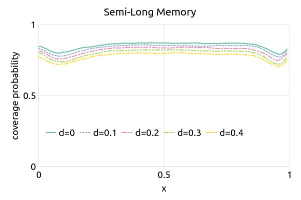
Figure 1: Comparison of coverage probabilities for the regression function $f(x)$ between LM (left) and SLM (right) processes under the assumption of $\rho_{\zeta,\epsilon}=0.5$ for different values of $d$. We assume the bandwidth is $h=N^{-1/3}$ and the tempering parameter for the SLM is $\lambda=N^{-1/6}$.

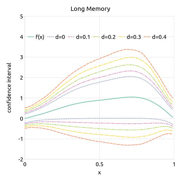
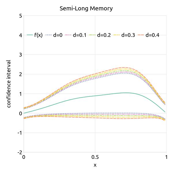
Figure 2: Comparison of empirical confidence intervals for the regression function $f(x)$ between LM (left) and SLM (right) processes under the assumption of $\rho_{\zeta,\epsilon}=0.5$ for different values of $d$. We assume the bandwidth is $h=N^{-1/3}$ and the tempering parameter for the SLM is $\lambda=N^{-1/6}$.

Table 2: Comparison of coverage probabilities and expected lengths of confidence intervals between LM and SLM processes for $f(x)$ given some selected points of $x$ on the interval [0,1], where we assume $\rho_{\zeta,\epsilon}=0.5$. The values in the parentheses are the expected lengths of confidence intervals.

$x$	Regressor	Bandwidth	$d=0$	$d=0.1$	$d=0.2$	$d=0.3$	$d=0.4$
	LM	$N^{-1/3}$	0.854	0.775	0.677	0.588	0.479
			(1.053)	(1.188)	(1.297)	(1.431)	(1.558)
		$N^{-1/5}$	0.926	0.880	0.823	0.760	0.664
			(0.829)	(0.992)	(1.125)	(1.261)	(1.371)
$0.25$	SLM1	$N^{-1/3}$	0.854	0.828	0.790	0.755	0.706
			(1.053)	(1.117)	(1.194)	(1.273)	(1.336)
		$N^{-1/5}$	0.926	0.913	0.893	0.876	0.849
			(0.829)	(0.907)	(0.973)	(1.048)	(1.132)
	SLM3	$N^{-1/3}$	0.854	0.837	0.818	0.797	0.768
			(1.053)	(1.101)	(1.161)	(1.218)	(1.231)
		$N^{-1/5}$	0.926	0.918	0.906	0.896	0.882
			(0.829)	(0.885)	(0.932)	(0.976)	(1.020)

Table 2. (continued)

$x$	Regressor	Bandwidth	$d=0$	$d=0.1$	$d=0.2$	$d=0.3$	$d=0.4$
	LM	$N^{-1/3}$	0.870	0.786	0.696	0.597	0.484
			(1.687)	(1.924)	(2.109)	(2.286)	(2.406)
		$N^{-1/5}$	0.945	0.907	0.860	0.806	0.703
			(1.286)	(1.537)	(1.779)	(1.998)	(2.206)
$0.50$	SLM1	$N^{-1/3}$	0.870	0.838	0.806	0.7693	0.724
			(1.687)	(1.818)	(1.943)	(2.081)	(2.186)
		$N^{-1/5}$	0.945	0.933	0.917	0.902	0.881
			(1.286)	(1.398)	(1.521)	(1.629)	(1.767)
	SLM3	$N^{-1/3}$	0.870	0.851	0.832	0.807	0.786
			(1.687)	(1.768)	(1.860)	(1.944)	(2.010)
		$N^{-1/5}$	0.945	0.936	0.930	0.918	0.910
			(1.286)	(1.359)	(1.472)	(1.506)	(1.596)
	LM	$N^{-1/3}$	0.867	0.779	0.687	0.591	0.483
			(1.926)	(2.165)	(2.353)	(2.646)	(2.852)
		$N^{-1/5}$	0.935	0.897	0.843	0.783	0.681
			(1.326)	(1.580)	(1.818)	(2.056)	(2.226)
$0.75$	SLM1	$N^{-1/3}$	0.867	0.836	0.799	0.762	0.721
			(1.926)	(2.059)	(2.187)	(2.349)	(2.397)
		$N^{-1/5}$	0.935	0.921	0.906	0.885	0.866
			(1.326)	(1.452)	(1.565)	(1.668)	(1.812)
	SLM3	$N^{-1/3}$	0.867	0.850	0.829	0.805	0.779
			(1.926)	(1.996)	(2.098)	(2.200)	(2.301)
		$N^{-1/5}$	0.935	0.928	0.919	0.910	0.895
			(1.326)	(1.411)	(1.488)	(1.559)	(1.633)
	LM	$N^{-1/3}$	0.796	0.701	0.596	0.501	0.397
			(0.855)	(0.974)	(1.032)	(1.160)	(1.240)
		$N^{-1/5}$	0.875	0.833	0.777	0.718	0.623
			(0.989)	(1.183)	(1.377)	(1.568)	(1.733)
$0.95$	SLM1	$N^{-1/3}$	0.796	0.753	0.716	0.672	0.629
			(0.855)	(0.902)	(0.978)	(1.027)	(1.053)
		$N^{-1/5}$	0.875	0.860	0.842	0.822	0.804
			(0.989)	(1.085)	(1.165)	(1.256)	(1.374)
	SLM3	$N^{-1/3}$	0.796	0.773	0.744	0.721	0.690
			(0.855)	(0.907)	(0.921)	(0.957)	(1.009)
		$N^{-1/5}$	0.875	0.870	0.858	0.847	0.831
			(0.989)	(1.045)	(1.118)	(1.161)	(1.234)

Discussion on the application of LM and SLM processes

The strongly tempered process $\eqref{SLMx}$ belongs to the general class of stochastic processes called tempered linear processes, see Sabzikar and Surgailis (2018). These processes have a semi-long memory property in the sense that their autocovariance functions initially resemble that of a long memory process but eventually decay fast at an exponential rate. One special case of such processes is the autoregressive tempered fractionally integrated moving average ARTFIMA$(p,d,\lambda,q)$ process with $p$ as the order of autoregressive polynomial and $q$ as the order of moving average polynomial, which has been studied by Meerschaert et al. (2014) and Sabzikar et al. (2019).

The class of ARTFIMA$(0,d,\lambda,0)$ which does not have autoregressive and moving average components is highly applicable. Some empirical examples include modeling of the log returns for AMZN stock prices, modeling of geophysical turbulence in water velocity data, and modeling of climate data sets given in Sabzikar et al. (2019). In all cases, the authors have found that by using an ARTFIMA model, we are able to capture aspects of the low frequency activity of time series better than an ARFIMA model without the consideration of $\lambda$ in the model.

In practice when analyzing a single data set with size $N$, the tempering parameter $\lambda$ is fixed, and one can use Whittle estimation or maximum likelihood estimation to estimate the unknown parameters $d$ and $\lambda$. These estimators are strongly consistent under general conditions (see Sabzikar et al. (2019)). On the other hand, if one wishes to estimate $\lambda$ as a function of $N$ from a sequence of increasing time series, the problem becomes challenging. This problem could be pursued by developing confidence intervals such that we impose an assumption of $\zeta(s)\sim N(0,1)$ in expression (2) or assume $X_{d,\lambda}(s)=e^{-\lambda}X_{d,\lambda}(s-1)+\xi(s)$ after some algebra, where $\xi(s)$ is a function of $\zeta(s)$’s. This situation is complex and the simplest case is AR(1) setting. Some approaches in this regard are given by Mikusheva (2007) and Phillips (2014). These extensions require complex further calculations which are beyond the scope of the current manuscript (see Remark 3.7 in Sabzikar et al. (2020) for a related argument as well as Section 5 in Sabzikar and Surgailis (2018)). For the simulation studies in this manuscript, we fixed $\lambda$ at multiple points.

The kernel estimator of the unknown regression function $f(x)$ given in (6) depends on the bandwidth $h$. In order to select the bandwidth, note that in the nonstationary case, the amount of time spent by the process around any particular spatial point is of order $\sqrt{N}$ rather than $N$ (see also Wang and Phillips (2009a)). For the practical interest and the nonstationary regressor $x_{k}$ with semi-long memory, the corresponding rate in such regressions is $\{\sqrt{N}\lambda^{d}h\}^{1/2}$ where we require that $\sqrt{N}\lambda^{d}h\rightarrow\infty$. Note that the choice of bandwidth $h$ is related to the nature of the nonstationary regressor $x_{k}$. In our simulations, we found that the rate $h=o(N^{-1/6})$ is sufficient for undersmoothing to remove the asymptotic bias of $\hat{f}(x)$.

Finally, the test statistic $T_{\lambda,d}$ which is discussed in this manuscript, has an asymptotic reference distribution given in Theorem 5.1, which is of complex form and is not easy to be used in practice. The limit distribution of the statistic involves the term $d^{2}_{(0)}$, which does not have a simple form and depends on $x$ through $\hat{\sigma}^{2}_{N}$. Under appropriate conditions, one can approximate the sampling distribution of the test statistic through the use of the subsampling technique given by Politis and Romano (1994), which allows us to be able to study the properties of test statistic under both long memory and semi-long memory input shocks to the regressors. In order to establish the validity of subsampling, one can use the between-block mixing coefficient, which is weaker than the regular $\alpha$-mixing coefficient and is sufficient for strong dependency; see for instance Bai and Taqqu (2017). The extension of subsampling is beyond the scope of this paper, and we leave it for future work.

Conclusion

In this article we have considered the use of tempered or semi-long memory regressor processes within the context of cointegrating regression models for time series analysis. We have developed limit theory that allows the construction of pointwise confidence intervals for a nonlinear regression function when estimation is accomplished through the use of a kernel smoother. We have also demonstrated that the limit distribution of a test statistic for specification of the regression function does not depend on the differencing parameter $d$ under semi-long memory. Through simulation studies we have shown that performance of interval estimators of a regression function is more stable and has generally better performance for the semi-long memory case than for long-memory. It is thus beneficial to use methods based on this theory if it can provide a reasonable framework within which to consider a particular problem.

Appendix A: Technical Details and Proofs

A.1  Preliminaries and Lemmas

$\bullet$ Throughout this section, we set $d_{N}:=[\mathbb{E}(x_{N}^{2})]^{1/2}$. Under the semi-long memory setting, the asymptotic form of $d_{N}$ is given by $d_{N}\sim\sqrt{N}/\lambda^{d}$ as $N\rightarrow\infty$. Then,

$$\frac{x_{N}}{d_{N}}:=\frac{\lambda^{d}}{\sqrt{N}}\sum_{s=1}^{N}X_{d,\lambda}(s)=\frac{1}{\sqrt{N}}\sum_{s=1}^{N}\zeta(s)+o_{P}(1),$$ (A.1)

see expression (A.7) in Sabzikar et al. (2020). For any $t\in[0,1]$, the following weak convergence applies on $D[0,1]$:

$$\frac{x_{\lfloor Nt\rfloor}}{d_{N}}\Rightarrow B(t),$$

where $\lfloor Nt\rfloor$ is the floor function, and $B(t)$ is the standard Brownian motion.

$\bullet$ We decompose $x_{k}$ as follows:

$$x_{k}\equiv\sum_{j=1}^{k}X_{d,\lambda}(j) =\sum_{j=1}^{k}\sum_{i=-\infty}^{j}\phi_{N}(j-i)\zeta(i),\quad\phi_{N}(j):=e^{-\lambda_{N}j}b_{d}(j)$$

$$=x_{s}+\sum_{j=s+1}^{k}\sum_{i=-\infty}^{s}\phi_{N}(j-i)\zeta(i)+\sum_{j=s+1}^{k}\sum_{i=s+1}^{j}\phi_{N}(j-i)\zeta(i)$$

$$=:x^{*}_{s,k}+x^{\prime}_{s,k},\qquad s<k,$$

such that $x^{*}_{s,k}=x_{s}+\sum_{j=s+1}^{k}\sum_{i=-\infty}^{s}\phi_{N}(j-i)\zeta(i)$ and it depends on $\{\cdots,\zeta(s-1),\zeta(s)\}$, and $x^{\prime}_{s,k}=\sum_{j=1}^{k-s}\sum_{i=1}^{j}\phi_{N}(j-i)\zeta(i+s).$ If we define $a_{N}:=\sum_{j=0}^{N}\phi_{N}(j)$, then we can show $a_{N}\asymp O(\lambda^{-d})$ as $N\lambda\rightarrow\infty$ and recall that $\lambda_{N}\equiv\lambda$ is a sample size dependent parameter; see Lemma A.5 part (b) in Sabzikar et al. (2020).

Definition A.1.

Let $\Omega_{N}(\eta)\equiv\{(l,k):\eta N\leq k\leq(1-\eta)N,k+\eta N\leq l\leq N\}$ for all $0\leq k<l\leq N$ and $N\geq 1$, where $0<\eta<1$. A random array $\{x_{k,N}\}_{k\geq 1,N\geq 1}$ is called strong smooth if there exists a sequence of constants $d_{l,k,N}>0$ and a sequence of $\sigma$-fields $\mathcal{F}_{k,N}$ (define $\mathcal{F}_{0,N}=\sigma\{\phi,\Omega\}$, the trivial $\sigma$-field) such that

• For some $m_{0}>0$ and $C>0$, $\inf_{(l,k)\in\Omega_{N}(\eta)}d_{l,k,N}\geq\eta^{m_{0}}/C$ as $N\rightarrow\infty$,

  • $\lim_{\eta\rightarrow 0}\lim_{N\rightarrow\infty}\frac{1}{N}\sum_{l=(1-\eta)N}^{N}(d_{l,0,N})^{-1}=0$,

  • $\lim_{\eta\rightarrow 0}\lim_{N\rightarrow\infty}\frac{1}{N}\max_{0\leq k\leq(1-\eta)N}\sum_{l=k+1}^{k+\eta N}(d_{l,k,N})^{-1}=0$, and

  • $\limsup_{N\rightarrow\infty}\frac{1}{N}\max_{0\leq k\leq N-1}\sum_{l=k+1}^{N}(d_{l,k,N})^{-1}<\infty$.

• $x_{k,N}$ is adapted to $\mathcal{F}_{k,N}$, and conditional on $\mathcal{F}_{k,N}$, $(x_{l,N}-x_{k,N})/d_{l,k,N}$ has a density $h_{l,k,N}(x)$ which is uniformly bounded by a constant $K$ and

  $$\lim_{\kappa\rightarrow 0}\lim_{N\rightarrow\infty}\sup_{(l,k)\in\Omega_{N}(\kappa^{1/(2m_{0})})}\sup_{|u|\leq\kappa}|h_{l,k,N}(u)-h_{l,k,N}(0)|=0.$$

Lemma A.1.

Let’s define $\eta_{i}=(\zeta(i),\epsilon(i))^{\prime}$ where $\mathbb{E}(\eta_{0})=0$ and $\mathbb{E}||\eta_{0}||^{2}<\infty$. Let $\mathcal{F}_{s}=\sigma(\eta_{s},\eta_{s-1},...)$, $\Lambda=\Lambda(\eta_{1},...,\eta_{m_{0}})$ for some $m_{0}>0$ be a real function where $\mathbb{E}(\Lambda(\eta_{1}))=0$, and $g(x)$ is a bounded function such that $\int_{\mathbb{R}}|g(x)|dx<\infty$.

• For a constant $A_{0}$, we have

  $$\sup_{x}\mathbb{E}\Big{|}\sum_{k=1}^{N}g\Big{[}\frac{x_{k}-x}{h}\Big{]}\Big{|}^{m}\leq A_{0}^{m}(m+1)!\,\Big{(}\sqrt{N}\lambda^{d}h\Big{)}^{m},\quad m\geq 1.$$ (A.2)

• As $\{\sqrt{N}\lambda^{d}h\}^{-1}\rightarrow 0$ and $N\lambda\rightarrow\infty$, we have

  $$\sup\limits_{x}\mathbb{E}\Big{|}\sum_{k=1}^{N}\Lambda(\eta_{k-j})g\Big{[}\frac{x_{k}-x}{h}\Big{]}\Big{|}^{2} \leq C\,\mathbb{E}\Lambda^{2}(\eta_{1})\sqrt{N}\lambda^{d}h\,\Big{\{}1+h\sqrt{j}\Big{\}}.$$ (A.3)

• If we define $u_{k}:=\sum_{j=0}^{\infty}\psi_{j}\eta_{k-j}$, then

  $$\mathbb{E}\Big{|}\sum_{k=1}^{N}u_{k}\,g\Big{(}\frac{x_{k}}{h}\Big{)}\Big{|}^{2}\leq C\,\mathbb{E}||\eta_{1}||^{2}\sqrt{N}\lambda^{d}h.$$ (A.4)

• If we define $u_{k,m_{0}}:=\sum_{j=m_{0}}^{\infty}\psi_{j}\Lambda^{\prime}_{k-j}$ where $\psi_{j}=(\psi_{1j},\psi_{2j})$ and $\Lambda_{j}=(\Lambda_{1}(\eta_{j}),\Lambda_{2}(\eta_{j}))$, then we have

  $$\sup_{x}\mathbb{E}\Big{|}\sum_{k=1}^{N}u_{k,m_{0}}\,g\Big{[}x_{k}-\frac{x}{h}\Big{]}\Big{|}^{2}\leq C\,\mathbb{E}||\Lambda_{1}||^{2}\sqrt{N}\lambda^{d}h\,\Big{\{}\sum_{j=m_{0}}^{\infty}j^{1/4}(|\psi_{1j}|+|\psi_{2j}|)\Big{\}}^{2}.$$ (A.5)

Proof.

For the proof of expression (A.2), see Lemma 5.1. of Chan and Wang (2014). To prove (A.3), note that some of the details are very similar to the ones given for the proof of expression (8.11) in Lemma 8.2. of Wang and Phillips (2016), and therefore we only give an outline for the different parts as follows. Let

$$\Delta_{N} \equiv\Big{|}\sum_{k=1}^{N}\Lambda(\eta_{k-j})g\Big{[}\frac{x_{k}-x}{h}\Big{]}\Big{|}^{2}\leq 2\Big{|}\sum_{k=A_{0}}^{N}\Lambda(\eta_{k-j})g\Big{[}\frac{x_{k}-x}{h}\Big{]}\Big{|}^{2}+C\Big{(}\sum_{k=1}^{A_{0}}|\Lambda(\eta_{k-j})|\Big{)}^{2}$$

$$=2\Big{(}\sum_{k=A_{0}}^{N}\sum_{l=1,|k-l|<A_{0}}^{N}+2\sum_{k=A_{0}}^{N-1}\sum_{l=k+A_{0}}^{N}\Big{)}\Lambda(\eta_{k-j})\Lambda(\eta_{l-j})$$

$$\quad\times g\Big{[}\frac{x_{k}-x}{h}\Big{]}g\Big{[}\frac{x_{l}-x}{h}\Big{]}+C\Big{(}\sum_{k=1}^{A_{0}}|\Lambda(\eta_{k-j})|\Big{)}^{2}$$

$$=\Delta_{1N}+\Delta_{2N}+\Delta_{3N},$$

where $A_{0}$ is a positive constant. Then by letting $d_{N}\sim\sqrt{N}/\lambda^{d}$, we have

$$\sup\limits_{x}\mathbb{E}|\Delta_{1N}| \leq C\,\mathbb{E}\Lambda^{2}(\eta_{1})\sqrt{N}\lambda^{d}h,$$

$$\sup\limits_{x}\mathbb{E}|\Delta_{2N}| \leq C\,\mathbb{E}\Lambda^{2}(\eta_{1})h^{2}\sum_{k=A_{0}}^{N-1}d_{k}^{-1}\Big{(}\sum_{l=k+A_{0}}^{N\land(k+j)}d_{l-k}^{-1}+\sum_{k=0}^{j}|\phi_{N}(k)|\sum_{l=k+j}^{N}d_{l-k}^{-2}\Big{)}$$

$$\leq C\,\mathbb{E}\Lambda^{2}(\eta_{1})\sqrt{N}\lambda^{d}h^{2}\Big{(}\frac{j}{d_{j}}+\sum_{k=0}^{j}|\phi_{j}(k)|\sum_{l=k+j}^{N}\frac{\lambda_{l-k}^{2d}}{l-k}\Big{)}$$

$$\leq C\,\mathbb{E}\Lambda^{2}(\eta_{1})\sqrt{N}\lambda^{d}h^{2}\Big{(}\frac{j}{d_{j}}+\sum_{k=0}^{j}|\phi_{j}(k)|\Big{)}$$

$$\leq C\,\mathbb{E}\Lambda^{2}(\eta_{1})\sqrt{N}\lambda^{d}h^{2}\Big{(}\frac{\lambda_{j}^{d}}{\sqrt{j}}j+\lambda_{j}^{-d}\Big{)}$$

$$\leq C\,\mathbb{E}\Lambda^{2}(\eta_{1})\sqrt{N}\lambda^{d}h^{2}\sqrt{j}\quad\text{for}\quad j\geq 1,\quad\text{and}$$

$$\sup\limits_{x}\mathbb{E}|\Delta_{3N}| \leq C\,\mathbb{E}\Lambda^{2}(\eta_{1}).$$

Eventually, we can conclude expression (A.3). Expression (A.4) easily follows from expression (A.3), and expression (A.5) can be followed by a similar path from the proof of expression (8.13) in Lemma 8.2. of Wang and Phillips (2016). ∎

A.2  Proofs of Theorems

Proof of Theorem 4.1. First, in order to establish the asymptotic distribution of $[\hat{f}(x)-f(x)]$, we decompose it as follows:

$$\hat{f}(x)-f(x)=\frac{\sum_{k=1}^{N}u_{k}K[(x_{k}-x)/h]}{\sum_{k=1}^{N}K[(x_{k}-x)/h]}+\frac{\sum_{k=1}^{N}[f(x_{k})-f(x)]K[(x_{k}-x)/h]}{\sum_{k=1}^{N}K[(x_{k}-x)/h]}.$$ (A.6)

Then, only the first term in expression (A.6) determines the asymptotic distribution of $[\hat{f}(x)-f(x)]$ as the second term is negligible under mild conditions. To prove the self-normalized expression (8), let $\Theta_{1N}:=\sum_{k=1}^{N}u_{k}K[\frac{x_{k}-x}{h}]$, $\Theta_{2N}:=\sum_{k=1}^{N}(f(x_{k})-f(x))K[\frac{x_{k}-x}{h}]$, and $\Theta_{3N}:=1/\sum_{k=1}^{N}K[\frac{x_{k}-x}{h}]$. Now, we have

$$\Big{\{}h\sum_{k=1}^{N}K_{h}(x_{k}-x)\Big{\}}^{1/2}\Big{(}\hat{f}(x)-f(x)\Big{)}$$

$$\qquad=\frac{\sum_{k=1}^{N}u_{k}K[(x_{k}-x)/h]}{\{\sum_{k=1}^{N}K[(x_{k}-x)/h]\}^{1/2}}+\frac{\sum_{k=1}^{N}[f(x_{k})-f(x)]K[(x_{k}-x)/h]}{\{\sum_{k=1}^{N}K[(x_{k}-x)/h]\}^{1/2}}$$

$$\qquad=\frac{\Theta_{1N}}{\Theta_{3N}^{-1/2}}+\Theta_{2N}\sqrt{\Theta_{3N}}=\frac{\{\sqrt{N}\lambda^{d}h\}^{-1/2}\,\Theta_{1N}}{\{\sqrt{N}\lambda^{d}h\}^{-1/2}\,\Theta_{3N}^{-1/2}}+\Theta_{2N}\,\,\sqrt{\Theta_{3N}}$$

$$\qquad\rightarrow_{D}\frac{d_{0}\,N(0,1)\,L_{B}^{1/2}(1,0)}{\sqrt{d_{1}}\,L_{B}^{1/2}(1,0)}=\frac{d_{0}}{\sqrt{d_{1}}}N(0,1)=:N(0,\sigma^{2}),$$ (A.7)

where $\sigma^{2}=d_{0}^{2}/d_{1}$. Note that we have used the fact that $\Theta_{2N}\sqrt{\Theta_{3N}}\rightarrow_{P}0$ from Proposition A.8. Also, the last line in (A.7) comes from (a) Slutsky’s theorem, (b) $\{\sqrt{N}\lambda^{d}h\}^{-1}\sum_{k=1}^{\lfloor Nt\rfloor}K[\frac{x_{k}-x}{h}]$
$\rightarrow_{D}d_{1}\,L_{B}(t,0)$, and (c) the following result:

$$\Big{\{}\sqrt{N}\lambda^{d}h\Big{\}}^{-1/2}\sum_{k=1}^{N}K\Big{[}\frac{x_{k}-x}{h}\Big{]}u_{k}\rightarrow_{D}d_{0}\,N(0,1)\,L_{B}^{1/2}(1,0).$$ (A.8)

The convergence in distribution in (A.8) comes from Proposition A.9 part (iv). Expression (8) easily implies expression (7) and the fact that

$$\Big{\{}\sqrt{N}\lambda^{d}h\Big{\}}^{1/2}\Big{(}\hat{f}(x)-f(x)\Big{)} =\Big{\{}\sqrt{N}\lambda^{d}h\Big{\}}^{1/2}\frac{\{h\sum_{k=1}^{N}K_{h}(x_{k}-x)\}^{1/2}(\hat{f}(x)-f(x))}{\{h\sum_{k=1}^{N}K_{h}(x_{k}-x)\}^{1/2}}$$

$$\rightarrow_{D}\frac{d_{0}}{\sqrt{d_{1}}}\,L_{B}^{-1/2}(1,0)\,N(0,1),$$

thus the proof is complete. $\square$

Proof of Theorem 5.1. First, $T_{N}$ can be decomposed into three terms under $H_{0}$, i.e. $y_{k}=g(x_{k},\theta_{0})+u_{k}$, as follows

$$T_{N} =\int_{\mathbb{R}}\Big{\{}\sum_{k=1}^{N}K\Big{[}\frac{x_{k}-x}{h}\Big{]}\Big{[}g(x_{k},\theta_{0})+u_{k}-g(x_{k},\hat{\theta}_{N})\Big{]}\Big{\}}^{2}\pi(x)dx$$

$$=T_{N}^{\text{I}}+T_{N}^{\text{II}}+T_{N}^{\text{III}},\quad\text{such that}$$

$$T_{N}^{\text{I}} :=\int_{\mathbb{R}}\Big{\{}\sum_{k=1}^{N}K\Big{[}\frac{x_{k}-x}{h}\Big{]}u_{k}\Big{\}}^{2}\pi(x)dx,$$

$$T_{N}^{\text{II}} :=\int_{\mathbb{R}}\Big{\{}\sum_{k=1}^{N}K\Big{[}\frac{x_{k}-x}{h}\Big{]}\Big{(}g(x_{k},\theta_{0})-g(x_{k},\hat{\theta}_{N})\Big{)}\Big{\}}^{2}\pi(x)dx,\quad\text{and}$$

$$T_{N}^{\text{III}} :=2\int_{\mathbb{R}}\Big{\{}\sum_{1\leq k<j\leq N}K\Big{[}\frac{x_{k}-x}{h}\Big{]}K\Big{[}\frac{x_{j}-x}{h}\Big{]}u_{k}\Big{(}g(x_{j},\theta_{0})-g(x_{j},\hat{\theta}_{N})\Big{)}\Big{\}}\pi(x)dx.$$

Based on Assumption 5.2, there exists $g_{1}(x)$ such that for each $\theta,\theta_{0}\in\Theta$, we have $|g(x,\theta)-g(x,\theta_{0})|\leq C||\theta-\theta_{0}||g_{1}(x)$. Therefore,

$$T_{N}^{\text{II}}\leq C||\hat{\theta}_{N}-\theta_{0}||^{2}\int_{\mathbb{R}}\Big{\{}\sum_{k=1}^{N}K\Big{[}\frac{x_{k}-x}{h}\Big{]}g_{1}(x_{k})\Big{\}}^{2}\pi(x)dx=o_{P}\Big{(}\sqrt{N}\lambda^{d}h\Big{)}.$$ (A.9)

Expression (A.9) comes from (a) Assumption 5.3, $||\hat{\theta}_{N}-\theta_{0}||=o_{P}(\{\sqrt{N}\lambda^{d}h\}^{-1/2})$ and (b) the following result:

$$\Big{\{}\sqrt{N}\lambda^{d}h\Big{\}}^{-2}\int_{\mathbb{R}}\Big{\{}\sum_{k=1}^{N}K\Big{[}\frac{x_{k}-x}{h}\Big{]}m(x_{k})\Big{\}}^{2}\pi(x)dx\rightarrow_{D}\frac{d_{(1)}^{2}}{d_{1}}L_{B}^{2}(1,0),$$ (A.10)

where $d^{2}_{(1)}=\int_{\mathbb{R}}m^{2}(x)\pi(x)dx\int_{\mathbb{R}}K(s)ds$ and $d_{1}=\int_{\mathbb{R}}K(s)ds$. Expression (A.10) can be obtained by a similar path from the expression (7.12) in Proposition 7.3 of Wang and Phillips (2016).

For a fixed $A>0$, we define the followings: $\hat{\eta_{i}}=\eta_{i}\,I(||\eta_{i}||\leq A)$, $\tilde{\eta}_{i}=\hat{\eta}_{i}-\mathbb{E}(\hat{\eta}_{i})$, $\mathring{\eta}_{i}=\eta_{i}-\tilde{\eta}_{i}$, $\tilde{u}_{k}=\sum_{j=0}^{\infty}\psi_{j}\tilde{\eta}_{k-j}$, and $\mathring{u}_{k}=\sum_{j=0}^{\infty}\psi_{j}\mathring{\eta}_{k-j}$. Let $u_{k}=\tilde{u}_{k}+\mathring{u}_{k}$, $\tilde{u}_{1k}=\sum_{j=0}^{m_{0}}\psi_{j}\tilde{\eta}_{k-j}$, and $\tilde{u}_{2k}=\tilde{u}_{k}-\tilde{u}_{1k}$. Also, note that

$$\sum_{1\leq k<j\leq N}\tilde{u}_{1k}\tilde{u}_{1j}\Big{\{}\int_{\mathbb{R}}K\Big{[}\frac{x_{k}-x}{h}\Big{]}K\Big{[}\frac{x_{j}-x}{h}\Big{]}\pi(x)dx\Big{\}}=o_{P}\Big{(}\sqrt{N}\lambda^{d}h\Big{)},$$ (A.11)

which can be followed by a similar path from the proof of expression (8.18) in Lemma 8.3 of Wang and Phillips (2016). Therefore, we can conclude $T_{N}^{\text{III}}=o_{P}(\sqrt{N}\lambda^{d}h)$. Now, it suffices to show $\{\sqrt{N}\lambda^{d}h\}^{-1}T_{N}^{\text{I}}\rightarrow_{D}d^{2}_{(0)}L_{B}(1,0)$. From expression (A.5) of Lemma A.1, we have

$$\mathbb{E}\int_{\mathbb{R}}\Big{\{}\sum_{k=1}^{N}K\Big{[}\frac{x_{k}-x}{h}\Big{]}\mathring{u}_{k}\Big{\}}^{2}\pi(x)dx\leq C\,\mathbb{E}||\mathring{\eta}_{1}||^{2}\,\sqrt{N}\lambda^{d}h\leq C\,\mathbb{E}||\eta_{1}||^{2}I(||\eta_{1}||>A)\sqrt{N}\lambda^{d}h,$$

where $\mathbb{E}(\mathring{\eta}_{1})=0$. Note that $\mathbb{E}||\eta_{1}||^{2}I(||\eta_{1}||>A)\rightarrow 0$ as $A\rightarrow\infty$, therefore it suffices to show

$$\Big{\{}\sqrt{N}\lambda^{d}h\Big{\}}^{-1}T_{N}^{\text{I}}:=\Big{\{}\sqrt{N}\lambda^{d}h\Big{\}}^{-1}\int_{\mathbb{R}}\Big{\{}\sum_{k=1}^{N}K\Big{[}\frac{x_{k}-x}{h}\Big{]}\tilde{u}_{k}\Big{\}}^{2}\pi(x)dx\rightarrow_{D}d^{2}_{(0)}L_{B}(1,0).$$

Then, we have $T_{N}^{\text{I}}=T^{\text{I}(a)}_{N}+T^{\text{I}(b)}_{N}+T^{\text{I}(c)}_{N}$ where

$$T^{\text{I}(a)}_{N} =\int_{\mathbb{R}}\Big{\{}\sum_{k=1}^{N}K\Big{[}\frac{x_{k}-x}{h}\Big{]}\tilde{u}_{1k}\Big{\}}^{2}\pi(x)dx,$$

$$T^{\text{I}(b)}_{N} =\int_{\mathbb{R}}\Big{\{}\sum_{k=1}^{N}\Big{[}\frac{x_{k}-x}{h}\Big{]}\tilde{u}_{2k}\Big{\}}^{2}\pi(x)dx,\quad\text{and}$$

$$T^{\text{I}(c)}_{N} =2\int_{\mathbb{R}}\Big{\{}\sum_{1\leq k<j\leq N}K\Big{[}\frac{x_{k}-x}{h}\Big{]}K\Big{[}\frac{x_{j}-x}{h}\Big{]}\tilde{u}_{1k}\tilde{u}_{2k}\Big{\}}\,\pi(x)dx.$$

Now based on expression (A.5) in Lemma A.1, we have

$$\mathbb{E}(T^{\text{I}(b)}_{N}) \leq C\,\sup_{x}\mathbb{E}\Big{\{}\sum_{k=1}^{N}K\Big{[}\frac{x_{k}-x}{h}\Big{]}\tilde{u}_{2k}\Big{\}}^{2}$$

$$\leq C\,\mathbb{E}||\eta_{1}||^{2}\sqrt{N}\lambda^{d}h\,\Big{\{}\sum_{k=m_{0}}^{\infty}k^{1/4}(|\psi_{1k}|+|\psi_{2k}|)\Big{\}}^{2},\quad\text{as}\quad N\rightarrow\infty\quad\text{and}\quad m_{0}\rightarrow 0.$$

Under Assumption 4.1, $\sum_{k=m_{0}}^{\infty}k^{1/4}(|\psi_{1k}|+|\psi_{2k}|)<\infty$. Therefore, we conclude $T^{\text{I}(b)}_{N}=o_{P}(\sqrt{N}\lambda^{d}h)$. Based on expression (A.11), $T^{\text{I}(c)}_{N}=o_{P}(\sqrt{N}\lambda^{d}h)$. We can furtherly write $T^{\text{I}(a)}_{N}$ as

$$T^{\text{I}(a)}_{N} =\int_{\mathbb{R}}\Big{\{}\sum_{k=1}^{N}K\Big{[}\frac{x_{k}-x}{h}\Big{]}\tilde{u}_{1k}\Big{\}}^{2}\pi(x)dx=\mathbb{E}(\tilde{u}_{10}^{2})\sum_{k=1}^{N}\int_{\mathbb{R}}K^{2}\Big{[}\frac{x_{k}-x}{h}\Big{]}\pi(x)dx$$

$$\quad+\sum_{k=1}^{N}(\tilde{u}^{2}_{1k}-\mathbb{E}(\tilde{u}_{1k}^{2}))\int_{\mathbb{R}}K^{2}\Big{[}\frac{x_{k}-x}{h}\Big{]}\pi(x)dx$$

$$\quad+2\sum_{1\leq k<j\leq N}\tilde{u}_{1k}\tilde{u}_{1j}\int_{\mathbb{R}}K\Big{[}\frac{x_{k}-x}{h}\Big{]}K\Big{[}\frac{x_{j}-x}{h}\Big{]}\pi(x)dx$$

$$=R^{\text{I}(a)}_{N}+R^{\text{II}(a)}_{N}+R^{\text{III}(a)}_{N}.$$

From

$$\sum_{k=1}^{N}\Big{(}\tilde{u}^{2}_{1k}-\mathbb{E}(\tilde{u}^{2}_{1k})\Big{)}\int_{\mathbb{R}}K^{2}\Big{[}\frac{x_{k}-x}{h}\Big{]}\pi(x)dx=O_{P}\Big{(}\{\sqrt{N}\lambda^{d}h\}^{1/2}\Big{)},$$

which can be followed by a similar path from the expression (8.17) in Lemma 8.3 of Wang and Phillips (2016) and expression (A.11), we can conclude $|R^{\text{II}(a)}_{N}|+|R^{\text{III}(a)}_{N}|=o_{P}(\sqrt{N}\lambda^{d}h)$. Eventually, by virtue of $\mathbb{E}(\tilde{u}_{10}^{2})\rightarrow\mathbb{E}(\tilde{u}_{0}^{2})$, we only need to prove

$$\Big{\{}\sqrt{N}\lambda^{d}h\Big{\}}^{-1}R^{\text{I}(a)}_{N}\rightarrow_{D}\mathbb{E}(\tilde{u}_{0}^{2})\int_{\mathbb{R}}K^{2}(x)dx\int_{\mathbb{R}}\pi(s)ds\,L_{B}(1,0).$$ (A.12)

If we define $\int_{\mathbb{R}}g_{h}(y)dy=\int_{\mathbb{R}}K^{2}(z)dz\int_{\mathbb{R}}\pi(x)dx$ such that $|g_{h}(y)|\leq C\int_{\mathbb{R}}|\pi(x)|dx<\infty$, then (A.12) could be followed from the proof of Theorem 2.1 in Wang and Phillips (2009a), and we omit it. Therefore, the proof is complete. $\square$

Proof of Theorem 5.2. The proof is similar to the proof of Theorem 3.2 in Wang and Phillips (2016). Therefore, we give an outline. We first decompose $T_{N}$ under $H_{A}$, i.e. $y_{k}=g(x_{k},\theta_{0})+\rho_{N}m(x_{k})+u_{k}$ as follows:

$$T_{N} =\int_{\mathbb{R}}\Big{\{}\sum_{k=1}^{N}K\Big{[}\frac{x_{k}-x}{h}\Big{]}\Big{[}g(x_{k},\theta_{0})+\rho_{N}m(x_{k})+u_{k}-g(x_{k},\hat{\theta}_{N})\Big{]}\Big{\}}^{2}\pi(x)dx$$

$$=T_{N}^{\text{I}}+T_{N}^{\text{II}}+T_{N}^{\text{III}}+2\rho_{N}T_{N}^{\text{IV}}+\rho_{N}^{2}T_{N}^{\text{V}},$$

where

$$T_{N}^{\text{IV}} :=\int_{\mathbb{R}}\Big{\{}\sum_{1\leq k<j\leq N}K\Big{[}\frac{x_{k}-x}{h}\Big{]}K\Big{[}\frac{x_{j}-x}{h}\Big{]}m(x_{k})\Big{[}u_{j}-\Big{(}g(x_{j},\hat{\theta}_{N})-g(x_{j},\theta_{0})\Big{)}\Big{]}\Big{\}}\,\pi(x)dx,\,\text{and}$$

$$T_{N}^{\text{V}} :=\int_{\mathbb{R}}\Big{\{}\sum_{k=1}^{N}K\Big{[}\frac{x_{k}-x}{h}\Big{]}m(x_{k})\Big{\}}^{2}\pi(x)dx,$$

such that $|T_{N}^{\text{IV}}|\leq[T_{N}^{\text{I}}+T_{N}^{\text{II}}+T_{N}^{\text{III}}]^{1/2}\times[T_{N}^{\text{V}}]^{1/2}$ by Hölder’s inequality. The remained terms have been already defined in the proof of Theorem 5.1. From the proof of Theorem 5.1, $T_{N}^{\text{I}}+T_{N}^{\text{II}}+T_{N}^{\text{III}}=O_{P}(\sqrt{N}\lambda^{d}h)$. Following Proposition A.9 part (iv), $\{\sqrt{N}\lambda^{d}h\}^{-1}\sum_{k=1}^{N}K(\frac{x_{k}}{h})$ $\rightarrow_{D}L_{B}(1,0)$ under the assumption of $\int_{\mathbb{{R}}}K(x)dx=1$. Therefore, from continuous mapping theorem and expression (A.2), we have $\{\sqrt{N}\lambda^{d}h\}^{-2}T_{N}^{\text{V}}\rightarrow_{D}d_{(1)}^{2}\,L_{B}^{2}(1,0)$, where $d_{(1)}^{2}=\int_{\mathbb{R}}m^{2}(x)\pi(x)dx$, and $P(0<L^{2}_{B}(1,0)<\infty)=1$. We conclude that for any $T_{0}>0$ and as $N\rightarrow\infty$, the following holds

$$\lim\limits_{N\rightarrow\infty}P\Big{(}\{\sqrt{N}\lambda^{d}h\}^{-1}T_{N}\geq T_{0}\Big{)}\geq\lim\limits_{N\rightarrow\infty}P\Big{(}\{\sqrt{N}\lambda^{d}h\}^{-2}T_{N}^{\text{V}}\geq\epsilon_{N}^{-1/4}\Big{)}=1,$$

under the assumption of $\epsilon_{N}:=\sqrt{N}\lambda^{d}h\rho_{N}^{2}\rightarrow\infty$.

Note that $\{\sqrt{N}\lambda^{d}h\}^{-2}T_{N}^{V}\rightarrow_{D}d_{(1)}^{2}\,L_{B}^{2}(1,0)>0$ a.s., which confirms the divergence of $\{\sqrt{N}\lambda^{d}h\}^{-1}T_{N}$ and the test consistency under $H_{A}$. $\square$

A.3  Propositions and Their Proofs

We provide several propositions in this section. These propositions are required for the proofs of theorems 4.1, 5.1, and 5.2 given in the paper.

Proposition A.1.

Let $x_{k,N}=x_{k}/d_{N}$. A random array $\{x_{k,N}\}_{k\geq 1,N\geq 1}$ is called strong smooth.

Proof.

We verify this proposition from the Definition A.1. Assume $\{x_{k,N}\}_{k\geq 1,N\geq 1}$ is a random triangular array such that $x_{0,N}\equiv 0$. Let $d_{l,k}\equiv\lambda_{l-k}^{-d}\,(l-k)^{1/2}$, therefore

$$d_{l,k,N}\equiv\frac{d_{l,k}}{d_{N}}\propto\Big{(}\frac{\lambda_{l-k}}{\lambda_{N}}\Big{)}^{-d}\,\sqrt{\frac{l-k}{N}},\qquad N\lambda_{N}\rightarrow\infty.$$

Recall that $\lambda_{N}\equiv\lambda>0$ is a sample size dependent parameter.

• $\inf_{(l,k)\in\Omega_{N}(\eta)}d_{l,k,N}\equiv\inf_{(l,k)\in\Omega_{N}(\eta)}(\lambda_{l-k}/\lambda_{N})^{-d}\sqrt{(l-k)/N}\geq\sqrt{\frac{\eta N}{N}}\lambda_{\eta N/N}^{d}>0$.

(i) $$\lim_{\eta\rightarrow 0}\lim_{N\rightarrow\infty}\frac{1}{N}\sum_{l=(1-\eta)N}^{N}\Big{\{}\Big{(}\frac{\lambda_{l}}{\lambda_{N}}\Big{)}^{-d}\sqrt{l/N}\Big{\}}^{-1}$$

$$\quad\leq\lim_{\eta\rightarrow 0}\lim_{N\rightarrow\infty}\frac{1}{\sqrt{N}\lambda_{N}^{d}}\int_{(1-\eta)N}^{N}\frac{\lambda_{l}^{d}}{\sqrt{l}}dl$$

$$\quad\leq\lim_{\eta\rightarrow 0}\lim_{N\rightarrow\infty}\frac{1}{\sqrt{N}\lambda_{N}^{d}}\Big{\{}\sqrt{N}\lambda_{N}^{d}-\sqrt{(1-\eta)N}\lambda_{(1-\eta)N}^{d}\Big{\}}=0.$$

(ii) $$\lim_{\eta\rightarrow 0}\lim_{N\rightarrow\infty}\frac{1}{N}\max_{0\leq k\leq(1-\eta)N}\sum_{l=k+1}^{k+\eta N}\Big{\{}\Big{(}\frac{\lambda_{l-k}}{\lambda_{N}}\Big{)}^{-d}\sqrt{(l-k)/N}\Big{\}}^{-1}$$

$$\leq\lim_{\eta\rightarrow 0}\lim_{N\rightarrow\infty}\frac{1}{\sqrt{N}\lambda_{N}^{d}}\max\limits_{0\leq k\leq(1-\eta)N}\int_{k+1}^{k+\eta N}\frac{\lambda_{l-k}^{d}}{\sqrt{l-k}}dl$$

$$=\lim_{\eta\rightarrow 0}\lim_{N\rightarrow\infty}\frac{1}{\sqrt{N}\lambda_{N}^{d}}\Big{\{}\sqrt{\eta N}\lambda_{\eta N}^{d}-1\Big{\}}=0.$$

(iii) $$\limsup\limits_{N\rightarrow\infty}\frac{1}{N}\max\limits_{0\leq k\leq N-1}\sum\limits_{l=k+1}^{N}\Big{\{}\Big{(}\frac{\lambda_{l-k}}{\lambda_{N}}\Big{)}^{-d}\sqrt{(l-k)/N}\Big{\}}^{-1}$$

$$\quad\leq\limsup_{N\rightarrow\infty}\frac{1}{\sqrt{N}\lambda_{N}^{d}}\max\limits_{0\leq k\leq N-1}\int_{k+1}^{N}\frac{\lambda_{l-k}^{d}}{\sqrt{l-k}}dl$$

$$\quad\leq\limsup\limits_{N\rightarrow\infty}\frac{1}{\sqrt{N}\lambda_{N}^{d}}\max\limits_{0\leq k\leq N-1}\Big{\{}\sqrt{N-k}\lambda_{N-k}^{d}-1\Big{\}}$$

$$\quad=\limsup\limits_{N\rightarrow\infty}\Big{\{}1-\frac{1}{\sqrt{N}\lambda_{N}^{d}}\Big{\}}=1<\infty.$$

• If we define $f_{l,k,N}(t)=\mathbb{E}\Big{(}e^{it[x_{l,N}-x_{k,N}]/d_{l,k,N}}\Big{)}$, then

  $$\sup\limits_{x\in\mathbb{R}}\Big{|}h_{l,k,N}(x)-n(x)\Big{|}\leq C\int_{\mathbb{R}}\Big{|}f_{l,k,N}(t)-e^{-t^{2}/2}\Big{|}dt\rightarrow 0,$$

where $n(x)=e^{-x^{2}/2}\big{/}\sqrt{2\pi}$ is the density of standard normal (see proof of Corollary 2.2 in Wang and Phillips (2009a) for a similar argument). Thus, all the conditions given in Definition A.1 hold, and ${x_{k,N}}$ is a strong smooth array. The alternative way to prove this proposition is to use expression (A.1), where $\{\zeta(k)\}_{k\in\mathbb{Z}}$ is a sequence of i.i.d. random variables with $\mathbb{E}(\zeta(0))=0$ and $\mathbb{E}(\zeta^{2}(0))=1$; see expression (A.7) in Sabzikar et al. (2020). Secondly, the triangular array $N^{-1/2}\sum_{k=1}^{N}\zeta(k)$ satisfies the strong smooth conditions; see Wang and Phillips (2009a). This together with (A.1) can complete the proof of Proposition A.1. ∎

Proposition A.2.

Let

$$S_{N}(t)=\frac{1}{[\sqrt{N}h]^{1/2}}\sum\limits_{k=1}^{\lfloor Nt\rfloor}u_{k}K\Big{[}\frac{x_{k}-x}{h}\Big{]},\quad\text{and}\quad\psi_{N}(t)=\frac{1}{\sqrt{N}h}\sum\limits_{k=1}^{\lfloor Nt\rfloor}u^{2}_{k}K^{2}\Big{[}\frac{x_{k}-x}{h}\Big{]}.$$

For any fixed $0\leq t\leq 1$, $S_{N}(t)$, $S^{2}_{N}(t)$, and $\psi_{N}(t)$ are uniformly integrable.

Proof.

The proof is similar to the Proposition 7.3 in Wang and Phillips (2009b); hence, we only give an outline. If we let

$$\psi_{N}^{\prime\prime}(t)=\frac{1}{\sqrt{N}h}\sum_{k=1}^{\lfloor Nt\rfloor}K^{2}\Big{[}\frac{x_{k}-x}{h}\Big{]}\mathbb{E}(u_{k}^{2}),$$

for $0\leq t\leq 1$ and define $r_{y}(t):=K^{2}(\frac{y}{h}+t)$, then $\sup_{N}\mathbb{E}[\psi^{\prime\prime}_{N}(t)]^{2}<\infty$ as follows

$$\mathbb{E}[\psi^{\prime\prime}_{N}(t)]^{2} =\mathbb{E}\Big{\{}\frac{1}{\sqrt{N}h}\sum_{k=1}^{\lfloor Nt\rfloor}K^{2}\Big{[}\frac{x_{k}-x}{h}\Big{]}\mathbb{E}(u_{k}^{2})\Big{\}}^{2}$$

$$\leq\frac{C}{Nh^{2}}\Big{\{}\sum_{k=1}^{N}\mathbb{E}\Big{\{}K^{4}\Big{[}\frac{x_{k}-x}{h}\Big{]}\Big{\}}+2\sum_{1\leq k<l\leq N}\mathbb{E}\Big{\{}K^{2}\Big{[}\frac{x_{k}-x}{h}\Big{]}K^{2}\Big{[}\frac{x_{l}-x}{h}\Big{]}\Big{\}}\Big{\}}$$

$$\leq\frac{C}{Nh^{2}}\Big{\{}\sum_{k=1}^{N}\sup_{y}\mathbb{E}r^{2}_{y}\Big{(}\frac{x^{\prime}_{0,k}}{h}\Big{)}+2\sum_{1\leq k<l\leq N}\sup_{y}\mathbb{E}r_{y}\Big{(}\frac{x^{\prime}_{0,k}}{h}\Big{)}\sup_{y}\mathbb{E}r_{y}\Big{(}\frac{x^{\prime}_{k,j}}{h}\Big{)}\Big{\}}$$

$$\leq\frac{C}{Nh^{2}}\Big{\{}\sum_{k=1}^{N}\frac{h}{\sqrt{k}}+2\sum_{1\leq k<l\leq N}\frac{h^{2}}{\sqrt{k}\sqrt{l-k}}\Big{\}}<\infty,$$

uniformly on $N$. The last line could be followed by a similar path from the proof of Lemma 7.1 part (a) in Wang and Phillips (2009b). Note that $\sup_{0\leq t\leq 1}\mathbb{E}|\psi_{N}(t)-\psi_{N}^{\prime\prime}(t)|^{2}=o(1)$, which can be verified by a similar argument given in Proposition A.6. This implies $\sup_{N}\mathbb{E}[\psi_{N}(t)]^{2}<\infty$, and therefore $\psi_{N}(t)$ is uniformly integrable. Furthermore, we can write

$$|\psi_{N}(t)-S^{2}_{N}(t)|=\frac{2}{\sqrt{N}h}\sum\limits_{1\leq k<l\leq\lfloor Nt\rfloor}u_{k}u_{l}K\Big{[}\frac{x_{k}-x}{h}\Big{]}K\Big{[}\frac{x_{l}-x}{h}\Big{]},$$

which implies $\sup_{0\leq t\leq 1}\mathbb{E}|\psi_{N}(t)-S^{2}_{N}(t)|=o(1)$ and can be verified by a similar argument given in Proposition A.6. Therefore, $S^{2}_{N}(t)$ is uniformly integrable, which implies $S_{N}(t)$ is uniformly integrable. ∎

Proposition A.3.

Let $\Theta_{1N}:=\sum_{k=1}^{N}u_{k}K[\frac{x_{k}-x}{h}]$. Then, $\Theta_{1N}=O_{P}(\{\sqrt{N}h\}^{1/2})$.

Proof.

Based on the Proposition A.2, uniformly in $N$, we have $\mathbb{E}S^{2}_{N}(1)\leq C$, where $C$ is a generic constant. Therefore, based on the Markov’s inequality

$$P(\Theta_{1N}\geq\{\sqrt{N}h\}^{1/2})\leq\frac{\mathbb{E}(\Theta^{2}_{1N})}{\sqrt{N}h}=\mathbb{E}S^{2}_{N}(1)\leq C.$$

As a result, $\Theta_{1N}=O_{P}(\{\sqrt{N}h\}^{1/2})$. ∎

Proposition A.4.

Let $\Theta_{2N}:=\sum_{k=1}^{N}[f(x_{k})-f(x)]K[(x_{k}-x)/h]$. Then, $\Theta_{2N}=O_{P}(Nh^{\gamma+1}/d_{N})$ where $d_{N}=\sqrt{N}/\lambda^{d}$.

Proof.

$$\mathbb{E}|\Theta_{2N}| \leq\sum_{k=1}^{N}\mathbb{E}\Big{\{}|f(x_{k,N}d_{N})-f(x)|K\Big{[}\frac{x_{k,N}d_{N}-x}{h}\Big{]}\Big{\}}$$

$$=\sum_{k=1}^{N}\int_{\mathbb{R}}\Big{\{}|f(d_{N}d_{k,0,N}y)-f(x)|\times K\Big{(}\frac{d_{N}d_{k,0,N}y}{h}-\frac{x}{h}\Big{)}\Big{\}}h_{k,0,N}(y)dy$$

$$\leq\frac{h}{d_{N}}\sum_{k=1}^{N}\frac{1}{d_{k,0,N}}\int_{\mathbb{R}}\{|f(hy+x)-f(x)|K(y)\}dy$$

$$\leq\frac{Nh^{\gamma+1}}{d_{N}}\frac{1}{N}\sum_{k=1}^{N}\frac{1}{d_{k,0,N}}\int_{\mathbb{R}}K(s)f_{1}(s,x)ds\leq A\frac{Nh^{\gamma+1}}{d_{N}},$$

where $A$ is a constant and $\gamma\in(0,1]$. The last line of proof follows from Assumption 4.3 and note that we have considered $x_{k,N}=d_{k,0,N}y$ and $d_{N}d_{k,0,N}y=hy+x$. Therefore, $\Theta_{2N}=O_{P}(Nh^{\gamma+1}/d_{N})$. ∎

Proposition A.5.

Let $\Theta_{3N}:=\{\sum_{k=1}^{N}K[(x_{k}-x)/h]\}^{-1}$. Then, $\Theta_{3N}=o_{P}(\{\sqrt{N}\lambda^{d}h\}^{-1})$.

Proof.

From Proposition A.4, we can easily conclude this under the assumption of $\sqrt{N}\lambda^{d}h\rightarrow\infty$. ∎

Proposition A.6.

Assume $h\rightarrow 0$ and $\sqrt{N}\lambda^{d}h\rightarrow\infty$. Let

$$T_{iN}(t):=\{\sqrt{N}\lambda^{d}h\}^{-1}\sum_{k=1}^{\lfloor Nt\rfloor}K^{i}\Big{[}\frac{x_{k}-x}{h}\Big{]},\quad\text{and}\quad T^{\prime}_{iN}(t):=\{\sqrt{N}\lambda^{d}h\}^{-1}\sum_{k=1}^{\lfloor Nt\rfloor}K^{2}\Big{[}\frac{x_{k}-x}{h}\Big{]}u^{2}_{k}.$$

Then, $T_{iN}(t)\rightarrow_{D}d_{i}L_{B}(t,0)$ and $T^{\prime}_{iN}(t)\rightarrow_{D}d_{0}^{2}L_{B}(t,0)$ for $i=1,2$, where $d_{i}=\int_{\mathbb{R}}K^{i}(s)ds$ and $d_{0}^{2}=\mathbb{E}(u^{2}_{0})\int_{\mathbb{R}}K^{2}(s)ds$.

Proof.

Let’s define $x_{k,N}:=\hat{\xi}_{N}(k/N)$ for $1\leq k\leq N$ such that $\hat{\xi}_{N}(t)\Rightarrow B(t)$ on $D[0,1]$ following Theorem 4.3 in Sabzikar and Surgailis (2018). There exists an equivalent process $\hat{\xi}_{N}(k/N)$ of $\xi_{N}(k/N)$ i.e. $\hat{\xi}_{N}(k/N)=_{D}\xi_{N}(k/N)$ such that $\sup_{0\leq t\leq 1}|\hat{\xi}_{N}(t)-B(t)|=o_{P}(1)$. Now, apply part (i) of Proposition A.9 by setting $c_{N}=\frac{d_{N}}{h}$ and $g(t)=K^{i}[t-\frac{x}{h}]$ for $i=1,2$; then we have

$$\sup\limits_{0\leq t\leq 1}\Big{|}\{\sqrt{N}\lambda^{d}h\}^{-1}\sum_{k=1}^{\lfloor Nt\rfloor}K^{i}\Big{[}\frac{d_{N}\hat{\xi}_{N}(k/N)-x}{h}\Big{]}-L_{B}(t,0)\int_{\mathbb{R}}K^{i}(s)ds\Big{|}\rightarrow_{P}0,$$ (A.13)

as $c_{N}\rightarrow\infty$, $\frac{c_{N}}{N}\rightarrow 0$, and $N\rightarrow\infty$. This together with the fact that $\hat{\xi}_{N}(\frac{k}{N})=_{D}\xi_{N}(\frac{k}{N})=\frac{x_{k}}{d_{N}}$ for $1\leq k\leq N$ imply for $N\geq 1$, $T_{iN}(t)$ is f.d.d. for $d_{i}L_{B}(t,0)$. Additionally, $T_{iN}(t)$ is tight for $N\geq 1$ following Proposition A.7, i.e.

$$\max\limits_{1\leq k\leq N}\Big{|}K^{i}\Big{[}\frac{x_{k}-x}{h}\Big{]}\Big{|}=o_{P}\Big{(}\sqrt{N}\lambda^{d}h\Big{)},$$

under the assumption of $\sup_{0\leq t\leq 1}|x_{\lfloor Nt\rfloor,N}-B(t)|=o_{P}(1)$. Therefore,

$$T_{iN}(t)\rightarrow_{D}d_{i}\,L_{B}(t,0)\quad\text{for}\quad i=1,2.$$

Now, in order to prove $T^{\prime}_{iN}(t):=\{\sqrt{N}\lambda^{d}h\}^{-1}\sum_{k=1}^{\lfloor Nt\rfloor}K^{2}[\frac{x_{k}-x}{h}]u^{2}_{k}\rightarrow_{D}d_{0}^{2}\,L_{B}(t,0)$, we define

$$T_{iN}^{\prime\prime}(t):=\{\sqrt{N}\lambda^{d}h\}^{-1}\sum_{k=1}^{\lfloor Nt\rfloor}K^{2}\Big{[}\frac{x_{k}-x}{h}\Big{]}\mathbb{E}u^{2}_{k},$$

and need to show $\sup_{0\leq t\leq 1}\mathbb{E}|T^{\prime}_{iN}(t)-T^{\prime\prime}_{iN}(t)|^{2}=o(1)$. Based on the Preliminary given in Section A.1, $x_{k}=x^{*}_{0,k}+x^{\prime}_{0,k}$ for $s=0$, we have:

$$\mathbb{E}\Big{[}\Big{|}T^{\prime}_{iN}(t)-T^{\prime\prime}_{iN}(t)\Big{|}^{2}\Big{|}\zeta(0),\zeta(-1),...\Big{]}$$

$$\quad\leq\Big{\{}\frac{1}{\sqrt{N}\lambda^{d}h}\Big{\}}^{2}\sup\limits_{y,1\leq M\leq N}\mathbb{E}\Big{[}\sum_{k=1}^{M}K^{2}\Big{[}\frac{y+x^{\prime}_{0,k}}{h}\Big{]}(u^{2}_{k}-\mathbb{E}(u^{2}_{k}))^{2}\Big{]}^{2}\quad\text{a.s.}$$

$$\quad\leq\Big{\{}\frac{1}{\sqrt{N}\lambda^{d}h}\Big{\}}^{2}\sup\limits_{y}\Big{[}\sum_{k=1}^{N}\mathbb{E}r^{2}\Big{(}\frac{x^{\prime}_{0,k}}{h}\Big{)}g^{2}(u_{k})+2\sum\limits_{1\leq k<l\leq N}\Big{|}\mathbb{E}r\Big{(}\frac{x^{\prime}_{0,k}}{h}\Big{)}r\Big{(}\frac{x^{\prime}_{0,l}}{h}\Big{)}g(u_{k})g_{1}(u_{l})\Big{|}\Big{]}$$

as $g(t)=t^{2}-\mathbb{E}u^{2}_{k}$, $g_{1}(t)=t^{2}-\mathbb{E}u^{2}_{l}$, and $r(t)=K^{2}(\frac{y}{h}+t)$. Now based on the last part of proof of Proposition 7.2 in Wang and Phillips (2009b) and as $\{\sqrt{N}\lambda^{d}h\}^{-1}\rightarrow 0$, we have

$$\mathbb{E}\Big{[}\Big{|}T^{\prime}_{iN}(t)-T^{\prime\prime}_{iN}(t)\Big{|}^{2}|\zeta(0),\zeta(-1),\cdots\Big{]}\rightarrow 0\qquad\text{a.s.}$$

Therefore, $T^{\prime}_{iN}(t)$ and $T^{\prime\prime}_{iN}(t)$ have the same f.d.d. Since $\mathbb{E}u^{2}_{k}=\mathbb{E}u^{2}_{m_{0}}$ for $k\geq m_{0}$ and $T^{\prime\prime}_{iN}(t)\rightarrow_{D}d_{0}^{2}L_{B}(t,0)$ from the modification of expression (A.12), we can easily show that $T^{\prime}_{iN}(t)$ is tight from Proposition A.7. Therefore, $T^{\prime}_{iN}(t)\rightarrow_{D}d_{0}^{2}L_{B}(t,0)$ on $D[0,1]$. ∎

Proposition A.7.

$S_{N}(t)=\{\sqrt{N}h\}^{-1/2}\sum_{k=1}^{\lfloor Nt\rfloor}u_{k}K[\frac{x_{k}-x}{h}]$ is tight on $D[0,1]$.

Proof.

According to Theorem 4 of Billingsley (1974), we need to show

$$\max\limits_{1\leq k\leq N}\Big{|}u_{k}K\Big{[}\frac{x_{k}-x}{h}\Big{]}\Big{|}=o_{P}\Big{(}\{\sqrt{N}h\}^{1/2}\Big{)}.$$ (A.14)

The proof follows from Proposition 7.4 in Wang and Phillips (2009b), and therefore we give an outline. There exists a sequence of $\alpha_{N}(\nu,\kappa)$ such that $\lim_{\kappa\rightarrow 0}\limsup_{N\rightarrow\infty}\alpha_{N}(\nu,\kappa)=0$ for each $\nu>0$ and $0\leq t_{1}\leq t_{2}\leq\cdots\leq t_{m}\leq t\leq 1$ where $t-t_{m}\leq\kappa$. We have

$$P\Big{[}\Big{|}S_{N}(t)-S_{N}(t_{m})\Big{|}\geq\nu\Big{|}S_{N}(t_{1})...S_{N}(t_{m})\Big{]}\leq\alpha_{N}(\nu,\kappa)\quad\text{a.s.}$$

Therefore, we need to show

$$\sup\limits_{|t-t_{m}|\leq\kappa}P\Big{(}\Big{|}\sum_{k=\lfloor Nt_{m}\rfloor+1}^{\lfloor Nt\rfloor}u_{k}K\Big{[}\frac{x_{k}-x}{h}\Big{]}\Big{|}\geq\nu\,N^{1/2}\lambda^{-d}\Big{|}\zeta(\lfloor Nt_{m}\rfloor),\zeta({\lfloor Nt_{m}\rfloor}-1),\cdots,\zeta(1)\Big{)}\leq\alpha_{N}(\nu,\kappa).$$

We may choose $\alpha_{N}(\nu,\kappa)$ such that

$$\alpha_{N}(\nu,\kappa) :=\frac{1}{\nu^{2}}\frac{1}{\sqrt{Nh^{2}}}\sup\limits_{y,0\leq t\leq\kappa}\mathbb{E}\Big{\{}\sum_{k=1}^{\lfloor Nt\rfloor}u_{k}K\Big{[}\frac{y+x^{\prime}_{0,k}}{h}\Big{]}\Big{\}}^{2}$$

$$\leq\frac{1}{\nu^{2}}\frac{1}{\sqrt{Nh^{2}}}\sup\limits_{y}\sum_{k=1}^{\lfloor N\kappa\rfloor}\mathbb{E}\Big{\{}u^{2}_{k}K^{2}\Big{[}\frac{y+x^{\prime}_{0,k}}{h}\Big{]}\Big{\}}$$

$$\quad+\frac{1}{\nu^{2}}\frac{1}{\sqrt{Nh^{2}}}\sup\limits_{y}2\sum\limits_{1\leq k<l\leq\lfloor N\kappa\rfloor}\Big{|}\mathbb{E}\Big{\{}u_{k}u_{l}K\Big{[}\frac{y+x^{\prime}_{0,k}}{h}\Big{]}K\Big{[}\frac{y+x^{\prime}_{0,l}}{h}\Big{]}\Big{\}}\Big{|}.$$

Following expression (A.3) in Lemma A.1, we can show

$$\alpha_{N}(\nu,\kappa)\leq\frac{C}{\nu^{2}\sqrt{Nh^{2}}}\times\frac{\lfloor N\kappa\rfloor h\lambda^{d}}{(\lfloor N\kappa\rfloor)^{1/2}}\Big{[}1+h\sqrt{j}\Big{]}=\frac{C}{\nu^{2}\sqrt{N}}\times(\lfloor N\kappa\rfloor)^{1/2}\lambda^{d}\Big{[}1+h\sqrt{j}\Big{]},$$

which yields $\lim_{\kappa\rightarrow 0}\limsup_{N\rightarrow\infty}\alpha_{N}(\nu,\kappa)=0$. Note that

$$\max_{1\leq k\leq N}\Big{|}u_{k}K\Big{[}\frac{x_{k}-x}{h}\Big{]}\Big{|}\leq\Big{\{}\sum_{j=1}^{N}u_{j}^{4}K^{4}\Big{[}\frac{x_{j}-x}{h}\Big{]}\Big{\}}^{1/4}.$$

Following Lemma A.1, one can show that $\mathbb{E}u_{j}^{4}K^{4}[\frac{x_{j}-x}{h}]\leq Ch/\sqrt{j}$, which concludes (A.14). As a result, $S_{N}(t)$ is tight. ∎

Proposition A.8.

Let $\Theta_{2N}:=\sum_{k=1}^{N}(f(x_{k})-f(x))K[\frac{x_{k}-x}{h}]$ and $\Theta_{3N}:=1/\sum_{k=1}^{N}K[\frac{x_{k}-x}{h}]$. Then, $\Theta_{2N}\sqrt{\Theta_{3N}}\rightarrow_{P}0$.

Proof.

First, note that

$$\Theta_{2N}\sqrt{\Theta_{3N}}=O_{P}\Big{(}\frac{Nh^{\gamma+1}}{d_{N}}\Big{)}o_{P}\Big{(}\{\sqrt{N}\lambda^{d}h\}^{-1/2}\Big{)}=o_{P}\Big{(}(N/d_{N})^{1/2}h^{\gamma+1-1/2}\Big{)},$$

which is equal to $o_{P}((N/d_{N})^{1/2}h^{\gamma+1/2})$. Under assumptions $Nh^{2\gamma+1}/d_{N}\rightarrow 0$ and $h\rightarrow 0$ as $N\rightarrow\infty$, we conclude $\Theta_{2N}\sqrt{\Theta_{3N}}\rightarrow_{P}0$. ∎

Proposition A.9.

Assume $g(x)$ is a bounded function such that $\int_{\mathbb{R}}|g(x)|dx<\infty$. Let $c_{N}:=\frac{d_{N}}{h}$ such that $c_{N}\rightarrow\infty$ and $\frac{c_{N}}{N}\rightarrow 0$. Then, we have

• $\frac{c_{N}}{N}\sum_{k=1}^{N}g(c_{N}x_{k,N})\rightarrow_{D}\int_{\mathbb{R}}g(x)dx\,L_{B}(1,0)$,

• $\frac{d_{N}}{N}\sum_{k=1}^{N}|g(x_{k})|(1+|u_{k}|)=O_{P}(1)$,

• $(\frac{d_{N}}{N})^{1/2}\sum_{k=1}^{N}g(x_{k})u_{k}=O_{P}(1)$,  and

• For $\sqrt{N}\lambda^{d}h\rightarrow\infty$, we have

  $$\Big{\{}(\sqrt{N}\lambda^{d}h)^{-1/2}\sum_{k=1}^{N}K[(x_{k}-x)/h]u_{k},(\sqrt{N}\lambda^{d}h)^{-1}\sum_{k=1}^{N}g\Big{[}\frac{x_{k}-x}{h}\Big{]}\Big{\}}$$

  $$\quad\rightarrow_{D}\Big{\{}d_{0}N(0,1)L_{B}^{1/2}(1,0),\int_{\mathbb{R}}g(s)dsL_{B}(1,0)\Big{\}}\quad\text{on}\quad D^{2}[0,1].$$

Proof.

Proof of (i) is similar to Theorem 2.1 in Wang and Phillips (2009a) and Lemma 7 of Jeganathan (2004). Proof of (ii) follows from expression (7.2) in Proposition 7.1 of Wang and Phillips (2016), and proof of (iii) follows from expression (A.4) in Lemma A.1. The proof of (iv) is similar to the proof of expression (3.8) in Wang and Phillips (2009b) with some minor modifications. ∎

References

- Bai and Taqqu (2017) Bai, S. and Taqqu, M. S. (2017) On the validity of resampling methods under long memory. The Annals of Statistics 45, 2365–2399.
- Billingsley (1974) Billingsley, P. (1974) Conditional distributions and tightness. The Annals of Probability 2, 480–485.
- Cai et al. (2009) Cai, Z., Li, Q. and Park, J. Y. (2009) Functional-coefficient models for nonstationary time series data. Journal of Econometrics 148, 101–113.
- Chan and Wang (2014) Chan, N. and Wang, Q. (2014) Uniform convergence for nonparametric estimators with nonstationary data. Econometric Theory 30, 1110–1133.
- Fasen (2013) Fasen, V. (2013) Time series regression on integrated continuous-time processes with heavy and light tails. Econometric Theory 29, 28–67.
- Gao et al. (2009) Gao, J., King, M., Lu, Z. and Tjøstheim, D. (2009) Specification testing in nonlinear and nonstationary time series autoregression. The Annals of Statistics 37, 3893–3928.
- Gao et al. (2012) Gao, J., Tjøstheim, D. and Yin, J. (2012) Model specification between parametric and nonparametric cointegration. Tech. rep. Monash University, Department of Econometrics and Business Statistics.
- Hardle and Mammen (1993) Hardle, W. and Mammen, E. (1993) Comparing nonparametric versus parametric regression fits. The Annals of Statistics 21, 1926–1947.
- Horowitz and Spokoiny (2001) Horowitz, J. L. and Spokoiny, V. G. (2001) An adaptive, rate-optimal test of a parametric mean-regression model against a nonparametric alternative. Econometrica 69, 599–631.
- Jeganathan (2004) Jeganathan, P. (2004) Convergence of functionals of sums of r.v.s to local times of fractional stable motions. The Annals of Probability 32, 1771–1795.
- Karlsen et al. (2007) Karlsen, H. A., Myklebust, T. and Tjøstheim, D. (2007) Nonparametric estimation in a nonlinear cointegration type model. The Annals of Statistics 35, 252–299.
- Karlsen and Tjøstheim (2001) Karlsen, H. A. and Tjøstheim, D. (2001) Nonparametric estimation in null recurrent time series. The Annals of Statistics 29, 372–416.
- Meerschaert et al. (2014) Meerschaert, M. M., Sabzikar, F., Phanikumar, M. S. and Zeleke, A. (2014) Tempered fractional time series model for turbulence in geophysical flows. Journal of Statistical Mechanics: Theory and Experiment 2014, P09023.
- Mikusheva (2007) Mikusheva, A. (2007) Uniform inference in autoregressive models. Econometrica 75, 1411–1452.
- Phillips (2014) Phillips, P. C. B. (2014) On confidence intervals for autoregressive roots and predictive regression. Econometrica 82, 1177–1195.
- Politis and Romano (1994) Politis, D. N. and Romano, J. P. (1994) Large sample confidence regions based on subsamples under minimal assumptions. The Annals of Statistics 22, 2031–2050.
- Sabzikar et al. (2019) Sabzikar, F., McLeod, A. I. and Meerschaert, M. M. (2019) Parameter estimation for ARTFIMA time series. Journal of Statistical Planning and Inference 200, 129–145.
- Sabzikar and Surgailis (2018) Sabzikar, F. and Surgailis, D. (2018) Invariance principles for tempered fractionally integrated processes. Stochastic Processes and their Applications 128, 3419–3438.
- Sabzikar et al. (2020) Sabzikar, F., Wang, Q. and Phillips, P. C. B. (2020) Asymptotic theory for near integrated processes driven by tempered linear processes. Journal of Econometrics 216, 192–202.
- Tjøstheim (2020) Tjøstheim, D. (2020) Some notes on nonlinear cointegration: A partial review with some novel perspectives. Econometric Reviews 39, 655–673.
- Wang (2014) Wang, Q. (2014) Martingale limit theorem revisited and nonlinear cointegrating regression. Econometric Theory 30, 509–535.
- Wang and Phillips (2009a) Wang, Q. and Phillips, P. C. B. (2009a) Asymptotic theory for local time density estimation and nonparametric cointegrating regression. Econometric Theory 25, 710–738.
- Wang and Phillips (2009b) Wang, Q. and Phillips, P. C. B. (2009b) Structural nonparametric cointegrating regression. Econometrica 77, 1901–1948.
- Wang and Phillips (2012) Wang, Q. and Phillips, P. C. B. (2012) A specification test for nonlinear nonstationary models. The Annals of Statistics 40, 727–758.
- Wang and Phillips (2016) Wang, Q. and Phillips, P. C. B. (2016) Nonparametric cointegrating regression with endogeneity and long memory. Econometric Theory 32, 359–401.