Particle-hole symmetry broken solutions in graphene nanoribbons:
a multi-orbital, mean-field perspective

Abstract

Mean-field theories have since long predicted edge magnetism in graphene nanoribbons, where the order parameter is given by the local magnetization. However, signatures of edge magnetism appears elusive in the experiments, suggesting another class of solutions. We employ a self-consistent mean field approximation within a multi-orbital tight-binding model and obtain particle-hole symmetry broken solutions, where the local filling plays the role of the order parameter. Unlike the magnetic edge solutions, these are topologically non-trivial and show zero local magnetization. A small and a large doping regime are studied, and a free energy minimum for finite hole doping is encountered, which may serve as an explanation for the absence of experimental evidence for magnetic edge states in zigzag graphene nanoribbons. The electronic interaction may increase the finite $d$-orbital occupation, which leads to a change of the effective Coulomb interaction of the dominant $p_{z}$-orbitals. Our findings indicate that the non-magnetic solution for finite hole doping becomes energetically preferred, compared to the magnetic phases at half-filling, once thermal fluctuations or unintentional doping from the substrate are considered. This result persists even in the presence of the $d$-orbitals and the Coulomb interaction therein.

I Introduction

Graphene nanoribbons with zigzag edges belong to the class of topological matter with insulating bulk and conducting edges Fruchart and Carpentier (2013); Asbóth et al. ; Gosálbez-Martínez et al. (2012). The Fermi level crossing states were predicted to give rise to a novel type of magnetic ordering Yazyev et al. (2011), leading to appealing carbon-based magnetic materials and stimulating a large number of proposals of novel graphene-based spintronic devices Yazyev (2010); Yazyev and Katsnelson (2008); Wimmer et al. (2008); Muñoz Rojas et al. (2009); Friedrich et al. (2020); Li et al. (2021). Many experiments have ever since claimed to prove the existence of magnetism at the edges Kobayashi et al. (2005); Shibayama et al. (2000), but the accuracy of these findings allow for explanations other than the occurrence of magnetic edge states Joly et al. (2010). A gap opening in the local density of states has been found, which is consistent with magnetic ordering of the edge phases Li et al. (2014); Tao et al. (2011); Magda et al. (2014), but experiments usually probe only either the edge character of electronic states in graphene or the alignment of the spin degree of freedom. This poses the first problem of experimental verification of the topologically insulating phase of graphene that is still unresolved: Is the ground state of graphene nanoribbons truly non-magnetic or has it just not been measured yet?

The description of non-interacting graphene is usually performed by employing the Kane-Mele model Kane and Mele (2005a, b); Goldman et al. (2012), which distinguishes between a trivial and a non-trivial phase in terms of external parameters. This is commonly extended to the interacting Kane-Mele-Hubbard model Rachel (2018); Zheng et al. (2011); Hohenadler et al. (2014); Cao and Xiong (2013). While such considerations apply to bulk graphene, coupling of the edge states in terminated structures leads to an energy gap in the magnetic ground state Luo (0 08); Soriano and Fernández-Rossier (2010); Lado et al. (2015), which can be described by an inter-edge superexchange Jung et al. (2009); Fernández-Rossier (8 02). This mechanism predicts a zero-spin ground state, where the magnetic edges show opposite polarization. Different types of inter-edge magnetism can occur in graphene nanoribbons at half-filling Gosálbez-Martínez et al. (2012); Wakabayashi et al. (1998), namely, the anti-ferromagnetic (AFM) and the ferromagnetic state (FM), but other states with different degrees of edge magnetism are also possible once doping is considered Jung and MacDonald (2009); Yazyev (2010). The particle-hole symmetry (PHS) is broken in a doped system, and a completely non-magnetic phase is possible, as the Fermi energy is located away from the magnetic instability. This phase may play a central role in realistic structures, as unintentional doping or commonly used substrates (SiO₂ Fan et al. (2012), SiC Varchon et al. (2007) or h-BN Henck et al. (2017)) has been shown to shift the Fermi level off the half filling condition at the Dirac points (DPs), and hence, broken PHS is expected in the experiments. Edge states in graphene nanoribbons are commonly examined by using density-functional theory (DFT) of the $\pi$-orbitals in graphene Correa et al. (2018); Polini et al. (2008), where the mean-field method remains a good approximation for realistic interactions Feldner et al. (2010).

The atomic or intrinsic $d$-orbital spin-orbit coupling becomes relevant for the size of the gap at the Dirac points of graphene Konschuh et al. (2010); Sichau et al. (2019) and should not be neglected. Moreover, it provides helicity to the edge states Kane and Mele (2005b); Prada (2021); Prada et al. (2021). This leads to the second problem of detecting edge magnetism in graphene, namely, the influence of the electronic interaction of the $d$-orbital electrons on the $\pi$-orbitals in a realistic –or doped– system, which has not been examined to this date.

This manuscript is intended to address these two problems by defining a multi-orbital tight-binding model with $p_{z}$- and $d$-orbitals, and is organized as follows: In Section II we describe the multi-orbital tight-binding model and the self-consistent mean-field method. We present numerical results of the single-orbital and multi-orbital models in Section III, by comparing the two magnetic phases and by examining the non-magnetic phase in detail. We summarize our results in Section IV.

II Methods

The basis of our multi-orbital tight-binding model is spanned by $p_{z}$-, $d_{xz}$- and $d_{yz}$-orbitals localized at the sites of the honeycomb lattice. The other three $d$-orbitals couple only weakly to the $\pi$-bands via $d$-orbital spin-orbit coupling (SOC) and thus can be neglected in the neighborhood of the Fermi level. Hopping among nearest neighboring sites $\langle ij\rangle$ is enabled by a term

$$H_{0} =\sum_{\langle i,j\rangle,\alpha,\beta,\sigma}t_{ij}^{\alpha\beta}\hat{c}^{\dagger}_{i\alpha\sigma}\hat{c}_{j\beta\sigma},$$ (1)

where the indices $\alpha,\beta\in\{p_{z},d_{xz},d_{yz}\}$ label the different orbitals and $\hat{c}^{(\dagger)}_{i\alpha\sigma}$ are the annihilation (creation) operators for spin $\sigma$. The hopping matrix elements are given within the Slater-Koster approximation Slater and Koster (1954), and the corresponding parameters are presented in Table 1.

Table 1: The tight-binding parameters for graphene as used in the Slater-Koster approximation Gosálbez-Martínez et al. (2011); Konschuh et al. (2010).

$V_{pp\pi}$	$V_{pd\pi}$	$V_{dd\pi}$	$V_{dd\delta}$	$V_{pp\sigma}$	$V_{pd\sigma}$	$V_{dd\sigma}$	$E_{d}$	$E_{p}$
$-3$eV	$-0.69$eV	$-0.3$eV	$2.25$eV	$-8.1$eV	$3.6$eV	$3$eV	$12$eV	$0$eV

Owing to symmetry, the intrinsic SOC is only non-zero for the $d$ orbitals that constitute the $\pi$ band:

$$H^{i}_{\text{SOC}}=\xi_{d}\sum_{\alpha,\beta,\sigma,\sigma^{\prime}}\langle\vec{L}\cdot\vec{S}\rangle_{\alpha\beta}^{i}\hat{c}^{\dagger}_{i\alpha\sigma}\hat{c}_{i\beta\sigma^{\prime}}$$ (2)

with $\xi_{d}=0.8$ meV Konschuh et al. (2010) and $\langle\vec{L}\cdot\vec{S}\rangle_{d_{\alpha z}d_{\beta z}}^{i}=i\epsilon_{\alpha\beta z}s_{z}$, with $s_{z}$ being the $z$- component of the spin. The on-site energy of the different orbitals is given by:

$$H^{i}_{E} =\sum_{\alpha,\sigma}E_{\alpha}\hat{c}^{\dagger}_{i\alpha\sigma}\hat{c}_{i\alpha\sigma},$$ (3)

where we choose for convenience $E_{p}=0$, yielding $E_{d}=12$eV.

For the Coulomb interaction, it is convenient to express the density operators $\hat{n}_{i\alpha\sigma}=\langle\hat{n}_{i\alpha\sigma}\rangle+\Delta\hat{n}_{i\alpha\sigma},$ where $\langle\hat{n}_{i\alpha\sigma}\rangle$ is the mean value of the density and $\Delta\hat{n}_{i\alpha\sigma}$ its fluctuation. As it is customary in the mean-field approximation, quadratic-in-fluctuations terms are neglected, yielding for the interacting Hamiltonian:

$$H_{\text{ee}} =\sum_{\sigma}\frac{U}{2}\left(\langle\hat{n}_{p\sigma}\rangle\hat{n}_{p\bar{\sigma}}+\langle\hat{n}_{p\sigma}\rangle\hat{n}_{p\bar{\sigma}}-\langle\hat{n}_{p\bar{\sigma}}\rangle\langle\hat{n}_{p\sigma}\rangle\right)$$

$$+\sum_{n,\sigma}\Big{[}V\Big{(}\langle\hat{n}_{p\sigma}\rangle\hat{n}_{n\bar{\sigma}}+\langle\hat{n}_{n\sigma}\rangle\hat{n}_{p\bar{\sigma}}-\langle\hat{n}_{p\bar{\sigma}}\rangle\langle\hat{n}_{n\sigma}\rangle\Big{)}+J\Big{(}\langle\hat{c}^{\dagger}_{n\bar{\sigma}}\hat{c}_{p\bar{\sigma}}\rangle\hat{c}^{\dagger}_{p\sigma}\hat{c}_{n\sigma}+\langle\hat{c}^{\dagger}_{p\sigma}\hat{c}_{n\sigma}\rangle\hat{c}^{\dagger}_{n\bar{\sigma}}\hat{c}_{p\bar{\sigma}}-\langle\hat{c}^{\dagger}_{p\sigma}\hat{c}_{n\sigma}\rangle\langle\hat{c}^{\dagger}_{n\bar{\sigma}}\hat{c}_{p\bar{\sigma}}\rangle\Big{)}$$

$$+\left(V-J\right)\Big{(}\langle\hat{n}_{p\sigma}\rangle\hat{n}_{n\sigma}+\langle\hat{n}_{n\sigma}\rangle\hat{n}_{p\sigma}-\langle\hat{n}_{n\sigma}\rangle\langle\hat{n}_{p\sigma}\rangle-\langle\hat{c}^{\dagger}_{p\sigma}\hat{c}_{n\sigma}\rangle\hat{c}^{\dagger}_{n\sigma}\hat{c}_{p\sigma}-\langle\hat{c}^{\dagger}_{n\sigma}\hat{c}_{p\sigma}\rangle\hat{c}^{\dagger}_{p\sigma}\hat{c}_{n\sigma}+\langle\hat{c}^{\dagger}_{n\sigma}\hat{c}_{p\sigma}\rangle\langle\hat{c}^{\dagger}_{p\sigma}\hat{c}_{n\sigma}\rangle\Big{)}\Big{]},$$ (4)

where $p$ labels a state in a $p_{z}$-orbital and $n\in\{d_{xz},d_{yz}\}$ labels a $d$-orbital. Here, $U$ is the Hubbard term, that is, the on-site Coulomb repulsion for the $p_{z}$-orbitals, whereas $V$ denotes the Coulomb repulsion and exchange, respectively, between a $p_{z}$- and a $d$-orbital. Whereas $U$ is on the order of $V_{pp\pi}$, which has been obtained by comparing single-orbital tight-binding models with DFT calculations Pisani et al. (2007); Kuroda and Shirakawa (1987), $V$ and $J$ serve here as parameters to quantify their influence on the characteristics and internal energy of the different phases, as it can not be obtained from experiments Yazyev (2010).

Combining all terms described above, the total Hamiltonian for this multi-orbital tight-binding model reads

$$H =H_{0}+\sum_{i}(H^{i}_{E}+H^{i}_{\text{SOC}}+H^{i}_{\text{ee}}),$$ (5)

where the first term is off-diagonal, while the rest contain on-site terms only. It is thus advantageous to Fourier-transform Eq. (5) and solve the eigenvalue problem self-consistently via direct diagonalization. The density of states is then numerically obtained by sampling $801$ points across the Brillouin zone, where a Gaussian broadening is optimized after a convergence study. A temperature of $k_{B}T=3.45\times 10^{-4}$eV is defined for convergence purposes, allowing the computation of the Fermi energy $E_{F}$ Claveau et al. (2014).

III Numerical Results

III.1 Three different Phases

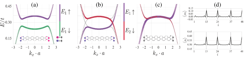
Figure 1: Dispersion relation of a Kramers pair of the different solutions to the mean-field problem for a $N=12$ ribbon computed for the single-orbital model. The bands are colored by edge ($E_{1}/E_{2}$) and real spin ($\uparrow/\downarrow$). The Kramers pairs can be obtained by TR symmetry. a) AFM phase b) FM phase c) The PHS broken non-magnetic phase with $\Delta N=1.92$. Lower inset in (a, b) depict the corresponding local magnetization or local additional occupation of (c). (d) Local magnetization $\langle m\rangle$ for the ground state of (a) and local density $\langle n\rangle$ corresponding to (c).

As it is habitual in self-consistent methods, the character of the converged solution reflects that of the initial guess. Breaking time-reversal (TR) symmetry by starting with parallel spin edges leads to a magnetic phase with a finite total spin-magnetic moment, whereas an initial state with polarized edges of opposite sign leads to a solution with broken spin rotations and zero total spin. In both cases, half-filling is imposed. Another possibility (although commonly ignored), is to consider TR-symmetric solutions with broken electron-hole symmetry, namely, a doped solution. This can be achieved by an initial state with an excess of holes or electrons, and usually converges to a non-magnetic phase. In what follows, we distinguish between magnetic and non-magnetic solutions. The former occurs at half-filling $\langle n_{i}\rangle=0.5$ whereas the latter has no local magnetization. The order parameter of this non-magnetic, PHS broken solution is given in terms of the local doping $\delta n_{i}$, giving the local occupation per spin of $\langle n_{i}\rangle=0.5+\delta n_{i}$, whereas the magnetic phase is characterized by a finite local magnetization $\langle m_{i}\rangle$.

We consider first a single-orbital ($p_{z}$) model in a nanoribbon with $N=12$ rows and $4$ columns, using $U=0.6t$. States with local ferrimagnetic spin polarization close to the edges have already been theoretically obtained Lado et al. (2015); Lado and Fernández-Rossier (2014a, b); Yazyev et al. (2011); Yazyev and Katsnelson (2008); Wan et al. (2011), where the edges may exhibit parallel (FM) or antiparallel (AFM) spin alignment with respect to each other. Fig. 1 contains the dispersion relation of the mid-bands, where bright color indicates edge-localized state. These bands are mainly located at the edges (E1, E2) of the sample, such that TR partners are localized at the opposite edge Wan et al. (2011). The AFM solution in (a) corresponds to a trivial insulator, with a gap arising from the broken rotational symmetry Son et al. (2006): From a symmetry perspective, the $E_{2}\uparrow$ state is degenerate with the $E_{1}\downarrow$ one and vice versa, but these states are not related by a rotation. From an interaction picture, the AFM exchange interaction acts as a staggered sublattice potential, which introduces a spin-dependent gap for states localized at different edges Kane and Mele (2005b); Ganguly et al. (2017). Fig. 1 (b) shows the FM solution, where two states with opposite spin cross the band gap. The coupling mechanism of states localized at two opposing edges can be described in analogy to the super exchange mechanism Jung et al. (2009); Kunstmann et al. (2011). From a topological standpoint, chiral symmetry is the reason for the occurrence of gap-crossing states Asbóth et al. of opposite Fermi velocity Veyrat et al. (2020), whereas from a group symmetry perspective, these solutions maintain invariance with respect to the two-fold axis, unlike the AFM case.

An additional phase is encountered in this work, namely, a non-magnetic PHS-broken solution, see Fig. 1 (c), where the additional $p_{z}$-orbital population shifts the Fermi energy above $U/2$. The electronic occupation is symmetrically distributed along the edges of the sample, maintaining the original $C_{2\nu}$ point group of the lattice. This results in a topologically non-trivial phase, just like in the non-interacting spin-Hall insulating case Kane and Mele (2005a). The corresponding order parameters are depicted in Fig. 1 (d), that is, the on-site magnetization $\langle m_{i}\rangle=\frac{1}{2}(\langle\hat{n}_{i,\uparrow}\rangle-\langle\hat{n}_{i,\downarrow}\rangle)$ for the magnetic phases and the occupation for the PHS-broken solution, $\langle n_{i}\rangle=\frac{1}{2}(\langle\hat{n}_{i,\uparrow}\rangle+\langle\hat{n}_{i,\downarrow}\rangle)$. Values are plotted as a function of the site index $i$ in sequence that follows columns (left to right) and rows (top to bottom) of the unit cell depicted in the insets of Fig. 1 (a-c). For the FM solution, the magnetization is largest at the edge sites, with an exponential decay towards the bulk. The AFM phase (not shown) has similar magnetization, only with opposite sign at each edge. The PHS broken solution lacks of magnetic moments, however, the electronic occupation off half filling shows a similar behavior as $\langle m\rangle$ in the magnetic solutions. We stress that a similar solution with negative occupation off half filling (or hole-doped) is also found when the initial state has a filling slightly below half filling.

It is worth mentioning that the topologically trivial AFM solution minimizes the free energy when the half-filling condition is imposed. However, dopants change this criterion and allows for a PHS broken state. In what follows we examine the free energy, the local magnetization and the occupation of these three solutions as a function of ribbon size and interaction parameters in single and multi-orbital approach.

III.2 Energetic considerations

Lieb’s theorem states that the ground state at half-filling has zero spin-magnetic moment Lieb (1989). It follows that the ground state at half-filling is always the AFM edge phase, regardless of ribbon size and for all $U>0$. However, Lieb’s theorem does not apply for doped systems, allowing for a ground state without any local spin-magnetic moment. We first compute and analyze the free energy of the three phases within the single-orbital model, and extend our computation to the multi-orbital model.

III.2.1 Single-orbital model

We first employ a single-orbital ($p_{z}$) model, where $t_{ij}=V_{pp\pi}\equiv t$ in Eq. (1), and with the Hubbard term being the only interacting term. We compute the free energy of the ground state for the different solutions. In Fig. 2 (a) the energy differences of the two magnetic phases at half-filling for three different ribbon sizes $N=8$, $12$ and $20$ is shown as a function of $U$, where the AFM phase is found to always be lower in energy. As expected, the energy separation between both phases increases with the interaction parameter $U$. For $N=8$, the reduced edge separation results in a relative lower energy of the AFM due to the inter-edge super exchange mechanism Jung et al. (2009). For larger $N$ this energy gain becomes smaller and a law $\sim N^{-2}$ can be seen in Fig. 2 (b) for both $U/t=0.6$ and $U/t=1$. Hence, it is to be expected that in the thermodynamic limit $N\to\infty$ both magnetic phases become equally probable, as $E_{\rm FM}-E_{\rm FM}\ll k_{B}T$.

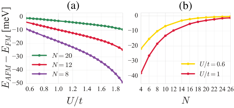
Figure 2: Energy differences of FM and AFM phases for (a) $N=8$, $12$ and $20$ as a function of $U$ and (b) for $U/t=0.6$ and $U/t=1$, as a function of number of rows $N$.

We consider next the PHS broken solutions, where the Stoner criterion justifies the absence of magnetism in doped systems, as an increase of the Fermi energy above the peak in the density of states removes the magnetic instability Fazekas ; Fernández-Rossier (8 02). We examine the behavior of the energy of the non-magnetic phase as the filling is shifted by an amount $\delta n$ off half-filling. Fig. 3 shows the free energy as a function of doping for a $N=8$ and $U=0.6$ nanoribbon. Here, the doping is expressed in cm^-2 units, $n=\delta n/S$ where $S=6.24\times 10^{-15}$cm² is the area of the ribbon. For low $\delta n$, the free energy obtained numerically has a quadratic dependency on the doping,

$$F(U,n) =UN\left(1+\frac{nS}{4N}\right)^{2},$$ (6)

which corresponds to the interacting term of Eq. (4). For larger doping, $|n|>250$ $\times 10^{12}$cm^-2, a stronger quadratic dependency on $n$ is observable. Here, the kinetic energy gain given by $H_{0}$ is larger than the effective reduction via Coulomb interaction, giving rise to a strong quadratic increase in energy. This results in a minimum for the free energy, which is encountered in the hole doping regime at the boundary between small and large filling.

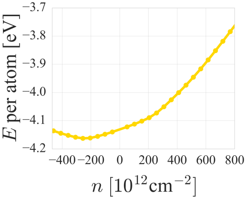
Figure 3: The energy of the PHS broken phase for different amounts of doping for $N=8$ and $U/t=0.6$ in the single-orbital model.

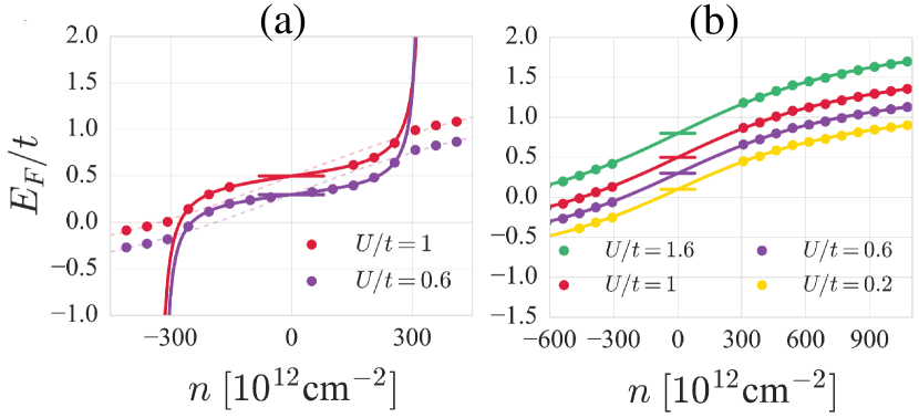
Figure 4: The Fermi energy of the PHS broken solution for $N=8$ and different $U/t$. The horizontal bar indicates the Fermi energy of the two magnetic phases at half-filling. a) For smaller doping the Fermi energy is fitted via $\tan{n}$. The dashed lines correspond to a fit via $\arctan{n}$. b) Fit with $\arctan{n}$ for larger doping, for four different Hubbard parameters: $U/T=$ 0.2, 0.6, 1.0 and 1.6.

Fig. 4 (a) shows the Fermi energy as a function of $U/t$, where the two doping regimes are visible. The separation between the small and large doping regimes occurs around $|n|\approx 250$ $\times 10^{12}$cm^-2. A function $\tan{n}$ fits very well to the data of the small doping regime, which is indicated in the figure by solid lines.

For larger doping, however, the Fermi energy has a different dependency, namely $\arctan{n}$, given by dashed lines in Fig. 4 (a). This dependency is still visible when $U/t$ is varied between $0.2$ and $1.6$ for dopings up to $n=10^{15}$cm^-2, as shown in Fig. 4 (b). While these results have been obtained in small systems, this behavior should scale to larger ribbons. The amount of doping at which the bulk states become filled in larger nanoribbons is reduced, as the band separation decreases with a power law Wakabayashi et al. (2010) of $\sim 1/N$ . This suggests that in larger graphene nanostructures, the doping required to reach the energetic minimum decreases, which may serve as an explanation to the elusive measurement of magnetic edges in graphene ribbons, which was previously unaccounted for.

III.2.2 Multi-orbital model

We consider next the multi-orbital model by including the $d_{xz}$- and $d_{yz}$-orbitals, which breaks PHS. We define $\delta n_{p}$ and $\delta n_{d}$ as the $p_{z}$- and $d$-orbital doping, respectively. The half-filling condition reads $\delta n_{p}=-\delta n_{d}$, where the orbital occupation per spin is given by $n_{p}=0.5+\delta n_{p}$ and $n_{d}=\delta n_{d}$, respectively. This leads to a renormalization of the orbital energies, namely:

$$E_{\alpha}(\delta n_{\alpha}) =\sum_{\sigma}\left[E_{d}+\delta n_{\alpha}\left(2V-J\right)\right]\hat{n}_{\alpha\sigma},$$ (7)

where we can infer that a decreased energetic separation of $p_{z}$ and $d$-orbitals lead to enhancement of the d-band population and vice-versa.

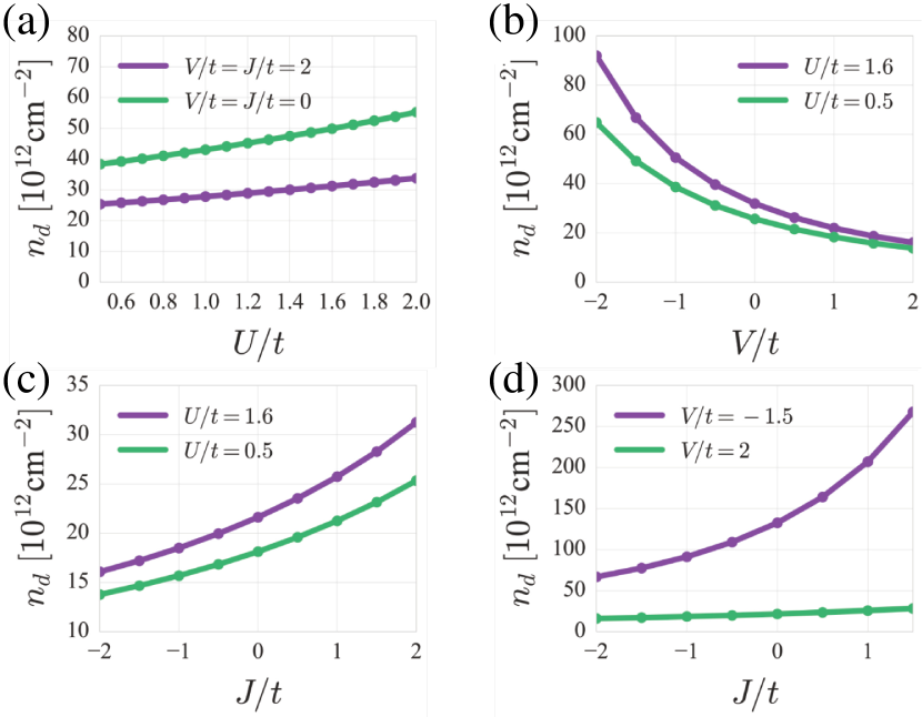
Figure 5: Total $d$-state occupation of a ribbon with $N=8$ plotted for different interacting parameters. Both FM and AFM phase have identical occupation.

Fig. 5 shows $n_{d}$ as a function of the interacting parameters in units of $t$. When $V$ and $J$ are kept constant, an increased $U$ leads to a larger occupation of the $d$-orbitals [see Fig. 5 (a)], as the Coulomb repulsive interaction is larger at the occupied $p_{z}$ orbitals. For negative $V$ or positive $J$, the $d$-orbital occupation becomes larger, as the $d$-orbital energy shift is reduced, as is shown in (b) and (c), respectively. Finally, Fig. 5 (d) shows that typical positive $V$ values yield small $d$-band occupation for any $J$, whereas negative $V$ results in $d$ population up to two orders of magnitude larger. We stress, however, that the repulsive (physical) Coulomb interaction yields $V,J>0$.

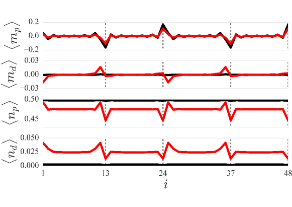
Figure 6: The expectation value of the magnetization $m_{p/d}$ and occupation $n_{p/d}$ per site and spin for a ribbon with $N=12$ in the AFM phase, where $U=1.6t$ and $J=0.5t$, with $V=-2t$ (red) and $V=2t$ (black).

Fig. 6 shows the local magnetization and orbital doping of a 48-sites ribbon in the AFM phase, with $U=1.6t$ and $J=0.5t$. An attractive $d$-orbital Coulomb interaction $V=-2t$ (red) results in an enhanced $d$-orbital magnetization at the sites next to the edge, whereas the single orbital results are recovered for a repulsive $d$-orbital Coulomb interaction $V=2t$ (black).

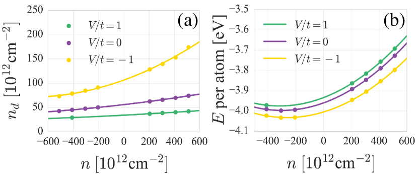
Figure 7: Results for a nanoribbon with $N=8$, for $U/t=1$ and $J/t=1$. a) Total $d$-state occupation and b) energy of the non-magnetic phase for different doping strengths $n$ for $V/t=1$, $0$ and $-1$.

Finally, we consider the multi-orbital doped solution. Fig. 7 (a) shows the $d$-orbital doping as a function of total doping, $n=(\delta n_{p}+\delta n_{d})/S$ for positive (green), zero (purple) and negative (yellow) $p$-$d$ Coulomb interaction, $V$. A quadratic law is observed for the latter, whereas a slow, linear increase in $d$-orbital occupation occurs for the former. The free-energy functional at low doping results now in:

$$F(n,U,V,J)=UN\left(1+\frac{\delta n_{p}}{4N}\right)^{2}+\left(2V-J\right)n_{p}\delta n_{d},$$ (8)

where $n_{p}=nS-\delta n_{d}$. The first term dominates, and was already observed in the single-orbital model [see Eq. (6)]. For larger dopings, the kinetic energy raises, and the single-orbital results are recovered, with the total minimum appearing for similar doping values. The inclusion of $d$-orbitals does not lead to qualitative differences for the free energy or the character of the ground state, compared to the single-orbital model. However, regarding the additional orbitals is imperative in low-energy considerations, such as the size of the intrinsic SOC band gap, which is linear with the $d$-orbital occupation Konschuh et al. (2010).

IV Conclusion

We have examined three different edge phases in terms of local magnetization and local orbital population, both in the single and in the multi-orbital model, of graphene nanoribbons with zigzag edges. For half-filling and finite interaction strengths the inter-edge super exchange mechanism predicts a lower free energy of the AFM phase compared to the FM phase. Our mean-field numerical calculations on graphene nanoribbons confirm these results. The PSH symmetry broken phase shows a minimum in the free energy at the boundary between the small and the large hole doping regime. In the former regime, the local doping occurs exclusively at the edge atoms, lowering the energy via exchange, whereas in the latter, the doping spreads throughout the bulk, lowering the kinetic energy and hence, increasing the free energy. These result are unchanged in a multi-orbital model and we have also briefly discussed the expected validity of our findings for larger systems. Thus, the multi-orbital computations confirm that the single-orbital description remains a good approximation for the energy gap of the two magnetic phases, whereas the $d$-orbital occupation only becomes relevant at attractive Coulomb interaction parameters. In the thermodynamic limit (large $N$, small interactions) the free energy of the three edge phases coincide, and hence, observation of a magnetic state would require very low temperatures, small ribbon sizes and specific low-interacting, acceptor substrates.

V Acknowledgements

This work is supported/funded by the Cluster of Excellence ”CUI: Advanced Imaging of Matter” of the Deutsche Forschungsgemeinschaft (DFG) – EXC 2056 – project ID 390715994. We thank A. Chudnovskiy and R. H. Blick for fruitful discussions.

References

- Fruchart and Carpentier (2013) M. Fruchart and D. Carpentier, Comptes Rendus Physique 14, 779 (2013).
- (2) J. K. Asbóth, L. Oroszlány, and A. Pályi, A Short Introduction to Topological Insulators (Springer International Publishing).
- Gosálbez-Martínez et al. (2012) D. Gosálbez-Martínez, D. Soriano, J. Palacios, and J. Fernández-Rossier, Solid State Communications 152 (2012), 10.1016/j.ssc.2012.04.046.
- Yazyev et al. (2011) O. V. Yazyev, R. B. Capaz, and S. G. Louie, Phys. Rev. B 84, 115406 (2011).
- Yazyev (2010) O. V. Yazyev, Reports on Progress in Physics 73, 056501 (2010).
- Yazyev and Katsnelson (2008) O. V. Yazyev and M. I. Katsnelson, Phys. Rev. Lett. 100, 047209 (2008).
- Wimmer et al. (2008) M. Wimmer, i. d. I. m. c. Adagideli, S. m. c. Berber, D. Tománek, and K. Richter, Phys. Rev. Lett. 100, 177207 (2008).
- Muñoz Rojas et al. (2009) F. Muñoz Rojas, J. Fernández-Rossier, and J. J. Palacios, Phys. Rev. Lett. 102, 136810 (2009).
- Friedrich et al. (2020) N. Friedrich, P. Brandimarte, J. Li, S. Saito, S. Yamaguchi, I. Pozo, D. Peña, T. Frederiksen, A. Garcia-Lekue, D. Sánchez-Portal, and J. I. Pascual, Phys. Rev. Lett. 125, 146801 (2020).
- Li et al. (2021) J. Li, S. Sanz, N. Merino-Díez, M. Vilas-Varela, A. Garcia-Lekue, M. Corso, D. G. de Oteyza, T. Frederiksen, D. Peña, and J. I. Pascual, “Topological phase transition in chiral graphene nanoribbons: from edge bands to end states,” (2021), arXiv:2103.15937 [cond-mat.mes-hall] .
- Kobayashi et al. (2005) Y. Kobayashi, K.-i. Fukui, T. Enoki, K. Kusakabe, and Y. Kaburagi, Physical Review B 71, 193406 (2005).
- Shibayama et al. (2000) Y. Shibayama, H. Sato, T. Enoki, and M. Endo, Physical Review Letters 84, 1744 (2000).
- Joly et al. (2010) V. L. J. Joly, M. Kiguchi, S.-J. Hao, K. Takai, T. Enoki, R. Sumii, K. Amemiya, H. Muramatsu, T. Hayashi, Y. A. Kim, M. Endo, J. Campos-Delgado, F. López-Urías, A. Botello-Méndez, H. Terrones, M. Terrones, and M. S. Dresselhaus, Physical Review B 81, 245428 (2010).
- Li et al. (2014) Y. Y. Li, M. X. Chen, M. Weinert, and L. Li, Nature Communications 5, 4311 (2014).
- Tao et al. (2011) C. Tao, L. Jiao, O. V. Yazyev, Y.-C. Chen, J. Feng, X. Zhang, R. B. Capaz, J. M. Tour, A. Zettl, S. G. Louie, H. Dai, and M. F. Crommie, Nature Physics 7, 616 (2011).
- Magda et al. (2014) G. Z. Magda, X. Jin, I. Hagymási, P. Vancsó, Z. Osváth, P. Nemes-Incze, C. Hwang, L. P. Biró, and L. Tapasztó, Nature 514, 608 (2014).
- Kane and Mele (2005a) C. L. Kane and E. J. Mele, Physical Review Letters 95, 226801 (2005a).
- Kane and Mele (2005b) C. L. Kane and E. J. Mele, Physical Review Letters 95, 146802 (2005b).
- Goldman et al. (2012) N. Goldman, W. Beugeling, and C. M. Smith, Europhysics Letters Association 97, 23003 (2012).
- Rachel (2018) S. Rachel, Reports on Progress in Physics 81, 116501 (2018).
- Zheng et al. (2011) D. Zheng, G.-M. Zhang, and C. Wu, Physical Review B 84, 205121 (2011).
- Hohenadler et al. (2014) M. Hohenadler, F. Parisen Toldin, I. F. Herbut, and F. F. Assaad, Physical Review B 90, 085146 (2014).
- Cao and Xiong (2013) J. Cao and S.-J. Xiong, Physical Review B 88, 085409 (2013).
- Luo (0 08) M. Luo, Physical Review B 102, 075421 (2020-08).
- Soriano and Fernández-Rossier (2010) D. Soriano and J. Fernández-Rossier, Physical Review B 82, 161302 (2010).
- Lado et al. (2015) J. Lado, N. García-Martínez, and J. Fernández-Rossier, Synthetic Metals 210, 56 (2015).
- Jung et al. (2009) J. Jung, T. Pereg-Barnea, and A. H. MacDonald, Physical Review Letters 102, 227205 (2009).
- Fernández-Rossier (8 02) J. Fernández-Rossier, Physical Review B 77, 075430 (2008-02).
- Wakabayashi et al. (1998) K. Wakabayashi, M. Sigrist, and M. Fujita, Journal of the Physical Society of Japan 67, 2089 (1998).
- Jung and MacDonald (2009) J. Jung and A. H. MacDonald, Physical Review B 79, 235433 (2009).
- Fan et al. (2012) X. F. Fan, W. T. Zheng, V. Chihaia, Z. X. Shen, and J.-L. Kuo, Journal of Physics: Condensed Matter 24, 305004 (2012).
- Varchon et al. (2007) F. Varchon, R. Feng, J. Hass, X. Li, B. N. Nguyen, C. Naud, P. Mallet, J.-Y. Veuillen, C. Berger, E. H. Conrad, and L. Magaud, Phys. Rev. Lett. 99, 126805 (2007).
- Henck et al. (2017) H. Henck, D. Pierucci, G. Fugallo, J. Avila, G. Cassabois, Y. J. Dappe, M. G. Silly, C. Chen, B. Gil, M. Gatti, F. Sottile, F. Sirotti, M. C. Asensio, and A. Ouerghi, Phys. Rev. B 95, 085410 (2017).
- Correa et al. (2018) J. H. Correa, A. Pezo, and M. S. Figueira, Physical Review B 98, 045419 (2018).
- Polini et al. (2008) M. Polini, A. Tomadin, R. Asgari, and A. H. MacDonald, Physical Review B 78, 115426 (2008).
- Feldner et al. (2010) H. Feldner, Z. Y. Meng, A. Honecker, D. Cabra, S. Wessel, and F. F. Assaad, Physical Review B 81, 115416 (2010).
- Konschuh et al. (2010) S. Konschuh, M. Gmitra, and J. Fabian, Physical Review B 82, 245412 (2010).
- Sichau et al. (2019) J. Sichau, M. Prada, T. Anlauf, T. J. Lyon, B. Bosnjak, and R. Tiemann, L. Blick, Physical Review Letters 122, 046403 (2019).
- Prada (2021) M. Prada, Phys. Rev. B 103, 115425 (2021).
- Prada et al. (2021) M. Prada, L. Tiemann, J. Sichau, and R. H. Blick, Phys. Rev. B 104, 075401 (2021).
- Slater and Koster (1954) J. C. Slater and G. F. Koster, Physical Review 94, 1498 (1954).
- Gosálbez-Martínez et al. (2011) D. Gosálbez-Martínez, J. J. Palacios, and J. Fernández-Rossier, Physical Review B 83, 115436 (2011).
- Pisani et al. (2007) L. Pisani, J. A. Chan, B. Montanari, and N. M. Harrison, Physical Review B 75, 064418 (2007).
- Kuroda and Shirakawa (1987) S.-i. Kuroda and H. Shirakawa, Physical Review B 35, 9380 (1987).
- Claveau et al. (2014) Y. Claveau, B. Arnaud, and S. D. Matteo, European Journal of Physics 35, 035023 (2014).
- Lado and Fernández-Rossier (2014a) J. L. Lado and J. Fernández-Rossier, Phys. Rev. Lett. 113, 027203 (2014a).
- Lado and Fernández-Rossier (2014b) J. L. Lado and J. Fernández-Rossier, Phys. Rev. B 90, 165429 (2014b).
- Wan et al. (2011) X. Wan, A. M. Turner, A. Vishwanath, and S. Y. Savrasov, Physical Review B 83, 205101 (2011).
- Son et al. (2006) Y.-W. Son, M. L. Cohen, and S. G. Louie, Physical Review Letters 97, 216803 (2006).
- Ganguly et al. (2017) S. Ganguly, M. Kabir, and T. Saha-Dasgupta, Physical Review B 95, 174419 (2017).
- Kunstmann et al. (2011) J. Kunstmann, C. Özdoğğan, A. Quandt, and H. Fehske, Physical Review B 83, 045414 (2011).
- Veyrat et al. (2020) L. Veyrat, C. Déprez, A. Coissard, X. Li, F. Gay, K. Watanabe, T. Taniguchi, Z. Han, B. A. Piot, H. Sellier, and B. Sacépé, Science 367, 781 (2020).
- Lieb (1989) E. H. Lieb, Physical Review Letters 62, 1201 (1989).
- (54) P. Fazekas, Lecture Notes on Electron Correlation and Magnetism, Series in Modern Condensed Matter Physics, Vol. 5 (World Scientific).
- Wakabayashi et al. (2010) K. Wakabayashi, K.-i. Sasaki, T. Nakanishi, and T. Enoki, Science and Technology of Advanced Materials 11, 054504 (2010).