One-loop structure of parton distribution for the gluon condensate and “zero modes”

Abstract

We present results for one-loop corrections to the recently introduced “gluon condensate” PDF $F(x)$. In particular, we give expression for the $gg$-part of its evolution kernel. To enforce strict compliance with the gauge invariance requirements, we have used on-shell states for external gluons, and have obtained identical results both in Feynman and light-cone gauges. No “zero mode” $\delta(x)$ terms were found for the twist-4 gluon PDF $F(x)$. However a $q^{2}\delta(x)$ term was found for the $\xi=0$ GPD $F(x,q^{2})$ at nonzero momentum transfer $q$. Overall, our results do not agree with the original attempt of one-loop calculations of $F(x)$ for gluon states, which sets alarm warning for calculations that use matrix elements with virtual external gluons and for lattice renormalization procedures based on their results.

1 Introduction

The use of parton distribution functions (PDFs) $f(x)$ Feynman:1973xc is an important tool to accumulate information about hadron structure. For many decades, PDFs were the objects of intensive experimental studies, and now also of lattice QCD calculations as well. The gluon PDFs are the most difficult to investigate, both experimentally and on the lattice. The “classic” gluon PDFs, unpolarized and polarized ones, are both related to twist-2 operators built from the gluon fields. Recently, X. Ji proposed Ji:2020baz to consider gluon PDFs generated from the twist-4 operators of $G^{+-}\ldots G^{+-}$, etc. type. In Ref. Hatta:2020iin , the twist-4 PDF $F(x)$ corresponding to the $G_{\mu\nu}\ldots G^{\mu\nu}$ operators was introduced. Its importance stems from the fact that the matrix element of the local operator $\langle P|G_{\mu\nu}(0)G^{\mu\nu}(0)|P\rangle$ may be related to the gluon contribution into the proton mass.

An interesting question is whether $F(x)$ has a singular $\delta(x)$ part, sometimes dubbed as a “zero-mode” contribution. Such terms have been observed Burkardt:2001iy in one-loop perturbative QCD expressions for the twist-3 quark PDFs. The presence of such terms in twist-4 gluon PDFs was suggested in Ref. Ji:2020baz . For $F(x)$, this question was addressed in Ref. Hatta:2020iin through a one-loop calculation of the matrix element of the bilocal operator $G_{\mu\nu}(z)G^{\mu\nu}(0)$ between virtual gluon states.

The calculation of Ref. Hatta:2020iin was performed in the light-cone gauge $(nA)=0$ and produced a $1/x$ term in the evolution kernel. It has emerged from the $1/(kn)$ factor of the gluon propagator in the light-cone gauge. The authors of Ref. Hatta:2020iin assumed that this $1/(kn)$ singularity should be supplied by the Mandelstam-Leibbrandt prescription Leibbrandt:1987qv which converts $1/x$ into $(1/x)_{+}$. Formally, the “plus” prescription for $1/x$ contains the $\delta(x)$ term, and one may argue that this is an indication for “zero-mode” terms in $F(x)$. However, the $x$-integral of $(1/x)_{+}$ vanishes, while the genuine “zero-mode” terms, like those observed in Ref. Burkardt:2001iy , are expected to have a pure $\delta(x)$ form that gives a nonzero contribution after integration.

A more essential question is whether this $1/x$ term exists at all. A worrisome fact is that the calculation of Ref. Hatta:2020iin was done using external gluons with nonzero virtuality, which violates gauge invariance. A natural check would be to calculate the same matrix element using another gauge, which has not been done in Ref. Hatta:2020iin . So, we did such a calculation using Feynman gauge and obtained a completely different result. In particular, its evolution kernel part does not have the $1/x$ term found in the light-cone-gauge calculation, but contains a familiar/expected $\sim[1/(1-x)]_{+}$ bremsstrahlung term absent in the result of Ref. Hatta:2020iin .

Our goal in the present paper is to revisit the issue of one-loop corrections for $F(x)$, and perform their calculation in a gauge-invariant way.

To secure gauge invariance, one needs to do the calculations using on-shell external gluons. However, the tree-level matrix element of the $G_{\mu\nu}(0)G^{\mu\nu}(z)$ operator for such states vanishes. To avoid this problem, we have proposed to take a nonforward matrix element between on-shell gluons with different lightlike momenta $p_{1}$ and $p_{2}=p_{1}+q$. In other words, we have considered the generalized parton distribution (GPD) $F(x,\xi,q^{2})$ corresponding to the same bilocal operator $G_{\mu\nu}(0)G^{\mu\nu}(z)$ as in Eq. (1).

We have found that the $\xi=0$ GPD $F(x,q^{2})$ contains a $\delta(x)$ term. However, it is accompanied by a $q^{2}$ factor and vanishes in the $q\to 0$ limit, so that the “forward” PDF $F(x)$ does not have $\delta(x)$ terms at one loop. We have also obtained the one-loop evolution kernel for $F(x)$ and observed that it is given by a $\sim[1/(1-x)]_{+}$ bremsstrahlung term and nothing else. No $1/x$ singularities in the evolution kernel have been detected.

The paper is organized in the following way. We start, in Section 2, with the description of results obtained using off-shell gluons. In Section 3, we introduce the GPD corresponding to a nonforward matrix element for on-shell gluons. In Section 4, we present our results for the main bulk of diagrams, the “real corrections”, and show that, for nonzero $q^{2}$, they contain the “zero mode” $\delta(x)$ term. The formal origin of the $\delta(x)$ terms in one-loop integrals is investigated in Section 5. The structure of singularity at the $x=\pm 1$ endpoints is studied in Section 6. We separate this singularity into a term that is regularized by the plus-prescription at $x=1$, and a term proportional to $\delta(1-x)$. In Section 7, we investigate its structure and discuss taking the $q^{2}\to 0$ limit. Finally, in Section 8 we summarize the paper and formulate our conclusions.

2 Regularization by external gluon virtuality

The twist-4 PDF $F(x)$ may be defined Hatta:2020iin through a bilocal operator $G_{\mu\nu}(0)W[0,z]G^{\mu\nu}(z)$ on the light cone $z^{2}=0$

$$F(x)=\frac{P^{+}}{2M^{2}N_{g}}\int\frac{dz^{-}}{2\pi}e^{ixP^{+}z^{-}}\left\langle P\left|G^{a}_{\mu\nu}(0)W[0,z^{-}]G_{a}^{\mu\nu}\left(z^{-}\right)\right|P\right\rangle\ ,$$

where $W[0,z]$ is the usual gauge link, $N_{g}=N_{c}^{2}-1$ is the number of gluons, and summation over the hadron polarizations is implied. The “plus”-components are obtained by a scalar product with a light-cone vector $n$, i.e., for an arbitrary vector $a$, one has $n\cdot a=a^{+}.$

In this definition of $F(x)$, it is assumed that there is no gluon propagator between the field points $-z^{-}/2$ and $z^{-}/2$, i.e. the $G$-fields enter through a normal product. Also, it is implied that the $GG$ bilocal operator is in a $T$-product with the $S$-matrix, i.e. one deals with an “uncut” PDF. This means that, in perturbation theory, all the diagram lines correspond to usual propagators. For this reason, the “uncut” PDFs have the canonical support $|x|\leq 1$ (see, e.g., Ref. Radyushkin:1983wh for an all-order proof). Furthermore, the only foreseeable way to extract these twist-4 PDFs is through lattice simulations, and lattice calculations, of course, involve just uncut propagators.

The starting point of perturbative calculations is a tree diagram corresponding to the matrix element of the twist-4 gluon operator between gluon states with equal momentum $p$. For further generalizations, we take different polarizations $\epsilon_{1},\epsilon_{2}^{*}$ for these lines. At the tree-level, we have

$$\frac{p^{+}}{N_{g}} \int\frac{dz^{-}}{2\pi}e^{ixp^{+}z^{-}}\left\langle g\left(p,\epsilon_{2}^{*}\right)\left|G^{a}_{\mu\nu}(0)W[0,z]G_{a}^{\mu\nu}\left(z^{-}\right)\right|g\left(p,\epsilon_{1}\right)\right\rangle^{(0)}$$

$$= n\cdot p\left(p^{\mu}\epsilon_{1}^{\nu}-p^{\nu}\epsilon_{1}^{\mu}\right)\left(p^{\mu}\epsilon_{2}^{*\nu}-p^{\nu}\epsilon_{2}^{*\mu}\right)\delta(n\cdot p-xn\cdot p)+\{x\to-x\}$$

$$=2\left(p^{2}\epsilon_{1}\cdot\epsilon_{2}^{*}-p\cdot\epsilon_{1}\,p\cdot\epsilon_{2}^{*}\right)\delta(1-x)+\{x\to-x\}\ .$$ (1)

One can see that, for on-shell gluons, i.e., when $p^{2}=0$ and $p\cdot\epsilon_{1}=p\cdot\epsilon_{2}=0$, the tree-level result vanishes. A non-vanishing result may be obtained if one takes off-shell gluons with $p^{2}\neq 0$. This has been done, in particular, by the authors of Ref. Hatta:2020iin . Such a choice has a certain risk, since the one-loop result may be not gauge invariant, especially given the fact that the tree-level expression (1) is proportional to $p^{2}$, the parameter characterizing the gauge invariance violation.

For one-loop calculations, one should specify the gauge. In general, the gluon propagator is $-iD^{\mu\nu}(k)/k^{2}$, where $D^{\mu\nu}(k)=g^{\mu\nu}$ in Feynman gauge and

$$D^{\mu\nu}(k)=g^{\mu\nu}-\frac{k^{\mu}n^{\nu}+k^{\nu}n^{\mu}}{n\cdot k}$$

in the light-cone gauge. Using the latter, and the dimensional regularization (DR) with $D=4-2\epsilon$, a one loop calculation was performed in Ref. Hatta:2020iin . As we will discuss later, the result has some peculiar features, so, for a check, we redid this calculation and obtained

$$F^{\rm LC}(x,p^{2})\bigg{|}_{(a+b+b^{\prime})} =-iC_{A}g^{2}\frac{p^{+}}{-p^{2}}\int\frac{dk^{-}d^{D-2}\vec{k}_{\perp}}{(2\pi)^{D}}$$

$$\times\frac{(1-\epsilon)(1-x)[2k^{-}p^{+}(4-5x)+p^{2}x(1+x)]+\vec{k}_{\perp}^{2}[4(1-\epsilon)+x(6\epsilon-4)]}{(1-\epsilon)x(1-x)[\vec{k}_{\perp}^{2}-(1-x)(p^{2}-2k^{-}p^{+})](\vec{k}_{\perp}^{2}-2k^{-}p^{+}x)}$$

$$+(x\to-x)$$ (2)

for the sum of diagrams $a)$, $b)$, $b^{\prime})$ of Fig. 1. This result coincides with Eq. (45) of Ref. Hatta:2020iin if one expresses there the denominators in the light-cone components and substitutes $k^{+}$ with $xp^{+}$. Taking the integrals and expanding in $\epsilon$ gives

$$F^{\rm LC}(x,p^{2})\bigg{|}_{(a+b+b^{\prime})} =-\frac{\alpha_{s}}{2\pi}C_{A}\bigg{\{}\bigg{[}\frac{1}{\epsilon}+\ln\frac{\mu^{2}}{-p^{2}x(1-x)}\bigg{]}\left(\frac{2}{x}-2+x\right)+x\bigg{\}}\ \theta(0<x<1)$$

$$+(x\to-x)\ .$$ (3)

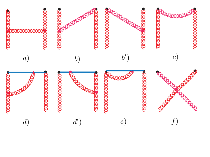
Figure 1: “Real” diagrams (mirror diagram $e^{\prime}$ is not shown).

The term $\sim 1/x$, singular for $x=0$, comes from the light-cone-gauge denominator factor $1/(kn)$ which, surprizingly, is not cancelled by numerator factors in this calculation. It is argued in Ref. Hatta:2020iin that one should use here the Mandelstam-Leibbrandt prescription Leibbrandt:1987qv for the $1/(kn)$ factor, which converts $1/x$ into $(1/x)_{+}$. The “plus” prescription for $1/x$ formally contains a $\delta(x)$ term. A minor comment here is that the $x$-integral of $(1/x)_{+}$ vanishes, which is not what is usually expected from the “zero-mode” terms. The latter are believed to have a pure $\delta(x)$ form for $x\sim 0$ that integrates to a nonzero contribution. Another strange feature of Eq. (3) is the absence of a $1/(1-x)$ bremsstrahlung contribution, typical for PDFs in gauge theories like QCD.

To check if it is worth efforts to investigate the puzzling structure of Eq. (3) any further, we have calculated $F(x)$ in Feynman gauge using, again, virtual external gluons. We found that the result is given by a completely different analytic expression. In particular, for terms containing the evolution logarithm $\ln(-\mu^{2}/p^{2})$, we have obtained

$$F^{\rm F}(x)\bigg{|}_{(a+b+b^{\prime}+d+d^{\prime})} =\frac{\alpha_{s}}{4\pi}C_{A}\bigg{\{}\bigg{[}\frac{1}{\epsilon}+\ln\frac{\mu^{2}}{-p^{2}x(1-x)}\bigg{]}\left(\frac{2}{1-x}+1-x\right)-\frac{1+2x^{2}}{x}\bigg{\}}$$

$$\times\theta(0<x<1)+(x\to-x)\ .$$ (4)

As one can observe, the evolution term here does not have a $1/x$ singularity for small $x$. However, it has the usual $1/(1-x)$ soft radiation singularity for $x=1$ absent in Eq.(3). Still, in Eq. (4), we see a $1/x$ term in the non-evolution part, with no evident prescription now how to regularize it.

The drastic difference between the Feynman- and light-cone-gauge results suggests that there are good chances that neither of them should be relied upon. A natural suspect for the origin of the discrepancy between the two results and of their peculiar features is the violation of gauge invariance stemming from using virtual external gluons.

3 Regularization by nonforward kinematics for on-shell gluons

To get a nonzero result at the tree level, and preserve gauge invariance at the one-loop level, we have decided to take on-shell gluons, but impose a nonzero momentum transfer between them. This means that we consider the generalized parton distribution (GPD). The non-forward matrix element defining this GPD is given by

$$F\left(x,p_{1},p_{2};\epsilon_{1},\epsilon_{2}\right) =\frac{P^{+}}{N_{g}}\int\frac{dz^{-}}{2\pi}e^{ixP^{+}z^{-}}$$

$$\times\left\langle g\left(p_{2},\epsilon_{2}\right)\left|G^{a}_{\mu\nu}\left(-\frac{z^{-}}{2}\right)W\left[-\frac{z}{2},\frac{z}{2}\right]G_{a}^{\mu\nu}\left(\frac{z^{-}}{2}\right)\right|g\left(p_{1},\epsilon_{1}\right)\right\rangle\ ,$$ (5)

where $p_{1}$ and $p_{2}$ are the on-shell ($p_{1}^{2}=p_{2}^{2}=0$) gluon momenta, $P=(p_{1}+p_{2})/2$ being their average, and $q=p_{2}-p_{1}$ being their difference. The skewness variable $\xi$ is defined using $p_{1}^{+}=(1+\xi)P^{+}$ and $p_{2}^{+}=(1-\xi)P^{+}$, so that $\xi=-{q^{+}}/{2P^{+}}.$ The gluon polarizations satisfy the usual relation for on-shell gluons $\quad p_{1}\cdot\epsilon_{1}=0,\quad p_{2}\cdot\epsilon_{2}^{*}=0$   .

With these definitions, we obtain the following tree-level result (recall $P^{+}=n\cdot P$, etc.)

$$F^{(0)}\left(x,p_{1},p_{2};\epsilon_{1},\epsilon_{2}\right) =n\cdot P\left(p_{1}^{\mu}\epsilon_{1}^{\nu}-p_{1}^{\beta}\epsilon_{1}^{\alpha}\right)\left(p_{2}^{\mu}\epsilon_{2}^{*\nu}-p_{2}^{\nu}\epsilon_{2}^{*\mu}\right)$$

$$\times[\delta(n\cdot P-x\,n\cdot P)+\delta(n\cdot P+x\,n\cdot P)]$$

$$=2\left(p_{1}\cdot p_{2}\,\epsilon_{1}\cdot\epsilon_{2}^{*}-p_{1}\cdot\epsilon_{2}^{*}\,p_{2}\cdot\epsilon_{1}\right)[\delta(1-x)+\delta(1+x)]$$

$$=\left(-q^{2}\epsilon_{1}\cdot\epsilon_{2}^{*}+2\,q\cdot\epsilon_{1}\,q\cdot\epsilon_{2}^{*}\,\right)[\delta(1-x)+\delta(1+x)]$$

$$\equiv\Pi(q,\epsilon_{1},\epsilon_{2})[\delta(1-x)+\delta(1+x)]\ .$$ (6)

We have used here that $p_{2}\cdot\epsilon_{1}=q\cdot\epsilon_{1}$ and $p_{1}\cdot\epsilon_{2}^{*}=-q\cdot\epsilon_{2}^{*}$, to make it explicit that the structure $\Pi(q,\epsilon_{1},\epsilon_{2})$ (and, hence, $F^{(0)}\left(x,p_{1},p_{2};\epsilon_{1},\epsilon_{2}\right)$) vanishes in the forward limit $q=0$.

In the nonforward case, we parametrize $F\left(x,p_{1},p_{2};\epsilon_{1},\epsilon_{2}\right)$ by two invariant functions

$$F\left(x,p_{1},p_{2};\epsilon_{1},\epsilon_{2}\right)= \epsilon_{1}^{\ \mu}\epsilon_{2}^{*\,\nu}\left[\left(2\,q_{\mu}q_{\nu}-q^{2}g_{\mu\nu}\right)F_{1}(x,\xi,q^{2})+g_{\mu\nu}F_{2}(x,\xi,q^{2})\right]$$

$$\equiv\Pi(q,\epsilon_{1},\epsilon_{2})F_{1}(x,\xi,q^{2})+\epsilon_{1}\cdot\epsilon_{2}^{*}F_{2}(x,\xi,q^{2})\ .$$ (7)

The Lorentz structure of the first term coincides with that observed at the tree level. It is produced by a traceless 2-dimensional tensor when $\alpha,\beta$ are chosen to be in the transverse plane. The second term corresponds to the trace in such 2-dimensional indices. Thus, at the tree level, we have $F_{1}^{(0)}(x,\xi,q^{2})=\delta(1-x)+\delta(1+x)$ and $F_{2}^{(0)}(x,\xi,q^{2})=0$.

4 Total result for “real corrections”

We have calculated the diagrams $1a)-1f)$ (sometimes called “real corrections”) both in Feynman and light-cone gauges (the details of these rather lengthy calculations will be presented in a separate paper Zhao ). In both gauges, we have obtained the same total expression.

Let us discuss first the results for $F_{1,2}^{(1)}(x,\xi,q^{2})$ away from the potentially singular endpoints $x=\pm 1$. We start with the function $F_{1}\left(x,\xi,q^{2}\right)$ that was nonzero at the tree level. At one loop, it has the following form

$$F_{1}^{(1)}\left(x,\xi,q^{2}\right) \left.\right|_{x\neq\pm 1}=\frac{\alpha_{s}}{\pi}C_{A}\frac{1}{1-x}\left\{\left(\frac{1}{\epsilon_{\rm UV}}+\ln\frac{\mu_{\rm UV}^{2}\left(1-\xi^{2}\right)}{-q^{2}(1-x)^{2}}\right)\theta(\xi<x<1)\right.$$

$$\left.+\frac{1}{2}\left(\frac{1}{\epsilon_{\rm UV}}+\ln\frac{\mu_{\rm UV}^{2}(\xi-x)(1+\xi)^{2}}{-q^{2}(1-x)^{2}(x+\xi)}\right)\theta(-\xi<x<\xi)\right\}+\{x\to-x\}\ .$$ (8)

As expected, it contains the evolution contribution revealed by the $1/\epsilon_{\rm UV}$ pole and the logarithmic $\ln(-\mu_{\rm UV}^{2}/q^{2})$ dependence on the UV regulator scale $\mu_{\rm UV}$.

One can see that the momentum transfer $q^{2}$ serves here as an IR cut-off, a subtlety that we will briefly address now and in more detail later on. The point is that, at intermediate stages of the calculations, we also had the integrals diverging both on UV and and IR sides and resulting in the poles $1/\epsilon_{\rm UV}-1/\epsilon_{\rm IR}$ and logarithms of $\ln(\mu^{2}_{\rm UV}/\mu^{2}_{\rm IR})$ type. However, all the poles $1/\epsilon_{\rm IR}$ and the dependence on $\mu_{\rm IR}$ cancel in the final result. A similar observation was made in the studies of the quark GPDs Liu:2019urm (see also Ji:2015qla ).

Since we are interested in the “forward” PDFs, we take the $\xi\to 0$ limit, to get

$$\left.F_{1}^{(1)}\left(x,q^{2}\right)\right|_{x\neq\pm 1}=\frac{\alpha_{s}}{\pi}C_{A} \left\{\frac{\theta(0\leq x<1)}{1-x}\left(\frac{1}{\epsilon_{\mathrm{UV}}}+\ln\frac{\mu_{\mathrm{UV}}^{2}}{-q^{2}(1-x)^{2}}\right)\right\}$$

$$+\{x\to-x\}\ .$$ (9)

Here and in what follows, we denote $F\left(x,\xi=0,q^{2}\right)=F\left(x,q^{2}\right)$ (similarly, we will denote later $F\left(x,q^{2}=0\right)=F\left(x\right)$).

Recall that the function $F_{2}\left(x,\xi,q^{2}\right)$ vanishes at the tree level. Thus, one would expect that it should not contain evolution logarithms at one loop. This expectation is supported by the actual one-loop result

$$F_{2}^{(1)}\left(x,\xi,q^{2}\right)=\frac{\alpha_{s}}{\pi}C_{A} q^{2}\left\{\frac{1-x}{1-\xi^{2}}\theta(\xi<x\leq 1)-\frac{1-\xi}{4\xi(1+\xi)}\theta(-\xi<x<\xi)\right\}$$

$$+\{x\to-x\}\ .$$ (10)

We have dropped here the $x\neq\pm 1$ restriction because $F_{2}^{(1)}\left(x,\xi,q^{2}\right)$ is not singular (in fact, vanishes) for $x=\pm 1$. Taking the $\xi\to 0$ limit of this expression is not straightforward, because it has a singular $\sim 1/\xi$ behavior in the central region $-\xi<x<\xi$. As one can notice, $\theta(-\xi<x<\xi)/2\xi$ converts into a “zero mode” $\delta(x)$ term in the $\xi\to 0$ limit. Using this observation and taking the $\xi\to 0$ limit, we get

$$F_{2}^{(1)}\left(x,q^{2}\right)= \frac{\alpha_{s}}{\pi}C_{A}q^{2}\left\{(1-x)\theta(0\leq x\leq 1)-\frac{1}{2}\delta(x)\right\}+\{x\to-x\}\ .$$ (11)

Clearly, the kinematics with $\xi=0$ may still be non-forward, as far as $q^{2}\neq 0$. Thus, one can try to calculate $F_{1,2}(x,q^{2})$ imposing the $\xi=0$ condition from the start. We did such a calculation, both in the light-cone and Feynman gauges. At the end, we have obtained identical total results coinciding with Eqs. (9), (11). In fact, such an outcome is not completely trivial, since we have observed that the results obtained from the $\xi\to 0$ limit of the $\xi\neq 0$ calculation sometimes differ on the diagram-by-diagram level from those obtained when $\xi$ equals zero from the beginning. Only the combined results coincide.

Thus, the only singularity for $x=0$ in the one-loop results (9), (11) is the $\delta(x)$ term in $F_{2}\left(x,q^{2}\right)$. All the other terms are not singular for $x=0$. Note, however, that the function $F_{2}^{(1)}\left(x,q^{2}\right)$ vanishes in the forward limit, when $q=0$. Thus, our perturbative one-loop calculation does not indicate presence of the “zero-mode” terms in the forward PDF $F(x)$. Still, one may say that the “zero-mode” $\delta(x)$ term is present for the $\xi=0$ GPD in the $F_{2}^{(1)}\left(x,q^{2}\right)$ term when $q^{2}\neq 0$. As a side remark, we note also that the $x$-integral of $F_{2}^{(1)}\left(x,q^{2}\right)$ vanishes.

5 “Zero modes” in one-loop integrals

A frequent argument for “zero modes”, i.e., $\delta(x)$ terms in parton distributions, is based on the results of perturbative one-loop calculations Burkardt:2001iy ; Aslan:2018tff ; Bhattacharya:2020jfj . It is interesting to trace the mechanism that leads to the $\delta(x)$ terms in the contributions of particular diagrams.

In our case, the “zero mode” terms in $F(x,q^{2})$ have been produced, in particular, by the box diagram $1a)$. Consider a generic one-loop integral corresponding to a box diagram in GPD kinematics, given by

$$I_{n_{1}n_{2}n_{3}}(x,\xi,q^{2})\sim\int d^{D}k\frac{P(k,p_{1},p_{2})}{(p_{1}-k)^{2n_{1}}k^{2n_{2}}(p_{2}-k)^{2n_{3}}}\delta(1-x-k^{+}/P^{+})\ ,$$ (12)

where the function $P(k,p_{1},p_{2})$ comes from numerator factors. “Zero modes” appear when $P(k,p_{1},p_{2})$ is proportional to $k^{2n_{2}}$, which cancels the middle propagator factor $1/k^{2n_{2}}$. The resulting integral does not depend on the virtualities of external momenta $p_{1}^{2},p_{2}^{2}$. Only the dependence on $q^{2}=(p_{2}-p_{1})^{2}$ (and $\xi$) remains. Take the simplest case when $n_{1}=n_{3}=1$, $n_{2}=0$ and $P(k,p_{1},p_{2})=1$, which we denote as $S_{101}$,

$$S_{101}(x,\xi,q^{2})\sim\int d^{D}k\frac{\delta(1-x-k^{+}/P^{+})}{(p_{1}-k)^{2}(p_{2}-k)^{2}}\ .$$ (13)

Writing the denominator factors in the Schwinger $\alpha$-representation, we have, in the $\overline{\rm MS}$ scheme,

$$S_{101}(x,\xi,q^{2})=(\mu^{2}e^{\gamma_{E}})^{\epsilon}\int_{0}^{\infty}\frac{d\alpha_{1}d\alpha_{3}}{(\alpha_{1}+\alpha_{3})^{2-\epsilon}}\delta\left(x-\frac{\xi(\alpha_{3}-\alpha_{1})}{\alpha_{1}+\alpha_{3}}\right)e^{q^{2}\alpha_{1}\alpha_{3}/(\alpha_{1}+\alpha_{3})}\ \ .$$ (14)

Rescaling $\lambda=(\alpha_{1}+\alpha_{3})\ ,\ \beta=\alpha_{1}/(\alpha_{1}+\alpha_{3})$ gives

$$S_{101}(x,\xi,q^{2})=(\mu^{2}e^{\gamma_{E}})^{\epsilon}\int_{0}^{\infty}\frac{d\lambda}{\lambda^{1-\epsilon}}\int_{0}^{1}d\beta\,\delta\left(x-\xi(1-2\beta)\right)e^{q^{2}\lambda\beta(1-\beta)}\ .$$ (15)

Since $|1-2\beta|\leq 1$, this contribution vanishes for $|x|>\xi$, so it exists in the middle region $|x|<\xi$ only (similar results have been obtained in calculations of twist-3 quark GPDs Aslan:2018tff ),

$$S_{101}(x,\xi,q^{2})=\frac{\theta(|x|<\xi)}{2\xi}(\mu^{2}e^{\gamma_{E}})^{\epsilon}\int_{0}^{\infty}\frac{d\lambda}{\lambda^{1-\epsilon}}e^{\lambda q^{2}(1-x^{2}/\xi^{2})/4}\to\frac{\theta(|x|<\xi)}{2\xi}\ln(-q^{2}/\mu^{2})+\ldots\ \ .$$ (16)

Taking the $\xi\to 0$ limit of $\theta(|x|<\xi)/2\xi$ gives $\delta(x)$, so $I_{101}(x,q^{2})\sim\delta(x)\ln(-q^{2}/\mu^{2})+\ldots$ . This result may also be obtained by simply substituting $\xi=0$ in Eq. (14). Note that the non-regularized $\lambda$-integral diverges in the region of small $\lambda$, i.e. in the UV region. Hence the $\mu$-parameter here has the meaning of $\mu_{\rm UV}$, with $-q^{2}$ serving as the IR cut-off in the large-$\lambda$ region.

The “zero mode” terms in $F(x,q^{2})$ may be produced also by the four-gluon-vertex diagram $1f)$. In this case, the $1/k^{2}$ propagator is absent from the beginning. In the light-cone gauge, we found that the “zero mode” terms $\delta(x)$ accompanied by $\ln(-q^{2}/\mu^{2})$ factors are present in $F_{1}(x,q^{2})$ for diagrams $1a)$ and $1f)$, but they cancel each other. The surviving “zero mode” term in $F_{2}(x,q^{2})$ has resulted from the diagram $1f)$. It comes from the integral (16) multiplied by an extra $\epsilon$ factor, which cancels the $1/\epsilon$ singularity produced by the integral over $\lambda$. In addition, there is a numerator $q^{2}$ factor accompanying this integral, which results in the $\sim q^{2}$ overall factor for the “zero mode” contribution to $F_{2}(x,q^{2})$.

6 Structure of singularity at $x=1$

Another domain, where one may expect singularities in QCD, is the soft-gluon region $x\sim 1$ (or $x\sim-1$), in which the external momentum is wholly carried by the active parton. Since the function $F(x,q^{2})$ is even in $x$, it is sufficient to discuss its $x\geq 0$ part.

In our case, the function $F_{1}^{(1)}\left(x,q^{2}\right)$ in Eq. (9) has a $1/(1-x)$ singularity in its evolution kernel. In the lightcone gauge, it comes solely from Fig. $1a)$, which produces the $1/(1-x)$ singularity in a “bare” form, without a plus-prescription for it, while the accompanying $\delta(1-x)$ terms come from self-energy diagrams.

In Feynman gauge, the diagram $1a)$ also produces $\sim 1/(1-x)$ terms, but they come, in addition, from the diagrams $1d)$ and $1d^{\prime}$) as well. These diagrams contain a gluon insertion into the gauge-link line. They produce equal contributions which, in fact, have the plus-prescription form for the singularity at $x=1$. Their sum is given by

$$F^{F}_{(1d+1d^{\prime})}\left(x,q,\epsilon_{1},\epsilon_{2}\right)= \frac{\alpha_{s}}{2\pi}C_{A}\left(\frac{1}{\epsilon_{\mathrm{UV}}}-\frac{1}{\epsilon_{\mathrm{IR}}}+\ln\frac{\mu_{\mathrm{UV}}^{2}}{\mu_{\mathrm{IR}}^{2}}\right)\Pi(q,\epsilon_{1},\epsilon_{2})\left[\theta(0\leq x\leq 1)\frac{x+x^{2}}{1-x}\right]_{+}$$

$$+\{x\to-x\}\ .$$ (17)

Note that the momentum integrals in these diagrams do not depend on the momentum transfer $q$, and diverge both at the UV and IR ends of integration, the fact reflected in the overall factor containing the poles.

The box diagram $1a)$ in Feynman gauge

$$F^{F}_{(1a)}(x,q,\epsilon_{1},\epsilon_{2})= \frac{\alpha_{s}}{2\pi}C_{A}\bigg{\{}\Pi(q,\epsilon_{1},\epsilon_{2})\bigg{[}(2+x)\left(\frac{1}{\epsilon_{\mathrm{UV}}}-\frac{1}{\epsilon_{\mathrm{IR}}}+\ln\frac{\mu_{\mathrm{UV}}^{2}}{\mu_{\mathrm{IR}}^{2}}\right)$$

$$-\frac{\Gamma(-\epsilon_{\mathrm{IR}})^{2}\Gamma(1+\epsilon_{\mathrm{IR}})}{\Gamma(-2\epsilon_{\mathrm{IR}})}\left(\frac{\mu_{\mathrm{IR}}^{2}e^{\gamma_{E}}}{-q^{2}}\right)^{\epsilon_{\mathrm{IR}}}(1-x)^{-1-2\epsilon_{\mathrm{IR}}}\bigg{]}$$

$$+2q^{2}\epsilon_{1}\cdot\epsilon_{2}^{*}(1-x)\bigg{\}}\theta(0<x\leq 1)+\{x\to-x\}+\delta(x)\ {\rm terms}\ ,$$ (18)

in its $\Pi(q,\epsilon_{1},\epsilon_{2})$ part, has two types of contributions for nonzero $x$. The first of them has the structure similar to those of diagrams $1d)$ and $1d^{\prime})$ , i.e., has both UV and IR poles.

Contributions of the second type are UV finite and have IR poles only. They are contained in the term with the gamma-functions in the second line of Eq.(18). This term corresponds to the basic integral (12) with $n_{1}=n_{2}=n_{3}=1$ and $P(k,p_{1},p_{2})=-q^{2}$. We denote it as $(-q^{2})S_{111}(x,q^{2})$. This integral is UV finite, but has collinear divergences due to vanishing virtualities $p_{1}^{2}=0$ and $p_{2}^{2}=0$ of external lines. To regularize these divergences, we have applied dimensional regularization in the $\overline{\rm MS}$ scheme. Using Schwinger representation, the regularized $S_{111}(x,q^{2})$ function may be written as

$$S_{111}(x,q^{2};\mu_{\rm IR}^{2},\epsilon_{\rm IR}) =(\mu_{\rm IR}^{2}e^{\gamma_{E}})^{\epsilon_{\rm IR}}\int_{0}^{\infty}{d\lambda}\lambda^{\epsilon_{\rm IR}}\int_{0}^{1}d\beta_{1}d\beta_{2}d\beta_{3}\,\delta(1-\sum_{i=1}^{3}\beta_{i})\,\delta\left(x-\beta_{2}\right)e^{\lambda q^{2}\beta_{1}\beta_{3}}\ .$$ (19)

As witnessed by Eq. (18), this integral has singularities for $x=1$. We would like to represent them as a sum of a term with the plus-prescription at $x=1$ and a term proportional to $\delta(1-x)$. To this end, we perform such a decomposition for the $(1-x)^{-1-2\epsilon_{\mathrm{IR}}}$ term

$$\frac{\theta(0\leq x\leq 1)}{(1-x)^{1+2\epsilon_{\mathrm{IR}}}}=\left[\frac{\theta(0\leq x\leq 1)}{(1-x)^{1+2\epsilon_{\mathrm{IR}}}}\right]_{+}-\frac{1}{2\epsilon_{\mathrm{IR}}}\delta(1-x)\ .$$ (20)

As a result, we have

$$(-q^{2})S_{111}(x,q^{2}; \mu^{2},\epsilon_{\rm IR})=\left[\frac{\theta(0\leq x\leq 1)}{1-x}\left(\frac{2}{\epsilon_{\rm IR}}-2\ln\frac{-q^{2}(1-x)^{2}}{\mu_{\rm IR}^{2}}\right)\right]_{+}$$

$$+\delta(1-x)\bigg{(}-\frac{1}{\epsilon_{\rm IR}^{2}}+\frac{1}{\epsilon_{\rm IR}}\ln\frac{-q^{2}}{\mu_{\mathrm{IR}}^{2}}-\frac{1}{2}\ln^{2}\frac{-q^{2}}{\mu_{\rm IR}^{2}}+\frac{\pi^{2}}{12}\bigg{)}+{\cal O}(\epsilon_{\rm IR})\ .$$ (21)

Using the “$[...]_{+}+\delta(1-x)$” form for the $~{}(2+x)$ term in the first line of Eq. (18), and combining contributions of 1$a$), 1$d$) and 1$d^{\prime}$) diagrams (diagrams $1b),1b^{\prime})$ and $1c)$ have vanishing contributions) gives

$$F^{F}_{(1a+1d+1d^{\prime})}(x,q,\epsilon_{1},\epsilon_{2})=\frac{\alpha_{s}}{\pi}C_{A} \bigg{\{}\Pi(q,\epsilon_{1},\epsilon_{2})\bigg{[}\frac{\theta(0\leq x\leq 1)}{1-x}\left(\frac{1}{\epsilon_{\mathrm{IR}}}+\ln\frac{\mu_{\mathrm{IR}}^{2}}{-q^{2}(1-x)^{2}}\right)$$

$$+\frac{\theta(0\leq x\leq 1)}{1-x}\left(\frac{1}{\epsilon_{\mathrm{UV}}}-\frac{1}{\epsilon_{\mathrm{IR}}}+\ln\frac{\mu_{\mathrm{UV}}^{2}}{\mu_{\mathrm{IR}}^{2}}\right)\bigg{]}_{+}$$

$$+q^{2}\epsilon_{1}\cdot\epsilon_{2}^{*}(1-x)\theta(0\leq x\leq 1)\bigg{\}}$$

$$+\delta(1-x)\ {\rm term}+\{x\to-x\}+\delta(x)\ {\rm terms}\ .$$ (22)

We see that the IR terms $1/\epsilon_{\mathrm{IR}}$ and $\ln\mu_{\mathrm{IR}}^{2}$ cancel and we get

$$F^{F}_{(1a+1d+1d^{\prime})}(x,q,\epsilon_{1},\epsilon_{2})= \frac{\alpha_{s}}{\pi}C_{A}\bigg{\{}\Pi(q,\epsilon_{1},\epsilon_{2})\bigg{[}\frac{\theta(0\leq x\leq 1)}{1-x}\bigg{(}\frac{1}{\epsilon_{\mathrm{UV}}}+\ln\frac{\mu_{\mathrm{UV}}^{2}}{-q^{2}(1-x)^{2}}\bigg{)}\bigg{]}_{+}$$

$$+q^{2}\epsilon_{1}\cdot\epsilon_{2}^{*}(1-x)\theta(0\leq x\leq 1)\bigg{\}}$$

$$+\delta(1-x)\ \ {\rm term}+\{x\to-x\}+\delta(x)\ {\rm terms}\ .$$ (23)

A similar cancellation of $1/\epsilon_{\mathrm{IR}}$ and $\ln\mu_{\mathrm{IR}}^{2}$ terms was observed in the calculation of the matching conditions for quark quasi-GPDs in Ref. Liu:2019urm .

Adding the Feynman-gauge-contribution of the diagram $1f)$ (which is proportional to $\delta(x)$) gives the final result displayed in Eqs. (9), (11).

7 Structure of $\delta(1-x)$ terms and $q^{2}\to 0$ limit

The sum (23) of all “real diagrams” $1a)$ – $1f)$ is given by a part having the plus-prescription form at $x=1$ and the $\sim\delta(1-x)$ contribution given by the sum of the “ultraviolet” term

$$\frac{\alpha_{s}}{2\pi}C_{A}\delta(1-x)\frac{5}{2}\left(\frac{1}{\epsilon_{\mathrm{UV}}}-\frac{1}{\epsilon_{\mathrm{IR}}}+\ln\frac{\mu_{\mathrm{UV}}^{2}}{\mu_{\mathrm{IR}}^{2}}\right)\Pi(q,\epsilon_{1},\epsilon_{2})\$$ (24)

resulting from the $x$-integral of the $\sim(2+x)$ term in the first line of Eq. (18), and the “Sudakov” term

$$\frac{\alpha_{s}}{2\pi}C_{A}\delta(1-x)\bigg{(}-\frac{1}{\epsilon_{\rm IR}^{2}}+\frac{1}{\epsilon_{\rm IR}}\ln\frac{-q^{2}}{\mu_{\mathrm{IR}}^{2}}-\frac{1}{2}\ln^{2}\frac{-q^{2}}{\mu_{\rm IR}^{2}}+\frac{\pi^{2}}{12}\bigg{)}\Pi(q,\epsilon_{1},\epsilon_{2})\ .$$ (25)

given by the second line of Eq.(21).

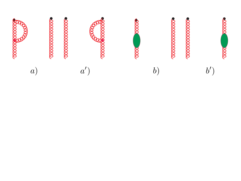
Figure 2: Self-energy-type diagrams

UV-divergent terms similar to those in Eq. (24) are also present in the gluon self-energy-type diagrams shown in Fig. 2. The diagrams $2a)$ and $2a^{\prime})$ together give

$$F_{(2a+2a^{\prime})}(x,q,\epsilon_{1},\epsilon_{2})= -\delta(1-x)\frac{\alpha_{s}}{\pi}C_{A}\frac{3}{4}\left(\frac{1}{\epsilon_{\mathrm{UV}}}-\frac{1}{\epsilon_{\mathrm{IR}}}+\ln\frac{\mu_{\mathrm{UV}}^{2}}{\mu_{\mathrm{IR}}^{2}}\right)\Pi(q,\epsilon_{1},\epsilon_{2})$$

$$+\{x\to-x\}\ .$$ (26)

The gluon self-energy diagrams $2b),2b^{\prime})$ give

$$F_{(2b+2b^{\prime})}(x,q,\epsilon_{1},\epsilon_{2}) =\delta(1-x)\frac{\alpha_{s}}{\pi}\left(\frac{5}{12}C_{A}-\frac{1}{3}T_{F}n_{f}\right)\left(\frac{1}{\epsilon_{\mathrm{UV}}}-\frac{1}{\epsilon_{\mathrm{IR}}}+\ln\frac{\mu_{\mathrm{UV}}^{2}}{\mu_{\mathrm{IR}}^{2}}\right)\Pi(q,\epsilon_{1},\epsilon_{2})$$

$$+\{x\to-x\}\ .$$ (27)

Combining Eqs. (24), (26) and (27) we obtain

$$\frac{\alpha_{s}}{2\pi}\frac{5}{2}C_{A}-\frac{\alpha_{s}}{\pi}\frac{3}{4}C_{A}+\frac{\alpha_{s}}{\pi}\left(\frac{5}{12}C_{A}-\frac{1}{3}T_{F}n_{f}\right)=\frac{\alpha_{s}}{4\pi}\left(\frac{11}{3}C_{A}-\frac{4}{3}T_{F}n_{f}\right)=\frac{\alpha_{s}}{4\pi}\beta_{0}$$ (28)

as the coefficient accompanying $\left({1}/{\epsilon_{\mathrm{UV}}}-{1}/{\epsilon_{\mathrm{IR}}}+\ln({\mu_{\mathrm{UV}}^{2}}/{\mu_{\mathrm{IR}}^{2}})\right)$. This result is in agreement with the fact that the combination $G^{2}\beta(\alpha_{s})/\alpha_{s}$ is related to the trace anomaly Chanowitz:1972vd ; Crewther:1972kn ; Collins:1976yq , and $g^{2}G_{\mu\nu}(0)G^{\mu\nu}(0)$ does not depend on the UV scale $\mu_{\rm UV}$ at one loop Kluberg-Stern:1975ebk ; Nielsen:1977sy . Hence, the anomalous dimension of $G^{2}$ at one loop should be opposite to that of $g^{2}$, i.e., proportional to $\beta_{0}$ (see, e.g., Ref. Tarrach:1981bi ).

The “Sudakov” term of Eq. (25) is UV finite. It does not contain the UV parameter $\mu_{\mathrm{UV}}$, and thus it does not affect the relation between the functions $F_{1}^{(1)}(x,q^{2},\mu_{\mathrm{UV}}^{2})$ at different evolution scales $\mu_{\mathrm{UV}}$, which we will denote simply as $\mu_{i}$. Namely, for $x\geq 0$ we have

$$F_{1}^{(1)}(x,q^{2},\mu_{1}^{2})= F_{1}^{(1)}(x,q^{2},\mu_{2}^{2})+\frac{\alpha_{s}}{\pi}\,\left\{C_{A}\bigg{[}\frac{\theta(0\leq x\leq 1)}{1-x}\bigg{]}_{+}+\frac{\beta_{0}}{4}\delta(1-x)\right\}\ln\frac{\mu_{1}^{2}}{\mu_{2}^{2}}$$ (29)

and similarly for $x\leq 0$. As indicated earlier, the $F_{2}^{(1)}\left(x,q^{2}\right)$ function contains a “zero mode” $\delta(x)$ term

$$F_{2}^{(1)}\left(x,q^{2}\right)= \frac{\alpha_{s}}{\pi}C_{A}q^{2}\left[(1-x)\theta(0\leq x\leq 1)-\frac{1}{2}\delta(x)\right]+\{x\to-x\}\ .$$ (30)

However, the function $F_{2}^{(1)}\left(x,q^{2}\right)$ disappears in the $q^{2}\to 0$ limit, and does not contribute to the “forward” PDF $F(x)$.

Recall that so far “$x$” had the meaning of the fraction of initial momentum $p$. So, if the initial momentum is $yp$, then the active gluon momentum is $xyp$. The usual convention is to use $xp$ for the active gluon momentum and $(x/z)p$ for the initial momentum. The ratio of the active gluon momentum to the initial one is then given by $z$. This allows us to use the kernel given by Eq. (29) (changing there $x$ into $z$) to write the evolution equation for the “forward” PDF $F(x,\mu^{2})$. Since $F(x,\mu^{2})=F(-x,\mu^{2})$, it is sufficient to write the equation for $x\geq 0$:

$$F(x,\mu_{1}^{2})= F(x,\mu_{2}^{2})+\frac{\alpha_{s}}{2\pi}\,\ln\left(\frac{\mu_{1}^{2}}{\mu_{2}^{2}}\right)\,\int_{x}^{1}\frac{dz}{z}P_{gg}^{F}(z)\,F(x/z,\mu_{2}^{2})\ ,$$ (31)

where

$$P_{gg}^{F}(z)=\frac{\beta_{0}}{2}\delta(1-z)+C_{A}\bigg{[}\frac{2}{1-z}\bigg{]}_{+}\$$ (32)

is the $gg$-component of the 1-loop evolution kernel for the “gluon condensate” PDF $F(x,\mu^{2})$. The lower limit of integration over $z$ in Eq. (31) reflects the fact that $F(y,\mu^{2})$ vanishes for $y>1$.

8 Summary and conclusions

In this paper, we have presented the results for one-loop corrections to the “gluon condensate” PDF $F(x)$ introduced in Ref. Hatta:2020iin . In the same paper it was suggested that this twist-4 distribution may have “zero mode” $\delta(x)$ terms. Such terms, in fact, have been observed in one-loop diagrams for quark twist-3 PDFs Burkardt:2001iy ; Aslan:2018tff .

According to our results, the $\delta(x)$ terms are absent in the one-loop expressions for the twist-4 gluon PDF $F(x)$. Still, we found the $\delta(x)$ term in the one-loop correction to the $\xi=0$ GPD $F(x,q^{2})$, where $q$ is the momentum transfer between the initial and the final gluons. This term is accompanied by the $q^{2}$ factor, and disappears in the forward $q=0$ limit. Another observation is that the spin structure of this “zero mode” term is different from that of the tree-level contribution. Using the Schwinger parametric representation in our studies of the “zero mode” terms, we have presented a simple way of analyzing the origin of the $\delta(x)$ terms in the Feynman diagram contributions.

Our calculations also shed light on the perturbative evolution properties of the twist-4 “gluon condensate” PDF $F(x)$. In particular, the final result of our paper provides explicit expression for the previously unknown $gg$-component of its evolution kernel .

Setting the framework for our calculations, we have proposed to switch to nonforward kinematics. Using this approach, we were able to get a nonzero result for the tree-level matrix element in a situation when the external gluons are on-shell.

Our study has clearly demonstrated the crucial role of strict compliance with the gauge invariance requirements. Using on-shell external gluons, we have obtained the same result both in Feynman and light-cone gauges. This outcome may be contrasted with the calculations involving off-shell external gluons, that have resulted in two different expressions in these two gauges. Attracting attention to this issue, we repeat that our results do not agree with those of the original attempt Hatta:2020iin of one-loop calculations of $F(x)$ for the gluon target. The reason for the discrepancy is the use of virtual external gluons in Ref. Hatta:2020iin .

These observations create an alarming warning for ongoing projects (see, e.g., Ref. Wang:2019tgg ) to renormalize gluon operators on the lattice with the help of matrix elements calculated for highly virtual gluon states.

References

- (1) R. P. Feynman, Photon-hadron interactions. Reading, 1972.
- (2) X. Ji, Fundamental Properties of the Proton in Light-Front Zero Modes, Nucl. Phys. B (2020) 115181, [2003.04478].
- (3) Y. Hatta and Y. Zhao, Parton distribution function for the gluon condensate, Phys. Rev. D 102 (2020) 034004, [2006.02798].
- (4) M. Burkardt and Y. Koike, Violation of sum rules for twist three parton distributions in QCD, Nucl. Phys. B 632 (2002) 311–329, [hep-ph/0111343].
- (5) G. Leibbrandt, Introduction to Noncovariant Gauges, Rev. Mod. Phys. 59 (1987) 1067.
- (6) F. Aslan and M. Burkardt, Singularities in Twist-3 Quark Distributions, Phys. Rev. D 101 (2020) 016010, [1811.00938].
- (7) Y. Hatta, -odd gluonic operators in QCD spin physics, Phys. Rev. D 102 (2020) 094004, [2009.03657].
- (8) A. V. Radyushkin, On Spectral Properties of Parton Correlation Functions and Multiparton Wave Functions, Phys. Lett. B 131 (1983) 179–182.
- (9) A. V. Radyushkin, Quark pseudodistributions at short distances, Phys. Lett. B 781 (2018) 433–442, [1710.08813].
- (10) I. Balitsky, W. Morris and A. Radyushkin, Gluon Pseudo-Distributions at Short Distances: Forward Case, Phys. Lett. B 808 (2020) 135621, [1910.13963].
- (11) S. Zhao, in preparation, .
- (12) Y.-S. Liu, W. Wang, J. Xu, Q.-A. Zhang, J.-H. Zhang, S. Zhao et al., Matching generalized parton quasidistributions in the RI/MOM scheme, Phys. Rev. D 100 (2019) 034006, [1902.00307].
- (13) X. Ji, A. Schäfer, X. Xiong and J.-H. Zhang, One-Loop Matching for Generalized Parton Distributions, Phys. Rev. D 92 (2015) 014039, [1506.00248].
- (14) S. Bhattacharya, K. Cichy, M. Constantinou, A. Metz, A. Scapellato and F. Steffens, The role of zero-mode contributions in the matching for the twist-3 PDFs and , Phys. Rev. D 102 (2020) 114025, [2006.12347].
- (15) M. S. Chanowitz and J. R. Ellis, Canonical Anomalies and Broken Scale Invariance, Phys. Lett. B 40 (1972) 397–400.
- (16) R. J. Crewther, Nonperturbative evaluation of the anomalies in low-energy theorems, Phys. Rev. Lett. 28 (1972) 1421.
- (17) J. C. Collins, A. Duncan and S. D. Joglekar, Trace and Dilatation Anomalies in Gauge Theories, Phys. Rev. D 16 (1977) 438–449.
- (18) H. Kluberg-Stern and J. B. Zuber, Renormalization of Nonabelian Gauge Theories in a Background Field Gauge. 2. Gauge Invariant Operators, Phys. Rev. D 12 (1975) 3159–3180.
- (19) N. K. Nielsen, The Energy Momentum Tensor in a Nonabelian Quark Gluon Theory, Nucl. Phys. B 120 (1977) 212–220.
- (20) R. Tarrach, The renormalization of FF, Nucl. Phys. B 196 (1982) 45–61.
- (21) W. Wang, J.-H. Zhang, S. Zhao and R. Zhu, Complete matching for quasidistribution functions in large momentum effective theory, Phys. Rev. D 100 (2019) 074509, [1904.00978].