Algorithms for Interference Minimization in Future Wireless Network Decomposition

Abstract

We propose a simple and fast method for providing a high quality solution for the sum-interference minimization problem. As future networks are deployed in high density urban areas, improved clustering methods are needed to provide low interference network connectivity. The proposed algorithm applies straightforward similarity based clustering and optionally stable matchings to outperform state of the art algorithms. The running times of our algorithms are dominated by one matrix multiplication.

I Introduction

One of the typical problems in algorithmic graph theory is to assign the vertices of a graph to partition clusters under some optimization condition. These general problem formulations have ample applications in everyday life. One of the very first applications of this kind was discussed by [1] in KL70 ([1]): let $G$ be an edge weighted graph (the weights are real numbers). The goal is to partition the graph into classes of at most $k$ vertices with minimum weighted edge cut. The graph itself represents a complicated electronic design to be placed on printed circuit cards, where each card can contain at most $k$ components and where the electronic connections among the cards are expensive. They observed that there is very small chance to solve the problem exactly. (The notion of NP-hardness was still at least one year away.) Therefore they suggested a heuristic: let’s start with a feasible configuration, then improve the design by exchanging vertices between the partition classes.

From that time on different graph partition problems are abundant in applied graph theory. While the continuous clustering problems (for example, vertices on surfaces or in higher dimensional spaces) can be often solved almost exactly (for example, with the Lagrange multiplier method or the spectral clustering methods, etc., see [2]), the graph partition problems usually need sophisticated heuristics. In [3] the authors surveyed a number of useful weight functions for the graph partitioning problem, and studied extensions of vector based clustering methods to graph partitioning problems.

Such graph partitioning problems arise naturally for large scale wireless networks. Large scale cellular networks have been designed, from the beginning, based on the idea of network decomposition [4]. Dividing a large area into a number of cells where a base station (BS) is placed at the center of each cell and serves users who fall into its coverage. In this way the original large-scale network is decomposed into multiple subnetworks which operate independently. This idea is simple, but design is infected by the well-known cell-edge problem [5]: users located at the cell edge area would suffer from strong interference from the neighboring BSs.

With coordinated multipoint (CoMP) transmission from multiple BSs, the network is decomposed into clusters of cells, where BSs in the same cluster would jointly serve the users. Therefore the typical approach was to cluster the BSs, then distribute the users among the defined clusters. With a fixed and a-priori (the signal-strength of the users are unknown) BS clustering pattern, nevertheless, users at the cluster edge still suffer from strong interference from neighboring clusters.

In this paper we provide a simple and fast method for constructing clustering of wireless networks with low sum-interference [3] that are applicable for real-time clustering in future wireless networks. Our proposed algorithms are significantly different from previous approaches and typically outperform those.

I-A Related Work

[6] introduced a new network model ([6]) for optimizing the clustering process, where the BSs and the users are clustered in parallel to minimize the sum-interference. [6] apply a widely used eigenvector based method called spectral clustering to construct the clusters. Spectral clustering solves a relaxed quadratic programming problem and constructs the clusters by discretizing the continuous solution. This method more-or-less represents the state of the art, so we will evaluate our methods in comparison to it.

II Interference Minimization Problem

II-A Problem Description

Let $\mathcal{G}=(V,\mathcal{E})$ be the complete bipartite graph, with a non-negative real weight function $w:\mathcal{E}\rightarrow\mathbb{R}^{\geq 0}$ on the edges. One class, $U$, denotes the users and the other class, $B$, denotes the set of all base stations (BSs). (So $V=U\cup B$.) The weight function denotes the interference between a BS and a user, in the case if they are in different clusters under the proposed vertex partition. (In the bipartite graph of course there is no edges among users, and among BSs.) Our goal is to minimize the total interference (described later on) under the defined clustering. This description does not ensure the condition that each user is served by some BSs. Therefore we add the extrinsic condition, that there is no cluster which contains only users, but no BSs. (Clusters with only BSs are allowed. The BSs in such clusters will be turned off temporarily.)

For a vertex subset $S$ in the graph $G$ let $w(S)$ denote

$$w(S):=\sum_{i,j\in S}w_{i,j}\quad\text{and}\quad\bar{w}(S):=\sum_{i\in S,j\not\in S}w_{i,j}.$$ (1)

For a fixed the number $M\in\mathbb{N}$, take a partition $\mathcal{C}$ of $V$ with $M$ clusters: $\mathcal{C}=\{C_{1},\ldots,C_{M}\}$. Consider the following optimization problem:

Problem 1 (Interference minimization (IM) problem with fixed $M$).

$$\min_{\mathcal{C}\in\Pi_{M}(\mathcal{G})}\sum_{m=1}^{M}\frac{\bar{w}(C_{m})}{w(C_{m})}.$$ (2)

The objective function is not the sum of the cut numbers but a normalized one. The reason for this is that the purely cut number based optimization will provide often very unbalanced partition class sizes. This is described in detail in [6], after equation (3) of that paper.

There is a technical problem hidden in eq. 2: by the formulation of the denominator, it can occur that a cluster contains zero BS or zero users. In both cases the denominator is zero. If there is a cluster without BSs, then the users of this cluster are not associated to any BS and the interference metric is infinite (or undefined). When a cluster contains at least one BS and zero users, then we can imagine that the stations will be switched off temporarily, that is, they are not considered as a source of interference.

To be able to use our procedure in practical application (like on-line optimization of users’ distribution among base stations in 5G mobile networks) we have some further considerations. Our secondary objectives are the follows:

• Phase 1: We want a fast, centralized algorithm to find an initial solution.

• Phase 2: During the calls the users may move away from the BSs of a given cluster, some may finish the calls, while others (currently not represented in the bipartite graph) may initiate calls. Therefore we need an incremental algorithm, that is able adaptively change the edge weights and/or can update the actual vertices. This phase must be initiated and managed distributively by the users.

• In every few seconds Phase 1 should be executed again (centrally) to find a new optimal clustering solution.

In practical applications the clusters cannot be arbitrarily complex (from an engineering point of view), therefore we consider an upper bound $T$ on the possible numbers of the BSs in any cluster. This component is a new addition to the model, it was not considered earlier. In previous work, the engineering complexity of the BSs’ clusters was handled indirectly. One possible way to do so was suggested by [6] in [6].

At first they proved that the minimum value in (2) is monotone increasing as the value $M$ is increasing.

Theorem 1 ([6], Theorem 1 in [6]).

$$\min_{\mathcal{C}\in\Pi_{M}(\mathcal{G})}\sum_{m=1}^{M}\frac{\bar{w}(C_{m})}{w(C_{m})}\leq\min_{\mathcal{C}\in\Pi_{M+1}(\mathcal{G})}\sum_{m=1}^{M+1}\frac{\bar{w}(C_{m})}{w(C_{m})}.$$ (3)

Then they introduced the Max-Num problem: here they want to increase the number $M$ as long as the minimum value in (2) is still smaller than a relative small, given positive number. [6] proposed a new approach to solve this latter problem. At first they reformulated the question, using matrix computation, to describe the constrains. This reformulation of the Max-Num problem is NP-hard, due to the discretization. Then this was relaxed to continuous constrains. Next a good heuristic was developed for the problem, using a generalized spectral clustering method. Unfortunately, the computational complexity of the method is still quite high for fast, practical application. Furthermore the indirect approach does not ensure always that the provided clusters are “simple” enough.

In the remaining part of this paper we propose a new heuristic to solve Problem 1 directly to overstep the previous weaknesses.

III Dot-Product Hierarchical Clustering for IM

In this section we describe a new and simple heuristic for the IM problem. We cluster BSs based on a new similarity measure. The novelty lies in the fact that the clustering is made on the basis of a relation between BSs which is derived from the relation among BSs and users. At first we discuss the original problem formulation: the value $M$ is an input parameter. We will come back later to the variation of the problem where an upper bound is given on the maximum size of BS clusters.

III-A Similarity Measure

A cursory study of eq. 2 says that we want to decompose the graph in such a way that each cluster contains high weight edges, while the cuts among the clusters consist of low weight edges. Let’s assume that the weight function is given via the matrix $w$ where the rows correspond to the BSs, and the columns correspond to the users. Then each $w_{i,j}$ is the weight between BS $i$ and user $j$.

Let $w_{i,\bullet}$ denote the row of BS $i$, and let $w_{\bullet,j}$ denote the column of user $j$. So $w={[w_{i,\bullet}]}_{i\in B}={[w_{\bullet,j}]}_{j\in U}$. Our heuristics would say that the larger the number of high weighted common neighbors of two BSs, the more advantageous it is for the two BSs to be included in the same cluster. So define the similarity function

$$\rho:B\times B\rightarrow\mathbb{R}^{\geq 0}\quad\text{with}\quad\rho(i,j):=\frac{w_{i,\bullet}^{T}\cdot w_{j,\bullet}}{\|w_{i,\bullet}\|\cdot\|w_{j,\bullet}\|}$$ (4)

among the BSs, where $\|\cdot\|$ is the Euclidean-norm. The enumerator of eq. 4 is what we refer to by dot product. The similarity $\rho$ depends only on the weights between the users and the BSs. Clearly, the bigger the product, the greater the similarity between the BSs.

In the interference minimization model, a set of BSs in a cluster behave as one BS. Indeed, if $\{C_{1},\ldots,C_{M}\}\in\Pi_{M}(\mathcal{G})$ minimizes eq. 2, then replacing the set of BSs in cluster $C_{i}$ with just one new BS $b_{\text{new}}$ whose weight to user $j$ is $\sum_{k\in C_{i}\cap B}w_{k,j}$ preserves the optimum, and the interference metric takes this optimum on $\left\{C_{1},\ldots,C_{i-1},C_{i}-B+\{b_{\text{new}}\},C_{i+1},\ldots,C_{M}\right\}$. Define

$$\mathrm{vec}(B_{k})=\sum_{i\in B_{k}}w_{i,\bullet}$$ (5)

as the sum of the signal strength vectors of the BSs in $B_{k}$. The similarity function $\rho$ can be naturally extended to sets of BSs:

$$\begin{split}&\rho:2^{B}\times 2^{B}\rightarrow\mathbb{R}^{\geq 0}\quad\text{with}\\ &\rho(B_{k},B_{m}):=\frac{{\mathrm{vec}(B_{k})}^{T}\cdot\mathrm{vec}(B_{m})}{\|\mathrm{vec}(B_{k})\|\cdot\|\mathrm{vec}(B_{m})\|}.\end{split}$$ (6)

III-B Hierarchical Clustering: Defining BS Clusters

Next we describe our hierarchical clustering algorithm: we call it DPH-clustering, short for dot-product hierarchical clustering. Let the fixed integer $M$ be the desired number of clusters.

There seems to be no clear leading method to cluster $B$ based on $\rho$. Our choice is a simple hierarchical clustering method: merge two clusters that have the highest similarity $\rho$ between them until the desired number of clusters is reached. As we will soon see, this works reasonably well. Here we want to emphasize that using normalization in eqs. 4 and 6 is a natural idea.

Let the initial partition be $\mathcal{B}_{0}$ which contains a cluster for each BS in $B$ (thus $|B|=|\mathcal{B}_{0}|$). We merge two clusters in each of the $|B|-M$ rounds iteratively to obtain a sequence of partitions $\mathcal{B}_{0},\mathcal{B}_{1},\ldots,\mathcal{B}_{|B|-M}$ of $B$, where $|\mathcal{B}_{r}|=|B|-r$. $\mathcal{B}_{r}$ is obtained from $\mathcal{B}_{r-1}$ by merging the two clusters of $\mathcal{B}_{r}$ with the largest similarity $\rho$ between them as defined by eq. 6.

In Alg. 1 we will maintain $\rho(B_{k},B_{m})$ for every $B_{k},B_{M}\in\mathcal{B}_{r}$ as follows. Let us define the symmetric function $\mathit{dot}$ for every $k=1,\ldots,M$ as

$$\mathit{dot}(B_{k},B_{m})={\mathrm{vec}(B_{k})}^{T}\cdot\mathrm{vec}(B_{m}).$$ (7)

If $\mathit{dot}$ is already computed for every pair in $\mathcal{B}_{r}\times\mathcal{B}_{r}$, then $\rho$ can be computed via three scalar operations for any pair of clusters in $\mathcal{B}_{r}\times\mathcal{B}_{r}$, since

$$\rho(B_{k},B_{m})=\frac{\mathit{dot}(B_{k},B_{m})}{\sqrt{\mathit{dot}(B_{k},B_{k})\cdot\mathit{dot}(B_{m},B_{m})}}.$$ (8)

Algorithm 1 Hierarchical clustering based on the similarity function $\rho$

function DPH-clustering($B,w,M$)

     $\mathcal{B}_{0}\leftarrow\binom{B}{1}$

     $\mathit{dot}\leftarrow w\cdot w^{T}$ $\triangleright$ matrix multiplication

     for $r=0$ to $|B|-M-1$ do

         $\displaystyle\{B^{\prime},B^{\prime\prime}\}\leftarrow\operatorname*{arg\,max}_{\{B_{k},B_{m}\}\in\binom{\mathcal{B}_{r}}{2}}\rho(B_{k},B_{m})$$\triangleright$ (8)

         $\mathcal{B}_{r+1}=\mathcal{B}_{r}-\{B^{\prime},B^{\prime\prime}\}+\{B^{\prime}\cup B^{\prime\prime}\}$

         update $\mathit{dot}$ $\triangleright$ $\mathcal{O}(b)$ scalar operations

     end for

     return $\mathcal{B}_{|B|-M}$

end function

The running time of Alg. 1 is easily seen to be in $\mathcal{O}\left(b^{2}u+(b-M)\cdot b^{2}\right)$, because when two clusters are merged, $\mathit{dot}$ can be updated by summing the corresponding two rows and two columns. Moreover, we may store the $\rho$-values of pairs in $\mathcal{B}_{r}\times\mathcal{B}_{r}$ in a max-heap: when two clusters are merged, at most $2b$ values need to be removed and at most $b$ new values need to be inserted into the heap which contains the at most $\binom{b}{2}$ elements of the set $\{\rho(B_{k},B_{m})\ |\ \{B_{k},B_{m}\}\in\binom{\mathcal{B}_{r}}{2}\}$. With these optimizations, the for-loop takes at most $\mathcal{O}\left((b-M)\cdot b\log b\right)$ steps, thus the running-time of the algorithm is dominated by the matrix multiplication $w\cdot w^{T}$. There are many techniques to accelerate the multiplication of matrices, which we do not discuss here, but let us mention that if $b\simeq u$ then $w$ can be padded with zeros to a square matrix, whose multiplication can be tackled with recursive divide-and-conquer methods. We will discuss alternative strategies for the case when $b$ is much larger than $u$ in Section IV.

III-C Hierarchical Clustering: Assigning Users to BS Clusters

Let $\mathcal{B}_{|B|-M}=\{B_{1},\ldots,B_{M}\}$ be the final partition produced by the hierarchical clustering. The final output will be of the form $\mathcal{C}=\cup_{k=1}^{M}\{B_{i}\cup U_{i}\}$, so it only remains to find a clustering $\mathcal{U}=\{U_{1},\ldots,U_{M}\}$ of $U$. We assign each user $j\in U$ to the cluster $U_{\ell}$ where

$$\ell=\operatorname*{arg\,max}_{k\in[1,M]}\sum_{i\in B_{k}}w_{i,j}.$$ (9)

Algorithm 2 Dot-product hierarchical clustering on $B$ then assigning each element of $U$ to the best cluster. The algorithm is relatively efficient if $|U|$ is not much smaller than $|B|$.

function Similarity Clustering($B,U,w,M$)

     $B_{1},\ldots,B_{M}\leftarrow\textsc{DPH-clustering}(B,w,M)$

     $U_{1},\ldots,U_{M}\leftarrow$ empty clusters

     for all $j\in U$ do

         $\ell\leftarrow\operatorname*{arg\,max}_{k\in[1,M]}\sum_{i\in B_{k}}w_{i,j}$

         add $j$ to $U_{\ell}$

     end for

     return $\{B_{k}\cup U_{k}\ |\ U_{k}\neq\emptyset\}$

end function

The assignment defined by eq. 9 is easy to compute, and it is trivial to assign new users to a cluster. It may happen that a BS cluster is left without users: such clusters are discarded at cost of decreasing the number of clusters, thus the output clustering will not reach the target cardinality $M$.

Discarding clusters that only intersect one of the classes is not an issue if the hierarchical clustering is performed on $B$. However, were we to call $\textsc{DPH-clustering}(U,w^{T},M)$ to take advantage of computing a smaller matrix product, we might discard user-clusters without BSs. To avoid creating clusters without BSs, we supply alternative Phase 2 algorithms for assigning elements of the yet unclustered class to the clusters of the already DPH-clustered class in Section IV.

Since we had chosen the spectral clustering method as our baseline, next we analyse the differences between the two approaches: Alg. 2 has immediate advantages over the spectral clustering method:

1. Hierarchical clustering is much faster than the spectral clustering method: the running time is dominated by multiplying two matrices of size $b\cdot u$.

2. Using $\rho$ as the similarity function, the slight movements of the users change the similarity measure only slightly, therefore we may assume that the BS clustering is not necessarily updated in real time; a periodic (every couple hundred milliseconds) updating of $\mathcal{B}$ will be sufficient. This seems to be an adequate answer for the problem of Phase 2.

3. It is easy to modify the hierarchical clustering to respect an upper bound $T$ on the size of the BS clusters, see Section VI.

This concludes the description of our method in the case when there are fewer BSs than users. In practice we expect this to be the case. However, Alg. 2 does not perform efficiently in simulations (see Section V) if the number of BSs is far fewer than the number of users. We deal with this case in the following section.

IV When There Are More BSs Than Users

Suppose that $B$ has many more elements than $U$. We can switch the roles of $B$ and $U$, and perform the hierarchical clustering (Alg. 1) on $U$ instead of $B$. There is a large computational advantage over the original approach, since the running time is dominated by the complexity of the matrix multiplication of $w^{T}\cdot w$ vs. $w\cdot w^{T}$. However, the slight asymmetry in evaluating eq. 2 that we hinted at earlier becomes dangerous: given a clustering $\mathcal{U}=\{U_{1},\ldots,U_{M}\}$, if we assign each BS $i\in B$ to $B_{\ell}$ (i.e., cluster $C_{\ell}$) where

$$\ell=\operatorname*{arg\,max}_{k\in[1,M]}\sum_{j\in U_{k}}w_{i,j},$$ (10)

we may end up with $C_{k}=U_{k}$ for some $k$. Let us describe two possible solutions to avoid BS-less clusters.

IV-A Assigning a BS to User Clusters Via Maximum Cardinality Matchings

One way to overstep (not to solve) this problem is simply assigning a unique BS to each user-cluster. After that we can assign the remaining BSs in whatever manner we chose, for example, as described by eq. 10. Choosing these unique BS is not necessarily a trivial task, it is equivalent to finding a matching of $\mathcal{U}$ into $B$ where the edges have relatively large weights, preferably.

We try to find a maximum cardinality (and maximum weight) matching of $\mathcal{U}$ into $B$ such that if $i\in B$ is matched to $U_{k}$ then $w(U_{k}\cup\{i\})\neq 0$ (so that the interference cannot be infinite, no matter how we complete the clustering). Even if the complexity of the maximum cardinality matching is prohibitive in some of our applications, there exist approximate solutions that provide a log-linear complexity. Using the algorithm of [7] [7], the $(1-\varepsilon)$-approximate solution for the matching can be computed in $\mathcal{O}(bu\varepsilon^{-1}\log\varepsilon^{-1})$ time. Therefore the running time of Alg. 1 is also dominated by the matrix multiplication $w^{T}\cdot w$ in DPH-clustering.

Algorithm 1 Dot-product hierarchical clustering on $U$, then assigning one BS to each cluster of $U$, and assigning the remaining BSs to the best cluster. The algorithm is relatively efficient if $|B|$ is larger than $|U|$.

function DPH+matching+best($B,U,w,M$)

     $U_{1},\ldots,U_{M}\leftarrow\textsc{DPH-clustering}(U,w^{T},M)$

     $B_{1},\ldots,B_{M}\leftarrow$ empty clusters

     $E\leftarrow$ approx. max. card. max. weight matching $\{U_{1},\ldots,U_{M}\}$ into $B$ using positive weight edges, see [7]

     for all $i\in B$ do

         if $U_{\ell}$ is joined to $i$ in $E$ then

              add $i$ to $B_{\ell}$

         else

              $\ell\leftarrow\operatorname*{arg\,max}_{k\in[1,M]}\sum_{j\in U_{k}}w_{i,j}$

              add $i$ to $B_{\ell}$

         end if

     end for

     return $\{B_{k}\cup U_{k}\ |\ k=1,\ldots,M\}$

end function

IV-B Clustering $B$ via Stable Matchings

In this subsection we provide an alternative method based on the stable matching approach. A matching between two classes of entities is stable if there is no pair of entities that both prefer each other over their current match. The problem to find such a matching has many applications in economics, see the works of Roth and Shapley [8]. In a generalization of this problem entities in the first class can be matched to many entities of the second class; this version is colloquially known as the college admissions problem (many-to-one matching).

The stable matching algorithm of Gale and Shapley [9] can be used to overcome the base-station-less cluster problem. In our (many-to-one) stable matching setup, each cluster in $\mathcal{U}$ and each BS in $B$ is assigned a list of real numbers corresponding to the members of the other class. We are looking for a (many-to-one matching) which is stable with respect to the preference values: if $U_{1}b_{1}$ and $U_{2}b_{2}$ are in the stable matching, then we must have

$$\mathrm{pref}(b_{1};U_{1}) \geq\mathrm{pref}(b_{1};U_{2})\text{ or}$$

$$\mathrm{pref}(U_{2};b_{2}) \geq\mathrm{pref}(U_{2};b_{1}).$$

Let the preference of BS $i\in B$ for the user-cluster $U_{k}$ be

$${\mathrm{pref}}(i;U_{k})=\sum_{j\in U_{k}}w_{i,j},$$ (11)

that is, the first preference of a base-stations $i$ is the user cluster assigned by eq. 10. However, we define the preferences asymmetrically. Let the preference of cluster $U_{k}$ for BS $i\in B$ be

$${\mathrm{pref}}(U_{k};i)=-\frac{\sum_{j\in U}w_{i,j}}{\sum_{j\in U_{k}}w_{i,j}}.$$ (12)

Note the negative sign in eq. 12: the cluster prefers a small fraction in absolute value. The reasoning for these preference values will be explained shortly.

The stable matching algorithm can be used to find not just one matching, but a complete clustering of the not yet clustered class $B$ (stable marriage vs. college admissions). This is equivalent to finding a many-to-one matching of $B$ to $\mathcal{U}$. Given a clustering $\mathcal{U}=\{U_{1},\ldots,U_{M}\}$ of $U$ (constructed by, say, DPH-clustering), we set the capacity and usage of $B_{k}$ as follows:

$$\mathrm{capacity}(k) =\sum_{j\in U_{k}}\sum_{i\in B}w_{i,j},$$ (13)

$$\mathrm{usage}(k) =\sum_{i\in B_{k}}\sum_{j\in U}w_{i,j}.$$ (14)

A BS can be added (matched) to $B_{k}$ without extra maintenance steps as long as $\mathrm{usage}(k)\leq\mathrm{capacity}(k)$ holds even after the BS joins $B_{k}$. If $\mathrm{usage}(k)>\mathrm{capacity}(k)$ after a BS joins $B_{k}$, then remove the lowest-preference BS from $B_{k}$ if and only if $\mathrm{usage}(k)\geq\mathrm{capacity}(k)$ holds even after removal.

Definition 2 (Stable clustering).

A clustering $B_{1},\ldots,B_{M}$ of $B$ is stable if

• $\mathrm{usage}(k)-\sum_{j\in U}w_{\beta_{k},j}\geq\mathrm{capacity}(k)$ where $\beta_{k}=\operatorname*{arg\,min}_{\lambda\in B_{k}}\mathrm{pref}(U_{k};\lambda)$ for every $k=1,\ldots,M$, and

• for every $k\neq m$ and $\beta\in B_{k}$, $\gamma\in B_{m}$ we have $\mathrm{pref}(\beta;U_{k})\geq\mathrm{pref}(\beta;U_{m})$ or $\mathrm{pref}(U_{m};\gamma)\geq\mathrm{pref}(U_{m};\beta)$.

Algorithm 2 Extending a clustering $\mathcal{U}$ via stable matchings

function Stable clustering($B,U,w,M$)

     $U_{1},\ldots,U_{M}\leftarrow\textsc{DPH-clustering}(U,w^{T},M)$

     $B_{1},\ldots,B_{M}\leftarrow$ empty clusters

     while $\exists i\in B\setminus B_{1}\setminus\ldots\setminus B_{M}$ do

         let $U_{k}$ maximize $\mathrm{pref}(i;U_{k})$ among clusters which have not rejected $i$

         add $i$ to $B_{k}$

         let $\beta\leftarrow\operatorname*{arg\,min}_{\lambda\in B_{k}}\mathrm{pref}(U_{k};\lambda)$

         while $\mathrm{usage}(k)-\sum_{j\in U}w_{\beta,j}\geq\mathrm{capacity}(k)$ do

              remove $\beta$ from $B_{k}$, i.e., $U_{k}$ rejects $\beta$

              let $\beta\leftarrow\operatorname*{arg\,min}_{\lambda\in B_{k}}\mathrm{pref}(U_{k};\lambda)$

         end while

     end while

     return $\{B_{k}\cup U_{k}\ |\ k=1,\ldots,M\}$

end function

If $\mathrm{usage}(k)\geq\mathrm{capacity}(k)$ holds at some point during the execution of Alg. 2, then it holds at any later step too. Thus if a BS $\beta$ is rejected by each cluster, then the usage of every cluster increased above its capacity even without $\beta$’s contribution. This is a contradiction by the handshaking lemma, since $\sum_{k=1}^{M}\mathrm{capacity}(k)=\sum_{i\in B}\sum_{j\in U}w_{i,j}$. Therefore Alg. 2 terminates after at most $bu$ cycles of the outer while-loop, and when it terminates, every BS is associated to a cluster.

In other words, if $B_{1},\ldots,B_{M}$ is a clustering of $B$, then the sum of $\mathrm{usage}(k)$ is equal to the sum of $\mathrm{capacity}(k)$, which means that we can expect that there exists a small $\varepsilon>0$ such that for every $k$ we have $\mathrm{capacity}(k)\leq(1+\varepsilon)\cdot\mathrm{usage}(k)$. If that is so, then let $-c_{k}=\min_{i\in B_{k}}{\mathrm{pref}}(U_{k};i)$; we have

$$\frac{\bar{w}(C_{k})}{w(C_{k})} =\frac{\mathrm{capacity}(k)+\mathrm{usage}(k)}{w(C_{k})}-2\leq$$

$$\leq(2+\varepsilon)\frac{\mathrm{usage}(k)}{w(C_{k})}-2\leq(2+\varepsilon)c_{k}-2.$$

Note that we have equality if the BSs in $B_{k}$ are equally preferred by cluster $U_{k}$. In words, the higher the preferences of the associated BSs, the lower the sum-interference is, so eq. 12 is a reasonable choice, because we can more or less guarantee $\mathrm{capacity}(k)\simeq\mathrm{usage}(k)$ for each cluster $U_{k}$.

Observe, that the preferences can be extracted in $\mathcal{O}(Mb)$ time from the computations performed by the hierarchical clustering of $U$. By using binary heaps to represent the clusters $B_{1},\ldots,B_{M}$, we can insert and remove BSs in $\log b$ time. Since every BS tries to join each cluster at most once, the total running time is in $\mathcal{O}(Mb\log b)$. This is clearly dominated by the complexity of matrix multiplication in the hierarchical clustering algorithm.

V Experimentation

We have compared the performance of Similarity Clustering (Alg. 2), Stable Clustering (Alg. 2), and Spectral Clustering [6] in several scenarios. In each case, base-stations (BSs) and users are placed independently uniformly and randomly into $[0,1000]^{2}$ (a square with an area of $1\,\mathrm{km}^{2}$). The weight (or signal strength) between a BS and a user $b_{i},u_{j}\in[0,1000]^{2}$ is set to

$$w_{i,j}=\left\{\begin{array}[]{ll}{\|\mathrm{dist}_{\min}\|}^{-\alpha}&\text{ if }\|b_{i}-u_{j}\|\leq\mathrm{dist}_{\min},\\ {\|b_{i}-u_{j}\|}^{-\alpha}&\text{ if }\mathrm{dist}_{\min}\leq\|b_{i}-u_{j}\|\leq\mathrm{dist}_{\max},\\ 0&\text{ if }\mathrm{dist}_{\max}<\|b_{i}-u_{j}\|,\end{array}\right.$$

where we set the path loss component $\alpha=4$ (see [6, 4]), $\mathrm{dist}_{\min}=1$, and $\mathrm{dist}_{\max}=200$.

For the unconstrained 1 simulations show short running times and very low interference measures on the acquired clusterings compared to the spectral clustering method (at least when the number of users is larger than the number of BSs). While the paper [6] suggests that we should expect a small number of giant clusters, this is clearly not the case in our test runs. This phenomenon requires much better understanding.

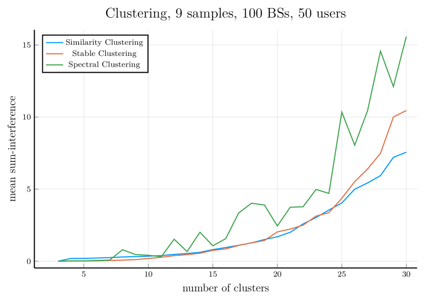
(a) For $M\leq 17$, Stable Clustering is consistently better than Similarity Clustering, which we suspect is another advantage of performing the DPH-clustering on the users’ side

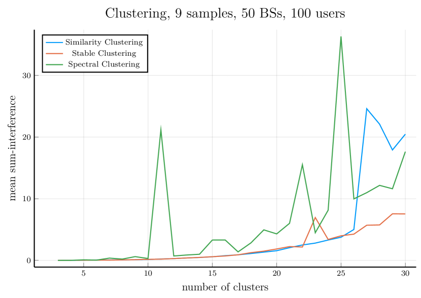
(b) For $M\geq 27$ clusters, Alg. 2 produces some clusters with very weak BS coverage

(c) The performance of both of our algorithms scale much more evenly than the performance of the output of Spectral Clustering

Figure 1: Mean sum-interference values as a function the number of clusters $M$

(a) Similarity Clustering, Alg. 2

(b) Stable Clustering, Alg. 2

(c) Spectral Clustering, see [6]

Figure 2: Comparison of the output of three clustering algorithms on 100 BSs and 50 users, $M=10$. Triangles and circles represent BSs and users, respectively

(a) Similarity Clustering, Alg. 2

(b) Stable Clustering, Alg. 2

(c) Spectral Clustering, see [6]

Figure 3: Comparison of the output of three clustering algorithms on 50 BSs and 100 users, $M=10$. Triangles and circles represent BSs and users, respectively

Fig. 1 compares the performance of the three mentioned algorithms in three different settings: when there are many more BSs than users and vica versa, and when there number of BSs is equal to the number of users. The plots correspond to the mean sum-interference values of the solutions provided by the algorithms over 9 random samples of BSs-user placements. In all three cases we find that our algorithms perform more consistently than the spectral clustering method, and the performance of Alg. 2 and Alg. 2 are similar when the number of clusters are not too large or the number of BSs is not much larger than the number of users.

Fig. 2 (50 BSs and 100 users) and Fig. 3 (100 BSs and 50 users) show example clusterings on the same BS-user placements each, respectively.

VI Conclusion and Further Considerations

This paper proposed a similarity based hierarchical clustering method for simple-and-fast wireless network decomposition in future wireless networks, with the goal of minimizing sum interference in the overall network. Moreover, stable matching were utilized to match BSs and users. Compared with state-of-the-art spectrum clustering method, simulation results demonstrated that our proposed algorithm could achieve better performance with much less complexity. Further considerations are listed below, which lead to future research directions.

• Suppose that the final clustering $\mathcal{B}$ on $B$ is restricted to clusters of size at most $T$. Running the DPH-clustering algorithm on $B$, we reject merging clusters whose total size is larger than $T$, i.e., we restrict our search for the largest similarity to pairs whose union has cardinality at most $T$. This allows one to control the maximum engineering complexity that arises in any cluster. The main issue with similarity clustering in this setting is that we run into discretization problems if $T$ is relatively small.

• It is also relatively easy to meaningfully modify Alg. 2, to say, not assign a BS to a lower preference than half of their maximum. For example, we may specify that if $i\in B_{k}$ in the final clustering then

  $$\mathrm{pref}(i,U_{k})\geq\frac{1}{2}\max_{\lambda\in\{1,\ldots,M\}}\mathrm{pref}(i,U_{\lambda}).$$

  If $i$ is rejected even by the least favored admissible cluster, then $i$ does not try to join clusters later on its preference list. Instead, when the Gale-Shapley algorithm completes, $i$ joins its most preferred cluster.

• Our proposed algorithms cluster every BS, even if using a BS in any cluster is causes more interference than not using it at all. This problem can be dealt with a trivial post-processing procedure: after the clusters $C_{1},\ldots,C_{M}$ are determined, delete a tower $i$ from $C_{k}$ if doing so decreases $\overline{w}(C_{k})/w(C_{k})$.

References

- [1] B. W. Kernighan and S. Lin “An efficient heuristic procedure for partitioning graphs” In The Bell System Technical Journal 49.2, 1970, pp. 291–307 DOI: 10.1002/j.1538-7305.1970.tb01770.x
- [2] Inderjit S. Dhillon, Yuqiang Guan and Brian Kulis “Kernel k-means: spectral clustering and normalized cuts” In Proceedings of the tenth ACM SIGKDD international conference on Knowledge discovery and data mining, KDD ’04 New York, NY, USA: Association for Computing Machinery, 2004, pp. 551–556 DOI: 10.1145/1014052.1014118
- [3] Inderjit S. Dhillon, Yuqiang Guan and Brian Kulis “Weighted Graph Cuts without Eigenvectors A Multilevel Approach” In IEEE Transactions on Pattern Analysis and Machine Intelligence 29.11, 2007, pp. 1944–1957 DOI: 10.1109/TPAMI.2007.1115
- [4] David Tse and Pramod Viswanath “Fundamentals of Wireless Communication” Cambridge University Press, 2005
- [5] David Gesbert et al. “Multi-Cell MIMO Cooperative Networks: A New Look at Interference” In IEEE Journal on Selected Areas in Communications 28.9, 2010, pp. 1380–1408 DOI: 10.1109/JSAC.2010.101202
- [6] Lin Dai and Bo Bai “Optimal Decomposition for Large-Scale Infrastructure-Based Wireless Networks” In IEEE Transactions on Wireless Communications 16.8, 2017, pp. 4956–4969 DOI: 10.1109/TWC.2017.2704095
- [7] Ran Duan and Seth Pettie “Linear-Time Approximation for Maximum Weight Matching” In Journal of the ACM 61.1, 2014, pp. 1:1–1:23 DOI: 10.1145/2529989
- [8] “The Sveriges Riksbank Prize in Economic Sciences in Memory of Alfred Nobel 2012” URL: https://www.nobelprize.org/prizes/economic-sciences/2012/summary/
- [9] D. Gale and L. S. Shapley “College Admissions and the Stability of Marriage” In The American Mathematical Monthly 69.1, 1962, pp. 9–15 DOI: 10.1080/00029890.1962.11989827